


1. Introduction
Convection is a dynamical process that governs heat transport and mixing in a variety of systems ranging from planetary and astrophysical flows to industrial devices. In that respect, a crucial question is how the heat flux in the system is connected with the temperature gradient. Near equilibrium, where both quantities are small, Fourier laws apply, and the heat flux is simply proportional to the temperature gradient. For larger values, the system enters a nonlinear then turbulent regime, where thermal energy is converted into mechanical energy, and the relation becomes nonlinear. The deviations from linearity are quantified by the relation between the Nusselt number  $Nu$, the ratio between the heat flux and its laminar value, and the Rayleigh number $Ra$, the non-dimensional temperature gradient.
In fluid mechanics, the paradigmatic system describing convection is a fluid enclosed in a volume, in which thermal energy is injected at the bottom via imposed heat flux or temperature gradient. Its dynamics is described by the Rayleigh–Bénard (RB) equations. Despite decades of theoretical, experimental and numerical developments, the scaling of the heat transfer in RB convection remains a subject of discussion and active research. In bounded domains at low  $Ra$, a simple argument by Malkus & Chandrasekhar (Reference Malkus and Chandrasekhar1954) based on the criticality of the thermal boundary layer gives $Nu\sim Ra ^{1/3}$, observed in many experiments (see Ahlers, Grossmann & Lohse (Reference Ahlers, Grossmann and Lohse2009) for a review). As we increase $Ra\to \infty$, viscous processes (and their associated boundary layers) are believed to become irrelevant, resulting in an ‘ultimate regime of convection’, where $Nu\sim Ra ^{1/2}$ (hereafter called ‘asymptotic ultimate regime’) (Spiegel Reference Spiegel1963; Grossmann & Lohse Reference Grossmann and Lohse2000), with possible logarithmic corrections (Kraichnan Reference Kraichnan1962; Grossmann & Lohse Reference Grossmann and Lohse2011) (hereafter called ‘ultimate regime’). Experimental or numerical observations of the (asymptotic) ultimate regime prove to be very difficult, and no final consensus has been reached so far about its existence in a pure RB setting (Doering & Constantin Reference Doering and Constantin1996; Chavanne et al. Reference Chavanne, Chillà, Castaing, Hébral, Chabaud and Chaussy1997; Zhu et al. Reference Zhu, Mathai, Stevens, Verzicco and Lohse2018, Reference Zhu, Mathai, Stevens, Verzicco and Lohse2019a; Urban et al. Reference Urban, Hanzelka, Králík, Macek, Musilová and Skrbek2019; Roche Reference Roche2020) (see Ahlers et al. (Reference Ahlers, Grossmann and Lohse2009) for a less recent but more synthetic review). When the gravity is artificially increased using centrifugal force, one can indeed observe hints of an ultimate regime (Jiang et al. Reference Jiang, Wang, Liu and Sun2022). On the other hand, various modifications of the RB geometry aiming at modifying the influence of the boundary layers result in experimental observation of a regime where $Nu\sim Ra ^{1/2}$: using highly elongated cells (Pawar & Arakeri Reference Pawar and Arakeri2016; Castaing et al. Reference Castaing, Rusaouen, Salort and Chilla2017), using rough (Ciliberto & Laroche Reference Ciliberto and Laroche1999; Rusaouën et al. Reference Rusaouën, Liot, Castaing, Salort and Chilla2018; Zhu et al. Reference Zhu, Stevens, Shishkina, Verzicco and Lohse2019b; Kawano et al. Reference Kawano, Motoki, Shimizu and Kawahara2021) or porous (Zou & Yang Reference Zou and Yang2021; Motoki, Kawahara & Shimizu Reference Motoki, Kawahara and Shimizu2022) boundaries, or radiatively heating the flow (Lepot, Aumaître & Gallet Reference Lepot, Aumaître and Gallet2018; Bouillaut et al. Reference Bouillaut, Lepot, Aumaître and Gallet2019).
From a numerical point of view, a simple way to remove boundary layers is to consider a triply periodic geometry, and heat the flow via an applied temperature gradient. This setting was first explored by Borue & Orszag (Reference Borue and Orszag1997), Lohse & Toschi (Reference Lohse and Toschi2003), Calzavarini et al. (Reference Calzavarini, Lohse, Toschi and Tripiccione2005) and Calzavarini, Lohse & Toschi (Reference Calzavarini, Lohse and Toschi2007) and called homogeneous RB (HRB) convection. The corresponding scalings and predictions are summarized in table 1. Although the results of those simulations are consistent with the predictions of Grossmann & Lohse (Reference Grossmann and Lohse2000) (hereafter called GL theory), they are undermined by several drawbacks: statistics polluted by the growth of uncontrolled exponential instabilities (Calzavarini et al. Reference Calzavarini, Doering, Gibbon, Lohse, Tanabe and Toschi2006) of unclear physical relevance, a small  $Ra$ and $\Pr$ range, sparse data points due to difficulties in running numerically challenging simulations. Indeed, pushing the Rayleigh number to large values increases the numerical burden beyond the capacity of present computers, as the number of grid points needed to describe the flow usually scales like $Re^{3}$ with $Re\sim Ra ^{1/2}$. In an attempt to reduce the number of degrees of freedom, models based on sparse interacting Fourier modes have been recently devised (Campolina & Mailybaev Reference Campolina and Mailybaev2018, Reference Campolina and Mailybaev2021). Those modes are evenly spaced points in logarithmic space (thus hereafter called log-lattice) and are interacting via nonlinear equations that are derived from the fluid equations by substituting for the convolution product a new operator that can be seen as a convolution on the log-lattice, and preserves all the main symmetries and conservation laws of the original equations. As such, log-lattices are likely to preserve properties of the original equations that are directly linked to these symmetries and conservation laws. This was indeed checked for the Burgers and Navier–Stokes equations in Fourier space (energy spectrum, energy transfers), over an unprecedented wide range of scales (Campolina & Mailybaev Reference Campolina and Mailybaev2021). Another interesting feature of log-lattices is that in one dimension, they encompass classical shell models of turbulence for special values of the log-lattice spacing (Campolina & Mailybaev Reference Campolina and Mailybaev2021), such as the Sabra shell model of turbulence (Gloaguen et al. Reference Gloaguen, Léorat, Pouquet and Grappin1985; Biferale Reference Biferale2003).
Table 1. Scaling predictions for HRB observables in the turbulent regime with and without friction. The observables are given in table 2. Here DNS stands for direct numerical simulation using regular Fourier modes (Calzavarini et al. Reference Calzavarini, Lohse, Toschi and Tripiccione2005) while LL refers to simulations using Fourier modes on a log-lattice (this paper). Parameters  $U_{ls}^2$ and $\varTheta _{ls}^2$ are large-scale kinetic and thermal energy. Exponents are computed by fitting over $Ra>10^{7}$ (respectively $1<\Pr <50$) for varying $Ra$ (respectively $\Pr$). Errors represent standard deviation of fit parameters.

One-dimensional (1-D) shell models of turbulence were used previously in the context of HRB (Ching & Ko Reference Ching and Ko2008) in an effort to increase the  $Ra$ and $\Pr$ range of results. They successfully display the asymptotic ultimate regime of convection, at the price of tuning several parameters of the model to eliminate the uncontrolled exponential instabilities. This, combined with the 1-D nature of the model, renders the informative and conclusive nature of the observations questionable. The goal of the present paper is therefore to re-explore the HRB equation using the log-lattice framework, which allows both the exploration of a wide range of parameters on a large array of wavenumbers and a flexibility of dimensionality from one to three dimensions, at low numerical cost, and without additional empirical parameters. Given that they preserve all main conservations laws and symmetry of the original HRB equation, many features of the original equation are still valid, like the exact conservation laws of table 1. Whether the GL theory still applies, and what the modifications are of the asymptotic ultimate regime implied by the log-lattice geometry are interesting open questions that we investigate here. In that respect, the present paper offers an exploration of the analogy and differences between log-lattices and classical fluid dynamics in a more complex case (HRB) than previous examples (Campolina & Mailybaev Reference Campolina and Mailybaev2018, Reference Campolina and Mailybaev2021).
2. Numerical simulations
2.1. Generalities
The dynamics of a homogeneous fluid, with coefficient of thermal dilation  $\alpha$, viscosity $\nu$ and diffusivity $\kappa$, subject to a temperature gradient ${\rm \Delta} T$ over a length $H$ and vertical gravity $g$ is given by the HRB set of equations (Lohse & Toschi Reference Lohse and Toschi2003; Calzavarini et al. Reference Calzavarini, Lohse, Toschi and Tripiccione2005, Reference Calzavarini, Doering, Gibbon, Lohse, Tanabe and Toschi2006, Reference Calzavarini, Lohse and Toschi2007):
 \begin{equation} \left.\begin{gathered} \partial_t \boldsymbol{u} + \boldsymbol{u}\boldsymbol{\cdot} \boldsymbol{\nabla} \boldsymbol{u} +\frac{1}{\rho_0} \boldsymbol{\nabla} p = \nu \nabla^2\boldsymbol{u}+\alpha g \theta \boldsymbol{z},\\ \partial_t \theta + \boldsymbol{u}\boldsymbol{\cdot} \boldsymbol{\nabla} \theta = \kappa\nabla^2\theta + u_z\frac{{\rm \Delta} T}{H},\\ \boldsymbol{\nabla}\boldsymbol{\cdot} \boldsymbol{u} = 0, \end{gathered}\right\} \end{equation}
where  $\boldsymbol {u}$ is the velocity, $\theta$ the temperature fluctuation, $\rho _0$ is the (constant) reference density and $p$ is the pressure. Here, the mean temperature gradient ${\rm \Delta} T$ acts as a forcing term. This gradient is non-dimensionalized into the Rayleigh number $Ra=\alpha gH^3{\rm \Delta} T/(\nu \kappa )$. The Prandtl number $\Pr =\nu /\kappa$ is the ratio of the fluid viscosity to its thermal diffusivity. The mean total heat flux in the $z$ direction is $J=\left \langle u_z\theta \right \rangle -\kappa {\rm \Delta} T$ which is non-dimensionalized into $Nu=JH/\kappa {\rm \Delta} T$.
Taking global space and time average of equation (2.1), one can derive (Lohse & Toschi Reference Lohse and Toschi2003; Calzavarini et al. Reference Calzavarini, Lohse, Toschi and Tripiccione2005) two exact relations for the volume-averaged kinetic and thermal dissipation, which respectively scale as
 $$\begin{gather} \nu \left\langle (\partial_i u_j)^2 \right\rangle_V= \nu^3 H^{-4} Nu Ra\textrm{Pr}^{-2}, \end{gather}$$
 $$\begin{gather}\kappa \left\langle (\partial_i \theta)^2 \right\rangle_V=\kappa H^{-2} ({\rm \Delta} T)^2Nu. \end{gather}$$
 Additionally, to eliminate the pressure term, we take the rotational of the above equation ( $\boldsymbol \omega =\textbf {rot}\boldsymbol {u}=\textrm {i}\boldsymbol {k}\times \boldsymbol {u}$).
2.2. Adaptation on log-lattices: HRB with friction
2.2.1. Exponential instabilities in HRB
As first shown by Calzavarini et al. (Reference Calzavarini, Doering, Gibbon, Lohse, Tanabe and Toschi2006), HRB equations are prone to exponential instabilities, due to the conservation of the total energy. In the absence of large-scale friction, we also observe those instabilities in our log-lattice simulations (figure 2a). As shown in figure 1, the growth rate of the instability in the log-lattice simulations matches the theoretical growth rate given by (Calzavarini et al. Reference Calzavarini, Doering, Gibbon, Lohse, Tanabe and Toschi2006; Schmidt et al. Reference Schmidt, Calzavarini, Lohse, Toschi and Verzicco2012)
 \begin{equation} \sigma\sqrt{Ra\Pr} = \tfrac12\left[\sqrt{\left((\Pr+1)k^2\right)^2+4\Pr(Ra-k^4)}- (\Pr+1)k^2\right]\sim\sqrt{Ra}, \end{equation}
for  $\theta, u\sim \exp ({\sigma t+\textrm {i}\boldsymbol {k}\boldsymbol {{\cdot }}\boldsymbol {x}})$. This expression yields unstable solutions for $Ra > Ra_c= k_{min}^4$, where $k_{min}$ is the modulus of the smallest mode on the grid, which is $2{\rm \pi} \sqrt {3}$ in our case.

Figure 1. Absolute value of the rate of growth of instability  $\sigma =\textrm {d}\log X/\textrm {d}\log t$, where $X=\left \langle u\theta \right \rangle$ without large-scale friction ( $\,f=0$), versus Rayleigh number. The green dashed line is the theoretical growth rate for $k=k_c=2{\rm \pi} \sqrt 3$, corresponding to (2.4). The interval $k< k_c$ corresponds to negative values of $\sigma$.
However, the nonlinear behaviour of the instability in the log-lattice case is quite different from that reported by Calzavarini: instabilities tend to extend significantly further and for longer times. Our interpretation is that in our log-lattice model, the modes are not coupled enough to develop the nonlinear saturation. The instabilities widely interfere with the statistical stability of observables and need to be removed for a meaningful analysis. Physically, these exponential ramps originate for a lack of energy sink to absorb the constant energy injection in the bulk by the (fixed) temperature gradient. Previous works on 1-D simulations (Ching & Ko Reference Ching and Ko2008) have shown that without a large-scale sink to counteract this source, energy diverges at large scales and scaling laws become incorrect. Therefore, to eliminate the exponential instabilities, we include a large-scale friction  $f$ on both $u$ and $\theta$. By doing so, the instability saturates, and we achieve a statistically stationary state for the heat transfer, as displayed in figure 2. Note, however, that the fluctuations of $Nu$ around the stationary value are very broad, and extend over one or two orders of magnitude. The same phenomenon was observed in the DNS of HRB (Calzavarini et al. Reference Calzavarini, Lohse, Toschi and Tripiccione2005, Reference Calzavarini, Doering, Gibbon, Lohse, Tanabe and Toschi2006) and mentioned to be a source of difficulty to achieve reliable results (Borue & Orszag Reference Borue and Orszag1997). For this reason, very long simulations are necessary to get steady averages (Pumir & Shraiman Reference Pumir and Shraiman1995; Calzavarini et al. Reference Calzavarini, Doering, Gibbon, Lohse, Tanabe and Toschi2006). In DNS, this cannot be achieved without cutting down the resolution, which may impact the reliability of dissipation estimates (Yeung, Sreenivasan & Pope Reference Yeung, Sreenivasan and Pope2018). In the log-lattice framework, we do not have this problem, and we performed high-resolution very-long-time averages on the log of $Nu$, and represent all quantities in log–log variables.

Figure 2. Influence of the large-scale friction on the time behaviour of the Nusselt number  $Nu$ in three-dimensional (3-D) HRB convection. (a) Without friction: we observe the growth of an exponential instability. (b) With friction: the instability saturates and the dynamics becomes statistically convergent. Parameters: $Ra=10^6,\Pr =1,N=13$.
2.2.2. Equations
To investigate the ultimate regime, it is natural to non-dimensionalize the equation in terms of ‘inertial quantities’, i.e. using the vertical width  $H$ as a unit of length, the free fall velocity $U_{ff}=\alpha g {\rm \Delta} T H$ as a unit of velocity and ${\rm \Delta} T$ as a unit of temperature. Table 2 indicates the form taken by observables after rescaling as indicated. The equations including the temperature gradient and the friction can then be written in terms of velocity as (with the Einstein convention on summed repeated indices):
 \begin{equation} \left.\begin{gathered}
\partial_t u_i = \mathbb{P}\left[-u_j\partial_j u_i+
\theta\delta_{i=z} + \sqrt{\frac{{\rm Pr}} {Ra}}\nabla^2 u_i -
fu_i\delta_{k\approx k_{min}}\right]_i,\\ \partial_t\theta
=-u_i\partial_i\theta+u_z +
\frac{\nabla^2\theta}{\sqrt{Ra\Pr}} -
f\theta\delta_{k\approx k_{min}}, \end{gathered}\right\}
\end{equation}
\begin{equation} \left.\begin{gathered}
\partial_t u_i = \mathbb{P}\left[-u_j\partial_j u_i+
\theta\delta_{i=z} + \sqrt{\frac{{\rm Pr}} {Ra}}\nabla^2 u_i -
fu_i\delta_{k\approx k_{min}}\right]_i,\\ \partial_t\theta
=-u_i\partial_i\theta+u_z +
\frac{\nabla^2\theta}{\sqrt{Ra\Pr}} -
f\theta\delta_{k\approx k_{min}}, \end{gathered}\right\}
\end{equation}
where the Dirac  $\delta _{k\approx k_{min}}$ filters out the small scales and the projector, given in Fourier space by $\mathbb {P}(\boldsymbol {A})=\boldsymbol {A} - ({k_i}/{k^2})k_jA_j$, accounts for the pressure term under the divergence-free condition. We also looked at those equations expressed in terms of the vorticity $\boldsymbol {\omega }=\boldsymbol {\nabla }\times \boldsymbol {u}$:
 \begin{equation} \left.\begin{gathered} \partial_t \omega_i =-\omega_j\partial_j u_i-u_j\partial_j\omega_i+ {\theta[\boldsymbol{\nabla}\times\boldsymbol{z}]}_i+ \sqrt{\frac{\Pr}{Ra}}\nabla^2 \omega_i - f\omega_i\delta_{k\approx k_{min}},\\ \partial_t\theta =-u_i\partial_i\theta+u_z +\frac{\nabla^2 \theta}{\sqrt{Ra\Pr}} -f\theta\delta_{k\approx k_{min}}. \end{gathered}\right\} \end{equation}
Adding a large-scale friction to damp the inverse cascade is a classical trick – it is, for example, routinely used in numerical simulations of two-dimensional (2-D) turbulence to avoid Bose condensation at  $k=0$ and enable stationarity (Sukoriansky, Galperin & Chekhlov Reference Sukoriansky, Galperin and Chekhlov1999). The present case is 3-D, but we interpret the formation of exponential ramps as a signature of back-scattering of energy, a feature that was already mentioned previously in shell models of RB convection (Ching & Ko Reference Ching and Ko2008). The addition of the friction is therefore a convenient way to damp the large-scale modes that are generated by the large-scale instability. Such friction is also added in many models of climate, as a subgrid model to account for the friction at the boundary layer that cannot be resolved in the stratified case. The hand-waving argument is that, within boundary layers, a shear profile develops, with extraction of energy at the boundaries, which is proportional to the square of the shear. Assuming the shear to be constant in the boundary layer, we can then estimate it by the difference between the velocity at the top of the layer minus the velocity at the boundary which is zero. In total, the energy pumped by friction is proportional to the square of the velocity, which is exactly the law we have implemented. Such friction is termed Rayleigh friction in the climate community (Stevens et al. Reference Stevens, Duan, McWilliams, Münnich and Neelin2002) and can actually be seen as a way to take into account the boundary conditions that we have removed in the HRB setting.
Table 2. Physical quantities expressed as a function of the non-dimensional variables of (2.5). Here  $\left \langle \cdot \right \rangle$ denotes the temporal and spatial average.

2.2.3. Conservation laws for HRB with and without friction
In the absence of friction, the conservation laws for HRB are given by (2.2) and by (2.3). The presence of the friction just adds a supplementary term proportional to  $f$ in each equation. The result can be made non-dimensional using $U_{ff}$, $H$ and ${\rm \Delta} T$ as units of velocity, length and temperature, resulting in
 $$\begin{gather} f\left\langle u^2 \delta_{k\approx k_{min}} \right\rangle+ \epsilon_u=\frac{Nu + 1}{\sqrt{Ra\Pr}}, \end{gather}$$
 $$\begin{gather}f\left\langle \theta^2 \delta_{k\approx k_{min}} \right\rangle+\epsilon_\theta=\frac{Nu + 1}{\sqrt{Ra\Pr}}. \end{gather}$$
From now on, we define  $U_{ls}^2=\left \langle u^2 \delta _{k\approx k_{min}} \right \rangle$ and $\varTheta _{ls}^2=\left \langle \theta ^2 \delta _{k\approx k_{min}} \right \rangle$.
2.3. Log-lattices
Log-lattice models fit into the more general framework of reduced wavenumber set approximation (REWA) (Grossmann et al. Reference Grossmann, Lohse, L'vov and Procaccia1994) or fractal decimated models (Frisch et al. Reference Frisch, Pomyalov, Procaccia and Ray2012; Lanotte et al. Reference Lanotte, Benzi, Malapaka, Toschi and Biferale2015). The spirit of these methods is to use a reduced subset of modes obeying a well-defined hierarchy, so as to stick closer to the observed organized nature of turbulence. In the original REWA models (Grossmann et al. Reference Grossmann, Lohse, L'vov and Procaccia1994), nonlinear interactions are projectively decreased either in a random manner or such that they are distributed over a fractal set (Frisch et al. Reference Frisch, Pomyalov, Procaccia and Ray2012; Lanotte et al. Reference Lanotte, Benzi, Malapaka, Toschi and Biferale2015). In log-lattice models, the mode reduction is achieved by keeping modes following a geometric progression, thereby allowing to reach very small scales with a very small number of modes. The construction is detailed in Campolina & Mailybaev (Reference Campolina and Mailybaev2021), where it is shown that fluid equations on log-lattices respect all symmetries of the Euler equations, and retain classical and basic properties of the Navier–Stokes equation, such as constancy of energy flux in the inertial range.
There are several key differences compared with shell models (Brandenburg Reference Brandenburg1992; Ching & Ko Reference Ching and Ko2008) or the original REWA model. Like in a shell model, simulations are carried out in Fourier space on a logarithmically decimated grid. Unlike shell models, log-lattices are truly multidimensional, and unlike the original REWA model, the decimation does not have a fixed number of points per shell:  $\boldsymbol {k}(n_1, \ldots, n_d)=\sum _i \lambda ^{n_i}\boldsymbol {e_i},\ n_i\in \Bbb {Z}$ with $d$ the spatial dimension and $\boldsymbol {e_i}={\boldsymbol {x}, \boldsymbol {y}, \boldsymbol {z}, \ldots }\,$. Log-lattices are endowed with a scalar product:
 \begin{equation} (\,f, g)=Re\left(\sum_{\boldsymbol{k}} f(\boldsymbol{k})\overline{g(\boldsymbol{k})}\right) \end{equation}
and a convolution operator:
 \begin{equation} (\,f*g)(\boldsymbol{k})=\sum_{\substack{\boldsymbol{p},\boldsymbol{q} \\ \boldsymbol{p}+\boldsymbol{q}=\boldsymbol{k}}}f(\boldsymbol{p})g(\boldsymbol{q}) \end{equation}
that naturally extend the corresponding operators on regular Fourier grids. This ensures that the log-lattice operators respect the symmetries of the Navier–Stokes equation, which ensures the conservation of energy, helicity (3-D), enstrophy (2-D), etc. provided that they are conserved in the original equation. The constraint on the interacting triads on log-lattices  $\exists p, q\in \lambda ^\Bbb {Z}: p+q\in \lambda ^\Bbb {Z}$ restricts the acceptable values of $\lambda$ to three main families: $\lambda =2$, the plastic number $\lambda =\rho \approx 1.324$, and $\lambda ^b-\lambda ^a=1, (a,b)\in \Bbb {N}^2$, whose largest solution is the golden number $\lambda =\phi \approx 1.618$. From a numerical point of view, $\lambda =2$ is the ‘fastest’ option, as it has both a maximal span for a given number of points and the least interactions per point. However, as outlined in the next section, we believe that $\lambda =2$ should be avoided for incompressible simulations. We thereafter perform all our simulations with $\lambda =\phi$, which is the second largest value of $\lambda$, and has the second least number of interactions per grid point.
2.4. Numerical details
2.4.1. Configuration
The minimum wave vector of the grid is set to  $k_{min}=2{\rm \pi}$ to match a simulation on a box of size $\tilde L=1$. The grid size $N$ is then set so as to reach the dissipative scale for both velocity and temperature. We alternate between several initial condition choices for our simulations: large-scale initialization, Kolmogorov spectrum, flat spectrum. All those choices are modulated by a weak multiplicative complex noise. We find no significant influence of those initial conditions on the scaling laws. As $Ra$ or $\Pr$ increases, the simulations become slower and slower. This sets the upper bound on the range of parameters we can integrate while retaining statistically relevant observables in a reasonable simulation time (one CPU days at most). In three dimensions, this yields $Ra_{max}\approx 10^{10}$ for $\Pr =1$ and $\Pr _{max}\approx 5\times 10^4$ for $Ra=10^8$. The lower bound is set by the value of the Nusselt number, which must obey $Nu\gg 1$, the value $Nu\approx 1$ corresponding to the laminar regime with trivial scaling laws. Finally, integrating equations on log-lattices yields interesting and new numerical challenges. We built our own ordinary differential equation integrator to solve them, as detailed in the supplementary material available at https://doi.org/10.1017/jfm.2023.204. Once we have run a simulation for a long enough time, we compute $Nu, \epsilon _\theta,\epsilon _u$ by taking long time and space averages (with $\left \langle ab \right \rangle =(1/T)\int _t\textrm {d} t(a, b)$) according to table 2. The accuracy of our results is controlled by checking that we recover the exact laws of HRB convection equations (2.8) and (2.7). This is shown in figures 3 and 4 for all 3-D datasets used in the present paper (see table 3). Furthermore, the ratio between the friction term and the dissipation is shown in figure 5.

Figure 3. Exact conservation laws for  $\epsilon _\theta$ in 3-D results. Black points correspond to varying $Ra$, grey points correspond to varying $\Pr$. (a) Plot of $\epsilon _\theta +f\varTheta ^2_{ls}$ versus $(Nu+1)/\sqrt {Ra\Pr }$. (b) Compensated plot $(\epsilon _\theta +f\varTheta ^2_{ls})/((Nu+1)/\sqrt {Ra\Pr })$ versus $(Nu+1)/\sqrt {Ra\Pr }$.

Figure 4. Exact conservation laws for  $\epsilon _u$ in 3-D results. Black points correspond to varying $Ra$, grey points correspond to varying $\Pr$. (a) Plot of $\epsilon _u+fU^2_{ls}$ versus $(Nu+1)/\sqrt {Ra\Pr }$. (b) Compensated plot $(\epsilon _u+fU^2_{ls})/((Nu+1)/\sqrt {Ra\Pr })$ versus $(Nu+1)/\sqrt {Ra\Pr }$.

Figure 5. Ratio between friction  $f_x=fX^2_{ls}$ and dissipation $\epsilon _x$ for $x=u,\theta$ (a) versus $Ra$ at $\Pr =1$ and (b) versus $\Pr$ at $Ra=10^8$.
Table 3. Parameters of the datasets used in the present paper. Here  $D$ is the dimension. The ‘velocity’ datasets are obtained by integration of (2.5), while the ‘vorticity’ datasets are obtained by integration of (2.6). DNS refers to direct simulations of Calzavarini et al. (Reference Calzavarini, Lohse, Toschi and Tripiccione2005), using a classical spectral Fourier code (on a regular grid). The $++$ label refers to an integration using an improved integrator, using a reshuffling of variable matrices that allows faster simulations. The columns headed $Ra$ and $\Pr$ provide the Rayleigh and Prandtl number range of the simulations, $f$ is the large-scale friction and $N=1+\log k_{max}/\log (\phi )$, where $k_{max}$ is the maximal wavenumber of the simulation and $\phi$, the golden mean, is a measure of the spatial resolution. For log-lattices, it corresponds to the number of modes in each direction. Parameter $N_{av}$ is the length of the simulation, divided by the large-eddy turnover time. It provides the number of decorrelated frames that can be used to estimate statistical averages. The tolerance refers to the absolute and relative tolerances that are fixed equal in all the simulations.

2.4.2. Simulation sets
The results we obtained come from seven types of simulation that are described in table 3. For comparison, we also included in some graphs the results by Calzavarini et al. (Reference Calzavarini, Lohse, Toschi and Tripiccione2005), obtained using DNS of the same equations, but at  $f=0$.
Historically, we performed first vorticity simulations, then velocity simulations, improving the integrator scheme in between to be able to better handle various numerical challenges raised by simulating wavenumbers as high as  $k\sim 10^5$ in three dimensions. For transparency reasons, we decided to include all datasets we had at our disposal, but we believe that the velocity simulations are the more faithful ones, in the sense that they deal better with the small scales at large Rayleigh or Reynolds number. This sensitivity to small-scale modelling (and resolution) is also a well-known feature of DNS, especially when it comes to statistics of gradients or energy dissipation (Yeung et al. Reference Yeung, Sreenivasan and Pope2018).
We have verified that the size of the grid for 3-D simulations ( $N=13$) does not affect the mean value of the observables $Nu,Re,\ldots\,$, which is already converged for grids of size $N\ge 6$. However, the tail of the probability density functions does depend on $N$. Another 3-D simulation set at $N=20$ (not shown here, versus both $Ra$ and $\Pr$) displays the same scaling laws as the $N=13$ case, confirming this analysis.
2.4.3. A case against  $\lambda =2$

This section explains why the log-lattice parameter  $\lambda =2$ is ill-suited to simulating divergence-free equations. It is not specific to HRB simulations; however, we believe this issue has not been reported in a publication before.
Parameter  $\lambda =2$ is the largest grid parameter that can be accommodated on a log-lattice. For a fixed grid size $N$ in dimension $D$, it is therefore very tempting to use $\lambda =2$, since among all the $\lambda$ values it spans the greatest range of wavenumbers (the convolution complexity rises as $O(N^D)$). However, $\lambda =2$ misrepresents the convection term $u_j\partial _ju_i$.
The heart of the problem is easily understood through a simple 2-D example. Consider the convection term  $u_x\partial _x\omega +u_y\partial _y\omega$ of a divergence-free flow, with a large-scale initialization $u(k>k_0)=\omega (k>k_0)=0$ for some $k_0$. From a physical point of view, we expect convection to populate the $k\ge k_0$ region as time advances. However, with $\lambda =2$, this does not happen, as is demonstrated below.
In a divergence-free flow,  $u_x*\partial _x\omega =-\boldsymbol {i}({\omega k_y}/{k^2}*k_x\omega ), u_y*\partial _y\omega =\boldsymbol {i}({\omega k_x}/{k^2}*k_y\omega )$, where $*$ denotes a convolution. In a $\lambda =2$ log-lattice, convolutions are defined as (excluding the $k=0$ mode, which is not used in this paper) $f*g(\lambda ^n,\lambda ^m)=f(\lambda ^{n-1},\lambda ^{m-1}){\cdot } g(\lambda ^{n-1},\lambda ^{m-1})$. Due to the initial conditions, this yields
 \begin{equation} \left(u_x*\partial_x\omega+u_y*\partial_y\omega\right)(k\approx k_0)=0. \end{equation}
There is no forward convection at all; therefore there can be no forward cascade in such a case.
This does not happen for other values of  $\lambda$, for which the convolution is evaluated at asymmetric positions. We therefore advise against using $\lambda =2$ in divergence-free fluids, and suggest rather using $\lambda =\phi$ (the second-largest grid parameter).
2.4.4. Zero-divergence problem in one dimension
In the 1-D case, we cannot impose the zero-divergence condition, so that quantities like  $u_x\partial _x \theta$ and $\partial _x (u_x\theta )$ are not equivalent. Here, we have followed the same choice as Ching & Ko (Reference Ching and Ko2008), and write the equation as
 \begin{equation} \left.\begin{gathered} \partial_t u=-u\partial_x u+ \theta + \sqrt{\frac{{\rm Pr}} {Ra}}\nabla^2 u - fu\delta_{k\approx k_{min}},\\ \partial_t\theta =-u\partial_x\theta+u + \frac{\nabla^2\theta}{\sqrt{Ra\Pr}} - f\theta\delta_{k\approx k_{min}}. \end{gathered}\right\} \end{equation}
3. Results and discussion
3.1. One- and two-dimensional cases
Figure 6 presents the  $Nu$ versus $Ra$ scaling in one and two dimensions. The 1-D $Nu$ scaling law extends over 50 orders of magnitude in $Ra$ (figure 6a), and follows closely the law $Nu\sim Ra ^{1/2}$, as can be checked by the compensated plot in figure 6(b), in agreement with Ching & Ko (Reference Ching and Ko2008). In the 2-D case, the scaling also extends approximately over 30 orders of magnitude for $Ra>10^{23}$. Moreover, the compensated plot highlights small fluctuations around this law (see figure 6b) due to statistical noise.

Figure 6. Non-dimensional heat transfer  $Nu$ versus Rayleigh number $Ra$ in one and two dimensions. Correspondence between symbols and datasets is given in table 3. (a) Plot of $Nu$ versus $Ra$. The grey dashed line corresponds to $Nu\sim \sqrt {Ra}$, corresponding to ultimate regime scaling. (b) Compensated plot $ANu/\sqrt {Ra}$ versus $Ra$, where $A$ is adjusted to collapse the 1-D and 2-D data in the ultimate regime.
3.2. In three dimensions
In three dimensions, the simulations get significantly more turbulent and results are subject to more statistical fluctuations. Another source of fluctuations comes from a physical phenomenon, associated with the existence of friction. To showcase this effect, we plot in figures 5(a) and 5(b) the ratio between the energy dissipated by friction and the energy dissipated by viscosity or diffusivity for both the kinetic energy and the thermal energy.
Fixing  $\Pr =1$ and varying $Ra$ between $10^3$ and $10^8$, we observe in figure 5(a) that both $f_u=fU^2_{ls}/\epsilon _u$ and $f_\theta =f\varTheta ^2_{ls}/\epsilon _{\theta }$ behave in the same way as a function of $Ra$ at low $Ra$. The dissipation due to friction is small, and gradually increases towards reaching a plateau around $Ra\sim 10^7$, where energy dissipated by friction reaches about 90 % of the energy dissipated by viscosity or diffusivity. We can thus define a ‘non-universal’ regime where $f/\epsilon$ depends on $Ra, \Pr$ and a ‘universal’ regime where $f/\epsilon$ does not depend on $Ra,\Pr$.
The critical Rayleigh number where the plateau occurs is likely to depend on the Prandtl number. To check this, we now fix  $Ra=10^8$ and vary $\Pr$ over several orders of magnitude. In figure 5(b), we then observe an interesting symmetric behaviour, with respect to $\Pr =1$: decreasing $\Pr$, we observe that the energy dissipated by the velocity friction remains of the same order of magnitude as that dissipated by viscosity, while the energy dissipated by thermal friction strongly decays and becomes negligible. As $\Pr$ shifts away from $1$, we observe the symmetric behaviour, with velocity friction becoming negligible, while thermal friction remains of the same order of magnitude as the thermal energy dissipation. As we will see, this has an impact on the thermal transport. Note that at small (respectively large) $\Pr$, all the thermal (respectively velocity) modes become concentrated at large scale, where the friction occurs. Therefore, in the large- $\Pr$ regime, the kinetic friction and viscous dissipation compete, while at small $\Pr$ the same remark holds for the thermal friction and diffusive dissipation. This may then explain the vanishing of the friction in those regimes.
We now focus on the regimes where the ratio of friction to dissipation is approximately constant. These regimes are friction-dominated, but, as we will see, are characterized by interesting universal scaling regimes.
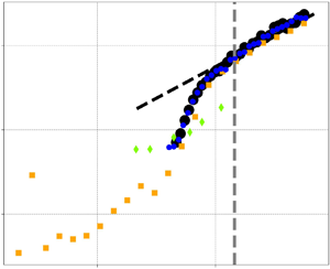
Figures 7 and 8 present the 3-D  $Nu$ versus $Ra$,
$Ra$,  $\Pr$ scalings. Figures 9 and 10 present the 3-D $Re$ versus $Ra$,
$Ra$,  $\Pr$ scalings. Scalings are always displayed both directly and in compensated form.

Figure 7. Non-dimensional heat transfer  $Nu$ versus Rayleigh number $Ra$ in three dimensions for $\Pr =1$. Correspondence between symbols and datasets is given in table 3. The grey dashed line separates the non-universal (left) and the universal (right) friction-dominated regimes for data corresponding to figure 5. (a) Plot of $Nu$ versus $Ra$. The black dashed line corresponds to $Nu\sim \sqrt {Ra}$, corresponding to asymptotic ultimate regime scaling. (b) Compensated plot $Nu/\sqrt {Ra}$ versus $Ra$.
$Ra$.

Figure 8. Scaling of non-dimensional heat transfer  $Nu$ as a function of Prandtl number $\Pr$ in three dimensions for $Ra=10^8$. Correspondence between symbols and datasets is given in table 3. The grey dashed line separates the non-universal (left) and the universal (right) friction-dominated regimes for data corresponding to figure 5. (a) Plot of $Nu$ versus $\Pr$. The black dashed line corresponds to $Nu\sim \sqrt {\Pr }$, corresponding to asymptotic ultimate regime scaling. (b) Compensated plot $Nu/\sqrt {\Pr }$ versus $\Pr$.

Figure 9. Scaling of Reynolds number  $Re$ as a function of Rayleigh number $Ra$ in three dimensions for $\Pr =1$. Correspondence between symbols and datasets is given in table 3. The grey dashed line separates the non-universal (left) and the universal (right) friction-dominated regimes for data corresponding to figure 5. (a) Plot of $Re$ versus $Ra$. The black dashed line corresponds to $Re\sim \sqrt {Ra}$, corresponding to asymptotic ultimate regime scaling. (b) Compensated plot $Re/\sqrt {Ra}$ versus $Ra$.
$Ra$.

Figure 10. Scaling of Reynolds number  $Re$ as a function of Prandtl number $\Pr$ in three dimensions for $Ra=10^8$. Correspondence between symbols and datasets is given in table 3. The grey dashed line separates the non-universal (left) and the universal (right) friction-dominated regimes for data corresponding to figure 5. (a) Plot of $Re$ versus $\Pr$. The black dashed line corresponds to $Re\sim 1/\sqrt {\Pr }$, corresponding to ultimate regime scaling. (b) Compensated plot $Re/(1/\sqrt {\Pr })$ versus $\Pr$.
At low  $Ra$, we first observe a transition from a laminar regime, where $Nu=1$, up to a turbulent regime starting around $Ra\sim 10^7$ at $\Pr =1$. In this transition regime, the Nusselt number varies approximately like $Nu\sim Ra^{2/3}$, while the Reynolds number remains less than $10^4$, but follows approximately $Re\sim Ra^{1/2}$. In this regime, the friction is negligible, as we saw, so that it corresponds to a laminar, frictionless regime.
After this laminar regime, we obtain a turbulent regime around  $10^7< Ra$ for $\Pr =1$ in which $Nu\sim Ra ^{1/2}$ and $Re\sim Ra ^{1/2}$, like GL theory. The exact value of the exponent is provided in table 1. In this regime, the friction is non-negligible, so that it is a ‘turbulent friction-dominated regime’. However, as both ratios $f_u=fU^2_{ls}/\epsilon _u$ and $f_\theta =f\varTheta ^2_{ls}/\epsilon _{\theta }$ remain independent of $Ra$, they do not change the scaling of the total kinetic and thermal energy dissipation. Therefore, the argument developed by GL theory should still apply in this situation, as is indeed observed, with minor corrections due to the small variations of the ratios.
In that respect, it is not surprising that the the extent of this regime varies with  $\Pr$, as is shown in figure 11 for various $Ra$. At $Ra=10^8$, the ‘universal GL’ regime stops for $\Pr <\sim 10^{-1}$. In this range of parameters, $Re$ is still large, so that the flow is turbulent. However, $Nu$ drops quicker with decreasing $\Pr$ than in the universal GL regime, as can be seen from the filled data points in figure 8, in parallel with a similar drop for the thermal friction observed in figure 5(b). This regime seems therefore dependent on the variation in the friction, and is non-universal. In this regime, the Reynolds number variation with $\Pr$ is milder than in the universal regime, as can be seen in figure 10.

Figure 11. Scaling of heat transfer  $Nu$ as a function of Prandtl number $\Pr$ in 3-D results at fixed $Ra$, dataset VII (table 3). Plots of (a) $Nu/\sqrt {\Pr }$ versus $\Pr$ for various $Ra$ and (b) $Re/(1/\sqrt {\Pr })$ versus $\Pr$ for various $Ra$.
$Ra$.
As the Rayleigh number increases, we nevertheless observe in figure 11 that the extent of the universal turbulent regime extends towards smaller and smaller values of  $\Pr$, so that the universal scaling regime corresponds to an ‘asymptotic scaling regime’ at low value of $\Pr <1$, valid in the limit of infinite $Ra$.
$Ra$.
Figures 12 and 13 plot the kinetic and thermal dissipation rates  $\epsilon _u,\epsilon _\theta$ against GL predictions. In agreement with what has been observed previously, we observe agreement with GL theory in the range of parameters where the friction ratios are approximately constant with the parameters, i.e. at large value of $Re \Pr$. Overall, it is interesting to note that even when the friction is dominant, we can recover the ultimate regime scaling, as long as the velocity friction ratio remains relatively constant as a function of the parameters and that there is not too large an asymmetry between the two frictions. In regimes where the asymmetry prevails, there are no clear scaling laws that emerge, meaning that the scalings are probably not universal in $Ra$ and $\Pr$ only, and that friction-depending corrections need to be implemented.

Figure 12. Scaling of thermal dissipation rate  $\epsilon _\theta$ compared with the GL prediction $Re\sqrt {\Pr /Ra}$ in 3-D results. Correspondence between symbols and datasets is given in table 3. The grey dashed line separates the non-universal (left) and the universal (right) friction-dominated regimes for data corresponding to figure 5. (a) Plot of $\epsilon _\theta \sqrt {Ra\Pr }$ versus $Re\Pr$. The black dashed line corresponds to the GL prediction $\epsilon _\theta \sim Re (\Pr /Ra)^{1/2}$. (b) Compensated plot $\epsilon _\theta \sqrt {Ra\Pr }/\sqrt {Re\Pr }$ versus $\sqrt {Re\Pr }$.

Figure 13. Scaling of kinetic dissipation rate  $\epsilon _u$ compared with the GL prediction $Re^3(\Pr /Ra)^{3/2}$ in 3-D results. Correspondence between symbols and datasets is given in table 3. The grey dashed line separates the non-universal (left) and the universal (right) friction-dominated regimes for data corresponding to figure 5. (a) Plot of $\epsilon _u\sqrt {Ra^3\Pr }$ versus $Re^3\Pr ^2$. The black dashed line corresponds to the GL prediction $\epsilon _u\sim Re ^3(\Pr /Ra)^{3/2}$. (b) Compensated plot $\epsilon _u\sqrt {Ra^3\Pr }/Re^3\Pr ^2$ versus $Re^3\Pr ^2$.
4. Conclusion
In this paper, we investigated scaling laws in the HRB equations through a new mathematical framework (log-lattice). Using a modified DOPRI solver, we are able to explore a range of parameters and wavenumbers way beyond what is accessible in DNS of the equations. By adding a large-scale friction to the HRB equations, we are able to solve the issue of exponentially diverging solutions. This large-scale friction becomes non-negligible when the fluid becomes turbulent enough, so that the total energy balance departs from the energy balance considered in GL theory, where no friction is present. Despite this, we still observe scaling laws for  $Nu$ and $\Pr$ that are very close to the universal turbulent predictions of GL theory: $Nu\sim Ra ^{1/2}\Pr ^{1/2}$, $Re\sim Ra ^{1/2}\Pr ^{-1/2}$, $\epsilon _\theta \sim Re (\Pr /Ra)^{1/2}$, $\epsilon _u\sim Re ^3(\Pr /Ra)^{3/2}$ for an important range of parameters, corresponding to situations where the thermal friction is non-negligible and the kinetic friction does not vary significantly as a function of the parameters. This is obtained at large enough $Ra$ and for $\Pr$ depending on the value of $Ra$.
$Ra$.
In addition to this regime, we also observe another turbulent friction-dominated regime at  $\Pr \ll 1$. This regime has no simple and universal dependence on the parameters, and depends on the variations of the kinetic friction with the parameters.
Our observations show that the inclusion of friction, which is necessary to obtain stationary regimes in the HRB framework, makes more complex the phase space but nevertheless allows for the existence of a universal turbulent regime, where scaling laws are very close to the GL frictionless theoretical laws. In some geophysical or astrophysical situations, large-scale friction arises due to rotation (Ekman friction), stratification (Rayleigh friction) or magnetic field (Hartman friction), and the two scaling regimes we find (one universal and one non-universal) may be relevant and could be explored within the log-lattice framework.
More generally, we believe that log-lattices, with their unique performances in terms of numerical complexity, due to a spectrally sparse representation and strong mathematical qualities, have a great potential in numerical simulations of geophysical or astrophysical flows. However, as they are still in their infancy, many different paths would benefit from being explored to better understand their strengths and weaknesses. For example, it is not yet clear how the decimation of nonlinear interaction that takes place in log-lattices influences the prefactors of the scaling law. The comparison with DNS data shown in figure 7(a) for example indicates that the log-lattice model with friction is more efficient for transporting heat than the DNS without friction. Whether this difference is due to friction or to the decimation is still an open question, and a topic of ongoing work. Another issue is whether the inclusion of rotation in log-lattices will play the same role as in DNS, as rotation is known to influence the nonlinear interactions, not the energy budget. This is left for future work. Finally, the necessity of dealing with hyper-large wavenumbers in log-lattices sets an issue as to the best numerical scheme to integrate numerically the dynamics, and include viscous effects; this is discussed in the supplementary material, and we are currently exploring whether methods such as discussed in Whalen, Brio & Moloney (Reference Whalen, Brio and Moloney2015) could prove useful in that regard. Other topics of interest include the behaviour of observables when  $\lambda \to 1$ and the addition of the $k=0$ mode would prove very interesting to study. Likewise, in a similar spirit as was done for the REWA model in Grossmann, Lohse & Reeh (Reference Grossmann, Lohse and Reeh1996), a detailed comparison of DNS and log-lattice results (which is far from trivial, as there is room for interpretation as to the mathematical meaning of the fields simulated on a log-lattice) would be highly useful.
Supplementary material
Supplementary material is available at https://doi.org/10.1017/jfm.2023.204.
Acknowledgements
We thank A. Mailybaev and C. Campolina for initiating us to the log-lattice computations, and for stimulating discussions.
Funding
This work received funding from the Ecole Polytechnique, from ANR EXPLOIT, grant agreement no. ANR-16-CE06-0006-01 and ANR TILT grant agreement no. ANR-20-CE30-0035.
Declaration of interests
The authors report no conflict of interest.


