


1. Introduction
Ice-core samples taken from depth in an ice sheet reveal strong fabrics, shown by significant alignment of initially randomly distributed c axes of individual crystals, and consequent substantial differences in shear viscosities in different planes. A macroscopic viscous law for the shear stress proposed by Reference Morland and StaroszczykMorland and Staroszczyk (1998) was motivated by a simple picture of the rotational recrystallization in which individual crystal glide planes, material planes, are rotated towards planes normal to principal axes of compression, and away from planes normal to principal axes of extension, described as the principal stretch planes. The instantaneous viscous response at each stage of the deformation has reflexional symmetry in these planes;that is, the instantaneous viscous response is orthotropic with respect to the current principal stretch planes. The directional strengths of the response depend on the current deformation. The orthotropic viscous law is then a frame- indifferent relation between deviatoric stress, strain rate, deformation and the three structure tensors defined by the outer products of the three orthogonal unit vectors along the principal stretch axes. Subsequently, a set of equalities and inequalities on the instantaneous directional viscosities was derived from the rotation concepts by Reference Staroszczyk and MorlandStaroszczyk and Morland (2000), designated by one author (L.W.M.) as the ‘Staroszczyk inequalities’, which showed that at least two tensor generators in the orthotropic law were required. Further refinements (Reference Staroszczyk and MorlandStaroszczyk and Morland, 2001; Reference Morland and StaroszczykMorland and Staroszczyk, 2003) led to a model law with two tensor generators, each with a fabric response coefficient function, but with an equality from the Staroszczyk inequalities providing an explicit relation between the two functions, so only one fabric response function need be prescribed. Two such model functions were constructed by correlation with complete (idealized) monotonic uniaxial compression and shearing responses which satisfy observed limit viscosity enhancement factors associated with cold and warm ice. The initial isotropic response enters as a multiplying factor depending on a strain-rate invariant and incorporating a temperature-dependent rate factor.
While this fabric-evolution model ignores such effects as grain growth and temperature variation during the evolution, it is adopted here to illustrate, for the first time, the possible significance of fabric effects included in the determination of an ice-sheet flow, with the cold- and warm-ice models reflecting contrasting influences. We have investigated steady radially symmetric flow to restrict the system of partial differential equations to two independent variables, horizontal and vertical spatial coordinates, which allow accurate numerical solution. This incorporates a realistic lateral spreading which is lost in the simpler plane flow equations. The adopted temperature field is prescribed in terms of surface elevation and depth below surface, such that there is uniform heat flux into the base and a constant rate of temperature decrease with elevation at the surface. The applied elevation-dependent surface accumulation/ ablation increases exponentially with elevation from large ablation at the margin to smaller accumulation at the divide. The prescribed basal sliding law is a linear relation between the basal tangential traction and velocity, with coefficient proportional to the normal traction which eliminates a surface slope singularity at the margin. The theory allows a prescribed basal melting/refreezing distribution, but this is assumed zero in the illustrations.
We also consider bed topography of modest slope relative to the horizontal mean bed plane. Reference MorlandMorland (2000) derived the enhanced reduced model for steady plane isothermal linearly viscous flow over beds of moderate slope, S, which are the leading order balances in asymptotic expansions of the full system of equations and boundary conditions, depending on the very small surface slope, є, and on the allowed larger topography slope, δ (є ≪ δ ≪ 1), and on s, the topography span relative to the sheet thickness, where 1 ≲ s ≲ 1/δ. The error magnitude is of order δ/s. The expansions were generalized for prescribed temperature and non-linear viscous flow by Reference Morland, Straughan, Greve, Ehrentraut and WangMorland (2001), obtaining the same error magnitude. We now derive the analogous leading order balances, an enhanced reduced model, with the above anisotropic viscous law incorporating fabric evolution. The error magnitude is now of order δ, which is greater than before when s ≫ 1; hence the description ‘modest slope’. Illustrations, and comparisons with the isotropic theory, are presented for both the cold- and warm-ice models, for a flat bed, a bed with a single hump of maximum slope δ = 0.01 and a bed with a single hollow of maximum slope δ = 0.01.
The numerical procedure is a non-trivial iteration between the hyperbolic partial differential equations governing the fabric evolution for a given velocity field, starting with the isotropic flow solution, and the solution of the two-point boundary-value problem given by the enhanced reduced model for the flow with given fabric. The final solution criterion is that the relative changes of margin radius, divide height and mean thickness are all less than 10-5. Full details of the numerical methods are presented in section 7.
2. Fabric Evolution Anisotropic Viscous Law
2.1. Initial isotropic response
The initial isotropic response is defined by a non-linear viscous, incompressible, fluid relation between the strain- rate tensor D and the deviatoric stress tensor σ, with a temperature-dependent rate factor a(T), where T is absolute temperature. The deviatoric stress is defined in terms of the Cauchy stress, σ, and mean pressure, p, by
where I is the unit tensor. The conventional simplifications that D is parallel to σ, and the viscosity coefficient depends only on the second principal invariant of ![]() or of D, are adopted. The equivalent stress and strain-rate formulations of the viscous law are
or of D, are adopted. The equivalent stress and strain-rate formulations of the viscous law are

where ![]() is an effective strain rate defined by
is an effective strain rate defined by
The units σ 0 and D 0 are chosen, with unit rate factor a at the melting temperature, so that the constitutive functions ψ(J) and ϕ(Ĩ) are of order unity for deviatoric stresses and strain rates arising in typical ice-sheet flows,
Given a monotonic ϕ(Ĩ) or ψ(J), there is a unique monotonic ψJ) or ϕ(Ĩ), respectively, satisfying, from (2), the relations
The pressure, p, is a workless constraint not given by a constitutive law, but determined by momentum balance and boundary conditions.
An accurate approximation to the Reference GlenGlen (1955) data over a shear stress range 0–5 × 10⁵ N m–2, 0 ≤ J ≤ 25, is given by the polynomial representation for ψJ) determined by Reference Smith and MorlandSmith and Morland (1981):
This has the mathematical advantage of a finite viscosity at zero stress, unlike the power law proposed by Reference GlenGlen (1955), and is adopted here. We will show that the enhanced reduced model in fact requires only the function ψ(J), and not ϕ(Ĩ), for the isotropic response, even though the asymptotic analysis with the anisotropic law starts from the expression for stress. They also derived an accurate representation for a(T) from data presented by Reference Mellor and TestaMellor and Testa (1969) for temperatures between melting and 60 K below melting. A good simplifying approximation of that representation over the range of practical significance from melting to 40 K below melting is

which is adopted here. The dimensionless temperature ![]() is zero at melting, and –2 at 40 K below melting.
is zero at melting, and –2 at 40 K below melting.
2.2. Orthotropic viscous law
For direct application to the momentum balances of ice- sheet flows, a constitutive law for the stress is required. The law adopted here is that proposed by Reference Morland and StaroszczykMorland and Staroszczyk (2003), in which the fabric is governed by the evolution of the left Cauchy–Green strain tensor B = FFT , where F is the deformation gradient and the superscript ‘T’ denotes transpose of a tensor. Let Ox i (i = 1,2,3) be spatial rectangular Cartesian coordinates with OXi (i = 1,2,3) particle reference coordinates, and v i the velocity components, then the deformation gradient F, spatial velocity gradient L and strain rate D have components

The kinematic relation for B is
where t denotes time and the notation D/Dt denotes a material time derivative. In practice, (9) must be solved simultaneously with the momentum balance and constitutive law, and is subject to an initial condition that B = F = I, the unit tensor, when the ice is first deposited at the surface. The orthogonal unit vectors e(l) (l = 1,2,3) defining the principal stretch axes, and the squares b l (l = 1,2,3) of the principal stretches, are defined by
The latter relation is a cubic equation with positive roots. By incompressibility,
An orthotropic, with respect to the principal stretch planes, viscous law for the deviatoric stress σ is a frame-indifferent relation depending on the strain-rate tensor D, the left Cauchy–Green strain tensor B, and three structure tensors M (l) defined by the outer products of the current principal stretch axes unit vectors e (l) (l = 1,2,3),
A key feature of the law proposed by Reference Morland and StaroszczykMorland and Staroszczyk (2003) is the choice of the invariant arguments for the two fabric response coefficient functions, for which the directional viscosity equality yields an explicit algebraic relation between the two functions. These invariants are
where
instead of the previous invariants b l and K used in earlier formulations by Reference MorlandStaroszczyk and Morland (2000, 2001). Henceforth omitting the subscript ‘l’ for common relations, the invariants have the properties

The proposed stress formulation is then

where µ is the isotropic viscosity function defined by
and ![]() and
and ![]() are the fabric response coefficients. The dependence of the coefficient
are the fabric response coefficients. The dependence of the coefficient ![]() for the term involving M
(l) on bl
alone, and the dependence of the coefficient
for the term involving M
(l) on bl
alone, and the dependence of the coefficient ![]() on an isotropic invariant, chosen to be K, were deduced (Reference Morland and StaroszczykMorland and Staroszczyk, 1998) from symmetry conditions on the directional viscosities as the bl
are permuted. Note that the law (14) makes the simplifying assumptions that the temperature influences both the rate of strain and the fabric evolution only through the effective strain rate, i.e. with a common rate factor a(T), and that the anisotropic part also has the isotropic viscosity function µ as a multiplying factor. The vanishing of the anisotropic part when B = I gives the normalization condition
on an isotropic invariant, chosen to be K, were deduced (Reference Morland and StaroszczykMorland and Staroszczyk, 1998) from symmetry conditions on the directional viscosities as the bl
are permuted. Note that the law (14) makes the simplifying assumptions that the temperature influences both the rate of strain and the fabric evolution only through the effective strain rate, i.e. with a common rate factor a(T), and that the anisotropic part also has the isotropic viscosity function µ as a multiplying factor. The vanishing of the anisotropic part when B = I gives the normalization condition
Bounded response as b
l → ∞, hence K and η → ∞, implies ![]() as η → ∞, and it is convenient to introduce the alternative fabric response function G(η) defined by
as η → ∞, and it is convenient to introduce the alternative fabric response function G(η) defined by
where ![]() is finite and non-zero as η → ∞. The non-trivial directional viscosity equality (Reference Morland and StaroszczykMorland and Staroszczyk, 2003) with this choice of invariant arguments gives an explicit relation for
is finite and non-zero as η → ∞. The non-trivial directional viscosity equality (Reference Morland and StaroszczykMorland and Staroszczyk, 2003) with this choice of invariant arguments gives an explicit relation for ![]() in terms of
in terms of ![]() namely,
namely,
where ![]() is the odd part of
is the odd part of ![]() is the even part). That is, in terms of the new invariant arguments,
is the even part). That is, in terms of the new invariant arguments, ![]() is determined explicitly in terms of
is determined explicitly in terms of ![]() and the constitutive law can be expressed directly in terms of a single independent fabric response function
and the constitutive law can be expressed directly in terms of a single independent fabric response function ![]() The limit of (18) as b
l → 1, η → 0, together with the normalization (16), shows that
The limit of (18) as b
l → 1, η → 0, together with the normalization (16), shows that

which is a restriction on ![]() at ξ = 0; the prime denotes an ordinary derivative of a function with respect to its argument.
at ξ = 0; the prime denotes an ordinary derivative of a function with respect to its argument.
2.3. Uniaxial compression and shear limits
Reference Budd and JackaBudd and Jacka (1989) and Reference Li, Jacka and BuddLi and others (1996) have experimentally determined the limit ratios of fabric-induced viscosity to isotropic viscosity for indefinite axial compression with equal unconfined lateral extensions, and for indefinite shear in a plane deformation, A and S, respectively. Since these experiments were near melting temperature, we use the term warm ice. In contrast, Reference Mangeney, Califano and CastelnauMangeney and others (1996) deduced values of A and S from the ice-core data of Reference Thorsteinsson, Kipfstuhl and MillerThorsteinsson and others (1997), for which we use the term cold ice. The reciprocals of these ratios, A¯1and S¯1, are described as enhancement factors. While the warm-ice experiments showed A to be less than unity, the cold-ice-core measurements showed A to be greater than unity. Here we adopt the parameters inferred by Reference Morland and StaroszczykMorland and Staroszczyk (2003) from the above,

The uniaxial and shear ratios given by (14) provide two more restrictions on the limit values of ![]() and
and ![]() which combine to give (Reference Morland and StaroszczykMorland and Staroszczyk, 2003)
which combine to give (Reference Morland and StaroszczykMorland and Staroszczyk, 2003)

from which, with the parameters (20),
2.4. Fabric response functions
Reference Morland and StaroszczykMorland and Staroszczyk (2003) assumed, since data for the full uniaxial and shear responses are not known, that both responses varied exponentially between their known initial and limit values, and determined a corresponding fabric function ![]() of order unity by construction, by least-squares correlation with both responses for both warm and cold ice.
of order unity by construction, by least-squares correlation with both responses for both warm and cold ice.
For warm ice, the correlation gave
where
and

For cold ice, the correlation gave

where

3. Axially Symmetric Flow
Steady axisymmetric flow of a large ice sheet is described by the radial and vertical velocity fields, u(r,z) and w(r,z), respectively, where r is a horizontal radial coordinate and z is a vertically upward distance coordinate of cylindrical polar coordinates (r, θ, z), and all the flow variables are independent of the polar angle, θ. The corresponding nonzero physical components of the strain rate are

subject to the assumption of incompressibility, equivalent to the mass-balance condition,
which is satisfied identically by expressing the velocity components in terms of a stream function, ω(r,z),
The horizontal radial and vertical momentum balances for the very slow flow in which acceleration terms are negligible are, respectively,

where ρ = 918kgm–3 is the constant ice density, g =9.81 ms–2 is the constant gravity acceleration, and the circumferential momentum balance is automatically satisfied.
It is supposed that the atmospheric pressure at the surface is uniform, and stress is measured relative to this pressure. Then the ice-sheet surface z = h(r) is traction-free, and is subjected to a normal net ice flux qn , which is positive over accumulation zones and negative over ablation zones. It is expected that accumulation will occur over a central zone at higher elevations, and ablation below a snowline. In general, qn will depend on elevation h and location r. Let the surface have unit tangent and outward normal vectors s and n in a righthand sense, then

The zero traction is conveniently expressed in terms of vanishing normal and tangential tractions t n = n ×σ× n and t s = s ×σ× n in the Orz plane,

The kinematic condition prescribing the surface accumulation flux becomes
where v
n is the normal ice velocity and ![]() is the equivalent vertical flux which can be identified with equivalent vertical snowfall. In general,
is the equivalent vertical flux which can be identified with equivalent vertical snowfall. In general, ![]() will depend on surface elevation and location, but the later illustrations assume dependence on elevation only - dependence on location only is a simpler problem, but artificial. Equation (32) is the additional boundary condition required to determine the unknown surface h(r). A prescribed temperature field incorporates a prescribed surface temperature.
will depend on surface elevation and location, but the later illustrations assume dependence on elevation only - dependence on location only is a simpler problem, but artificial. Equation (32) is the additional boundary condition required to determine the unknown surface h(r). A prescribed temperature field incorporates a prescribed surface temperature.
The bed z = f(r) is prescribed. The vectors s and n are defined by

Normal and tangential tractions t n and t s are given by

and normal and tangential velocities v n and v s by
The kinematic condition prescribing the normal basal melt flux, bn, negative if freezing occurs, is
A linear sliding relation between the tangential traction and velocity is assumed, given by
where γ is a friction coefficient depending in general on the overburden pressure –t n. The proportionality of t s to t n ensures bounded surface slope at the margin where the ice thickness, and overburden pressure, approach zero (Reference Morland and JohnsonMorland and Johnson, 1980). The case of no-slip gives rise to unbounded surface slope at a margin at which there is ablation in the reduced model (Reference Morland and JohnsonMorland and Johnson, 1980; Reference MorlandMorland, 1997), which violates the expansion scheme. Figure 1 shows an ice-sheet profile with the above conditions displayed, and gives notation for physical coordinates, velocity components and the later dimensionless variables.

Fig. 1. Ice-sheet geometry.
4. Enhanced Reduced Model
We now introduce typical magnitudes for the physical variables so that normalized dimensionless variables can be defined. Let d 0 be a thickness magnitude and q 0 a vertical velocity magnitude, defined by a typical surface accumulation, then pgd 0 is an overburden pressure magnitude, d0/q0 is a flow time magnitude and q 0/d 0 is a vertical strain-rate magnitude. Typical values are adopted here,
then

Define

then Z, H, P, Q, B are order unity variables, F is of order of its amplitude, ĸ, which may be order unity or less, and W is yet to be estimated. The viscous law (14) now becomes

where ![]() is defined by
is defined by
and with the chosen parameters,
We formally treat the product ![]() as an order unity quantity, since it was noted by Reference Morland and SmithMorland and Smith (1984) that as a(T) becomes small in cold upper regions of an ice sheet, so does the strain rate. є2 is the magnitude of the dimensionless viscosity in law (42).
as an order unity quantity, since it was noted by Reference Morland and SmithMorland and Smith (1984) that as a(T) becomes small in cold upper regions of an ice sheet, so does the strain rate. є2 is the magnitude of the dimensionless viscosity in law (42).
In the reduced model, leading order equations are developed by introducing the coordinate and variable stretchings
where R, U and Ω are order unity, and

We are allowing a bed topography with modest slope δ, and with amplitude k and span ĸ relative to the thickness d 0, where
as treated by Reference Morland, Straughan, Greve, Ehrentraut and WangMorland (2000, 2001) and Reference Cliffe and MorlandCliffe and Morland (2002). Due to the bed topography, variables change with r over a dimensionless length scale s near the bed, so that ![]() derivatives leave the order unchanged. Thus F’(R) is order ĸ/(єs) = S/є ≫ 1, and it follows from the basal melt condition (36) that W is also that order. All R derivatives of order unity variables will be of order (єs)–1, with higher derivatives multiplied successively by this factor. We expect the surface to vary on the R scale, i.e. the scaled surface slope H′(R) = Γ(R) to be order unity, but will allow it to be as great as the scaled bed slope F′(R) = ß = O(δ/є) in the later asymptotic expansions. For valid expansions at the margin, it must be assumed that the bed slope in a margin region must not be greater than є in magnitude, and hence F’(R) is order unity there. The analysis for the isotropic viscous law shows that the error of the enhanced reduced model is of order δ/s. We will now show that with the anisotropic viscous law (42) the error becomes of order S, which is greater when s ≫ 1.
derivatives leave the order unchanged. Thus F’(R) is order ĸ/(єs) = S/є ≫ 1, and it follows from the basal melt condition (36) that W is also that order. All R derivatives of order unity variables will be of order (єs)–1, with higher derivatives multiplied successively by this factor. We expect the surface to vary on the R scale, i.e. the scaled surface slope H′(R) = Γ(R) to be order unity, but will allow it to be as great as the scaled bed slope F′(R) = ß = O(δ/є) in the later asymptotic expansions. For valid expansions at the margin, it must be assumed that the bed slope in a margin region must not be greater than є in magnitude, and hence F’(R) is order unity there. The analysis for the isotropic viscous law shows that the error of the enhanced reduced model is of order δ/s. We will now show that with the anisotropic viscous law (42) the error becomes of order S, which is greater when s ≫ 1.
First we must estimate the magnitudes of the dimensionless scaled stress components and their derivatives which appear in the momentum balances and boundary conditions. Note that all components of ![]() never exceed unity in magnitude because of property (17) and definition (13). Immediately from (46),
never exceed unity in magnitude because of property (17) and definition (13). Immediately from (46), ![]() but
but ![]() and
and ![]() are greater than order unity, so by the incompressibility condition (27) their leading order terms must be equal and opposite, namely of order (єs)–1. This implies that where R derivatives need the factor (єs)–1 near the bed, Z derivatives are increased by the factor ĸ¯1 to reflect the topography effects, and are therefore of order є/S smaller than the corresponding R derivative. Thus, from (46),
are greater than order unity, so by the incompressibility condition (27) their leading order terms must be equal and opposite, namely of order (єs)–1. This implies that where R derivatives need the factor (єs)–1 near the bed, Z derivatives are increased by the factor ĸ¯1 to reflect the topography effects, and are therefore of order є/S smaller than the corresponding R derivative. Thus, from (46),

The relation ![]() applies throughout the depth, even when Z derivatives away from the bed leave magnitudes unchanged. Further, the order of the R derivative of W in
applies throughout the depth, even when Z derivatives away from the bed leave magnitudes unchanged. Further, the order of the R derivative of W in ![]() is a factor δє or δ2, near or away from the bed, respectively, of the Z derivative of U.
is a factor δє or δ2, near or away from the bed, respectively, of the Z derivative of U.
All components of each M (l) are order unity. Define

Note that e
(2) = (0,1,0), so that for l = 1,3, ![]() = 0, and
= 0, and

The non-zero component of A (2) is
and for l = 1,3 the non-zero components of A (l) are

all dominated by ![]() with relative error of order δ by (49).
with relative error of order δ by (49).
The non-zero components of C are

where the product ![]() does not exceed unity in magnitude, so again all components are dominated by
does not exceed unity in magnitude, so again all components are dominated by ![]() with relative error of order δ.
with relative error of order δ.
The usual scaled dimensionless deviatoric stress, ![]() is defined by
is defined by
then from (42), (49), (50) and (52–54),

all with relative error δ at most, where
The expressions for crz and czz are order unity with relative error δ. Then the shear stress invariant, J, defined in (2), becomes

with the chosen parameters (4), (38) and (39). With the isotropic viscous law, crz ≡ 1, czz ≡ 0. By (49), ![]() is of order (δєs)–1, and hence the deviatoric stress
is of order (δєs)–1, and hence the deviatoric stress ![]() components given by (42) are of order є/(δs), which is much smaller than unity in view of the strong inequalities (48);in fact, not greater than δ if we assert s ≳ єδ–2, which is a reasonable restriction, consistent with (48), and is assumed here. Now all the components of
components given by (42) are of order є/(δs), which is much smaller than unity in view of the strong inequalities (48);in fact, not greater than δ if we assert s ≳ єδ–2, which is a reasonable restriction, consistent with (48), and is assumed here. Now all the components of ![]() are order δ/є.
are order δ/є.
From (30) and (33) it follows that ∆h and ∆f are both unity, with maximum error δ2, so from (31) and (32) the surface conditions become, to lead order, neglecting terms of order δ,
Similarly, neglecting order δ terms, on the bed, from (34) and (35),

so that the basal boundary conditions (from (36) and (37)) become

and we suppose Λ is order unity or greater. The momentum
balances (29) are exactly


Since the components of ![]() are at most of order δ/є, and recalling the deduction above Equation (49) that R derivatives are not greater than a factor δ/є of Z derivatives, the leading order balances of (63) and (64), neglecting terms of order δ in the former, and order δ and δ2 in the latter, become
are at most of order δ/є, and recalling the deduction above Equation (49) that R derivatives are not greater than a factor δ/є of Z derivatives, the leading order balances of (63) and (64), neglecting terms of order δ in the former, and order δ and δ2 in the latter, become

Equations (60), (62) and (65) are those of the enhanced reduced model, but the fabric changes the deviatoric stress expressions (56) and the invariant J defined by (59) through the factors c rz, c zz and c defined by (57) and (58).
5. Flow Solution
Here we decouple the radial flow boundary-value problem defined by (55–59), (60), (62) and (65) from the fabric evolution, by assuming that the fabric through the ice-sheet domain is known;that is, crz(r,z) defined by (57), czz(r,z) defined by (58) and c(r,z) defined by (59) are given functions. Subsequently we solve the fabric-evolution equations assuming that the velocity field is known, and then construct the coupled flow by an iteration procedure. ![]() is defined by (43) with a(T) given by (7) and ψ(J) by (6). Solutions of the momentum balances (65) subject to the surface conditions (60), and the invariant J defined by (59), have the simple expressions
is defined by (43) with a(T) given by (7) and ψ(J) by (6). Solutions of the momentum balances (65) subject to the surface conditions (60), and the invariant J defined by (59), have the simple expressions

Denote basal values on Z = F(R) by a subscript ‘b’, then by (66) and (62),

where ∆(R) is the ice thickness at R. From (57), (60), (67) and (47),
Integrating twice with respect to Z,


Now the surface accumulation condition (60) and basal melt condition (62) with the relations (47) become

where subscript ‘s’ denotes evaluation on the surface Z = H(R). Differencing the relations in (72), and evaluating Ωs by (70), gives

where U b is given by (67) in terms of Γ(R) and Λ(D), and

and g and g2s depend on Γ, hence dg2s/dR includes Γ’(R). It follows that (73) is a second-order differential equation for H(R).
This differential equation applies over an unknown span, the margin radius R M, which must be determined as part of the flow solution. The subscript ‘M’ will denote evaluation at the margin. In section 7 the explicit second-order equation for H(R) will be transformed into an equivalent system of first-order equations, and an asymptotic limit for Γ’(R) as R → 0, since Γ’(R) is indeterminate at the divide, will be given (see (90)). As R → RM , so Δ → 0, and recalling the assumption that ß is order unity near the margin, an asymptotic analysis (Reference MorlandMorland, 1997) determines both ΓM and ΓM in terms of RM and prescribed functions evaluated at R M; thus

Note that ΓM
< ß
M for positive thickness inside the margin, so the Γ′м factor is non-zero, and ![]() and
and ![]() denote derivatives with respect to R, and not their given arguments. While the second-order equation could be integrated from the margin for a sequence of trial R
м, with the margin slope given by (76), until the R
м is found such that the surface slope becomes zero at R = 0, the indeterminancy there in Γ′ is not given by the finite asymptotic limit for each incorrect trial Rм, and the numerical procedure is unstable (Reference MorlandMorland, 1997). The stable approach (Reference Cliffe and MorlandCliffe and Morland, 2002) treats the problem as a two-point boundary-value problem with both Rм and the divide elevation H(0) = H
D as unknown parameters, where the subscript ‘D’ denotes evaluation at R = 0. The differential equation is integrated from both the margin where H = F and H′ = Γм, and from the divide, R = 0, where H = H
D and H′ = 0, for a sequence of trial R
м and H
D until both surface elevation H and slope Γ match at a chosen interior radius. The method is described further in section 7. Once the profile H(R) with R
м and H
D are determined, the velocity fields and derivatives can be determined to apply to the fabric-evolution equations.
denote derivatives with respect to R, and not their given arguments. While the second-order equation could be integrated from the margin for a sequence of trial R
м, with the margin slope given by (76), until the R
м is found such that the surface slope becomes zero at R = 0, the indeterminancy there in Γ′ is not given by the finite asymptotic limit for each incorrect trial Rм, and the numerical procedure is unstable (Reference MorlandMorland, 1997). The stable approach (Reference Cliffe and MorlandCliffe and Morland, 2002) treats the problem as a two-point boundary-value problem with both Rм and the divide elevation H(0) = H
D as unknown parameters, where the subscript ‘D’ denotes evaluation at R = 0. The differential equation is integrated from both the margin where H = F and H′ = Γм, and from the divide, R = 0, where H = H
D and H′ = 0, for a sequence of trial R
м and H
D until both surface elevation H and slope Γ match at a chosen interior radius. The method is described further in section 7. Once the profile H(R) with R
м and H
D are determined, the velocity fields and derivatives can be determined to apply to the fabric-evolution equations.
6. Fabric Evolution
Now we assume that the domain and velocity fields and derivatives required in the evolution equations for B are known. Let ![]() be a dimensionless time with unit d
0/q
0, then the kinematic relation (9) gives the non-zero relations
be a dimensionless time with unit d
0/q
0, then the kinematic relation (9) gives the non-zero relations

The relations are retained in full since some components of B increase indefinitely as the stretches normal to the dominant compression increase indefinitely; we cannot set bounds. The incompressibility condition (11) is satisfied identically by using
and ignoring the evolution equation for Bzz . It is expected that B rr ≥ B θ ≥ 1, and Bzz ≤ 1, or close to this situation, and both Brr and Bθθ will approach infinity, and Bzz will approach zero, as the ice is compressed vertically as it approaches the bed, while Brz , zero in the undeformed state, may be positive or negative as the ice flows through the sheet, but not greater in magnitude than B rr. Numerical solution is most sensibly conducted in order unity variables, and after some trials we found that introducing the following normalized variables yielded satisfactory evolution equations,

The three evolution equations for ζ1, ζ2 and ζ3, by (78), are

where, in steady flow, the material time derivative reduces to the convective terms
for all ζ, and by the incompressibility relation (79),
7. Numerical Method
We apply the following iteration procedure. First solve the flow problem for the profile and velocity field, and the strain-rate components and velocity derivative ∂W/∂R which are required in the fabric-evolution equations (81), for a given fabric distribution defined by functions crz (r,z) and c zz r,z). Then solve the fabric-evolution problem with this flow field to determine new fabric functions crz (r,z) and czz(r,z), which are then used to solve a new flow problem, and continue this sequence. We start by solving the flow problem with isotropic ice for which crz (r,z) ≡ 1 and
czz(r,z) ≡ 0, and continue the iteration until the final flow solution profile is sufficiently close to the previous one. To move between the two problems – a second-order ordinary differential equation with two end-point boundary conditions, on an unknown span R M changing at each iteration, and the hyperbolic partial differential equations governing the fabric evolution – we map each ice-sheet domain in the sequence on to the same fixed domain, a unit square. Introducing new variables (t,y) by the transformations

the surface Z = H(R) becomes y = 0, the bed Z = F(R) becomes y = 1, and the divide R = 0 becomes t = 0. The margin R = R M, where the thickness Δ(RM) = 0, is expanded to 0 < y < 1 at t = 1, but no depth integrals in the flow equations are required when Δ(R) = 0. It is supposed that there is a single snowline in the later illustrations, at tE, so that there is surface accumulation for 0 ≤ t < t E and surface melt for t E < t < 1; that is

The mapped domain and a typical ice particle path are shown in Figure 2.

Fig. 2. Typical ice particle path in the (t,y) domain.
With the change of variables

the second-order differential equation defined by (73–75), with definition (71) for g2(R,Z), and unknown parameters RM and H
D, can be expressed as four first-order differential equations for ![]() R
M and H
D:
R
M and H
D:

subject to the boundary conditions

where ΓM is given by (76). The complexity lies in the surface slope derivative given by
where

and
The integrand functions of (R,Z) must be transformed to (t,y) dependence before integration, and in particular the partial derivative ∂c/∂R at constant Z must be expressed in terms of partial derivatives with respect to t and γ, then the latter is integrated out by parts.
The expression (89) for G is indeterminate as t → 0 at the divide, and as t → 1 when ![]() at the margin. The latter asymptotic limit is simply
at the margin. The latter asymptotic limit is simply ![]() , where ΓM is given by (76). The former asymptotic limit is
, where ΓM is given by (76). The former asymptotic limit is
The velocity fields U and W are then given by (47), and the strain-rate components, required by the fabric-evolution equations (81), are given by (46) and (56) with Ω given by (70). These involve integrals from y- to 1 at ti for each mesh point (t i,yj ). In addition, (81) requires the velocity derivative ∂W/∂R at constant Z, which is determined numerically by cubic expansions of W in the t and y directions using values at (ti ,yj ) and three adjacent points.
A uniform mesh is placed on the square with n intervals of length h
t in the t direction, and m intervals of length h
y in the y direction, defining mesh points (ti,yj
), (i = 0, ...,n; j= 0, ...,m). Given that the fabric-evolution solution has determined crz, czz and hence c, at each mesh point (ti
,yj
), the required t derivatives are obtained by cubic interpolation based on four adjacent mesh points in the t direction. For the flow problem, the depth integrations are performed using a trapezoidal approximation, with error ![]() and the differential equations (88) are solved using a second-order Runge–Kutta scheme with error
and the differential equations (88) are solved using a second-order Runge–Kutta scheme with error ![]() Newton’s root-finding method is used to determine the parameters R
M and H
D which match the surface elevation and slope at the interior point t = 0.5. Using double precision, the matching error for all the later examples was initially of order 10–8, retaining eight decimal places in R
M and H
D, but the final solutions were obtained retaining only six decimal places. The iteration between flow and fabric evolution was continued until a measure of the change from the previous flow solution defined by
Newton’s root-finding method is used to determine the parameters R
M and H
D which match the surface elevation and slope at the interior point t = 0.5. Using double precision, the matching error for all the later examples was initially of order 10–8, retaining eight decimal places in R
M and H
D, but the final solutions were obtained retaining only six decimal places. The iteration between flow and fabric evolution was continued until a measure of the change from the previous flow solution defined by

was acceptably small, where [ ] denotes the jump from the previous solution in the iteration sequence. In all the later examples er did not exceed order 10–5, and the rate of decrease in the later stages suggested that a further iteration would have yielded a much smaller value, so this final solution can be expected to change less than 10–5 with a further iteration.
Figure 2 shows a typical particle path in the (t, y) domain, starting from an accumulation point on the surface (t
s,0), where 0 < t
s < t
E, and returning to the surface at an ablation point (t
r,0) where t
E < t
r < 1. Let ![]() for all ζ, and let s denote arc length on a particle path in the (t, y) domain defined by
for all ζ, and let s denote arc length on a particle path in the (t, y) domain defined by ![]() , for which
, for which

The fabric-evolution equations (81), with the relation (82), now become


(92–94) are five ordinary differential equations for ![]() subject to the initial surface conditions at s = 0 on y = 0, t = t
s where 0 ≤ t
s ≤ t
E,
subject to the initial surface conditions at s = 0 on y = 0, t = t
s where 0 ≤ t
s ≤ t
E,
Values of ![]() to
to ![]() and in turn the values of crz
, czz
, c and their derivatives, must be determined at each mesh point (t
i,y
j), where they are required for the subsequent flow solution.
and in turn the values of crz
, czz
, c and their derivatives, must be determined at each mesh point (t
i,y
j), where they are required for the subsequent flow solution.
The divide t = 0 is a particle path with s = y, but as t → 0, so does U, ![]() and
and ![]() and hence y
d → ∞ when W ≠ 0, but
and hence y
d → ∞ when W ≠ 0, but

and ν is bounded. On t = 0, ![]() (positive),
(positive), ![]() and we suppose the bed slope does not exceed order є near the divide, so the derivative ∂W/∂R is order unity there. Then, neglecting the term of order є, the three non-trivial equations for
and we suppose the bed slope does not exceed order є near the divide, so the derivative ∂W/∂R is order unity there. Then, neglecting the term of order є, the three non-trivial equations for ![]() to
to ![]() on the divide become
on the divide become

which can be integrated numerically. However, if W→ 0 as well, then y
d is indeterminate, as is the case in our later examples which assume zero basal melting, and hence W = 0 at the base of the divide. However, the ν limit given in (95) is still the correct asymptotic behaviour, the other terms of yd being smaller, and since ![]() is positive, then
is positive, then ![]() is negative by incompressibility, and hence W behaves like –(1 – y) and ν like (1 – y)–1, positive, as y → 1. Immediately
is negative by incompressibility, and hence W behaves like –(1 – y) and ν like (1 – y)–1, positive, as y → 1. Immediately ![]() so
so ![]() behaves like a positive power of (1 – y), and
behaves like a positive power of (1 – y), and ![]() like a larger positive power of (1 – y), so B
rr → ∞, B
rz
→ 0 and B
zz
→ 0, by incompressibility. On the divide, the unit vectors e
(l) are along the coordinate axes so b
1 = B
rr, b
2 = B
θθ, b
3 = B
zz, and hence, by (13), ξ1 → ∞, ξ3 → –∞, η ~ K ~ 2b1 → ∞, and by (12) each
like a larger positive power of (1 – y), so B
rr → ∞, B
rz
→ 0 and B
zz
→ 0, by incompressibility. On the divide, the unit vectors e
(l) are along the coordinate axes so b
1 = B
rr, b
2 = B
θθ, b
3 = B
zz, and hence, by (13), ξ1 → ∞, ξ3 → –∞, η ~ K ~ 2b1 → ∞, and by (12) each ![]() is zero. Thus by (21), (57) and (58),
is zero. Thus by (21), (57) and (58),
This asymptotic limit is approached smoothly by the numerical integration to the last point before the bed y = 1. The bed is also a particle path when B = 0, but direct numerical integration in s = t from the margin is not possible because of the singular, but not explicit, behaviour of ν there.
The first approach was to integrate the five differential equations for ![]() to
to ![]() from the surface mesh points on (0,tE) using a second-order Runge–Kutta method with integration interval ht
, until the closest point to (t
r,0) was reached. Values at each mesh point were then interpolated by using nine or ten closest path points in both rectangular and polar expansions. It was found that all such interpolations became erratic in some neighbourhoods of the bed, y = 1, which we believe is because the paths become parallel and bunch close together there.
from the surface mesh points on (0,tE) using a second-order Runge–Kutta method with integration interval ht
, until the closest point to (t
r,0) was reached. Values at each mesh point were then interpolated by using nine or ten closest path points in both rectangular and polar expansions. It was found that all such interpolations became erratic in some neighbourhoods of the bed, y = 1, which we believe is because the paths become parallel and bunch close together there.
An accurate method is to integrate the path equations (92) for ![]() and
and ![]() backwards from each mesh point (t
i,yj
), to determine the corresponding start value t
s on y = 0. The final value is determined by using repeated tangent extrapolations over shorter intervals from the last point before the line y = 0 is crossed, stopping when the last interval is less than 10–6. Then all five evolution equations (92) and (93) are integrated forward from (t
s,0) to (t
i,y
j). The high accuracy is confirmed by the accurate return to (t,•,yj). With the necessarily fine mesh using second-order integration routines, computing time for the reverse and return integrations for the large number of mesh points is extremely large (many hours on an Apple G4), and must be repeated many times for the iteration between evolution and flow. An alternative strategy was therefore devised. The backward integration from each (ti,yi
) was performed to determine the point (t0,y0
) where the path first crossed a previous mesh line: t = ti–1
or y = yj–1 or y = yj+1; the four possibilities are shown in Figure 2 with typical mesh points denoted by a cross and the previous mesh line intersections by circled points. The above tangent extrapolation method was again used to determine accurate (t0,y0). The values of
backwards from each mesh point (t
i,yj
), to determine the corresponding start value t
s on y = 0. The final value is determined by using repeated tangent extrapolations over shorter intervals from the last point before the line y = 0 is crossed, stopping when the last interval is less than 10–6. Then all five evolution equations (92) and (93) are integrated forward from (t
s,0) to (t
i,y
j). The high accuracy is confirmed by the accurate return to (t,•,yj). With the necessarily fine mesh using second-order integration routines, computing time for the reverse and return integrations for the large number of mesh points is extremely large (many hours on an Apple G4), and must be repeated many times for the iteration between evolution and flow. An alternative strategy was therefore devised. The backward integration from each (ti,yi
) was performed to determine the point (t0,y0
) where the path first crossed a previous mesh line: t = ti–1
or y = yj–1 or y = yj+1; the four possibilities are shown in Figure 2 with typical mesh points denoted by a cross and the previous mesh line intersections by circled points. The above tangent extrapolation method was again used to determine accurate (t0,y0). The values of ![]() at (t
0,y0) are determined by quadratic interpolation using values at three appropriate adjacent mesh points, then the five equations are integrated forward to (ti,yj). The different possible configurations for the location of the point (t
0,y
0), which require known values at different sets of adjacent mesh points, complicates the procedure for covering the domain to provide all required values for the interpolations, but this strategy has proved very fast and accurate. The accuracy is confirmed by applying the full reverse and return integrations to selected sets of mesh points: adjacent to the divide, adjacent to the bed, and in the ablation zone of the surface;in particular the bed neighbourhood could be expected to yield the worst errors. In all the later examples, it was only at a few places in the bed, towards the margin, that significant differences arose, up to a few per cent in small zones, but these should make little difference to the depth integrals in the flow equations. The solution for mesh points on the bed was obtained by integrating the five differential equations from a surface point (10–7,0) for which the particle hugs the divide, bed and expanded margin line, and linearly interpolating between values at integration points t on either side of ti. The final values at (1,0) are used for the complete line t = 1, 0 ≤ y ≤ 1, since this is the expanded margin.
at (t
0,y0) are determined by quadratic interpolation using values at three appropriate adjacent mesh points, then the five equations are integrated forward to (ti,yj). The different possible configurations for the location of the point (t
0,y
0), which require known values at different sets of adjacent mesh points, complicates the procedure for covering the domain to provide all required values for the interpolations, but this strategy has proved very fast and accurate. The accuracy is confirmed by applying the full reverse and return integrations to selected sets of mesh points: adjacent to the divide, adjacent to the bed, and in the ablation zone of the surface;in particular the bed neighbourhood could be expected to yield the worst errors. In all the later examples, it was only at a few places in the bed, towards the margin, that significant differences arose, up to a few per cent in small zones, but these should make little difference to the depth integrals in the flow equations. The solution for mesh points on the bed was obtained by integrating the five differential equations from a surface point (10–7,0) for which the particle hugs the divide, bed and expanded margin line, and linearly interpolating between values at integration points t on either side of ti. The final values at (1,0) are used for the complete line t = 1, 0 ≤ y ≤ 1, since this is the expanded margin.
8. Illustrations
A temperature distribution used by Reference MorlandMorland (1997) is adopted,

where H and Δ denote H(R) and Δ(R), respectively, which depends on surface elevation and depth below the surface. The corresponding thermal boundary conditions are

with the realistic properties that the surface temperature decreases at a rate of 0.8 K per 100 m rise, and that there is a uniform heat flux into the base equivalent to a temperature gradient of 0.5 K per 100 m, and the Laplacian of T, arising in the energy balance, is bounded.
The surface accumulation/ablation distribution adopted is an elevation-dependent example with large margin ablation, –Q M, used by Reference MorlandMorland (1997),

with a decay height scale H = 0.25 corresponding to h = 500m. The equilibrium height (snowline) where Q = 0 is at H = 0.64 corresponding to h = 1280 m. Reference Cliffe and MorlandCliffe and Morland (2004) have investigated the dynamic stability of radial flow for linearly viscous ice with varying weighting of the accumulation dependence on elevation and location, and demonstrate in particular that dependence on elevation alone is unstable. However, direct solution of the steady flow equations with this function has always proved numerically stable, and it describes a simple, physically plausible distribution. The basal melting B ≡ 0, and a constant friction coefficient Λ ≡ 25, are adopted in all the examples presented.
We compare solutions for a flat bed, for a bed with a single symmetric hump of amplitude 0.4, corresponding to 800 m, maximum slope δ = 0.01, and slope span s = 40, corresponding to 80 km, centred at R c = 0.4, corresponding to r c = 479 km, and for a single symmetric basin which is the image of the above hump. All three cases are described by the smooth bed form

with
where the R span of the slope sections is e, and of the flat section is 2e, and ![]() is a monotonic polynomial
is a monotonic polynomial
F(R) and its first three derivatives are continuous at R
c–2e, Rc–e, Rc
+ e and Rc
+ 2e, and F(R) has a maximum slope at χ = 0.5 and ![]() where
where
with the chosen parameters, corresponding to a maximum physical slope δ = 0.01 and a hump/basin spanning 174 km. The flat, hump and basin topographies are given, respectively, by κ = 0, 0.4 and –0.4.
The solution computations were performed on a mesh with n = m = 1000 so that h
t = h
y = 0.001. In all three cases, the fabric parameter czz
remained very small, not exceeding a few per cent, so the parameter c in (59) remained close to unity. The fabric influence on the flow is therefore mainly through the fabric parameter c
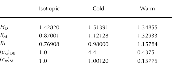
rz, the viscosity factor arising in the ![]() relation (56), and defined by (57). We now present comparisons of the isotropic-ice, cold-ice, and warm-ice solutions for the three bed topographies. Tables 1–3 show H
D, R
M, R
E, (crz
)DB and (crz
)M, where R
E is the scaled radius where Q(H) is zero, and (crz
)DB denotes the value at the base of the divide, here R = 0, Z = 0, given by the asymptotic limit (97), for the flat, hump and basin beds. At the base of the divide, where the vertical compression is large, (crz)DB has the same limit values for all three topographies, but this greatly exceeds unity for cold ice, and is significantly less than unity for warm ice, associated with the limit compression factor A, given in (20), exceeding unity for cold ice and less than unity for warm ice. The viscosity factor at the margin, (crz
)M, decreases from its unit isotropic value for the cold ice, and more dramatically for the warm ice, in the flat- and hump-bed cases, but in the basin-bed case it still decreases dramatically for warm ice, but is close to unity for cold ice. For all three bed forms, the margin span RM
increases from isotropic to cold to warm ice, while the divide height HD
increases slightly then decreases more for the same sequence, but, as expected, increases from basin to flat to hump beds.
relation (56), and defined by (57). We now present comparisons of the isotropic-ice, cold-ice, and warm-ice solutions for the three bed topographies. Tables 1–3 show H
D, R
M, R
E, (crz
)DB and (crz
)M, where R
E is the scaled radius where Q(H) is zero, and (crz
)DB denotes the value at the base of the divide, here R = 0, Z = 0, given by the asymptotic limit (97), for the flat, hump and basin beds. At the base of the divide, where the vertical compression is large, (crz)DB has the same limit values for all three topographies, but this greatly exceeds unity for cold ice, and is significantly less than unity for warm ice, associated with the limit compression factor A, given in (20), exceeding unity for cold ice and less than unity for warm ice. The viscosity factor at the margin, (crz
)M, decreases from its unit isotropic value for the cold ice, and more dramatically for the warm ice, in the flat- and hump-bed cases, but in the basin-bed case it still decreases dramatically for warm ice, but is close to unity for cold ice. For all three bed forms, the margin span RM
increases from isotropic to cold to warm ice, while the divide height HD
increases slightly then decreases more for the same sequence, but, as expected, increases from basin to flat to hump beds.
Table 1. Flat-bed parameters

Table 2. Hump-bed parameters

Table 3. Basin-bed parameters
Figures 3–5 show the bed and surface profiles for the isotropic, cold and warm ice, for the flat, hump and basin beds, respectively. These illustrate the distinct, and significant, effects of the two forms of fabric evolution treated, particularly on the span R M. For a given R M and fabric law, the divide height H D is essentially governed by the steady-state assumption, that there is no net flux in or out of the sheet.

Fig. 3. Free surface profiles for isotropic, cold and warm ice; for flat bed.

Fig. 4. Free surface profiles for isotropic, cold and warm ice on the illustrated basin bed. illustrated hump bed.

Fig. 5. Free surface profiles for isotropic, cold and warm ice on the illustrated basin bed.
The viscosity factor crz is identically unity for the isotropic ice. Figure 6 shows the distribution of crz , first down the divide as a function of H – Z, then along the bed as a function of R, for cold and warm ice, in the flat-bed case. This gives a measure of how the fabric is affecting the shearing rate of the ice, down the symmetry axis and along the bed. Figure 7 shows the same for the hump bed and Figure 8 for the basin bed. There is a significant effect from the bed topographies. While crz for the warm ice is mainly decreasing along these two boundaries, consistent with the increase of span R M from the isotropic span, the effect of decreasing crz along the bed, and in the sheet interior, for the cold ice, must offset the increase down the divide, since R M is again greater than the isotropic span for each bed form, though less than the warm span.

Fig. 6. Distributions of the viscosity factor, crz , down the divide (as a function of H – Z) and along the bed (as a function of R) for cold and warm ice; for flat bed.

Fig. 7. Distributions of the viscosity factor, crz , down the divide (as a function of H — Z) and along the bed (as a function of R) for cold and warm ice; for flat bed.

Fig. 8. Distributions of the viscosity factor, crz , down the divide (as a function of H — Z) and along the bed (as a function of R) for cold and warm ice; for basin bed.
Figure 9 shows, for the flat bed, the distributions of the horizontal scaled velocity, U, with height at locations R = 0.2, R = 0.4, R = 0.6 for isotropic, cold and warm ice. Recall that the hump/basin topographies are centred at R c = 0.4. The effects of fabric are increased with distance from the divide as expected, particularly near the bed. Figure 10 shows the same for the hump bed, and Figure 11 for the basin bed, with similar effects, and with increased changes near the bed due to the topographies.

Fig. 9. Horizontal velocity depth profiles at R = 0.2, R = 0.4 and R = 0.6, for isotropic, cold and warm ice; for flat bed.

Fig. 10. Horizontal velocity depth profiles at R = 0.2, R = 0.4 and R = 0.6, for isotropic, cold and warm ice; for hump bed.

Fig. 11. Horizontal velocity depth profiles at R = 0.2, R = 0.4 and R = 0.6, for isotropic, cold and warm ice; for basin bed.
9. Conclusions
An enhanced reduced model for steady radially symmetric flow of an ice sheet with fabric evolution, over bed topographies with a modest maximum slope, S, has been derived, where є ≪ δ ≪ 1 and є is the surface slope magnitude. It is described by the leading order balances of the mass and momentum equations, boundary conditions and the constitutive law for the ice governing the fabric (induced anisotropy) evolution, with errors of order δ.
Numerical solutions for a flat bed, a bed with a single symmetric hump and a bed with a single symmetric basin have been constructed, for two forms of the fabric evolution, described as cold ice and warm ice. Tables of the key parameters – divide height, margin radius, equilibrium-line radius and the fabric-induced viscosity factor – are presented for the isotropic, cold and warm ice for each of the bed forms. The radial span, margin radius, is seen to be strongly influenced by the induced fabric. Figures illustrate the distinct ice-sheet profiles, the distribution of the fabric- induced viscosity factor down the divide and along the bed, and the distributions with height of the horizontal velocity, for the different ice laws and bed topographies. All illustrate the significant effect of fabric evolution compared to the conventional isotropic ice model.
The adopted fabric-evolution model does not account for possible fabric weakening due to migration recrystallization occurring at high (near-melting) temperature or high strain rate, which may arise in thin zones near an ice-sheet bed. Since bed conditions have a major influence on the flow and profile, such weakening could make a significant difference to the solutions and conclusions. If, however, such zones are not extensive, but confined to limited areas of the bed, then the magnitudes of the effects derived here may still apply. To reach a firmer conclusion, a constitutive model which realistically describes such weakening effects must first be established and incorporated in the ice-sheet flow equations, and then solutions for simple flow configurations obtained.
Acknowledgement
The theoretical development was completed during a UK Engineering and Physical Sciences Research Council project, ‘Evolving Anisotropy in Ice Sheet Flows’.


