


1. Introduction
Secondary flows occurring in nature and in many engineering applications have attracted significant attention due to their impact on the flow structure, as well as the complex underlying physical mechanisms producing them. Secondary flows can be categorized into two types: (i) the first kind, where their generation is primarily an inviscid process, and examples can be found in both laminar and turbulent flows (i.e. flow through curved pipes); (ii) the second kind, where the generation mechanism is attributed to Reynolds stresses second gradients and therefore can be only found in turbulent flows (i.e. flows through square ducts). Further details and analysis of this classification can be found in the review paper by Bradshaw (Reference Bradshaw1987). As of today, most of the research in this field has been focused on of secondary flows of the second kind that occur in non-circular ducts (see for example Pirozzoli et al. Reference Pirozzoli, Modesti, Orlandi and Grasso2018; Nikitin, Popelenskaya & Stroh Reference Nikitin, Popelenskaya and Stroh2021), and other corner flows (i.e. Grega et al. Reference Grega, Wei, Leighton and Neves1995; Nasiri & Balaras Reference Nasiri and Balaras2020). Recent research also points to the generation of secondary flows in turbulent boundary layers evolving over various rough walls. These are mean flow features that exist in the cross-stream plane perpendicular to the dominant flow direction (see for example Anderson et al. Reference Anderson, Barros, Christensen and Awasthi2015). Today, our understanding of how these secondary motions are produced and correlate to the roughness topography, or how they impact the flow statistics and similarity laws, is far from complete.
In rough-wall boundary layers, early observations of secondary flows were directly linked to topographies with regular arrangements of roughness elements. Reynolds et al. (Reference Reynolds, Hayden, Castro and Robins2007), for example, conducted an experimental study of turbulent boundary layers developing over staggered cube arrangements and reported significant, streamwise persistent, periodic variations of the mean streamwise velocity in the spanwise direction, which were attributed to the particular topographical pattern. Vanderwel & Ganapathisubramani (Reference Vanderwel and Ganapathisubramani2015) investigated turbulent boundary layer flows over strips of roughness oriented in the streamwise direction and detected spanwise-periodic variations in the mean streamwise velocity, which also seemed to be correlated to the periodicity of the topographical pattern. They also found that, in order for secondary motions to be formed, the spacing,  $S$, between roughness elements has to be rather coarse: $S/\delta \geq 0.5$ (where $\delta$ is the local boundary layer thickness). In a recent experimental study, Womack et al. (Reference Womack, Volino, Meneveau and Schultz2022) considered the evolution of a turbulent boundary layer over staggered and random arrangements of truncated cones at various coverage levels. Contrary to the above studies they observed secondary flows for the case of the random arrangements but not for the staggered ones. Mejia-Alvarez & Christensen (Reference Mejia-Alvarez and Christensen2013) reported experiments in a zero pressure gradient turbulent boundary layer evolving over highly irregular roughness and also showed evidence of secondary flows, which were manifested as regions with mean streamwise momentum deficit or low momentum pathways (LMP), and regions with mean streamwise momentum surplus or high momentum pathways (HMP). The formation of such momentum pathways was attributed to a possible channelling of the flow induced by the irregular roughness. They also suggested that LMP and HMP show a spanwise-alternating presence. In a followup study Barros & Christensen (Reference Barros and Christensen2014) suggested that the LMP are primarily correlated with recessed local topography, and the HMP with elevated local topography. They also noted that the spanwise locations of enhanced turbulent kinetic energy (TKE) and Reynolds stresses coincide with those of the LMP. However, Womack et al. (Reference Womack, Volino, Meneveau and Schultz2022), who also identified HMP and LMP over randomly arranged truncated cones, found no correlation between the spanwise locations of the momentum pathways and the local topography, but instead they noted that a correlation may exist with the leading part of the roughness.
Although secondary flows are only a small percentage of the mean streamwise velocity they are known to affect the overall flow structure, and may have an impact on similarity laws that are typically utilized to scale experimental and computational results to field scale Reynolds numbers. Outer-layer similarity (Townsend Reference Townsend1976), for example, is commonly utilized in turbulent boundary layer flows over rough walls although universal criteria defining its applicability limits have not yet been fully established. Jiménez (Reference Jiménez2004) suggested a blockage ratio  $\delta /k \geq 40$, where k is the characteristic height of the roughness, for Townsend's wall similarity hypothesis to be valid. Flack, Schultz & Shapiro (Reference Flack, Schultz and Shapiro2005), on the other hand, suggested to use the ratio of the boundary layer thickness to the equivalent sand-grain roughness height ( $\delta /k{_s}$) with a limit at $\delta /k{_s} \geq 40$. The latter is also supported by the findings of Wu & Christensen (Reference Wu and Christensen2007). Yang & Anderson (Reference Yang and Anderson2017) by performing large-eddy simulations (LES) over streamwise-aligned rows of pyramidal roughness elements proposed that the spanwise spacing, $s_z$, between adjacent patches of high and low roughness could act as a prognostic parameter to assess the possible distortion of the outer-layer similarity due to secondary motions. Womack et al. (Reference Womack, Volino, Meneveau and Schultz2022) noted that the lack of well-established criteria highlights a lack of understanding of the correlation between the physical mechanisms present in rough-wall flows and the surface statistics. They further demonstrated a breakdown of the outer-layer similarity for the flows over the random topographical arrangements and attributed it to the presence of strong secondary flows. Similar breakdown of the outer-layer similarity and conclusions were reported in Medjnoun, Vanderwel & Ganapathisubramani (Reference Medjnoun, Vanderwel and Ganapathisubramani2018), where experiments were conducted for a turbulent boundary layer over streamwise-aligned roughness strips.
The present work focuses on the origin and evolution of secondary flows in turbulent boundary layers with zero pressure gradients developing over truncated cones in staggered and random arrangements. In particular, direct numerical simulation (DNS) will be presented, where the roughness geometries and parametric space closely matches the experiments reported by Womack et al. (Reference Womack, Volino, Meneveau and Schultz2022). After validating our computations by direct comparison with the experiments, our primary objectives are to investigate: (i) the relation of the secondary flows to the topographical features for regular and random surfaces as there has been conflicting evidence in the literature; (ii) the impact of secondary flows on the flow structure and scaling laws. In the § 2 we describe the numerical methods and techniques implemented to address the physical problem and the topographies studied. In § 3 we demonstrate agreement in the first- and second-order statistics with the experimental measurements of Womack et al. (Reference Womack, Volino, Meneveau and Schultz2022) for all the topographies considered. In § 4 we discuss the main observations of the momentum pathways between the various topographies and present their correlation with the topographical statistics, while in § 5 we comment on the nature of the secondary flows observed by conducting a vorticity transport analysis.
2. Methodologies and parametric space
Following Womack et al. (Reference Womack, Volino, Meneveau and Schultz2022), the rough surface was created utilizing truncated cones (see figure 1c) in random and staggered configurations, which resemble barnacles found on fouled ship hulls. For the staggered arrangement, a coverage level of 39 % (S39) is considered, while for the random we will report three coverage levels: 10 % (R10), 17 % (R17) and 39 % (R39). A top view of each arrangement is shown in figure 2. In the experimental study a boundary layer with zero pressure gradient develops over a smooth surface upstream of the roughness patch. The trip wire producing the turbulent boundary layer was positioned  $0.78$ m upstream of the roughness leading edge while the measurement station was approximately $0.75$ m downstream. The computational domain matches exactly the dimensions of the roughness patch utilized in the experiments. To reduce the computational cost a truncated smooth part was added upstream and downstream to facilitate implementation of appropriate boundary conditions. The resulting domain is shown in figure 1(b), and extends $200D \times 28D$, in the streamwise $(x)$ and spanwise $(z)$ directions respectively ( $D$ is the base diameter of the truncated cone). The free-stream boundary is positioned at $20D$ from the wall. At the inflow plane, velocity boundary conditions are extracted from a precursor simulation (see figure 1a,b) that was designed to match the Reynolds number in the experiments at $30D$ upstream of the leading edge of the roughness. In particular, we set ${Re_\theta }^{(inflow)}=U_e \theta _o/\nu = 1600$ (where $\theta _o$ is the momentum thickness at the inflow plane, $U_e$ the free-stream velocity and $\nu$ the kinematic viscosity), corresponding to ${Re_\tau }^{(inflow)} = u_\tau \delta _o/\nu = 550$ (where $\delta _o$ is the boundary layer thickness at the inflow plane and $u_\tau$ the friction velocity at the inflow plane). The boundary layer thickness compared with the roughness elements is set equal to $\delta _o/D=1.3$. The corresponding Reynolds numbers at the leading edge of the roughness in the case of a smooth wall are equal to ${Re_\tau }^{(LE)} = 750$ and ${Re_\theta }^{(LE)} = 2100$. A convective boundary condition was used at the outflow plane and radiative conditions at the free-stream boundary (see Piomelli, Balaras & Pascarelli Reference Piomelli, Balaras and Pascarelli2000, for details).

Figure 1. Computational set-up corresponding to the experiments reported by Womack et al. (Reference Womack, Volino, Meneveau and Schultz2022). (a) Precursor simulation to generate inflow boundary conditions. (b) Computational domain used for all production runs. (c) Truncated cones used to generated all topographies.

Figure 2. Top view of the different topographies considered: (a) staggered S39; (b) random R39; (c) the random, R17; (d) the random, R10.
The Navier–Stokes equations for incompressible flow are solved on a structured Cartesian grid using an in-house finite-difference solver coupled to an immersed-boundary formulation. For the time advancement a semi-explicit method is employed, where all terms are treated explicitly using the Runge–Kutta third-order scheme, except for the viscous and convective terms in the wall-normal direction which are treated implicitly using a second-order Crank–Nicholson scheme. All spatial derivatives are discretized using second-order central differences on a staggered grid. The code is parallelized using a classical domain decomposition approach. The roughness elements were immersed in a Cartesian grid and the no-slip condition was enforced using an immersed-boundary (IB) formulation. The details on the overall formulation can be found in Yang & Balaras (Reference Yang and Balaras2006). The computational grid was designed to be approximately uniform in the area covered by the roughness elements, where the resolution is the highest. The grid spacing was gradually increased moving away from the roughness area in a way that the resolution is appropriate for a turbulent boundary layer over a smooth plate for this range of Reynolds numbers. In all production runs a grid utilizing  $6002 \times 1202 \times 348$ points in the streamwise $(x)$, spanwise $(z)$ and wall-normal $(y)$ directions, respectively, was used. This results in $\Delta x^+=10.5$, $\Delta z^+=9$ and $0.9 \leq \Delta y^+ \leq 20$ (based on the friction velocity, $u_\tau$, on the smooth part of the plate). The corresponding number of nodes around individual roughness elements (i.e. a volume of size $D\times D \times 0.45D$ in $x,z,y$, respectively) is approximately $40\times 40 \times 70$. We adopted the above resolution after a grid refinement study involving a coarser and a finer (by a factor of 2) grid in a reduced domain. The details together with comparisons of the statistics are given in Appendix A.
3. Streamwise flow evolution and validation
In this section we will examine the impact of the topography on the evolution of the boundary layer and compare the statistics of the velocity field at the measurement station ( $x/D=133$) with the corresponding ones reported in Womack et al. (Reference Womack, Volino, Meneveau and Schultz2022). The four topographies under consideration are shown in figure 2. The evolution of the boundary layer thickness, $\delta /D$, momentum thickness, $\theta /D$, and friction velocity, $u_\tau /U_e$, is shown in figure 3. The evolution is similar for the S39 and R39 cases, indicating that the coverage level affects the growth of the boundary layers more than the type of arrangement (staggered or random). As the coverage decreases both $\delta /D$ and $\theta /D$ grow slower and at the measurement station, $x/D=133$, the difference in the boundary layer thickness between the R39 and R17 cases is approximately $11\,\%$.

Figure 3. Streamwise evolution of: (a) boundary layer thickness,  $\delta /D$; (b) momentum thickness, $\theta /D$. Red solid line, S39; blue dashed line, R39; green dashed-dotted line, R17; orange dotted line, R10. Black solid line indicates the roughness leading edge; dashed-dotted-dotted line indicates the measurement location in the experiments by Womack et al. (Reference Womack, Volino, Meneveau and Schultz2022).
Accurate prediction of the drag coefficient is crucial for the naval engineering applications involving biofouled surfaces, since drag is linked to the fuel consumption of the naval vessel. The significance of the latter is underlined and quantitatively explained in Schultz et al. (Reference Schultz, Bendick, Holm and Hertel2011). In DNS over rough-wall boundary layers using IB methods the computation of a representative friction velocity,  $u_\tau (x)/U_e$, at a streamwise location, $x$, is a non-trivial task. This is due to: (i) direct computation of $u_\tau /U_e$ on the rough surface requiring the mean flow variables (velocity derivatives and pressure) on the boundary, which are not directly defined. In recent computations reported in the literature this issue is bypassed by utilizing momentum balance (MB) approaches, where the total force acting on a local area is inferred from the MB over a properly defined volume (i.e. Yuan & Piomelli Reference Yuan and Piomelli2014). This results in fairly accurate computation of the total forces but one cannot decompose them into pressure and viscous contributions in a straightforward manner. In this work, we utilize a formulation which is based on the direct integration of the viscous and pressure contributions on local elements and, as a result, viscous and pressure parts can be identified. The details are given in Appendix B. (ii) Due to cost considerations the computational domain in the spanwise direction, where periodic conditions are utilized, is limited while time averaging can only be performed over a fraction of the eddy turnover times used in the experiments. As a result, direct spanwise averaging at a streamwise location, $x$, of the surface values of $u_\tau /U_e$, only involves a limited number of barnacles. This results in a fairly noisy evolution of $u_\tau (x)/U_e$. We found that this is mainly due to the presence of strong pressure outliers coming from local topographical singularities (e.g. roughness clusters), which are not averaged out due the limited number of barnacles involved in the computation of $u_\tau (x)/U_e$. To increase the latter we performed additional averaging over the surface elements contained in a narrow spanwise strip around the streamwise location, $x$. This strategy increases the number of roughness elements involved in the computation of the wall stress and results in a smoother streamwise evolution. For the results presented below the streamwise extent of the spanwise strip was between $4D$ and $8D$, depending on the topography. The details of the method together with a sensitivity analysis on the extent of the averaging strip in the spanwise direction is given in Appendix B. The resulting distribution of $u_\tau (x)/U_e$ for the four cases considered is shown in figure 4(a). For all cases the transition from a smooth to a rough wall is characterized by an increase in the friction velocity that quickly reduces to the rough-wall value over approximately $50D$. In the case of the staggered arrangement, S39, the peak is three times higher than in all random cases probably due to the uniformly distributed, high solidity in the area. After this initial adjustment the wall stress for all cases gradually decreases with the same slope as the boundary layer thickens.

Figure 4. (a) Streamwise evolution of the friction velocity,  $u_\tau /U_e$: red solid line, S39; blue dashed line, R39; green dashed-dotted line, R17; orange dotted line, R10. Black solid line indicates the roughness leading edge; dashed-dotted-dotted line indicates the measurement location in the experiments by Womack et al. (Reference Womack, Volino, Meneveau and Schultz2022). Time- and spanwise-averaged streamwise velocity profiles in inner coordinates for (b) S39 and (c) R39; red solid line, $x/D=80$; green solid line, $x/D=100$; blue solid line, $x/D=120$; black solid line, $x/D=140$. black dashed line represents the log law with $\kappa =0.384$ and $\beta =4.2$.
Direct comparisons of the predicted friction velocity with the corresponding values reported in the experiments by Womack et al. (Reference Womack, Volino, Meneveau and Schultz2022) are given in table 1. All listed values are at the experimental measurement location  $x/D=103$ from the leading edge of the roughness. Overall the agreement with the experiment is excellent (within 2 %) with the exception of the R39 case where the friction velocity is under-predicted by approximately 7 %. This may be due to the limited time-averaging sample in the DNS. The breakdown of the friction velocity into pressure and viscous contributions obtained from the DNS are also listed in the last two columns in the table. The pressure contribution overtakes the viscous one in every topography, which can be attributed to the low ratios of the boundary layer thickness compared with the roughness height, $\delta /k$. As expected, the pressure contribution decreases as the percentage coverage decreases, which is also pointed out in Schultz (Reference Schultz2004). Specifically, in the R39 arrangement the pressure and viscous contributions to the friction velocity are approximately 87 % and 13 %, respectively, whereas at the lower coverage R10 they are 67 % and 33 %. The ratio between the pressure and viscous contributions persists in the streamwise direction for all the topographical arrangements. The predicted friction velocity also collapses well the mean streamwise velocities profiles in inner coordinates at various streamwise locations over the equilibrium rough part of the plate (figure 4b).
Table 1. Friction velocity ( ${u_\tau }/{U_e}$) with respect to the different topographical cases as reported by the experimental work of Womack et al. (Reference Womack, Volino, Meneveau and Schultz2022) together with the friction velocity computed by the current DNS study at the experimental measurement location. The individual contribution of pressure and viscous forces computed by the current DNS study is also included.

To further establish the accuracy of the DNS we directly compare the mean velocity profiles and normal Reynolds stresses at the measurement station. To eliminate uncertainties coming from the estimation of the friction velocity in the experiment and simulations, outer coordinates are used (see figure 5). Overall, the agreement is very good and it is within the experimental uncertainty and sampling error in the DNS. We have selected two cases with the highest (R39) and lowest (R10) coverage but the same trends were observed for all cases we computed.

Figure 5. Mean velocity and normal Reynolds stresses profiles at the experimental measurement location ( $x/D=133$). (a) Mean velocity R39; (b) mean velocity R10; (c) normal stresses R39; (d) normal stresses R10. Lines are from the DNS and symbols from the corresponding experimental results by Womack et al. (Reference Womack, Volino, Meneveau and Schultz2022). Red solid line, $\bar{u}/U_e$; red dashed line, $\overline {u'u'}/{U_e}^2$; red dashed-dotted line, $\overline {v'v'}/{U_e}^2$.
4. Secondary flow patterns
Secondary flows in the cross-stream plane of a turbulent boundary layer have a direct impact on the mean streamwise velocity. This is manifested as bending of the isolines of the streamwise velocity at the ( $y$–
$y$– $z$) plane, which will otherwise be parallel to the wall. An example is shown in figure 6 where isolines of the mean streamwise velocity at a plane located at $x/D=133$ for the random R39 case, are compared with the corresponding data from the experimental study by Womack et al. (Reference Womack, Volino, Meneveau and Schultz2022). The agreement is very good and the DNS captures the structure of the secondary flows very accurately. Looking at the velocity variation at a line parallel to the wall, it is clear that regions of high and low velocity fluid are created. Those pathways were first observed/defined by Mejia-Alvarez & Christensen (Reference Mejia-Alvarez and Christensen2013) and are usually referred too as HMP and LMP. These are also alternating in the spanwise direction, as indicated by the solid and dashed lines in figure 6. We should note that persistent spanwise inhomogeneities in the mean streamwise velocity have also been reported (see for example Fishpool, Lardeau & Leschziner Reference Fishpool, Lardeau and Leschziner2009), as a result of an insufficient temporal sample. The agreement between the simulations and the experiments in figure 6 indicates that the spanwise inhomogeneity is not due to the lack of sample size given that the experiment utilizes more than $10\,000$ eddy turnover times, $\delta /U_e$. To reinforce that the agreement is not a fortuitous coincidence we increased the sample for the R39 case and compared the results for $50\delta /U_e$, $100 \delta /U_e$ and 200 $\delta /U_e$. All sampling windows produce the same streamwise mean flow within 2 %. Details are given in Appendix A.

Figure 6. Isolines of the time-averaged streamwise velocity  $\bar{u}/U_e$ in a cross-stream plane at the experimental measurement location ( $x/D=133$). Random, R39 topography. (a) Womack et al. (Reference Womack, Volino, Meneveau and Schultz2022); (b) DNS. Solid lines represent the HMP and dashed lines the LMP.
It is worth noting that, in agreement with the observations by Womack et al. (Reference Womack, Volino, Meneveau and Schultz2022), the present results indicate a breakdown in the outer-layer similarity for the mean streamwise velocity, particularly for the random arrangements, due to the presence of the secondary flows. The mean velocity profiles in outer coordinates for S39 and R39 are shown in figure 7. All profiles are extracted at the same streamwise location ( $x/D=133$) at different spanwise stations. The velocity profiles in the staggered arrangement show good overall convergence (less than $10\,\%$ difference across the boundary layer). For the random topography, on the other hand, a significant difference across the whole boundary layer can be seen. The largest difference occurs in the R39 arrangement where the maximum deviation at a height of $2k$ is around $30\,\%$, but the trends are the same for all random arrangements (not shown here). Neither of the two cases (S39 and R39) meets the criteria for outer-layer similarity suggested by Jiménez (Reference Jiménez2004) ( $\delta /k \geq 40$) and Flack et al. (Reference Flack, Schultz and Shapiro2005) ( $\delta /k_s \geq 40$) as both ratios are less than fifteen. The striking difference between the random and staggered configurations, however, indicates that the outer-layer similarity not only depends on the blockage ratios, $\delta /k$ and $\delta /k_s$, which are very similar between topographies with same percentage coverages, but also on the topographical characteristics of the particular rough surface. The latter observation regarding the $\delta /k$ it is also pointed out in the recent review of Chung et al. (Reference Chung, Hutchins, Schultz and Flack2021).

Figure 7. Mean streamwise velocity vs wall-normal distance in outer coordinates at the experimental measurement location ( $x/D=133$) for various spanwise coordinates (black solid line, spanwise-averaged velocity profile) for the: (a) staggered S39 topography; (b) random R39 topography.
The three-dimensional evolution of HMP and LMP can be captured by defining a mean streamwise velocity where the spanwise average at each  $x$ location is removed, similar to Wangsawijaya et al. (Reference Wangsawijaya, Baidya, Chung, Marusic and Hutchins2020): $\tilde {u}/U_e = \bar {u}/U_e - \langle \bar {u}/U_e \rangle _z$, where $\bar {.}$ is the time-averaging operator and $\langle.\rangle _z$ is the spanwise-averaging operator. Areas where $\tilde {u}/U_e>0$ capture the HMP, and areas where $\tilde {u}/U_e<0$ capture LMP. A top view visualization of HMP/LMP captured by isosurfaces of $\tilde {u}$ is shown in figure 8 for all the topographies considered in this study. A direct comparison of HMP/LMP for the staggered and random arrangements for the same coverage of 39 % (figure 8a,b) reveals a striking difference: momentum pathways generated over the staggered arrangement follow the topographical pattern throughout the roughness region and are very repeatable; LMPs are formed in the windward area of each roughness element, and the HMPs in the regions between (this is better illustrated in figure 9a). For the random arrangement, on the other hand, pathways are formed immediately after the leading edge of the roughness and persist even past the end of the roughness area, showing a striking degree of streamwise coherence. This trend is evident for all coverage levels as seen in figure 8(c,d). This finding indicates a far bigger streamwise persistence of the momentum pathways compared with what previous studies had reported (see for example Mejia-Alvarez & Christensen Reference Mejia-Alvarez and Christensen2013). This streamwise persistence is also an indication that HMP and LMP over the random topographies are not directly correlated with the local topography, as for the case of staggered arrangements.

Figure 8. Top view of isosurfaces of  $\tilde {u}/U_e$. The HMP are shown in red solid line ( $\tilde {u}/U_e= 5\,\%$); LMP are shown in blue solid line ( $\tilde {u}/U_e = -5\,\%$): (a) staggered, S39 topography; (b) random, R39 topography; (c) random, R17 topography; (d) random, R10 topography.

Figure 9. Isolines of  $\tilde {u}/U_e$ capturing the momentum pathways at the three streamwise locations indicated with green lines in figure 8(a,b). Panels (a,c,e) staggered S39 topography; (b,d,f) random, R39 topography; (a,b) $x/D=30$; (c,d) $x/D=80$; (e,f) $x/D=133$. The solid line represents the boundary layer edge. The bold and light dashed lines represent the topography at the current and at a $1D$ further downstream topography, respectively.
To better illustrate the streamwise evolution of the pathways and their location within the boundary layer figure 9 shows isolines of  $\tilde {u}/U_e$ in the cross-stream plane at three different streamwise locations, $x/D=30$, $x/D=80$ and $x/D=133$ (indicated in figure 8a,b) for the staggered and random topographies at 39 % coverage. The edge of the boundary layer is also indicated with a solid black line. Clearly the momentum pathways for the staggered case (figure 9a,c,e) are weak and confined to the roughness crest throughout the rough region. This may also be the reason that no such pathways were detected in the experiments by Womack et al. (Reference Womack, Volino, Meneveau and Schultz2022), as their first measurement point off the wall was typically above the top of the roughness elements. It is interesting to note that Vanderwel & Ganapathisubramani (Reference Vanderwel and Ganapathisubramani2015) examined the impact of the spanwise spacing, $S$, on the formation of secondary flows for canonical topographies consisting of streamwise oriented strips, and suggested $S/\delta > 0.5$ is a necessary condition for the secondary motions to be detectable above the roughness sublayer. For the case of S39 this ratio always remains below the threshold. For the random arrangement, on the other hand, the momentum pathways are located higher in the boundary layer even at the leading edge region and more evidently further downstream when they almost reach the boundary layer edge (see figure 9b,d,f). The impact of the larger wall-normal location of the momentum pathways formed over the R39 arrangement compared with those over the S39 can be also indirectly seen in figure 9(b) via the significant distortion of the boundary layer edge.
The above analysis and the profound differences between the staggered and the random topographies give rise to questions such as how are secondary flows generated, and what is their relation to the topography? It is clear that the momentum pathways over the staggered arrangement are highly influenced by the local topography. In particular, LMP and HMP in the staggered arrangement seem to be correlated with the increased and decreased local topography, respectively. There is no indication of such correlation for the random topographies, where the leading edge of the roughness appears to be better correlated with their origin. The latter was also conjectured in the experimental study by Womack et al. (Reference Womack, Volino, Meneveau and Schultz2022). To quantify such correlations we employ a sample volume technique (SVT), where consecutive volumes in the spanwise direction are generated at a specific streamwise station. To capture a representative sample of the surface we define volumes that cover the rough surface and have a streamwise and spanwise length of  $\sim 3\bar {d}_{min}$ (where $\bar {d}_{min}$ is mean minimum distance to neighbouring roughness elements), and varying height (i.e. 2 to 20 times the roughness height, $k$) depending on their streamwise location in order to overlap with the HMP/LMP in the boundary layer. In each volume an average value of the local surface statistics is computed (e.g. frontal area, effective slope, mean height etc.) together with the average of $\tilde {u}/U_e$, which indicates the presence of HMP/LMP. Figure 10 shows the correlation between the frontal area, $\lambda _f$, and the momentum pathways using the SVT technique for the cases of S39 and R39. At the leading edge of the roughness there is a clear correlation between LMP and increased frontal area as well as between HMP and decreased frontal area for both topographies (see figure 10a,b). Similar trends (not shown here) were observed for the rest of the topographies, as well as for other topographical statistics such as the effective slope ( $ES$) and the mean roughness height ( $\bar {k}$). This correlation remains strong at the downstream station ( $x/D=133$) for the case of the staggered topography, while no correlation is observed for the random case (see figure 10c,d). This trend is further reinforced by looking at correlation of the same quantities, but computed this time over the full extent of the roughness area (see figure 11). For the staggered arrangement the correlation of LMP with elevated topography and HMP with recessed topography is consistent. For the random arrangement on the other hand, no such trend can be observed and the HMP/LMP are evenly distributed over the full range of $\lambda _f$. These trends were also very similar for the cases of R17 and R10. Additionally, it should be noted that the random topographies generate stronger momentum pathways (figure 10b) due to locally significant element clustering (i.e. frontal solidity accumulation) present at the leading edge.

Figure 10. The relation between the momentum pathways and topography at two streamwise locations visualized by the correlation between frontal area coverage,  $\lambda _f$, indicated by black solid line and momentum pathways indicated by $\bullet$, red for HMP and $\bullet$, blue for LMP computed using the SVT approach: (a) S39 at $x/D=30$; (b) R39 at $x/D=30$; (c) S39 at $x/D=133$; (d) R39 at $x/D=133$.

Figure 11. Momentum pathways ( $\bullet$, red for HMP and $\bullet$, blue for LMP) vs frontal area coverage, $\lambda _f$, as computed using the SVT approach over the whole extent of the rough area: (a) staggered S39 topography; (b) random R39 topography.
The above results point to a direct correlation of the leading edge topography to the resulting secondary flow patterns for all random arrangements. To further investigate this correlation we conducted a series of numerical experiments using the random arrangement, R39, as a baseline test case. We introduced the following modifications at the leading edge:
(i) The leading edge roughness is altered by decreasing the height of the clustered roughness elements that correlate with the momentum pathways, and increasing the height of the isolated ones, keeping the spatial coordinates and planar solidity the same. The modified topography can be seen in figure 12(b), where the elevated and recessed roughness elements are colour coded. A comparison of the momentum pathways at the leading edge between the original and the modified configuration (figure 12d–e) shows that the regions in the original R39 arrangement that were occupied by elevated clusters and LMP are now regions with recessed clusters and HMP. This is further reinforced in figure 12(g–h), where the correlation between momentum pathways and local topography is illustrated via the SVT approach. It is clear that the formation of the momentum pathways does not occur at fixed spanwise locations but instead is subject to the specific distribution of the leading edge topography. Although both the new HMP/LMP now reside in different spanwise locations, they still expand further downstream and again depart from the wall. Therefore, that means that one can alter the form and strength of the secondary flows found over multiple boundary layer thicknesses downstream by just alternating the leading edge roughness.

Figure 12. Random R39 topography in (a) baseline; (b) modified leading edge; (c) only leading edge roughness configurations; (d,e, f) corresponding isosurfaces of  $\tilde {u}/U_e$, red solid line HMP and blue solid line LMP; (g,h) corresponding correlation of $\tilde {u}/U_e$ to frontal area coverage, $\lambda _f$ at the leading edge of the roughness; ( $\bullet$, red HMP; $\bullet$, blue LMP); (i) correlation of $\tilde {u}/U_e$ between the original R39 configuration (solid circles) and the leading edge roughness only configuration (hollow circles) for half of the computational domain in the spanwise direction at the experimental measurement location ( $x/D=133$) using the SVT.
(ii) Only the leading edge roughness is maintained in which the original height and spatial coordinates are kept the same as in the original arrangement, while the rest of the rough domain is replaced by a smooth wall (see figure 12c). The aim of this numerical experiment is to investigate the strength and streamwise coherence of the momentum pathways formed when only the leading edge topography is considered and how those are compared with the original configuration. Figure 12(f,i) shows that the momentum pathways are still formed at the same locations even in the absence of the downstream topography. Their strength, however, is reduced, probably due to the lower growth rate of the boundary layer over the smooth plate. Upon adjusting the isosurface levels, however, (e.g.  $\tilde {u}/U_e=\pm 2\,\%$) the streamwise coherence of the momentum pathways is still significant and extends through the whole domain.
5. Mean streamwise vorticity transport
To better understand the interaction of the secondary flows with the boundary layer developing over the roughness patch, the mean velocity vectors normalized by magnitude are shown at a cross-stream plane in figure 13 at the three streamwise locations indicated in figure 8 ( $x/D=30$, $x/D=80$ and $x/D=133$) for the staggered and random arrangements with 39 % coverage. Contours of
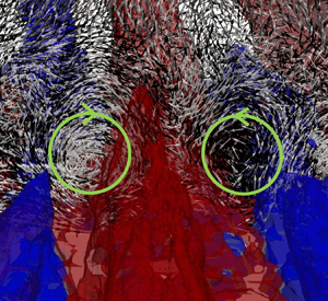
  $\tilde {u}/U_e$ are also included in the background to identify the corresponding momentum pathways. The footprint of the secondary flow patterns is evident in the velocity vectors, but we also added circles indicating their centre and direction of rotation. For the staggered arrangement (figure 13a,c,e) a repeated spanwise pattern develops, where the secondary flows in the form of counter-rotating vortices facilitate lateral momentum exchange which takes place in the area between two consecutive roughness elements. This is confined below the roughness crest for all streamwise locations. The location of HMP/LMP in the background indicates that high momentum fluid is laterally transferred from HMP regions towards LMP, which is consistent with the earlier observations by Womack et al. (Reference Womack, Volino, Meneveau and Schultz2022), Barros & Christensen (Reference Barros and Christensen2014) and Anderson et al. (Reference Anderson, Barros, Christensen and Awasthi2015). The structure of the secondary flows appears to be similar to the one observed in corner flows, where secondary flows of Prandtl's second kind are formed and high momentum fluid is transferred from the core towards the corners (Pirozzoli et al. Reference Pirozzoli, Modesti, Orlandi and Grasso2018). Furthermore, similar counter-rotating motions with significant streamwise coherence have been observed over longitudinal surface roughness in the DNS by Hwang & Lee (Reference Hwang and Lee2018). For the case of the random arrangement (figure 13b,d,f) such vortex pairs are also present but now they can be found throughout the boundary layer. The lateral momentum transfer follows similar behaviour as in the staggered arrangements, where high momentum fluid further away from the wall is transported through the HMP towards the wall. The counter-rotating vortex pairs are located in regions between the HMP and LMP, typically close to the base of the HMP. They are also more coherent when compared with the ones in the staggered arrangement.

Figure 13. Mean velocity vectors normalized by magnitude in a cross-stream plane. Contours of  $\tilde {u}/U_e$ identifying HMP/LMP are shown in the background. Panels (a,c,e) S39; (b,d,f) R39; (a,b) $x/D=30$; (c,d) $x/D=80$; (e,f) $x/D=133$. The centre and direction of rotation of the secondary motions seen in the velocity vectors are indicated by the solid green circles.
To better understand the underlying mechanisms responsible for the generation of such secondary flow patterns over rough surfaces we computed all the significant terms in the mean streamwise vorticity equation,  $\bar {\omega }_x$ (see Bradshaw Reference Bradshaw1987, for details):
 $$\begin{gather} \underbrace{\bar{u} \frac{\partial \overline{\omega_x}}{\partial x} + \bar{v} \frac{\partial \overline{\omega_x}}{\partial y} +\bar{w} \frac{\partial \overline{\omega_x}}{\partial z}}_\text{ADV: Advection} = \underbrace{\overline{\omega_x} \frac{\partial \bar{u}}{\partial x} + \overline{\omega_y} \frac{\partial \bar{u}}{\partial y} +\overline{\omega_z} \frac{\partial \bar{u}}{\partial z}}_\text{VST: Vortex Stretching--Tilting} + \underbrace{\nu \left(\frac{\partial^2 \overline{\omega_x}}{\partial x^2} + \frac{\partial^2 \overline{\omega_x}}{\partial y^2} + \frac{\partial^2 \overline{\omega_x}}{\partial z^2}\right)}_\text{DIFF: Diffusion} \nonumber\\ + \underbrace{\left(\frac{\partial^2}{\partial z^2} - \frac{\partial^2}{\partial y^2}\right)\left(\overline{u'v'}\right) + \frac{\partial^2}{\partial y \, \partial z}\left(\overline{{v'}^2} - \overline{{w'}^2}\right),}_\text{RSG: Reynolds Stress 2nd Gradients} \end{gather}$$
where terms are grouped by their physical meaning indicated underneath. Overall in all cases we found that the dominant terms in the right-hand side of (5.1) are the VST and RSG while DIFF was always smaller throughout the boundary layer. Figure 14 shows contours of the Reynolds stress second gradients (RSG) and vortex stretching–tilting (VST) balance terms for R39 at three streamwise locations:  $x/D=30$, $x/D=80$ and $x/D=133$ as indicated in figure 8. Note that the first location is at the leading edge of the roughness, the second at the middle of the roughness domain and the last at the measurement station of the experiments in Womack et al. (Reference Womack, Volino, Meneveau and Schultz2022). For clarity, only half of the computational domain in the spanwise direction is shown. At the leading edge of the roughness ( $x/D=30$) both RSG and VST terms are of the same order of magnitude and both are confined at the roughness crest. Further downstream, however, the RSG terms expand to larger heights following the boundary layer growth, whereas the VST terms are only significant close to the wall where strong shear layers are formed due to the roughness. It should be noted that no correlation was detected between the RSG or VST terms and the secondary flows. To elaborate more on the relation of those terms, a top view of their magnitude difference normalized by the spatially averaged RSG magnitude, $({\left \| VST \right \|}-{\left \| RSG \right \|})/\langle {\left \| RSG \right \|}\rangle _{xz}$, is shown in figure 15, for both the S39 and R39 topographies. It can be seen that at the leading edge of the roughness at a height of $y=k$ ( $k$: roughness element height) strong VST dominance is observed above the regions with elevated roughness, while clear RSG dominance is observed in the wake of those regions as a result of the vortex breakdown due to increased velocity gradients imposed by the roughness, which is spanwise consistent and true for both the S39 and R39 topographies. Furthermore, the regions of VST dominance correlate with the regions where the LMP are initiated, while regions of ${\left \| VST \right \|}-{\left \| RSG \right \|}$ balance with those of the HMP (figure 15a,b). On the other hand, in the downstream topography the regions of VST dominance become a lot weaker and remain confined near the roughness layer for both the S39 (figure 15c) and R39 (not shown here) topographies, while in higher wall-normal locations, where the HMP/LMP are located in the case of random arrangements, the RSG term clearly dominates. The latter can be seen for the case of the R39 arrangement at a height of $y/k = 6$ in figure 15(d). Additionally, it is noted that no correlation can be detected between the momentum pathways and the regions of RSG dominance downstream of the leading edge roughness in any of the random arrangements studied herein. We should note that earlier work by Anderson et al. (Reference Anderson, Barros, Christensen and Awasthi2015) using both computational and experimental approaches suggests that the secondary flows formed over rough-wall boundary layers are the product of the second gradients of the normal and shear stress anisotropies (RSG), and therefore constitute a realization of Prandtl's second kind. This would imply that the magnitude of the VST terms at the region where the secondary flows are initiated (i.e. the leading edge of the roughness) would be significantly lower than the RSG terms, which is contrary to our observations. This indicates that the particular topography as well as flow conditions, which are different between the two studies, may have an important role in the formation of the secondary flow patterns.

Figure 14. Contours of the RSG (a,c,e) and VST (b,d,f) terms in the mean streamwise vorticity transport equation (5.1) for the R39 case: (a,b)  $x/D=30$; (c,d) $x/D=80$; (e,f) $x/D=133$.

Figure 15. Relative ratio of the  $({\left \| VST \right \|}-{\left \| RSG \right \|})/\langle {\left \| RSG \right \|}\rangle _{xz}$ terms in (5.1). Top view near the leading edge of the roughness at the wall-normal distance $y/k = 1$ for (a) the staggered, S39, topography and (b) the random, R39, topography; top view near the experimental measurement location in Womack et al. (Reference Womack, Volino, Meneveau and Schultz2022) at (c) a wall-normal distance of $y/k = 1$ for the staggered, S39, topography and (d) a wall-normal distance of $y/k = 6$ for the random, R39, topography. The bold and dashed lines represent the local HMP and LMP, respectively.
These observations, together with the results previously presented in this section indicate that: (i) the momentum pathways and hence the secondary flows are initiated at the leading edge of the roughness; (ii) they have a direct relation with the local topography at the leading edge roughness; (iii) downstream of the leading edge the secondary flows do not show any correlation to the local topography; (iv) the VST term dominates the RSG term at the leading edge roughness at the regions of elevated topography (i.e. they are not of Prandtl's second kind as in a typical corner flow, for example); (v) at the leading edge of the roughness regions of VST dominance correlate with those of LMP formation; (vi) downstream of the leading edge no correlation can be stated between either VST or RSG terms and the momentum pathways.
6. Conclusion
Direct numerical simulations over a set of rough topographies with regular and irregular arrangements with three different coverage levels are reported. The results are in very good agreement with the corresponding experiments by Womack et al. (Reference Womack, Volino, Meneveau and Schultz2022). Distortion of the streamwise velocity isolines at a cross-stream plane, conceptualized as flow channelling in the form of mean high and low momentum pathways, indicated the existence of strong secondary flows. The momentum pathways in the case of the staggered arrangements were found to be confined to the roughness crest, whereas in the case of the random arrangements they depart from the wall, reaching the boundary layer edge. Correlation of the momentum pathways to the local topography exists for the case of the staggered arrangement, while in the random arrangements such correlation is only valid at the leading edge roughness. The momentum pathways captured over the random topographies are initiated by the leading edge of the roughness and are completely decoupled from the local topography further downstream. Strong correlation of the momentum pathways to various topographical statistics (e.g. frontal area coverage, effective slope etc.) of the leading edge is observed, indicating that the latter plays an important role on the origin and form of the momentum pathways.
Following the behaviour of the momentum pathways, the secondary flows found on the staggered cases are everywhere located close to the wall and weaker compared with those over the random topographies, which expand to larger heights as the boundary layer grows. Counter-rotating vortices are found to be formed in the regions between the HMP and LMP, close to the base of the HMP, as a result of the lateral momentum transfer (high momentum fluid from larger heights to low momentum fluid closer to the wall). Computing all significant terms in the mean streamwise vorticity transport equation revealed significant dominance of the VST terms at the leading edge of the roughness, indicating that the secondary flows are of Prandtl's first kind, which is not the same as in corner flows. Further downstream no direct correlation was detected between the momentum pathways (or equivalently the secondary flows) and related terms in the mean vorticity transport equation.
Finally, significant deviation was found in the mean streamwise velocity profiles recorded over multiple spanwise coordinates for the same streamwise location, demonstrating the direct impact of the secondary flows to the mean flow statistics. The deviation obtained over the random arrangements is significantly larger compared with the staggered arrangement, which is in agreement with experimental work by Womack et al. (Reference Womack, Volino, Meneveau and Schultz2022).
Declaration of interests
The authors report no conflict of interest.
Appendix A. Effects of grid resolution and sample size
For the topographies and flow conditions selected in the present work the roughness elements occupy a significant portion of the boundary layer, where  $4<\delta / k <12$. This is a form-drag dominated regime and the resolution around these elements is pivotal in capturing the near-wall flow dynamics.
To select the proper resolution we used prior studies in the literature as a guide (see for example Coceal et al. Reference Coceal, Thomas, Castro and Belcher2006; Busse, Lützner & Sandham Reference Busse, Lützner and Sandham2015), and conducted a grid refinement study on a reduced domain. The latter has the same dimensions as the full domain given in figure 1 except for the length of the roughness area which was reduced to  $50D$ from $120D$. The staggered S39 topography was chosen as the testing topography and two additional grids were generated: a coarser one, (GridA1), utilizing $2402 \times 602 \times 348$ points, corresponding to a $20\times 20 \times 70$ grid around individual elements; and a finer one, (GridA3), utilizing $7802 \times 2402 \times 348$ points, corresponding to a $80\times 80 \times 70$ grid around individual elements. Note that due to the different domain sizes the total number of points in the streamwise direction is not directly comparable to the grid used in the production runs, but the resolution on a plane parallel to the wall is a factor of two lower ( $D/20$) and a factor of two higher ( $D/80$) for GridA1 and GridA3, respectively. A comparison of the boundary layer statistics for the different grid resolutions is shown in figure 16. The streamwise evolution of the momentum thickness, $\theta$, on the coarse grid (gridA1) is underestimated, but the results on the production and the finest grids (gridA3) are in excellent agreement (see figure 16a). The same applies to the streamwise evolution of $u_\tau /U_e$ shown in figure 16(b). All grids predict the same $u_\tau /U_e$ (within 2 %) on the smooth area of the computational domain. On the rough part, however, gridA1 underestimates it by as much as 15 %. The mean streamwise velocity and the TKE ( $k$) at $x/D=45$ are shown in figure 16(c,d). The grid resolution has a minimal effect on $\bar{u}/U_e$, although small differences throughout the boundary layer are detected for the coarsest grid. The effect on the velocity fluctuations and therefore on the TKE is more significant and gridA1 clearly under-predicts it. The corresponding quantities for the production and finest grids are in excellent agreement.

Figure 16. Grid refinement study. (a) Streamwise evolution of the momentum thickness  $\theta /D$; (b) streamwise evolution of the friction velocity $u_\tau /U_e$; (c) mean streamwise velocity profiles in outer coordinates at ( $x/D=45$); (d) TKE $k$ in outer coordinates at ( $x/D=45$). Green dashed-dotted-dotted-line, gridA1; red solid line, production grid; blue dashed line, gridA3. The roughness origin (black solid line) is indicated as a reference.
The Kolmogorov length scale,  $\eta = (\nu ^3/\epsilon )^{1/4}$, (where $\epsilon$ is the mean energy dissipation rate) was also computed and compared with the local cell size for the production grid. In table 2, $\Delta x_i/\eta$, at various wall-normal locations at $x/D=133$ is shown for the random R39 topographical arrangement. It can be seen that $\eta$ is smallest just above the roughness crest ( $y+ = 270$) and the relative ratio compared with the wall-normal spacing is $\Delta y/\eta = 1.9$. It is also noted that the ratio of the streamwise ( $\Delta x/\eta$) and spanwise ( $\Delta z/\eta$) spacing to the Kolmogorov length scale for all the wall-normal locations is always less than 6, which is in the range of DNS reported in the literature (see for example Cardillo et al. Reference Cardillo, Chen, Araya, Newman, Jansen and Castillo2013).
Table 2. Grid resolution based on the Kolmogorov length scale,  $\eta$, for various wall-normal locations at $x/D=133$ for the random, R39 topographical arrangement.

Another source of uncertainty in the DNS reported in the present work comes from the statistical sample, which is primarily driven by cost considerations. We found that the adopted averaging interval of  ${\sim }70$ eddy turnover times, $\delta /U_e$, was sufficient to obtain converged statistics for the velocity field especially when additional averaging is performed in the spanwise direction as demonstrated by the agreement of the velocity profiles between the DNS and experiments in figure 5. Additional considerations, however, apply to the time-averaged mean velocity. Fishpool et al. (Reference Fishpool, Lardeau and Leschziner2009), for example, reported persistent spanwise inhomogeneities in the mean streamwise velocity, in periodic channel flows originating from insufficient temporal sample and/or limited size of the computational domain in the streamwise direction. Given that in the present work spanwise inhomogeneities of the mean streamwise velocity are associated with the presence of secondary flows we performed a sensitivity study to the time-averaging interval. Three different time-sample windows of the order of 50, 100, 200 $\delta /U_e$ are considered. The results are compared in figure 17 via the isolines of the time-averaged streamwise velocity, $\bar{u}/U_e$ in a cross-stream plane. The results are identical for all three sampling windows, indicating the spanwise inhomogeneity in not the results of insufficient sample. This conclusion is also reinforced by the direct comparison with the experiment in figure 6, which is excellent. We should note that the typical time sample in the experiments is more than $10\,000$ eddy turnover times, $\delta /U_e$.

Figure 17. Filled isolines of the time-averaged streamwise velocity  $\bar{u}/U_e$ in a cross-stream plane after 50 $\delta /U_e$ time units in the case of the random, R17 topography. Superposed are found the respective $\bar{u}/U_e$ isolines for the time-sample sizes of 100 (black solid line) and 200 (red dashed-dotted-dotted line) $\delta /U_e$ time units.
Appendix B. Computation of the friction velocity
Direct computation of the friction velocity in turbulent boundary layers developing over a rough surface is not trivial. The use of IB methods, as in the present case, further complicates such computations because the flow variables are not directly defined on the boundary. Recent computations reported in the literature, for both channel and boundary layer flows, approach this problem utilizing MB approaches, where the total force acting on a local area is inferred from the MB over a properly defined volume (see for example Yuan & Piomelli Reference Yuan and Piomelli2014; Busse et al. Reference Busse, Lützner and Sandham2015; Jelly & Busse Reference Jelly and Busse2018; Wu & Piomelli Reference Wu and Piomelli2018; von Deyn et al. Reference von Deyn, Forooghi, Frohnapfel, Schlatter, Hanifi and Henningson2020). This results in fairly accurate computation of the total forces but one cannot decompose them into pressure and viscous contributions in a straightforward manner. In this work we utilize a formulation which is based on the direct integration of the viscous and pressure contributions on local elements and, as a result, viscous and pressure parts can be identified. In particular, the spatial derivatives of the velocity are evaluated first at the centre of every surface Lagrangian element defining the roughness topography: the length between the Lagrangian element centre,  $O$, and the point where the normal vector intersects the nearest grid cell face defines the distance l (see figure 18), and the local displacement unit vector ${\rm d}\kern0.06em \boldsymbol {x_i} = ({{\rm d}\kern0.06em x},{{\rm d}y},{\rm d}z)$ is constructed in such a way that ${{\rm d}\kern0.06em x}, {{\rm d} y}, {\rm d}z = sl$, where $s$ is a scaling parameter. The velocity field is then interpolated at points $A, B, \varGamma$, which correspond to the ends of the vector ${\rm d}\kern0.06em \boldsymbol {x}$ and thus the velocity derivatives ${\rm d}\boldsymbol {u_i} / {\rm d}\kern0.7pt\boldsymbol {x_i}$ can be computed. Then the relevant components of the shear stress tensor are determined according to (B1):
 \begin{equation} \left. \begin{aligned} \tau_{xx}^i & = \mu \left(\frac{\partial \bar{u}}{\partial x} + \frac{\partial \bar{u}}{\partial x}\right), \\ \tau_{yx}^i & = \mu \left(\frac{\partial \bar{u}}{\partial y} + \frac{\partial \bar{v}}{\partial x}\right), \quad i=1,N_{L}\\ \tau_{zx}^i & = \mu \left(\frac{\partial \bar{u}}{\partial z} + \frac{\partial \bar{w}}{\partial x}\right), \end{aligned} \right\} \end{equation}
where  $N{_{L}}$ is the total number of the discrete Lagrangian elements on the rough surface and $\mu$ is the dynamic viscosity. The face area of each triangular Lagrangian element is computed as
 \begin{equation} A^i = \tfrac{1}{2} {\| \boldsymbol{r_1}^i \times \boldsymbol{r_2}^i\|}, \quad i=1,N_{L}, \end{equation}
where  $r_1^i$ and $r_2^i$ are the two basis vectors of every element. The viscous, pressure and total forces are then computed for every element centre as follows:
 \begin{equation} \left. \begin{gathered}
F_{x,pressure}^i =-n_x^i p^i A^i, \\ F_{x,viscous}^i =
n_x^i \tau_{xx}^i A^i + n_y^i \tau_{yx}^i A^i + n_z^i
\tau_{zx}^i A^i, \quad i=1,N_{L} \\ F_{x,total}^i =
F_{x,pressure}^i + F_{x,viscous}^i.
\end{gathered} \right\}
\end{equation}
\begin{equation} \left. \begin{gathered}
F_{x,pressure}^i =-n_x^i p^i A^i, \\ F_{x,viscous}^i =
n_x^i \tau_{xx}^i A^i + n_y^i \tau_{yx}^i A^i + n_z^i
\tau_{zx}^i A^i, \quad i=1,N_{L} \\ F_{x,total}^i =
F_{x,pressure}^i + F_{x,viscous}^i.
\end{gathered} \right\}
\end{equation}

Figure 18. Schematic of the forcing point (O) and local displacement vectors ( ${\rm d}\kern0.06em \boldsymbol {x_i} = ({{\rm d}\kern0.06em x},{{\rm d}y},{\rm d}z) = sl$) on a mesh triangle representing the topography for (a) three-dimensional and (b) two-dimensional side views; $A, B, \varGamma$ are the points where the velocity field is computed via trilinear interpolation.
An example of the resulting time-averaged, streamwise viscous and pressure force distributions over the roughness region for R39 are shown in figures 19a and 19(b), respectively. Next, one can obtain the streamwise evolution of the friction velocity as
 \begin{equation} \frac{u_\tau}{U_e}(x) =
\sqrt{\frac{1}{\rho} \frac{\displaystyle\sum_{n=1}^{N_{L_b}}
F_{x,total}}{\displaystyle\sum_{n=1}^{N_{L_b}} A}}, \quad
n=1,N_{L_b}, \end{equation}
\begin{equation} \frac{u_\tau}{U_e}(x) =
\sqrt{\frac{1}{\rho} \frac{\displaystyle\sum_{n=1}^{N_{L_b}}
F_{x,total}}{\displaystyle\sum_{n=1}^{N_{L_b}} A}}, \quad
n=1,N_{L_b}, \end{equation}
and therefore the total drag coefficient as
 \begin{equation} c_D(x) = (c_p(x) + c_f(x)) = 2\left(\frac{u_\tau}{U_e}(x)\right)^2, \end{equation}
where  $\rho$ denotes the fluid density, $A$ the area of a narrow band over which the spatial integration is performed and $N_{L_b}$ the total number of Lagrangian elements contained in the narrow band. Typically, the size of a roughness element, $D$, is chosen as the length of the band in the streamwise direction. This, however, results in large fluctuations of $u_\tau (x)/U_e$ (figure 19c), which can be attributed to the presence of strong pressure outliers due to local topographical singularities (e.g. roughness clusters) and also to the limited extend of of the domain in the spanwise direction (see for example Wu & Piomelli Reference Wu and Piomelli2018). To address this issue we performed additional averaging in the streamwise direction by increasing the streamwise extent of the averaging band as shown in figure 19(a). The resulting $u_\tau (x)/U_e$ for a band size of $4D, 8D$ and $16D$ is shown in figure 19(c). Even with the use of the smallest streamwise band ( $4D$)
$4D$)  $u_\tau (x)/U_e$ is significantly smoother. It should be noted that little difference is obtained for values of streamwise length of $8D$ and higher. To further validate the above method we also compared the resulting total force obtained utilizing the mean MB approach:
 \begin{equation} \left. \begin{aligned}
&\int_\varOmega \left(\rho \boldsymbol{\nabla}
\boldsymbol{\cdot} \boldsymbol{u}\boldsymbol{u}\right)
\,{\rm d}V = \int_\varOmega \left(\boldsymbol{\nabla}
\boldsymbol{\cdot}
\boldsymbol{\boldsymbol{{\sigma}}}\right) \,{\rm d}V\\
&\quad\Rightarrow F_{wall \rightarrow fluid} = \int_{\partial
\varOmega} ((\bar{u} \; \bar{u}|_{B} - \bar{u}
\bar{u}|_{A}) + (\overline{u'u'}|_{B} -
\overline{u'u'}|_{A}) + (\bar{p}|_{B} - \bar{p}|_{A}))
\,{\rm d}y\,{\rm d}z \\ &+ \int_{\partial \varOmega}
((\bar{u} \bar{v}|_{D} - \bar{u} \bar{v}|_{C}) +
(\overline{u'v'}|_{D} - \overline{u'v'}|_{C})) \,{\rm
d}\kern0.06em x\,{\rm d}z \\ & + \int_{\partial \varOmega}
\left(\left(\bar{u} \, \bar{w}|_{F} - \bar{u} \,
\bar{w}|_{E}\right) + \left(\overline{u'w'}|_{F} -
\overline{u'w'}|_{E}\right)\right) \,{\rm d}\kern0.06em
x\,{\rm d}y. \end{aligned} \right\}
\end{equation}
\begin{equation} \left. \begin{aligned}
&\int_\varOmega \left(\rho \boldsymbol{\nabla}
\boldsymbol{\cdot} \boldsymbol{u}\boldsymbol{u}\right)
\,{\rm d}V = \int_\varOmega \left(\boldsymbol{\nabla}
\boldsymbol{\cdot}
\boldsymbol{\boldsymbol{{\sigma}}}\right) \,{\rm d}V\\
&\quad\Rightarrow F_{wall \rightarrow fluid} = \int_{\partial
\varOmega} ((\bar{u} \; \bar{u}|_{B} - \bar{u}
\bar{u}|_{A}) + (\overline{u'u'}|_{B} -
\overline{u'u'}|_{A}) + (\bar{p}|_{B} - \bar{p}|_{A}))
\,{\rm d}y\,{\rm d}z \\ &+ \int_{\partial \varOmega}
((\bar{u} \bar{v}|_{D} - \bar{u} \bar{v}|_{C}) +
(\overline{u'v'}|_{D} - \overline{u'v'}|_{C})) \,{\rm
d}\kern0.06em x\,{\rm d}z \\ & + \int_{\partial \varOmega}
\left(\left(\bar{u} \, \bar{w}|_{F} - \bar{u} \,
\bar{w}|_{E}\right) + \left(\overline{u'w'}|_{F} -
\overline{u'w'}|_{E}\right)\right) \,{\rm d}\kern0.06em
x\,{\rm d}y. \end{aligned} \right\}
\end{equation}
The integrals above are performed over a typical control volume (CV) shown in figure 20(a) and  $\varOmega$ and $\partial \varOmega$ denote the closed volume and surface area of a given CV. Multiple overlapping CVs are used to cover the domain along the streamwise direction. For each CV $u_\tau (x)/U_e$ is computed using (B6). A comparison between the two approaches is shown in figure 20(b). The agreement is very good. We should note that in order to accurately compute the $u_\tau (x)/U_e$ the pressure inside the roughness elements is set equal to zero; to avoid the contribution of the artificial pressure build-up in the interior of the roughness elements; and the actual surface area was used to normalise the outcome force.

Figure 19. Top view of the distribution of the streamwise (a) viscous force, (b) pressure force in the case of the random R39 topography; (c) evolution of the friction velocity,  $u_\tau /U_e$, over the random R39 topography using the direct integration (black dotted line); and additional streamwise averaging over $4D$ (blue dashed-dotted-dotted-line), $8D$ (green dashed line) and $16D$ (red solid line).

Figure 20. (a) Schematic visualization of the MB approach using overlapping three-dimensional control volumes. (b) Evolution of the friction velocity,  $u_\tau (x)/U_e$, for R39. Black solid line, direct integration; $\blacklozenge$, red MB approach.


 Open access