


Introduction
The thermal characteristics of sea ice are important for global climate models. The heat capacity is an equilibrium property (that is, it can be measured by comparisons of ice equilibrated at two different temperatures), and is quite well understood (Reference SehwerdtfegerSehwerdtfeger, 1963; Reference OnoOno, 1966; Reference YenYen, 1981). Less well known is the thermal conductivity of sea ice, which is a dynamic property, requiring temperature gradients across the ice. Models of thermal conductivity depend on the geometry of the constituent brine and ice components, with parallel and series models giving diflcrcnt thermal conductivities (Sehwerdtfeger, 1963; Yen, 1981; Untersteiner, 1986, section 10.3). Since the thermal conductivity of brine is less than that of pure ice, the parallel transport model predicts the largest value, less than but close to that of pure ice, and falling below this value for higher temperatures and larger volumes of brine. The possibility of convection within brine pockets, and of migration of the brine through the ice, has been ignored in these models.
Experimental Data
In order to determine the thermal conductivity of first-year sea ice experimentally, measurements of temperature were performed every hour for 5 months using an array of thermistors. These were placed in a 25 mm diameter hole on 12 June 1996, in fast sea ice about 1 km offshore to the west of Arrival Heights in McMurdo Sound, Ross Sea, Antarctica. The ice in the study area was quite flat, with almost no snow accumulation during the study. It was first-year sea ice, grown from open sea, and it was fast to the land throughout the time that measurements were made.
The array consisted of 20 thermistors 100 ± 2 mm apart, inside a 6 mm diameter stainless-steel tube, with a 0.15 mm thick wall. The tube was filled with a vegetable oil, which became a viscous grease below 0°C, to eliminate convection with in the tube. Heal conduction along the array was estimated to be equivalent to an ice plug with a diameter of no more than 8 mm. Conductive corrections associated with the array are of the order of the square of the ratio of the radius (4 mm) to the wavelength of the thermal waves (>400mm), negligible at the 3% uncertainty level achieved in the experiment.
The thermistors were Omega 44031 devices, calibrated to within ±0.01 °C, with interchangeability 0.1 °C and resolution ±0.01°C. Resistance values were automatically recorded to a similar accuracy. At each hour, an average of three resistance measurements taken within a short time of each other is actually recorded. A close look at the data, and at first differences in time, suggests that the truncation to ±0.01 °C used in recording the temperatures dominates any random fluctuations.
The temperature data obtained from the array are plotted in Figure 1, as temperature vs time at various depths. Each line represents the temperature measured by a thermistor, with the thermistors placed 100 mm apart. The sea temperature is -1.8°C, with colder temperatures nearer the surface. Data from the upper five thermistors are plotted separately for clarity.
It is clear from the data that the ice was about 700 mm thick when the array was deployed, and thereafter grew to reach the 20th (deepest) thermistor at 1900 mm on day 120
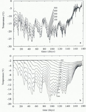
Fig. 1. (a,b) Variation of temperature with time, measured at various depths in the Antarctic sea-ice sheet. The lowest temperatures are plotted separately. The depth of the thermistor below the surface of the ice is indicated in mm by the annotations on curves, which are 100 mm apart.
(10 October). (Day 1 is 12 June 1996.) Both rising and falling temperatures are present, and the thermal conductivity may be determined directly by using the heat conduction equation
where k is the thermal conductivity of the sea ice, U is the total specific internal energy, pi is the sea-ice density (here taken to be 910 kgm−3) and T is the temperature at depth z and time t. The internal energy is given by integrating the effective heat capacity C (Sehwerdtfeger, 1963; Ono, 1966; Yen, 1981), to give
where U is in J g−1 is the average salinity of the sea ice in parts per thousand (‰), and ![]() is temperature in °C. This expression allows for the effect of latent heat as brine pockets change volume to mainta in thermodynamic equilibrium between temperature and brine concentration.
is temperature in °C. This expression allows for the effect of latent heat as brine pockets change volume to mainta in thermodynamic equilibrium between temperature and brine concentration.
Salinity measurements have been made from ice cores taken from the area studied, at the time of the experiment and at various times over the past 10 years in the McMurdo Sound area. Average salinities fall in the range 5-6‰ (except in the top 200 mm of ice), so a value of 5.5‰ was used to convert from temperature to internal energy in the following. The fitted unbiased value of thermal conductivity increased, by amounts varying from 2% near the top of the ice to 9% near the bottom of the ice, when a salinity of 6.5‰ was used as a check on sensitivity.
The non-linearity in C leads to a strong temperature de-pendence in the thermal diffusivity k/piC, and prevents use of the more usual Fourier transform method for finding k. It also prevents the substitution ![]() since this requires C to be independent of T. The emphasis is shifted then, from finding the diffusivity to finding the thermal conductivity.
since this requires C to be independent of T. The emphasis is shifted then, from finding the diffusivity to finding the thermal conductivity.
Analysis of Data
Equation (1) is fitted to the data by using finite-difference approximations to the derivatives. Central differences were used to calculate ![]() i.e.
i.e. ![]() , where Ui
is the i th value of U for a particular thermistor. The second spatial derivative
, where Ui
is the i th value of U for a particular thermistor. The second spatial derivative ![]() is approximated by
is approximated by ![]() , where Tj
is the value of T for thermistor j at a particular time. The time difference Af used is 1 hour, and the spatial difference Δz is the thermistor spacing 100 mm. The resulting numerical estimates of
, where Tj
is the value of T for thermistor j at a particular time. The time difference Af used is 1 hour, and the spatial difference Δz is the thermistor spacing 100 mm. The resulting numerical estimates of ![]() and
and ![]() are fitted with a least-squares straight line, the slope of which is k/pi
when
are fitted with a least-squares straight line, the slope of which is k/pi
when ![]() is treated as the independent variable.
is treated as the independent variable.
Values after day 110 are not used, as they are affected by solar heating. Temperatures above -5°C are not used, as models of thermal conductivity suggest that it varies rapidly with temperature in this range. Over 24 000 points remain available for filling.
In the usual simple least-squares method, the independent (x) variable is error-free. Measurement errors in x bias the fitted slope downwards (Reference FullerFuller, 1987) by a factor which is the fractional relative measurement error in X. We estimate that this factor is the same for both variables ![]() and
and ![]() , varying from about 10% near the top of the ice to 20% near the bottom. We thus fit two least-squares slopes, one with
, varying from about 10% near the top of the ice to 20% near the bottom. We thus fit two least-squares slopes, one with ![]() as the x variable and the other with
as the x variable and the other with ![]() as the x variable; the geometric mean of the two values of A; obtained is an unbiased estimate of the value of k. The uncertainty in this value of A; is estimated to be about 3%. The main source of this uncertainty is the uncertainty in estimating the measurement errors (that is, in estimating the bias); the least-squares fitting procedure gives 95% confidence limits on the fitted (biased) k values that are several orders of magnitude lower than 3%.
as the x variable; the geometric mean of the two values of A; obtained is an unbiased estimate of the value of k. The uncertainty in this value of A; is estimated to be about 3%. The main source of this uncertainty is the uncertainty in estimating the measurement errors (that is, in estimating the bias); the least-squares fitting procedure gives 95% confidence limits on the fitted (biased) k values that are several orders of magnitude lower than 3%.
Fig. 2.
A plot of ![]() (Wkg−1) against
(Wkg−1) against ![]() (°Cm−2) for the thermistor at 700 mm depth. Least-squares jits are also shown.
(°Cm−2) for the thermistor at 700 mm depth. Least-squares jits are also shown.
A typical set of data and the two fitted least-squares straight lines are plotted in Figure 2, for the thermistor at 700 mm depth. The residuals of one of these fits are plotted against spatial temperature gradient in Figure 3. An increase in variance is apparent for higher temperature gradients. This is a feature of all thermistors, and is apparent in Figure 4, which shows R 2 values vs depth, plotted separately for data with temperature gradients above and below 15°Cm−1, as well as for data with all gradients present. R 2 is the index of lit (Reference Chatterjee and PriceChatterjee and Price, 1991), and R is the correlation coefficient. R2 is a measure of flow much of the variance is accounted for by the linear fit, with a value near 1 indicating that most of the variance is accounted for and that the data are very linear in nature. Lower R2 values are consistently seen for the higher temperature gradients, indicating higher variance in these data.
Fig. 3. Residuals (data minus fit) of the lower fitted line in Figure 2, vs temperature gradient.
Figure 5 shows the geometric mean (unbiased) values of k obtained for each thermistor, plotted against depth. Circled values have R2 < 0.5, and are less reliable. Included for comparison are values for pure ice from Yen (1981), with an indication of the spread of values obtained experimentally. Temperatures for the pure ice values were obtained by averaging the temperature for each thermistor. Also shown are the fitted unbiased k values obtained when the salinity is taken to be 6.5‰. The R2 values for these fits are shown in Figure 4, and show increasing variance as depth increases, due largely to the overall linear temperature gradients established in the ice, giving smaller temperature changes near the bottom of the ice, and hence a smaller signal-to-noise ratio.
Fig. 4. The index offit vs depth. The line labelled “all” is for fits using all temperature gradients; the lines labelled “high” and “low” are for fits using temperature gradients above and below 15Cm−1, respectively.
Fig. 5. Unbiased values of thermal conductivity vs depth. Circled values have an index of fit below 0.5, and are unreliable. Results using a salinity of 5.5‰ and 6.5‰ are shown separately. The range of values from Yen (1981) for pure ice is also indicated.
The low value for k found at 200 m might be due to the higher salinities typically found at this depth.
Table 1 gives fitted values of k and R2
for each thermistor, as plotted in figures 4 and 5. Values obtained for k are generally in or below the ranges reported for pure ice, consistent with the model predictions of Sehwerdtfeger (1963). However, there is a trend towards increased values to k at greater depths (i.e. higher temperatures), the reverse of the trend for pure ice. The increased variance seen when dT/dz >15 Cm−1 suggests fitting k values separately for ![]() and
and ![]() . The results are plotted in Figure 6, and reveal no significant change in k with temperature gradient. Circled values have R2
< 0.5, and should not be given much weight.
. The results are plotted in Figure 6, and reveal no significant change in k with temperature gradient. Circled values have R2
< 0.5, and should not be given much weight.
Table 1. Unbiased (geometric mean) values of thermal con-ductivity k and index of fit R2 vs depth. Included for comparison are values for pure ice from Yen (1981)
The above results suggest that some mechanism other than conduction is contributing to heat flow through sea ice, and giving non-linear heat flow effects. These become apparent at higher temperatures (when brine volumes are larger) and at higher temperature gradients (when convec-tive effects might be larger). We suggest that the migration of brine in sea ice is a likely candidate.
The work of Lytle and Acklcy (1996) also considers the convective contributions to heat flow through sea ice. They found that brine convection occurs at very small temperature gradients, apparently in contradiction to the present work. However, their study was conducted on second-year ice, and convection through interconnected brine channels occurs even at very small temperature gradients when sea ice is warmed to near -1.8°C. Our study is on first-year ice, which does not have the initial matrix of last year's ice riddled with many brine channels found in Lytle and Aekley'S study. They also had a slush layer over the, ice, due to surface flooding of the ice and snowpack, and convection was between this slush layer and the underlying ocean.
Fig. 6. Unbiased values of thermal conductivity vs depth, plotted separately for temperature gradients above and below 15°Cm−1. Circled values have R2 < 0.5 and should be discounted. Pure ice values centre on the solid line shown.
Brine Migration and Heat Flow
Brine is known to migrate in sea ice, influenced by gravity, by internal pressure changes and by temperature gradient (Reference Kingery, Goodnow and KingeryKingery and Goodnow, 1963; Reference Hoekstra, Osterkamp and WeeksHoekstra and others, 1965; Reference JonesJones, 1973). Brine pockets move slowly towards higher temperatures, and brine moves downwards. Both directions are the same for most of our data.
Brine movement, excluding brine expulsion by pressure changes and stress cracking, is associated with latent heat of freezing and melting effects, as ice remains where brine once was. The contribution to heat flux of pockets of brine moving with velocity W is ![]() , where v
b is the volume fraction of sea ice occupied by brine, and p and L are the density and latent heat, respectively, of pure water. Pure water values are used because most of the salts remain in the brine as it migrates.
, where v
b is the volume fraction of sea ice occupied by brine, and p and L are the density and latent heat, respectively, of pure water. Pure water values are used because most of the salts remain in the brine as it migrates.
Then the heat equation is modified to
In the following, we consider what movement of brine is needed to contribute significantly to heat flow, say by the amount 2 wm −2 when ![]() = 20°Cm −1 This is 5% of the 40 wm −2 conducted by ice with a thermal conductivity of 2Wm−2 °C−1 at this temperature gradient. Using p = 1000 kg m−3, L = 350 kJ kg−1, and v
b = 0-027 corresponding to T = -10°C gives
= 20°Cm −1 This is 5% of the 40 wm −2 conducted by ice with a thermal conductivity of 2Wm−2 °C−1 at this temperature gradient. Using p = 1000 kg m−3, L = 350 kJ kg−1, and v
b = 0-027 corresponding to T = -10°C gives
so that the peak velocity of brine pockets (when tempera-lure gradients are high) would need to be aboul 2x10 −7 ms−1 to contribute this heat flow. This velocity is reasonable in its implications for desalination of sea ice. It corresponds to a peak salt flux of 6 X 10 −7 kg m−2s−1, comparable to the gravity drainage salt fluxes observed by Kingery and Goodnow (1963). So total salt balance arguments are consistent with the idea that brine movement may contribute significantly to heat flux. What is less clear is the exact nature of the mechanism responsible for the brine movement. Possible mechanisms are explored in the following subsections.
Diffusion-Driven Migration
Kingery and Goodnow (1963) distinguish between gravity drainage of salt, brine expulsion by pressure build-up, and the movement of brine pockets towards higher temperatures. A temperature gradient in the ice requires a concentration gradient in the brine pocket, and any process thai disturbs this thermodynamic equilibrium leads to freezing at the colder end of a pocket and melting at the warmer end, so that the brine migrates towards higher temperatures. Two possible processes redistributing salt concentrations in the brine are molecular diffusion and buoyancy-driven convection. The experimental evidence to dale points to molecular diffusion driving brine pocket migration (Hoekstra and others, 1965; Reference Seidensticker, Hoekstra, Osterkamp and WeeksSeidensticker, 1966). The velocities associated with this are too small to produce significant heat flows.
Hoekstra and others (1965) measured brine pocket velocities in the laboratory, finding them to scale linearly with temperature gradient, with values of about 5 μ h −1 at a temperature gradient of 20°Cm−1, two orders of magnitude loo small to produce significant heat fluxes. Larger (isolated) brine pockets, which might be subject to convective internal flow and higher migration velocities, were observed to break down into smaller poekels in their experiments.
Also, brine pocket velocities were observed to be practically independent of whether the temperature gradient was imposed in the same direction as gravity or in the opposite direction. The work of Seidensticker (1966) shows that molecular diffusion of sail, together with a careful treatment of thermal conductivity, accounts nicely for the brine pocket velocities obtained in these experiments.
Brine Convection
The laboratory experiments on brine pocket migration were on a scale that is about one-tenth that of our in-situ experiment. This small scale might remove some of the larger brine features, and not allow the feeding of brine pockets into brine channels that is observed in sea ice (Reference Niedrauer and MartinNiedrauer and Martin, 1979; Reference Weeks, Ackley and UnterstcinerWeeks and Ackley, 1986). Gravity drainage of brine is associated with brine tubes or slots, open at the bottom to seawater (Reference Lake and LewisLake and Lewis, 1970; Weeks and Ackley, 1986). Observations of fluid and salt fluxes in brine channels (Niedrauer and Martin, 1979) in sea ice suggest that the flow rates and frequency of occurrence of these channels are high enough to produce significant heat and salt fluxes. Our data show evidence of the transient effects of brine tubes on temperatures. Figure 7 is a closer view of temperatures from five adjacent thermistors near the bottom of the ice, showing evidence of a brine tube that extends about 300 mm into the ice from the sea, lowering and raising temperatures locally.
Cox and Weeks (1981) parameterise gravity drainage from sea ice based on temperature gradients. However, in their model, gravity drainage stops when the brine volumes fall below 50‰, which corresponds to temperatures below -5°C. Our data analysis excludes temperatures above —5°C, so that gravity drainage would not be significant according to I heir model. Brine expulsion remains as a likely mechanism; however, we do observe evidence of nearby brine lubes at temperatures below -5°C, as noted above.
Fig. 7. Detail of the temperature data from depths 800-1200 m near day 44, showing evidence of a nearby convecting brine tube. Annotation.S indicate depth in mm at which the temperature is taken.
Here we consider conversion in brine tubes, closed at both ends. For a vertical cylinder of fluid heated from below, the Rayleigh number is (Nicdraucr and Martin, 1979)
where ![]() is brine density, D is the molecular diffusivity of salt,
is brine density, D is the molecular diffusivity of salt, ![]() is the dynamic viscosity of the brine, g is the gravitational acceleration and r is the radius of the cylinder. The critical value of Ra for the onset of convection is 68. If Ra is below this value, there is no convection, and diffusion of salt is the dominant mechanism. Above this value, convection begins, driven by the buoyancy differences generated by the salinity gradient. We calculate that for the properties of brine at —10°C and a temperature gradient of 10°C m−1, the critical Rayleigh number is exceeded when the diameter of the brine tube is > 1 mm. This is larger than most brine pockets.
is the dynamic viscosity of the brine, g is the gravitational acceleration and r is the radius of the cylinder. The critical value of Ra for the onset of convection is 68. If Ra is below this value, there is no convection, and diffusion of salt is the dominant mechanism. Above this value, convection begins, driven by the buoyancy differences generated by the salinity gradient. We calculate that for the properties of brine at —10°C and a temperature gradient of 10°C m−1, the critical Rayleigh number is exceeded when the diameter of the brine tube is > 1 mm. This is larger than most brine pockets.
Many brine tubes are tilted at an angle to the vertical (Niedrauer and Martin, 1979), which alters their convective behaviour. Criminalc and Lelong (1984) performed a stability analysis of tilted brine drainage channels, and found two optimum angles of the channel for convection or overturn driven by brine density gradients, one being vertical, the other being at about 45°. This suggests that there is a natural preference for either vertical or 45° tubes, since at these angles the instability driving convection is strongest. All of the above analyses predict no convection in the brine tubes at small temperature gradients.
However, Reference Woods and LinzWoods and Linz (1992) showed that a slot or fracture that is inclined at some angle to the vertical, containing fluid of different thermal conductivity to the surrounding rock, will conveel at any Rayleigh number, even if the thermal gradient in the rock is stabilizing, due to tilted isotherms. They find an exact solution, which becomes singular as a critical Rayleigh number is approached. Vertical temperature gradients impose brine density gradients in brine tubes, a case covered in the work of Woods and Linz. However, their analysis (and that of Reference Criminale and LelongCriminale and Lelong, 1984) does not include the important effect of the phase change at the tube face, or allow for (or predict) the movement of the tube through the ice. Nevertheless, the mechanism driving the instability, that of tilted isotherms and isopycnals due to the different thermal conductivities of the brine and the ice, is present in sea ice, and we expect qualitatively similar results. That is, there would be no critical Rayleigh number for the onset of convection in tilted brine tubes, and convection would be observed at all gradients and in any tube no matter flow narrow.
Conclusions
Detailed temperature measurements in growing Antarctic sea ice allow the thermal conductivity to be fitted directly at a variety of temperatures, depths and gradients.
Some evidence has been presented for non-linear thermal effects in sea ice, raising the question of the importance of brine movement for heat transport. More analysis of the temperature data is planned.
Local salinity and ice-density changes with depth are unknown, and do have a significant effect on fitted thermal conductivity. Future experiments would benefit from such information, although since these properties change with time, and involve destructive methods, it is difficult to measure them in conjunction with temperature measurements.
The work of Woods and Linz (1992) raises interesting questions about whether there is a critical Rayleigh number for the onset of convection in tilted brine tubes. It is planned to extend their model to the case of brine tubes in sea ice, and to undertake a numerical and asymptotic analysis of this model.


