


Introduction
HIV/AIDS has brought tremendous challenges to global public health and life quality of humankind worldwide [Reference Xing1]. In China, a total of 769 175 patients living with HIV/AIDS were reported as of January 2018, of which 445 716 cases survived with HIV infection, 323 459 cases were AIDS patients and there were 241 519 deaths [Reference China2]. As an HIV-hit region, Guangxi Zhuang Autonomous Region, a province in southwestern China, has seen an increasing HIV incidence in recent years, and it has become a major public health problem in Guangxi [Reference Zhang3, Reference Willis4]. Therefore, corresponding intervention strategies as well as methods against local HIV/AIDS epidemics need urgently to be explored and developed. As the World Health Organization (WHO) has advocated, effective disease surveillance is dependent on effective disease control [5]. Disease surveillance can provide a decision-making basis for disease prevention and control, and can also evaluate the feasibility and effectiveness of prevention and control interventions. Nevertheless, disease surveillance data have a weakness, namely hysteresis, which means that disease surveillance reflects just the current status but has little capacity to forecast future epidemics [Reference Lyu6]. However, the government needs an accurate prediction in HIV incidence to formulate targeted interventions. Therefore, establishing high-precision prediction models is important for the monitoring and control of local HIV epidemics.
Disease forecasting plays an important role in disease prevention. Many mathematical models including linear regression, generalised linear regression, non-linear regression, decision trees, neural networks, etc. [Reference Xu7–Reference Zeng9], have been developed to predict the incidence of infectious diseases. The autoregressive integrated moving average (ARIMA) model is a classical model based on linear theory. The ARIMA model was first proposed by Box and Jenkins in the early 1970s, to predict future tendency using the past and present data of time series [Reference Box and Jenkins10]. ARIMA transforms the non-stationary time series into a stationary time series, and then establishes a regression model with the lag value of dependent variable, the present value and lag values of the random error [Reference Zheng11, Reference Zeng12]. However, the ARIMA model mainly captures a linear relationship, which may produce a large deviation for non-linear or unstable information. The generalised regression neural network (GRNN) model, which has a strong non-linear mapping ability and learning speed, has been widely used in disease prediction, modelling and estimating [Reference Wu13, Reference Kim14]. The effect of prediction is excellent when the data series is small and unstable. Furthermore, exponential smoothing (ES), a widespread method, is also a general model for analysing time series such as production forecasts and short-to-medium-term economic development trends [Reference Guan15].
In recent years, the rapid development of deep learning methods has provided an alternative approach for disease prediction [Reference Lore16]. The long short-term memory (LSTM) model, proposed first by Sepp Hochreiter and Jurgen Schmidhuber in 1997, is a neural network based on new deep learning of a recurrent neural network (RNN) [Reference Hochreiter and Schmidhuber17]. Using multi-layer and complex neural networks close to the real values, a backward propagation algorithm is used to continually shrink the fitting error [Reference Chen18]. The complex mathematical modelling and solving processes can be skipped by a cyclic neural network model based on LSTM, which is an extension of an RNN and suitable to solve the problem of correlation in time series. The LSTM includes three types of gates: the forget gate, the input gate and the output gate. These gates can be opened or closed to judge whether the result reaches the threshold and thus is to be included in the current calculation of this layer. Because of the gates, the useful data in the time series are kept, and the useless data discarded, so that the interference of useless data can be avoided and the model is more accurate in processing time series. Also, the LSTM model has been widely used in many fields, such as image recognition, speech recognition, etc. [Reference Donahue19, Reference Vinyals20]. Nevertheless, so far LSTM has rarely been used in forecasting infectious diseases, especially HIV infection. In this study, we used LSTM, ARIMA, GRNN and ES models to estimate HIV incidence in Guangxi, China, and to explore which model is the best and most precise for local HIV incidence prediction.
Methods
Ethical approval
The data came from a public-access secondary database. Formal ethical approval was not required for this study.
Data source
Data of HIV incidence in Guangxi from January 2005 to December 2016 were obtained from the public-access database of the Chinese Center for Disease Control and Prevention (CDC, http://www.phsciencedata.cn). All HIV cases of Guangxi were confirmed by clinical and laboratory tests, which were reported to the Chinese CDC within 12 h of confirmation via an Internet-based national disease-reporting system.
Construction of the ARIMA model
The ARIMA model is the most classical and commonly used model in non-stationary time-series analysis. We explored the optimal parameter values for the model using Eview 8.0 software. Construction of the ARIMA model is based on the formula as follows [Reference Zheng11]: Φ(B)(1 − B)dXτ = θ(B)ετ
In this formula, Xt represents the non-stationary values of a sequence at timet; εt is the white noise; d means differential times; B represents the backward shift operator; and θ(B) represents the moving-average operator. The ARIMA model based on the season is described as ARIMA (p, d, q)(P, D, Q)s, where p is the number of autoregressive order; d is the degree of difference; q is the sliding average order; P is the seasonal autoregressive order number; D is the degree of seasonal difference; Q is the seasonal sliding average order; and s is the number of cycles [Reference Zheng11].
Establishing an ARIMA model consists of four steps, as follows [Reference Lin21]:
Initially, time-series data were obtained from the data system.
Second, data were drawn to observe whether the time series was stationary. With regard to non-stationary time series, the d order difference operation was first performed, which was converted into a stationary time series.
Thirdly, the autocorrelation function (ACF) analysis and the partial autocorrelation function (PACF) analyses were employed to determine the possible values of p, q, P and q. Then, the models in which the parametric tests were not statistically significant (P > 0.05) were excluded, and the residual tests showed the non-white noise sequence using the Box–Jenkins Q test.
Finally, the Akaike information criterion (AIC) and Schwarz Bayesian information criterion (SBC) were used to determine the optimal model. The model with the lowest AIC and SBC values was considered as the optimal model. If the AIC and SBC values were nearly equal, the model with the higher R 2 value was selected as the optimal one.
Construction of the LSTM model
The LSTM model is virtually a neural network based on new deep learning by the RNN [Reference Hochreiter and Schmidhuber17]. In this study, we used Anaconda based on Python 3.5 programming to develop the LSTM model. The calculation node [Reference Dvornek22] is shown in Figure 1.
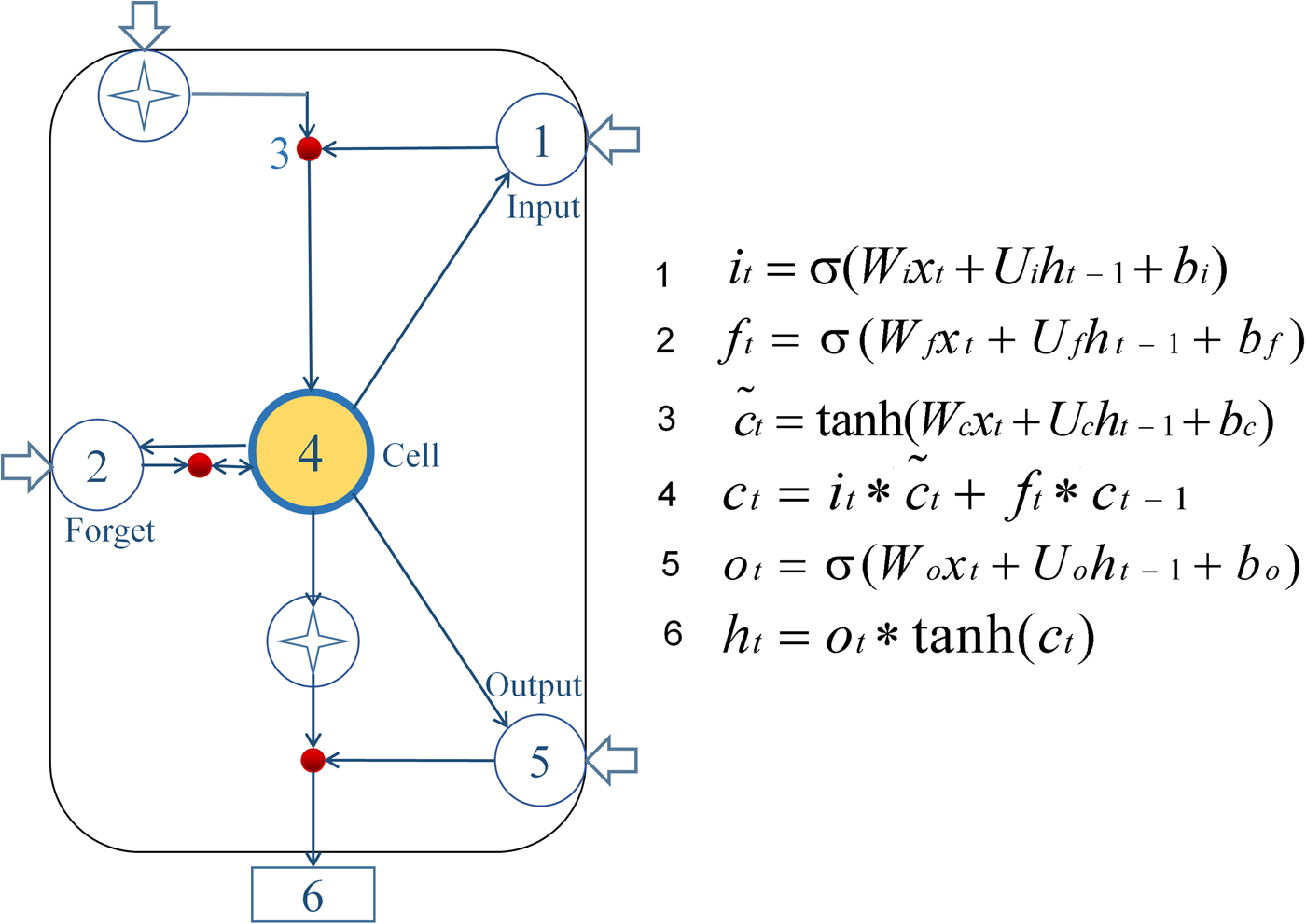
Fig. 1. Diagram of LSTM neural network pattern. Input gate (it) determines which information needs to be updated in the unit state; the forgetting gate (ft) controls information which needs to be discarded from the unit state; then input gate and a vector  $(\widetilde{c}_t)$ are created by Tanh to determine which new information is stored in the unit state to update the old unit state, and turn into the new unit state (ct). Finally, cell state information is filtered with the output gate (ot) to update the hidden state (ht), which is the output of the LSTM cell.
In the formulas, the input gate (i t) determines which information needs to be updated in the unit state; and the forget gate (ft) controls information which needs to be discarded from the unit state. Next, the input gate and a vector  $(\widetilde{c}_t)$ are created by Tanh to determine which new information is stored in the unit state to update the old unit state, and turn it into the new unit state (ct). Finally, cell state information is filtered with the output gate (ot) to update the hidden state (ht), which is the output of the LSTM cell [Reference Greff23, Reference Gers24]. Briefly, the LSTM designed a structure to remove or add elements to the cell state called gates. The information was selected by these gates, which are composed of a sigmoid neural network layer and a scalar multiplication operation. The sigmoid layer outputs a value between 0 and 1, indicating how many components could pass, 0 means ‘no information can pass’, while 1 means ‘all information can pass’. Each gate is responsible for different tasks, and the forget gate is responsible for deciding how many cell states are reserved from the previous moment to the current moment. The input gate is responsible for deciding how many cell states are reserved from the current moment to the current moment; and the output gate is responsible for determining how much output the cell state has at the current time. In these formulas, the W matrices show the weight applied to the current input, the U matrices represent the weight applied to the previous hidden state, the b vectors are biases for each layer and σ is the sigmoid function. Establishing the LSTM model consisted of three steps:
Initially, the raw data were divided into two parts: data of the last 2 years were considered as the test set, and the rest data were used as a training set. The training samples were used to build the model and to discover potential relationships in the data, and the test samples were used to evaluate the predictive power of the model constructed by the training set.
Subsequently, a series of LSTM models were constructed using N values which were the time steps. For example, if the time step was 20, the value of the 21st data was predicted with the last 20 data as input. The model with the lowest mean square error (MSE) was considered the optimal model.
Finally, the incidence was predicted by the optimal model for the assignment of the lowest MSE.
Construction of the GRNN model
The GRNN model, first proposed and developed by Specht [Reference Specht25], has a strong non-linear mapping ability and learning speed. The predictive effect is excellent when the data series is small and unstable data are also solved. The GRNN consists of four layers: an input layer, a pattern layer, a summation layer and an output layer [Reference Ghritlahre and Prasad26, Reference Wang27]. The input layer inputs sample data and the pattern layer calculates the Gauss value for each of the test and training samples. The summation layer consists of two nodes, the first is the output sum of each hidden layer node, and the second is the weighted sum of proleptic results and each hidden layer node. The output layer outputs the result of dividing two nodes from the third layer [Reference Singh28]. The method and steps have been previously described in detail [Reference Wei29].
Construction of the ES model
The ES model is also a general method for analysing time series [Reference Guan15, Reference Ke30]. It has a widespread use in the production of forecasting and also used for short-to-medium-term economic development trends. As a special form of the weighted average method, the ES method does not need to conduct a quantitative research on the internal factors and relations of systems, but to observe valuable information from the data itself. Establishing an ES model consists of three steps as follows [Reference Pereira31]:
Initially, determining the initial values. If the time series had more original data, the original data were used to replace the initial value of the ES method; if the time series had fewer data, the average value of the original data was taken as the initial value.
Subsequently, selecting the smoothing factor α and calculating the ES values. The value of α determines the smoothing level and response speed to the difference between the predicted and actual values. When the time series was relatively stable, a smaller smoothing factor was obtained; otherwise, a larger smoothing factor was adopted.
Finally, the smoothing factor, which a minimised MSE, was determined and the predicted values were obtained.
Patient and public involvement
Neither was involved.
Results
Construction of ARIMA models
For ARIMA model construction, monthly HIV incidence from January 2005 to December 2014 was used; for testing the predictive ability of these models, HIV incidence in 2015 or 2016 was used. Figure 2 shows the monthly HIV incidence from January 2005 to December 2015 in Guangxi, China. Overall, the HIV incidence exhibited a seasonal tendency (s = 12) (Fig. 2). From 2005 to 2011, the HIV incidence in Guangxi increased slowly, but the epidemic situation from 2011 to 2015 showed a slow and seasonal decline, which meant that the time series was not stationary. Thus, the data were processed by a log transformation with non-seasonal (d = 1) and seasonal difference (D = 1), to remove numerical instabilities. After data processing, the ADF test showed a statistically significant result (P < 0.0001), indicating that the time sequence was stationary (Supplementary Table S1).

Fig. 2. Monthly incidence of HIV in Guangxi, China (from January 2005 to December 2015). According to the trend section, it can be found that the incidence of HIV shows seasonal tendency (s = 12). From 2005 to 2011, the HIV incidence in Guangxi was increasing slowly, and the epidemic situation in 2011–2016 showed a seasonal slow decline.
The ACF and PACF analyses were then used to determine the parameters of the ARIMA models (Supplementary Fig. S1). According to the results of the ACF and PACF analyses (however, some models were not tested by parameters or residuals), three appropriate models, namely, ARIMA (2, 1, 0) (1, 1, 2)12, ARIMA (2, 0, 1) (0, 1, 2)12 and ARIMA (0, 1, 0) (2, 1, 2)12, were identified to predict the HIV incidence in 2016. These three models had approximate AIC and SBC values (Supplementary Table S2). However, the model ARIMA (2, 1, 0) (1, 1, 2)12 had a higher R 2 than the other two, and it was selected as the optimal model. Supplementary Tables S3 and S4 list the parameter test results of the best prediction model, which showed the white noise sequence in 2015 and 2016, respectively. The forecasting curve of the optimal ARIMA model and the actual HIV incidence curve are shown in Figure 4.
Construction of LSTM models
A multiple neural network architecture which relied on the LSTM layer was used to predict the HIV incidence in 2015 and 2016 using Python programming. HIV incidence data from 2005 to 2014 were used as the training set to construct the LSTM models, and the 2015 data were applied as test sets to evaluate the fitting capacity of the LSTM models. In the same way, the incidence in 2016 was predicted by the data from 2005 to 2015. Before setting up the LSTM forecasting system, the parameters (N) were set as shown in Figure 3. The MSE in different N values were then determined using HIV incidence in 2015 and 2016, respectively (Fig. 3). The LSTM model when the value of N was 12 had the lowest MSE value, and it was selected as the optimal model (Fig. 3). The forecasting curve of the optimal LSTM model and the actual HIV incidence curve are shown in Figure 4.
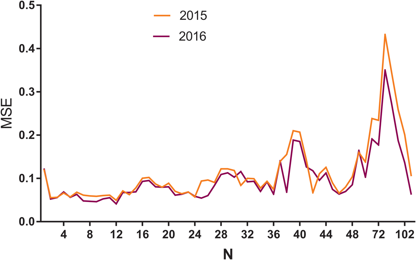
Fig. 3. The MSE of LSTM models with different N values using HIV incidence in 2015 and 2016. MSE, mean square error; N: the number of input to the LSTM model. The yellow line means N value and corresponding MSE in 2015, while the purple line means N and MSE in 2016. As can be seen from the figure, when the N was 12, the model had the minimum MSE in 2015 and 2016.
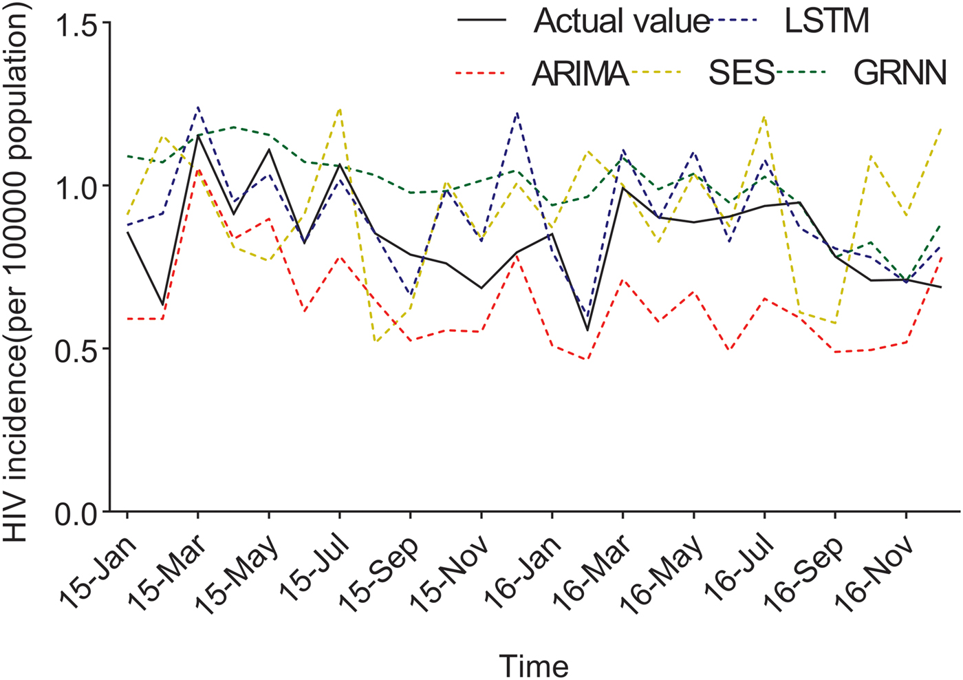
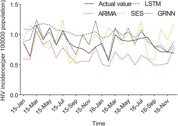
Fig. 4. The forecasting curves of the optimal LSTM and other models as well as the actual HIV incidence series. Comparison of LSTM model and other models. LSTM, the long short-term memory neural network model; ARIMA, the autoregressive integrated moving average model. The black line means the actual data, the blue dashed line means the predictive data via the LSTM model, the red dashed line means the predictive value via the ARIMA model, the yellow dashed line means the predictive value via the SES model, while the green dashed line means the predictive value via the GRNN model. Compared with ARIMA, SES and GRNN, the predicted value of LSTM was closer to the actual value.
The predicted values of the optimal LSTM and ARIMA models were compared with the actual HIV incidence in Guangxi in 2015 and 2016, respectively. As shown in Figure 4, forecasting results by the LSTM model were closer to the actual values than those of ARIMA, GRNN and ES models. Furthermore, four performance metrics (MSE, root mean square error (RMSE), mean absolute error (MAE) and mean absolute percentage error (MAPE)) of the LSTM model were all lower than those of the other models (Table 1). Therefore, the LSTM neural network model was superior in predicting the incidence of HIV in Guangxi.
Table 1. Performance of LSTM and the other models in 2015 and 2016

MSE, mean square error; RMSE, root mean square error; MAE, mean absolute error; MAPE, mean absolute percentage error.
Construction of GRNN models
The time series from January 2005 to December 2015 was selected to develop the network. Incidences of November 2016 and December 2016 were selected as the testing samples and the rest were used to train the network. The optimal N value of GRNN was 18; namely, a basic model with 18-dimensional input and one-dimensional output showed the minimum RMSE. The forecasting curve of the optimal GRNN model and the actual HIV incidence curve are shown in Figure 4 and the four performance metrics (MSE, RMSE, MAE and MAPE) are shown in Table 1.
Construction of ES models
ES and seasonal ES methods were developed by JMP 13. As shown in Supplementary Table S2, the R 2 of the seasonal ES model was higher, and the AIC and SBC were lower. The estimation of the parameters of these methods is shown in Supplementary Table S5. MSE, RMSE, MAE and MAPE of the seasonal ES model were all higher than other models.
Discussion
The HIV epidemic is still severe in Guangxi, and it is necessary to establish an effective monitoring network for the prevention and control of HIV. In the present study, various models for analysing the time series: LSTM, ARIMA and ES were established using the 10-year historical HIV incidence data, and their predictive abilities were compared. We found that the LSTM model had better predictive ability than did ARIMA and other models, which is largely consistent with the results reported by others in predicting the influenza outbreaks [Reference Zhang and Nawata32].
Different models have their own merits and faults. The ARIMA model includes a moving average process, an autoregressive moving average process, an autoregressive moving average process and an ARIMA process according to the different parts of the regression and whether the original data are stable. The model is very simple and requires only endogenous, rather than exogenous, variables. But the limitations of ARIMA model were shown to be as follows: (1) the time series must be stationary or stable after difference; and (2) only linear relationships could be captured [Reference Zheng11, Reference Wei29]. In our study, the ARIMA model showed a large difference in predicting HIV incidences in 2015 and 2016 (Fig. 4). Although ARIMA is a classic model that is widely used to predict the initiation and epidemic progression of infectious diseases, the reason might be that the HIV incidence in Guangxi exhibits a seasonal tendency. Besides, the incidence increased slowly from 2005 to 2011, and the epidemic situation from 2011 to 2015 showed a slow and seasonal decline. However, the LSTM model can model the data of a time series, particularly the long-term data, and automatically determine the optimal time lag [Reference Ordonez and Roggen33]. Like most RNNs, the LSTM network is universal, because if enough network units are provided, it can compute anything that the conventional computer can, as long as the proper weight matrix is provided. An LSTM network is well-suited to process and predict the time series when there are very long time lags of unknown size. Thus, LSTM is a more effective and extensible learning model for continuous data than is ARIMA. The GRNN model was developed as a new potential tool for infectious disease incidence prediction. It is characterised by a fast convergence and good non-linear approximation performance based on a radial basis network. However, because each test sample needs to be calculated, the GRNN model has to store all the training samples, which increases the spatial complexity [Reference Ghritlahre and Prasad26]. In our study, the GRNN model had lower performance metrics than the other models, which means it is not an outstanding model to predict the incidence of HIV in Guangxi. ES is also a widely used method for analysing the time series. It does not discard the data in the past, and only gradually decreases the degree of influence [Reference Ke30]. Briefly, the weight gradually converges to zero. Nevertheless, ES lacks the ability to identify the transition of data, and the long-term prediction is poor. In this study, the seasonal ES method showed a large difference in predicting the incidence because the tendency of the original data was intricate.
The characteristics of the HIV/AIDS epidemic in Guangxi are shown to be as follows: (1) the number of cases, diseases and the ratio of late detection were overall high; (2) the proportion of farmers and student cases was increasing year by year, the proportion of individuals over 50 years of age was obviously rising, and the proportion of heterosexual transmission was over 92% in the last 4 years; and (3) a large number of local cases, and new findings and reports indicated that the morbidity had already shifted from high-risk groups to the general population [Reference Ge34]. From 2006 to 2010, the HIV/AIDS entered the stage of the widespread epidemic, in which HIV-1 transmission in Guangxi was dominated by heterosexual transmission, and the tendency from high-risk groups to the general population was obvious. Then, Guangxi accessed the implementation stage of the HIV-1 prevention project from 2011 to 2016, and the fluctuation of HIV incidence declined slowly. This is consistent with the trend in China.
Although the effectiveness of the LSTM model in this study is sufficient and the model is feasible, there are still small deviations between the predicted results and the actual values. The source of these differences might come from a number of influencing factors, including the environmental and behavioural factors, and the intensity of intervention in different areas, etc. [Reference Harrison35, Reference Alvarez-Uria36]. After all, for the LSTM model, time series is the only variable, and other influencing factors could not be included in the model. In addition to the influencing factors mentioned above, there is also a special factor for the HIV/AIDS epidemic in Guangxi, the foreign immigrants and tourists. Guangxi is a border province in China, and is geographically close to the Association of Southeast Asian Nations (ASEAN) countries. The number of immigrants and tourists has increased greatly in recent years, especially those from neighbouring Vietnam [Reference Bo and Yufang37, Reference Huo38]. Some studies have shown that female sex workers from Vietnam have spread Vietnam's endemic HIV-1 strains to Guangxi and contributed to the local epidemic [Reference Zhu39, Reference Wang40]. However, this contribution is actually in a node and could not be reflected in the LSTM model. Overall, although the LSTM model in this study has a relatively good effect and predictive ability, more advanced disease forecast models that can include multiple factors need further development in the near future, to make the forecasting more precise and closer to the truth.
Conclusions
In this study, four types of models, LSTM, ARIMA, GRNN and ES, were established and their predictive abilities compared. The LSTM model was a better predictive model than the others in forecasting the HIV incidence. Establishing an LSTM model is important for the monitoring and control of the local HIV epidemic in Guangxi, China.
Supplementary material
The supplementary material for this article can be found at https://doi.org/10.1017/S095026881900075X
Author ORCIDs
Li Ye, 0000-0001-7688-4867.
Acknowledgements
This study was partially supported by the National Key Science and Technology Project of China (grant no. 2018ZX10101002-001-006). Moreover, the authors would like to express their gratitude to all those who have dedicated to the surveillance, laboratory testing for notifiable infectious diseases in Guangxi and China.
Author contributions
Conceived and designed the study: G. Wang, W. Wei, H. Liang and L. Ye; performed the data collection: G. Wang and W. Wei; data analysis and building analysis tools: G. Wang and W. Wei; writing and revising the manuscript: G. Wang, W. Wei, H. Liang, L. Ye, J. Jiang, C. Ning, H. Chen, J. Huang, B. Liang, N. Zang, Y. Liao, R. Chen, J. Lai and O. Zhou.
Financial support
This study was supported by the Guangxi University ‘100-Talent’ Program & Guangxi university innovation team and outstanding scholars programme (Gui Jiao Ren 2014 [Reference Xu7]), the Guangxi Scientific and Technological Development Project (Gui Ke Gong 14124003-1), the Basic Ability Improvement Program for Young and Middle-aged Teachers of Guangxi Universities (No: 2017KY0105) and the National Natural Science Foundation of China (8180121000, 81760602).
Conflict of interest
None.


 Open access