


1. Introduction
Streaks of small particles are formed when suspended particles interact with a turbulent boundary layer. This phenomenon can be observed in the atmospheric surface layer (ASL) where, under certain environmental conditions, dust or sand forms so-called aeolian streamers, i.e. elongated regions of visibly large concentration, with typical widths  ${\sim }20$ cm and spanwise spacing ${\sim }1$ m (Baas & Sherman Reference Baas and Sherman2005; Baas Reference Baas2008; Sherman et al. Reference Sherman, Houser, Ellis, Farrell, Li, Davidson-Arnott, Baas and Maia2013; Baas & van den Berg Reference Baas and van den Berg2018). An open question is whether such streamers are formed directly by erosion from the ground, or by confluence of particles already suspended in the flow. The leading hypothesis based on field measurements is formation by pointwise erosion (Baas & Sherman Reference Baas and Sherman2005; Baas Reference Baas2008). However, the detailed mechanisms of flow–particle interaction remain elusive, our understanding hindered by limitations in measurement techniques. Optical approaches have high resolution but typically limited field of view, while point-based sensors can cover larger areas but have insufficient spatial resolution. Moreover, to elucidate the two-phase interaction, high-resolution simultaneous measurements of both fluid and particle phase would be necessary; but these appear prohibitively difficult to perform in the outdoor field. As an alternative to field measurements, the ASL can be modelled as a high-Reynolds-number version of a canonical flat plate turbulent boundary layer (Hutchins et al. Reference Hutchins, Chauhan, Marusic, Monty and Klewicki2012), which can be studied using numerical simulations or laboratory experiments.
Numerical simulations have indicated a connection between the spatial distribution of suspended particles and coherent structures in wall-bounded flows. McLaughlin (Reference McLaughlin1989) showed that particles form streaks by aggregating in the elongated regions of relatively low fluid velocity. The latter, often called near-wall streaks or low-speed streaks, have long been recognized as signature features of wall turbulence (Kline et al. Reference Kline, Reynolds, Schraub and Runstadler1967; Robinson Reference Robinson1991). Marchioli & Soldati (Reference Marchioli and Soldati2002) found that particles statistically oversample sweeps (defined by positive streamwise velocity fluctuations and negative wall-normal velocity fluctuations) and ejections (negative streamwise fluctuations and positive wall-normal fluctuations). As sweep/ejection pairs are typically associated with hairpin vortices (Adrian, Meinhart & Tomkins Reference Adrian, Meinhart and Tomkins2000b), the formation of particle streaks appeared to be related to such coherent structures. The interaction of suspended particles with coherent structures in the flow was further evidenced by the observation that particles tend to form streaks when their Kolmogorov-scaled Stokes number is of order unity (Rouson & Eaton Reference Rouson and Eaton2001), mimicking scale-dependent interactions and clustering well-known for homogeneous turbulence (Eaton & Fessler Reference Eaton and Fessler1994; Yoshimoto & Goto Reference Yoshimoto and Goto2007). As a result of this scale dependence, Wang & Richter (Reference Wang and Richter2020) found that the response of particles to different-sized flow structures in the turbulent boundary layer depends on particle inertia. Similarly, Jie et al. (Reference Jie, Cui, Xu and Zhao2022) observed the formation of small-scale and large-scale streaks for particles with small and large response time, respectively. Motoori, Wong & Goto (Reference Motoori, Wong and Goto2022) also highlighted the interaction of inertial particles with vortices having turnover times close to their response times. The correlation of particle streaks with specific flow structures was confirmed by numerous numerical studies (e.g. Zhang & Ahmadi Reference Zhang and Ahmadi2000; Picciotto, Marchioli & Soldati Reference Picciotto, Marchioli and Soldati2005; Picano, Sardina & Casciola Reference Picano, Sardina and Casciola2009; Soldati & Marchioli Reference Soldati and Marchioli2009; Sardina et al. Reference Sardina, Picano, Schlatter, Brandt and Casciola2011, Reference Sardina, Schlatter, Brandt, Picano and Casciola2012; Nilsen, Andersson & Zhao Reference Nilsen, Andersson and Zhao2013; Richter & Sullivan Reference Richter and Sullivan2013; Bernardini Reference Bernardini2014; Wang & Richter Reference Wang and Richter2019). It was found that particle streaks are separated by  ${O}(100)$ viscous wall units (i.e. normalizing the distance by the kinematic viscosity $\nu$ and friction velocity $u_\tau$), which correspond approximately to the spanwise separation of near-wall streaks in wall-bounded flows (Robinson Reference Robinson1991). While these simulations concern fully suspended particles and thus cannot address the role of bed erosion, they indicate clearly that specific flow structures can induce the formation of particle streaks, which may explain (at least in part) the observation of aeolian streamers.
While numerical simulations have greatly deepened our understanding of particle– turbulence interactions in turbulent boundary layers, they suffer from two major limitations. First, most of the works referenced above treat particles as material points, following the framework of Maxey & Riley (Reference Maxey and Riley1983) and Gatignol (Reference Gatignol1983). This relies on restricting assumptions that limit its applicability, in particular when the particle Reynolds number is not small (Maxey Reference Maxey2017; Wang et al. Reference Wang, Fong, Coletti, Capecelatro and Richter2019; Brandt & Coletti Reference Brandt and Coletti2022). Specifically for wall-bounded flows, the high velocity gradients may result in significant lift forces (Costa, Brandt & Picano Reference Costa, Brandt and Picano2019) that are neglected in most point-particle simulations. When the particle back-reaction on the fluid is taken into account, the point-particle approach contains well-known uncertainties related to the pointwise forcing on the computational grid (Eaton Reference Eaton2009; Balachandar & Eaton Reference Balachandar and Eaton2010). While advanced strategies have been proposed to overcome these shortcomings (Capecelatro & Desjardins Reference Capecelatro and Desjardins2013; Gualtieri et al. Reference Gualtieri, Picano, Sardina and Casciola2015; Horwitz & Mani Reference Horwitz and Mani2016; Ireland & Desjardins Reference Ireland and Desjardins2017; Balachandar, Liu & Lakhote Reference Balachandar, Liu and Lakhote2019), no generally accepted method has yet emerged.
Second, numerical simulations are confined to relatively low Reynolds numbers. Most studies are limited to friction Reynolds numbers  $Re_\tau = u_\tau \delta /\nu =O(10^2)$ (where $\delta$ is the boundary layer thickness), significantly constraining the range of structures in the flow. At these regimes, the flow is dominated by near-wall streaks that follow viscous scaling. For higher Reynolds numbers (typically $Re_\tau >2000$), in addition to the near-wall streaks, elongated large-scale motions are found further away from the wall (Hutchins & Marusic Reference Hutchins and Marusic2007; Smits, McKeon & Marusic Reference Smits, McKeon and Marusic2011). Because the importance of large-scale motions and their separation from the near-wall streaks grows with Reynolds number (Smits et al. Reference Smits, McKeon and Marusic2011), the former are expected to be predominant in the ASL, where typically $Re_\tau = O(10^6)$ (Wang & Zheng Reference Wang and Zheng2016). As a result, the particle–turbulence interaction of low-Reynolds-number flows may not be representative of large-scale phenomena observed in the ASL. The few numerical investigations of particle-laden wall turbulence reaching $Re_\tau = O(10^3)$ (Sardina et al. Reference Sardina, Schlatter, Brandt, Picano and Casciola2012; Bernardini Reference Bernardini2014; Li, Luo & Fan Reference Li, Luo and Fan2017; Wang & Richter Reference Wang and Richter2020; Jie et al. Reference Jie, Cui, Xu and Zhao2022; Motoori et al. Reference Motoori, Wong and Goto2022; Gao, Samtaney & Richter Reference Gao, Samtaney and Richter2023; Motoori & Goto Reference Motoori and Goto2023) used the point-particle approach, and neglected gravity. While the latter may appear as a reasonable assumption when the particle fall speed is much smaller than the advection velocity, gravity was shown to crucially change the dynamics even for particles of small inertia. This was demonstrated for light and heavy particles in homogeneous turbulence (Ireland, Bragg & Collins Reference Ireland, Bragg and Collins2016; Mathai et al. Reference Mathai, Calzavarini, Brons, Sun and Lohse2016; Berk & Coletti Reference Berk and Coletti2021) and for heavy particles in wall-bounded turbulence (Lee & Lee Reference Lee and Lee2019; Bragg, Richter & Wang Reference Bragg, Richter and Wang2021).
More recently, interface-resolved simulations have allowed simulation of the particle–fluid interaction in wall-bounded turbulent flows without resorting to simplified models (e.g. García-Villalba, Kidanemariam & Uhlmann Reference García-Villalba, Kidanemariam and Uhlmann2012; Picano, Breugem & Brandt Reference Picano, Breugem and Brandt2015; Lin et al. Reference Lin, Shao, Yu and Wang2017; Wang, Abbas & Climent Reference Wang, Abbas and Climent2017; Costa et al. Reference Costa, Brandt and Picano2019; Scherer et al. Reference Scherer, Uhlmann, Kidanemariam and Krayer2021). This approach, however, is computationally expensive and therefore limited to relatively low Reynolds numbers and small numbers of particles. On the other hand, a growing number of studies use large eddy simulations (LES) which can reach realistic Reynolds numbers found in the ASL (Jacob & Anderson Reference Jacob and Anderson2016; Zheng, Feng & Wang Reference Zheng, Feng and Wang2021; Hu, Johnson & Meneveau Reference Hu, Johnson and Meneveau2023). However, as of yet, accepted LES models that describe the subgrid-scale particle–flow interactions are lacking (Kuerten Reference Kuerten2016; Liu & Zheng Reference Liu and Zheng2021).
Limitations in field measurements and numerical simulations highlight the importance of well-controlled laboratory experiments. Investigations on the interaction of inertial particles with wall-bounded turbulence in air were performed in channels (Fessler, Kulick & Eaton Reference Fessler, Kulick and Eaton1994; Kulick, Fessler & Eaton Reference Kulick, Fessler and Eaton1994; Kussin & Sommerfeld Reference Kussin and Sommerfeld2002; Khalitov & Longmire Reference Khalitov and Longmire2003; Benson, Tanaka & Eaton Reference Benson, Tanaka and Eaton2005; Li et al. Reference Li, Wang, Liu, Chen and Zheng2012; Fong, Amili & Coletti Reference Fong, Amili and Coletti2019) and pipes (Caraman, Borée & Simonin Reference Caraman, Borée and Simonin2003; Hadinoto et al. Reference Hadinoto, Jones, Yurteri and Curtis2005). A number of groups investigated the interaction of solid particles with wall-bounded turbulence in water (Kaftori, Hetsroni & Banerjee Reference Kaftori, Hetsroni and Banerjee1995a,Reference Kaftori, Hetsroni and Banerjeeb; Niño & Garcia Reference Niño and Garcia1996; Kiger & Pan Reference Kiger and Pan2002; Righetti & Romano Reference Righetti and Romano2004; Rabencov, Arca & van Hout Reference Rabencov, Arca and van Hout2014; Oliveira, van der Geld & Kuerten Reference Oliveira, van der Geld and Kuerten2017; Shokri et al. Reference Shokri, Ghaemi, Nobes and Sanders2017; Ebrahimian, Sanders & Ghaemi Reference Ebrahimian, Sanders and Ghaemi2019; Baker & Coletti Reference Baker and Coletti2021; Cui, Ruhman & Jacobi Reference Cui, Ruhman and Jacobi2022). In this case, unlike in aeolian transport, the particle-to-fluid density ratio is  $O(1)$ and the particles are typically larger than the viscous scales. Some basic features are observed using both working fluids, in particular the oversampling of sweep/ejection events (Kiger & Pan Reference Kiger and Pan2002; Baker & Coletti Reference Baker and Coletti2021), consistent with numerical findings. Still, the experimental observations of particle streaks have been sporadic and limited to mostly snapshot realizations (Kaftori et al. Reference Kaftori, Hetsroni and Banerjee1995a,Reference Kaftori, Hetsroni and Banerjeeb; Niño & Garcia Reference Niño and Garcia1996). Only recently, Fong et al. (Reference Fong, Amili and Coletti2019) documented quantitatively the spatial extent of particle streaks, and confirmed for them a spanwise spacing of $O(100)$ wall units.
Similar to numerical simulations, most laboratory studies in channel and pipe flows suffer from limitations in terms of Reynolds number, which typically do not warrant significant separation between near-wall and large-scale motions. Wind tunnel studies have reached higher Reynolds numbers in turbulent boundary layers. Tanière, Oesterlé & Monnier (Reference Tanière, Oesterlé and Monnier1997) considered inertial particles at  $Re_\tau = 1700$, but reported only wall-normal profiles of single-point statistics. More recent studies have used two-dimensional imaging, which can capture the spatial organization of the flow. Zhu et al. (Reference Zhu, Pan, Wang, Liang, Ji and Wang2021) identified inclined clusters of particles along streamwise/wall-normal planes at $Re_\tau =5500$. Based on their orientation and self-similar properties, they proposed a conceptual model in which these clusters are driven by wall-attached eddies. In Berk & Coletti (Reference Berk and Coletti2020), we investigated the two-phase dynamics along streamwise/wall-normal planes in a turbulent boundary layer up to $Re_\tau =19\,000$. We confirmed that inertial particles oversample ejections, and highlighted the limitations of the classic theory by Rouse (Reference Rouse1937) and Prandtl (Reference Prandtl1952) to predict the wall-normal profile of particle concentration. Elongated particle streaks are better captured by imaging wall-parallel planes. This was realized in the water tunnel measurements of Cui et al. (Reference Cui, Ruhman and Jacobi2022), who analysed the spatial distribution of particles within the logarithmic region of a turbulent boundary layer at $Re_\tau =2150$. They found elongated structures of streamwise and spanwise size consistent with the large-scale motions.
With mounting evidence that particle streaks are driven by coherent flow structures in wall-bounded turbulence, the spatial extent of particle streaks can be expected to match that of those structures. In this regard, however, field observations offer a seemingly contradictory picture. Consider the spanwise scale of the most energetic structures in the turbulent boundary layer, i.e. near-wall streaks and large-scale motions. The former (figure 1a) have approximate widths  $\lambda _z^+\sim 100$ (Kline et al. Reference Kline, Reynolds, Schraub and Runstadler1967; Smits et al. Reference Smits, McKeon and Marusic2011; Wang, Pan & Wang Reference Wang, Pan and Wang2018), where the superscript ‘ $+$’ indicates normalization in wall units, while the latter have approximate widths $\lambda _z/\delta \sim 0.5$ (Hutchins et al. Reference Hutchins, Monty, Ganapathisubramani, Ng and Marusic2011) (figure 1c). Here and in the following, $z$ indicates the spanwise direction, while $x$ and
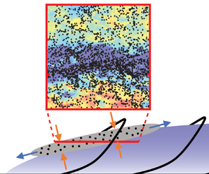
  $y$ indicate the streamwise and wall-normal directions, respectively. Under typical conditions in the ASL, these scales correspond to approximately 2 cm for the near-wall streaks, and 30 m for the large-scale motions (estimated using parameters from Klewicki et al. Reference Klewicki, Metzger, Kelner and Thurlow1995; Metzger & Klewicki Reference Metzger and Klewicki2001). In contrast, the characteristic spanwise extent of aeolian streamers is an order of magnitude larger than the former, and smaller than the latter (figure 1(b); see Baas & Sherman Reference Baas and Sherman2005; Baas Reference Baas2008; Sherman et al. Reference Sherman, Houser, Ellis, Farrell, Li, Davidson-Arnott, Baas and Maia2013; Baas & van den Berg Reference Baas and van den Berg2018).

Figure 1. Spanwise scales of (a) near-wall streaks (adapted from Kline et al. Reference Kline, Reynolds, Schraub and Runstadler1967), (b) aeolian streamers (adapted from Baas Reference Baas2008), and (c) large-scale motions (adapted from Marusic, Mathis & Hutchins Reference Marusic, Mathis and Hutchins2010a).
The above suggests that aeolian streamers in the ASL, and particle streaks in general, are driven by coherent structures spanning a range of scales. This is consistent with the framework of the attached eddy model, which describes the turbulent boundary layer as a collection of self-similar eddies (Townsend Reference Townsend1956; Perry, Henbest & Chong Reference Perry, Henbest and Chong1986; Marušić & Perry Reference Marušić and Perry1995; Marusic & Monty Reference Marusic and Monty2019). These are usually interpreted as statistical representations of hairpins and hairpin packets, or alternatively as uniform momentum zones separated by internal shear layers (Dennis & Nickels Reference Dennis and Nickels2011; Heisel et al. Reference Heisel, Dasari, Liu, Hong, Coletti and Guala2018). Due to their extremely large range of scales, atmospheric flows lend themselves especially well to being described by the attached eddy model. Indeed, recent field studies found flow structures in the ASL consistent with such a framework (Heisel et al. Reference Heisel, Dasari, Liu, Hong, Coletti and Guala2018; Hu, Yang & Zheng Reference Hu, Yang and Zheng2019; Puccioni et al. Reference Puccioni, Calaf, Pardyjak, Hoch, Morrison, Perelet and Iungo2023).
In conclusion, numerical simulations indicate that particles in wall-bounded flows form elongated streaks driven by coherent turbulent structures, with scales that depend on the particle response time. However, several shortcomings (representation of the dispersed phase, relatively low Reynolds numbers, neglect of gravity) suggest caution in extending the computational findings to large-scale/atmospheric flows. On the other hand, direct experimental evidence on particle streaks and their relation to flow structures is scarce. Remarkably, only two recent papers, Fong et al. (Reference Fong, Amili and Coletti2019) and Cui et al. (Reference Cui, Ruhman and Jacobi2022), characterized particle streaks quantitatively. However, they were not directly relevant to atmospheric flows (due to the direction of gravity and the fluid-to-solid density ratio, respectively), nor did they investigate the relation between particle streaks and the underlying turbulence. Therefore, several outstanding questions remain unanswered. What is the spatial extent of particle streaks in high-Reynolds-number flows? How does it depend on the particle inertia? What is the quantitative connection between particle streaks and the underlying coherent structures?
In the present work, we attempt to address these questions by investigating particle-laden turbulent boundary layers in a large-scale wind tunnel at  $Re_\tau = O(10^4)$. While not as high as in the ASL, the Reynolds number is sufficient to ensure significant scale separation between near-wall streaks and large-scale motions. The present study is therefore an intermediate step between the current body of lower-Reynolds-number literature and the full-scale ASL. By simultaneous two-phase imaging along wall-parallel planes, we obtain quantitative characterization of, and insight into, the interaction of the inertial particles with specific structures of the flow. The paper is organized as follows. The experimental methodology is described in § 2. In § 3.1, we identify low-speed structures in the flow and show their statistical association to high particle concentration. In § 3.2, we consider the particles’ velocities, their slip with respect to the fluid, and its relation with the particle concentration. In § 3.3, we characterize the streaks’ geometric properties. In § 3.4, we analyse the topology of the flow sampled preferentially by the particles, and deduce from it a scaling argument that agrees with the laboratory measurements and is consistent with field observations. Conclusions are drawn in § 4.
2. Experimental methods
2.1. Experimental apparatus and measurement approach
The set-up and procedures were described in Berk & Coletti (Reference Berk and Coletti2020) and are described only briefly here. Experiments are performed in the boundary layer wind tunnel at St Anthony Falls Laboratory, University of Minnesota. The cross-section is 1.7 m by 1.7 m, allowing for a thick turbulent boundary layer that grows for 16 m in approximately zero-pressure-gradient conditions. Inertial particles and flow tracers are seeded simultaneously in the flow. The tracers (1– $2\ \mathrm {\mu }$m DEHS droplets) are introduced before the contraction section of the wind tunnel using multiple Laskin nozzles. The inertial particles are size-selected glass spheres (Mo-Sci Corp., characterized in Petersen, Baker & Coletti Reference Petersen, Baker and Coletti2019), injected into the boundary layer at the spanwise centre of the wind tunnel, downstream of the boundary layer trip and 11.3 m upstream of the measurement location. In the considered regimes, the particles remain fully suspended in the flow. At the measurement location, the particle-laden flow is approximately in equilibrium, with no measurable vertical particle flux or spatial/temporal variations of the statistics.
The flow is imaged along wall-parallel planes, and illuminated by a Big Sky Nd:YAG laser (dual pulse, 200 mJ pulse $^{-1}$), operated at 7.25 Hz and synchronized with a TSI Powerview 29-megapixel camera. Simultaneous two-phase measurements capturing the dynamics of both the flow and the dispersed phase are performed, using an in-house algorithm detailed in Petersen et al. (Reference Petersen, Baker and Coletti2019). The algorithm consists of the following steps: (i) split the recorded images into tracer-only and particle-only fields based on the size and intensity of connected groups of pixels; (ii) quantify the fluid velocity field in tracer-only images using particle image velocimetry (PIV); (iii) quantify particle locations and velocities in particle-only images using particle tracking velocimetry (PTV); (iv) interpolate instantaneous Eulerian flow velocities at the particle locations. Weighted linear interpolation of the four neighbouring velocity vectors is used; comparing against cubic and spline interpolation shows no significant difference. We use an initial PIV interrogation window of 64 by 64 pixels, followed by a refinement step of 32 by 32 pixels with 50 % overlap, for final vector spacing 0.7–0.8 mm. For each $Re_\tau$ and wall distance, PIV measurements of the unladen flow are also conducted as baseline. The statistics for each case are calculated from 1000 image pairs.
2.2. Parameter space
The parameter space for the present study is formed by the combination of three free-stream velocities ( $U_\infty = 5$, 10 and 15 m s $^{-1}$), three particle sizes ( $d_p = 30$, 50 and $100\ \mathrm {\mu }$m), and three distances of the imaging plane from the wall ( $y = 4$, 8 and 33 mm). At lower wall distances, laser light reflection prevents clear imaging. We consider eighteen different cases for which the particles are observed to be fully suspended; an overview of the important dimensional and non-dimensional parameters for each case is presented in table 1. By traditional estimates, all considered wall distances are in the logarithmic region of the boundary layer ( $y^+>30$, $y/\delta <0.3$; see Pope Reference Pope2000). However, according to stricter ranges defined for high Reynolds numbers ( $y^+>200$, $y/\delta <0.12$; see Nagib, Chauhan & Monkewitz Reference Nagib, Chauhan and Monkewitz2007; Marusic et al. Reference Marusic, McKeon, Monkewitz, Nagib, Smits and Sreenivasan2010b), the lower planes are in the buffer layer. Therefore, in the following we will refer to the plane at $y=33$ mm as the one in the logarithmic region, while those at $y=4$ and 8 mm will be referred to as near-wall. The Kolmogorov length scale $\eta =(\nu ^3/\varepsilon )^{1/4}$ and time scale $\tau _\eta = (\nu /\varepsilon )^{1/2}$ are based on the estimate for the dissipation in the logarithmic layer, $\varepsilon =u_\tau ^3/(\kappa y)$, where $\kappa$ is the von Kármán constant (Pope Reference Pope2000). The Stokes numbers $St^+=\tau _p u_\tau ^2/\nu$ and $St_\eta = \tau _p/\tau _\eta$ are based on the particle response time corrected for nonlinear drag (Clift, Grace & Weber Reference Clift, Grace and Weber2005):
 \begin{equation} \tau_p = \frac{\rho_p d_p^2}{18 \mu (1+0.15\,Re_p^{0.687})}. \end{equation}
Here,  $\mu$ is the air dynamic viscosity, $\rho _p=2500$ kg m $^{-3}$ is the particle density, and $Re_p$ is the particle Reynolds number based on its diameter and slip velocity relative to the fluid. To evaluate $Re_p$, the slip velocity measured at $y=33$ mm is used, as this is expected to be a weak function of the wall distance (Berk & Coletti Reference Berk and Coletti2020). The terminal fall speed in still air $V_t=\tau _p g$ (where $g$ is the gravitational acceleration) is compared to the friction velocity as a measure of the relative impact of settling. Volume fractions are $\phi = O(10^{-6})$ for all cases, such that the back-reaction of the particles to the flow can be considered negligible (Elghobashi Reference Elghobashi1994; Hassaini & Coletti Reference Hassaini and Coletti2022).
Table 1. Main dimensional and non-dimensional parameters for each investigated case.

We will focus mainly on the results at  $y=33$ mm ( $y/\delta =0.06$), where two-phase PIV/PTV measurements are performed. At the lower planes, the particle concentration (which increases dramatically when approaching the wall; Berk & Coletti Reference Berk and Coletti2020) leads to large background illumination, adding to the light reflected from the wall, and preventing accurate tracer imaging. Therefore, the near-wall datasets consist of PIV of the unladen flow and PTV of particles in the two-phase flow.
3. Results and discussion
3.1. Fluid streaks and particle concentration
Instantaneous realizations of the flow at  $Re_\tau =7000$ are shown in figures 2(a) and 2(d) for $y/\delta =0.06$ and $y^+=50$, respectively, representative of their respective datasets. Contours indicate streamwise fluid velocity fluctuations $u$, indicating elongated streaks of low- and high-speed velocity. The spanwise wavelengths in the logarithmic and near-wall regions are $\lambda _z/\delta \sim 0.3$ and $\lambda _z^+\sim 200$, respectively, as expected at these heights (Tomkins & Adrian Reference Tomkins and Adrian2003; Hutchins & Marusic Reference Hutchins and Marusic2007). While these are the dominant scales, streaks spanning a range of scales coexist in the flow. This is highlighted using proper orthogonal decomposition (POD), which groups the data into modes ranked by their energy content (Sirovich Reference Sirovich1987). Selected modes extracted from the cases in figures 2(a,d) are shown in figures 2(b,c) and (e,f), respectively. The first $O(10)$ modes show coherent streamwise streaks, with higher modes representing mostly random fluctuations. The width of the streaks in the POD modes decreases with increasing mode number, confirming that the wider streaks are more energetic. Furthermore, the modal energy distribution shown in figure 2(g) indicates that the streaks in the logarithmic region possess relatively more energy, compared to the near-wall region. Both of these observations are consistent with the attached eddy model, which describes the turbulent boundary layer as a combination of a range of scales, rather than a separation of large-scale motions in the logarithmic layer and small-scale streaks in the near-wall region.

Figure 2. Instantaneous realizations of streamwise fluid velocity fluctuations for  $Re_\tau =7000$ at (a) $y/\delta =0.06$ and (d) $y^+=50$. Both are decomposed into POD modes (b,c) and (e,f). (g) Relative distributions of modal energy, with modes from (b,c) and (e,f) highlighted by open circles.
Elongated streamwise streaks are also observed in the dispersed phase. An instantaneous realization of particle distribution at  $y/\delta =0.06$ for the case $St^+ = 151$ is shown in figure 3(a). The background colours indicate streamwise fluid velocity fluctuations, illustrating a substantial correlation between high particle concentration and slow flow. This is quantified by the following procedure. First, Cartesian concentration fields are obtained by counting the particles in each PIV interrogation window. Second, the fluid velocity and particle concentration fields are binarized using a threshold of one standard deviation above/below the spatial mean. This identifies, in each realization, regions of high particle concentration, with area $A_p$, and regions of low (high) fluid velocity, with area $A_{f-}$ ( $A_{f+}$). (It is verified that the outcome is weakly dependent on the choice of the threshold.) Third, the overlap between regions of high particle concentration and low (high) fluid velocity, with total area $A_{pf-}$ ( $A_{pf+}$), is quantified. The binarized regions and their overlap are shown in figure 3(b), for the same realization as in figure 3(a). If the regions of high particle concentration and low fluid velocity are uncorrelated, then
 \begin{equation} \frac{\overline{A_{pf-}}}{A_{FOV}}=\frac{\overline{A_{f-}}}{A_{FOV}}\,\frac{\overline{A_p}}{A_{FOV}}, \end{equation}
where  $A_{FOV}$ is the area of the field of view, and the overbar indicates ensemble averaging. Positive/negative correlation is measured by the coefficient
 \begin{equation} R_{pf-}=\frac{A_{FOV}\,\overline{A_{pf-}}}{\overline{A_{p}}\overline{A_{f-}}} \end{equation}
being larger/smaller than unity. Analogously,
 \begin{equation} R_{pf+}=\frac{A_{FOV}\,\overline{A_{pf+}}}{\overline{A_{p}}\overline{A_{f+}}} \end{equation}
measures the correlation between regions of high particle concentration and high fluid velocity. This definition is favoured with respect to classic correlation coefficients (e.g. those utilized to quantify turbulent mass fluxes), because a continuous concentration field is not well-defined for a sparse dispersed phase. Figure 3(c) shows the values of  $R_{pf-}$ and $R_{pf+}$ for all cases in the logarithmic region. Clearly, there is strong positive correlation between high particle concentration and low fluid velocity, and vice versa for high fluid velocity. The degree of correlation appears to increase with $St_\eta$ over the present range, although the effect is mild and hard to distinguish from a Reynolds number effect.

Figure 3. (a) Instantaneous realization of streamwise fluid velocity fluctuations, overlaid with particle locations at  $y/\delta =0.06$ for the case $St^+ = 151$. (b) Binarized regions of high (red) and low (blue) fluid velocity as well as high particle concentration (black) and their overlap (dark red/blue), for the same realization as in (a). (c) Statistical overlap of high-concentration regions with high-speed (squares) and low-speed (circles) regions of the flow. Increasing shade of blue in (c) indicates an increase in $Re_\tau$.
We remark that while the preferential sampling of low-speed fluid by inertial particles was observed in most previous studies, some researchers have not reported such a trend. In particular, Lee & Lee (Reference Lee and Lee2019) observed that settling inertial particles in the range  $St^+ = 5.3$–21.2 did not oversample low-speed fluid in their channel flow simulations at $Re_\tau = 180$. The discrepancy with our findings could be due to several factors, including the vastly different Reynolds number, the generally smaller Stokes number, and the larger volume fraction in their two-way-coupled simulations.
3.2. Particle velocity and slip velocity
The statistical oversampling of low-speed regions is expected to influence the particle dynamics. This is apparent from the particle equation of motion, where drag and gravity are the dominant forces in the present case of small, heavy particles (Maxey & Riley Reference Maxey and Riley1983):
 \begin{equation} \boldsymbol{a}_p = \frac{\boldsymbol{u}_{fp}-\boldsymbol{u}_p}{\tau_p} - g\,\hat{\boldsymbol{e}}_y. \end{equation}
Here,  $u_p$ is the particle velocity, $a_p=\mathrm {d} u_p/ \mathrm {d} t$ is the particle acceleration, $u_{fp}$ is the fluid velocity at the particle location (which we will refer to as the sampled-fluid velocity), and $g$ is the gravitational acceleration. We focus on the slip velocity $u_s=u_p-u_{fp}$, describing how the particles respond to the sampled-fluid velocity: a negative slip velocity indicates that the particle is lagging the fluid, and vice versa. Figure 4(a) shows the particle velocity conditioned to the sampled-fluid velocity, $u_p|_{u_{fp}}$. For $St_\eta \lesssim 10$, the particle velocity closely tracks the sampled-fluid velocity; at higher $St_\eta$, inertia decouples the particles from the flow, pushing the slip velocity to increasingly negative values for more massive particles and faster sampled-fluid velocity.

Figure 4. (a) Particle velocity conditioned to sampled-fluid velocity. The red line indicates  $u_s=0$. (b) Joint conditional average of slip velocity to local concentration and sampled-fluid velocity for $St_\eta = 3.6$. Points a–d in (b) are described in the text.
In the context of particle streaks, we are interested in the slip velocity at different particle concentrations. Here, the latter is characterized using Voronoi tessellation (Monchaux, Bourgoin & Cartellier Reference Monchaux, Bourgoin and Cartellier2010): the domain is divided into non-overlapping cells associated with individual particles, with the inverse of each cell area defining the local concentration. This method warrants higher resolution compared to the Cartesian fields in § 3.1. Using the local concentration  $C=1/A_{cell}$, where $A_{cell}$ is the area of the Voronoi cell around each particle, we consider the slip velocity conditioned to both $C$ and $u_{fp}$. This is shown in figure 4(b) for particles with $St_\eta = 3.6$, representative of all Stokes numbers of the same order of magnitude. At constant $C$, one retrieves the trend of decreasing $u_s$ for increasing $u_{fp}$ displayed in figure 4(a). At constant $u_{fp}$, $u_s$ decreases with increasing $C$, indicating that the highly concentrated particles tend to lag the fluid. This suggests that the particles, after collecting in slow regions of the flow, retain a relatively low velocity after the low-speed fluid streaks have dissipated.
Elaborating on this view, one may envision a simplified life cycle of the particle streaks, encompassing their formation and breakup. For illustration, we refer to the schematic in figure 5, whose panels correspond to the points of matching labels in figure 4(b).
(i) Initially, consider particles in a ‘neutral’ state – uniformly distributed over a wall-parallel plane (i.e. with $C$ equal to the average concentration at that distance from the wall), and $u_s=\overline {u_s}$ (point a).
(ii) As the particles accumulate in a low-fluid-velocity region,
$u_{fp}$ decreases. Due to their inertia, the particles take a finite time to adjust to the local fluid, during which they are faster than their surroundings: $u_s>\overline {u_s}$ (point b).(iii) As more particles accumulate in the low-speed streak,
$C$ grows (point c). The particle velocities adjust to that of the local fluid, recovering $u_s\approx \overline {u_s}$. The time scale associated with this process is, by definition, $O(\tau _p)$.(iv) The low-speed streak dissipates (see estimates for the lifetime
$T_{life}$ of such structures by Lozano-Durán & Jiménez Reference Lozano-Durán and Jiménez2014; Motoori et al. Reference Motoori, Wong and Goto2022). The particles initially maintain their velocity, thus lagging the flow: $u_s<\overline {u_s}$ (point d).(v) Eventually, over a time scale
$O(\tau _p)$ from the extinction of the low-speed streak, the particle streak also breaks up. The local concentration decreases to the average level and the particle velocities equilibrate to the surroundings: $u_s=\overline {u_s}$ (point a).


Figure 5. Schematic top view of particles moving into and out of low-speed streaks in the flow. (a–d) corresponds to points a–d in figure 4(b).
3.3. Geometric properties of particle streaks
Figure 3 indicates a statistical overlap between streaks of low-speed fluid and those of high particle concentration, but it does not address the shape or size of such streaks. To study their topology, here we identify connected regions where the fluid velocity (particle concentration) is one standard deviation below (above) the mean. We quantify the elongation and orientation of both types of regions using singular value decomposition (SVD), in a two-dimensional version of the method proposed by Baker et al. (Reference Baker, Frankel, Mani and Coletti2017). This SVD identifies the first and second principal axes of each region, parallel and perpendicular to the direction of greatest spatial spread, respectively. The corresponding singular values are related to the root-mean-square distance from the centroid in the direction of the principal axes. Therefore, the principal axes and singular values allow us to characterize orientation, length and width of the streaks. This is illustrated in figure 6, displaying instantaneous realizations of streamwise fluid velocity fluctuations (figure 6a) and particle location (figure 6b) for the same realization as in figure 3. Here, the principal axes of the largest regions are plotted, with lengths proportional to the respective singular values. These regions have high aspect ratio (defined as the ratio between the first and second singular values), with the major axis approximately aligned in the streamwise direction, while smaller regions appear to have smaller aspect ratios and broadly distributed orientations.

Figure 6. Instantaneous realizations of (a) streamwise fluid velocity fluctuations, and (b) (simultaneous) particle distribution overlaid with Voronoi cells, at  $y/\delta =0.06$ for the case $St^+ = 151$. Regions of low velocity and high concentration are indicated by darker colours and coloured contours in (a,b), respectively. The SVD axes are overlaid for the largest region in both plots.
The relation between area, aspect ratio and orientation is quantified in figure 7. The angle  $\theta$ between the first principal axis and the $x$-direction (figure 7a) and the aspect ratio $AR$ (figure 7b) are conditioned to area, for both low-fluid-velocity regions and high-particle-concentration regions. Beyond quantitative differences between different type of regions, Stokes number and wall distance, clear trends are observed. With growing areas of the identified regions, the orientation angles tend towards zero, indicating that larger structures increasingly align with the streamwise direction. Meanwhile, aspect ratios grow with the region areas, indicating that the larger structures are increasingly elongated. When plotting the conditioned aspect ratio versus the conditioned orientation angle (figure 7c), the different cases and types of region collapse closely, and indicate a clear tendency for both types of region to form elongated streamwise streaks. We remark that the measured aspect ratios are biased towards smaller values, as the field of view does not capture the full extent of the longer streaks.

Figure 7. The SVD values conditioned to area: (a) angle between the first principal axis and the streamwise direction; (b) aspect ratio. (c) Conditioned aspect ratio versus conditioned orientation angle. Triangles and circles correspond to near-wall and outer layer cases. Filled and open symbols represent statistics of particle streaks and low-velocity flow streaks, respectively.
The spanwise width of the streaks is quantified using spatial correlations. Figure 8(a) presents the spanwise two-point correlation of the streamwise fluid velocity fluctuations. In the logarithmic region, this decays to  $R_{uu}=0.5$ at $\Delta z/\delta \approx 0.05$, independent of $Re_\tau$ and consistent with previous studies (Hutchins & Marusic Reference Hutchins and Marusic2007; Hutchins et al. Reference Hutchins, Monty, Ganapathisubramani, Ng and Marusic2011). In contrast, in the near-wall region, such a level of decorrelation is reached already at $\Delta z/\delta \approx 0.004$, in line with the observations from figure 2(b). Also, after the initial steep decay, the near-wall correlations decay slowly over large separations, signalling the coexistence of multiple scales influencing the low-speed streaks closer to the wall. The spanwise two-point correlations of the streamwise particle velocity fluctuations are shown in figure 8(b). These result from the combination of the correlated and uncorrelated components of the particle motion (Fevrier, Simonin & Squires Reference Fevrier, Simonin and Squires2005; Simonin et al. Reference Simonin, Zaichik, Alipchenkov and Février2006). The former is imprinted by the underlying flow field, while the latter relates to the inability of the inertial particles to follow the faster turbulent fluctuations. As a result, with growing $St_\eta$, the particle velocity correlations increasingly deviate from unity even at vanishing separations (Fong et al. Reference Fong, Amili and Coletti2019). In figure 8(c), the particle velocity correlations are rescaled by their maximum value (measured at the smallest resolved separation). For all $St_\eta$, the rescaled curves collapse and follow closely the fluid velocity correlation. This confirms that the correlated particle motion in general, and the formation of streaks in particular, is driven by the underlying turbulence.

Figure 8. Spanwise two-point correlations of the streamwise component of velocity for (a) the flow and (b,c) particles. The correlations in (c) are normalized by their value at the minimum resolved separation. Triangles and circles in (a) correspond to near-wall and outer layer cases. The red line in (c) corresponds to the outer layer cases in (a).
We then consider the spanwise two-point correlations of the particle concentration, which were used to quantify the width of particle streaks in previous numerical studies (Sardina et al. Reference Sardina, Picano, Schlatter, Brandt and Casciola2011; Jie et al. Reference Jie, Cui, Xu and Zhao2022). They return trends similar to radial distribution functions (Sundaram & Collins Reference Sundaram and Collins1997; Wood, Hwang & Eaton Reference Wood, Hwang and Eaton2005; Fong et al. Reference Fong, Amili and Coletti2019) and allow for a more direct comparison with the flow velocity correlations. In the near-wall region (figure 9a), the less inertial particles up to  $St_\eta \approx 10$ show behaviour similar to that observed for the flow velocity in the near-wall region (see figure 8a), with fast initial decay followed by long tails at large separations. This suggests that these particles respond to a range of turbulent scales. In the logarithmic region, there is a clear tendency of more inertial particles to form wider streaks (figure 9b), apparently bounded by the width of fluid streaks (compare to figure 8a). This trend is quantified and discussed in the following.

Figure 9. Normalized spanwise two-point correlation of particle concentration in (a) the near-wall region and (b) the log region. Correlations in both plots are normalized by their values at the minimum resolved separation.
3.4. Particle-sampled flow and scaling of streak width
In the previous subsections, we have presented evidence of the correlation between particle streaks and low-speed fluid streaks, and observations on the streaks’ geometric properties. Here, we focus on the topology of the flow structures sampled preferentially by the particles, and show that it is consistent with the hairpin vortex paradigm (Adrian et al. Reference Adrian, Meinhart and Tomkins2000b; Adrian Reference Adrian2007). According to the latter, hairpin vortices induce ejection regions ( $u_f < 0$, $v_f > 0$) between their legs and are often aligned in packets (Ganapathisubramani, Longmire & Marusic Reference Ganapathisubramani, Longmire and Marusic2003; Dennis & Nickels Reference Dennis and Nickels2011), creating elongated regions of slow-moving fluid that make up both near-wall streaks (Adrian et al. Reference Adrian, Meinhart and Tomkins2000b) and large-scale motions (Hutchins & Marusic Reference Hutchins and Marusic2007).
As the particles preferentially sample low-speed streaks, we may expect them to be found between the legs of attached hairpin vortices. This conceptual view is sketched in figure 10(a), inspired by the one proposed by Zhu et al. (Reference Zhu, Pan, Wang, Liang, Ji and Wang2021) based on their imaging of particle clusters in streamwise/wall-normal planes. The present measurements along wall-parallel planes, coupled with those along streamwise/wall-normal planes in Berk & Coletti (Reference Berk and Coletti2020), allow us to complete this picture and infer the three-dimensional flow topology sampled preferentially by the particles. To this end, we apply a Galilean decomposition to the fluid velocity fluctuations at the particle location,  $\boldsymbol {u}_f|_p$, by subtracting a constant convection velocity calculated as the spatial average in the considered window (Adrian, Christensen & Liu (Reference Adrian, Christensen and Liu2000a); for details, see Berk & Coletti Reference Berk and Coletti2020). Figures 10(b) and 10(c) show the results for $St^+=151$ (representative of all considered cases) along the $x$–
$x$– $y$ and $z$–
$z$– $x$ planes, respectively. Figure 10(b), based on data from Berk & Coletti (Reference Berk and Coletti2020) for particles in the range $y/\delta = 0.04$–0.08, displays a strain cell consistent with the classic pattern seen in proximity of hairpin heads, where ejection and sweep events meet (Adrian et al. Reference Adrian, Meinhart and Tomkins2000b). The particle-conditioned flow along the wall-parallel plane at $y/\delta = 0.06$ (figure 10c) is instead an unstable node with a high degree of left–right symmetry. Critical point topology (Chong, Perry & Cantwell Reference Chong, Perry and Cantwell1990; Blackburn, Mansour & Cantwell Reference Blackburn, Mansour and Cantwell1996) implies that the flow along the spanwise/wall-normal plane will be a saddle, as sketched in figure 10(d). The latter may be the result of counter-rotating vortex pairs, which the conceptual view in figure 10(a) identifies as the legs of hairpin vortices enveloping the ejection region (Dennis & Nickels Reference Dennis and Nickels2011).

Figure 10. (a) Conceptual view, adapted from Zhu et al. (Reference Zhu, Pan, Wang, Liang, Ji and Wang2021). Particle-conditioned velocity fields for (b) the streamwise/wall-normal plane (adapted from Berk & Coletti Reference Berk and Coletti2020), and (c) the wall-parallel plane. (d) Reconstructed flow topology statistically surrounding particles in the spanwise/wall-normal plane. Blue and orange arrows indicate extensive and compressive axes, respectively. Locations of planes in (b–d) are indicated in (a) using dashed green, solid green and dotted purple lines, respectively.
According to this view, particle streaks are expected to be flanked on both sides by counter-rotating vortices, corresponding to hairpin legs intersected by the wall-parallel imaging plane (Tomkins & Adrian Reference Tomkins and Adrian2003). These are indeed visible in figure 11(a), which displays the same instantaneous realization as figures 3 and 6, overlaid with contours of signed swirling strength,  $\varLambda _{ci} = \lambda _{ci} \omega _y/|\omega _y|$. Here, $\omega _y$ is the wall-normal vorticity, and $\lambda _{ci}$ is the swirling strength based on the in-plane velocity gradient (Zhou et al. Reference Zhou, Adrian, Balachandar and Kendall1999), for which we take a nominal threshold of 25 % of the field maximum to highlight compact regions of high rotation (Ganapathisubramani, Longmire & Marusic Reference Ganapathisubramani, Longmire and Marusic2006; Coletti, Cresci & Arts Reference Coletti, Cresci and Arts2013). This illustrates the prevalence of vortices rotating in opposite directions on either side of the low-speed fluid and particle streak. To quantify such an effect, in figure 11(b) we plot the spanwise profile of particle-conditioned $\varLambda _{ci}|_p$, centred on each particle and ensemble averaged. The antisymmetric profile (quantitatively similar to all other cases) demonstrates that particles are flanked preferentially by counter-rotating vortices, whose sign and spanwise separation is consistent with the view presented in figure 10(a).

Figure 11. (a) Instantaneous realization of flow velocity and particle location at  $y/\delta =0.06$ for the case $St^+ = 151$, overlaid with contours of swirling strength signed by vorticity; red (blue) contours indicate positive (negative) $\varLambda _{ci}$ at levels ${\pm }25$% of the field maximum. (b) Spanwise profile of particle-conditioned swirling strength.
Associating particle streaks with hairpin vortices, and in particular assuming that they are formed between their legs, provides a natural framework to explain the scaling of particle streaks in the context of the attached eddy model. Already, Perry & Chong (Reference Perry and Chong1982) used hairpins as representative attached eddies, showing that a collection of self-similar hairpins reproduces the statistical properties of turbulent boundary layers; see also Marusic (Reference Marusic2001). Particle streaks residing between hairpin legs are expected to have widths  $W_S$ that scale as
 \begin{equation} W_S = c_1 W_{AE}, \end{equation}
where  $W_{AE}$ is the width of the hairpin/attached eddy, and $c_1=O(1)$ is a proportionality constant. Self-similarity implies that $W_{AE}$ is proportional to the height of the eddy $h$, as confirmed e.g. by Dennis & Nickels (Reference Dennis and Nickels2011). Their figure 16 is consistent with a linear relation
 \begin{equation} W_{AE} = c_2 h + W_0, \end{equation}
where  $c_2=O(1)$. Here, $W_0$ can be interpreted as the spanwise distance between the legs of the hairpins closer to the wall, which follows inner scaling and is expected to be $O(100)$ wall units (Adrian Reference Adrian2007). Moreover, as the kinematics of attached eddies scales with the friction velocity $u_\tau$ (e.g. Marusic & Monty Reference Marusic and Monty2019), its characteristic time scale is
 \begin{equation} T_f = c_3 h/u_\tau, \end{equation}
where  $c_3=O(1)$. While self-similar eddies exist in the boundary layer over a wide range of scales, inertial particles respond preferentially to vortices of time scale $T_f\sim \tau _p$ (Eaton & Fessler Reference Eaton and Fessler1994; Yoshimoto & Goto Reference Yoshimoto and Goto2007; Motoori et al. Reference Motoori, Wong and Goto2022; Motoori & Goto Reference Motoori and Goto2023). This implies that the height of the attached eddy relevant to the preferential concentration of the particles is
 \begin{equation} h=\tau_p u_\tau/c_3. \end{equation}
Substituting (3.8) and (3.6) into (3.5) yields a scaling for the width of particle streaks:
 \begin{equation} W_S = \frac{c_1 c_2}{c_3}\,\tau_p u_\tau + c_1 W_0. \end{equation}
Normalizing by the boundary layer thickness and assuming  $W_0 = O(100 \nu /u_\tau )$ leads to
 \begin{equation} \frac{W_S}{\delta} = C_1\,\frac{St^+}{Re_\tau} + \frac{C_2}{Re_\tau}, \end{equation}
where, according to the estimates above,  $C_1=(c_1 c_2)/c_3 = O(1)$ and $C_2=O(100)$. This scaling is consistent with the increase of the streak width with Stokes number in the log region, as observed from the spanwise correlation of the concentration in figure 9(b). Conventionally, we take the distance at which the correlations decay to $0.5$ to define the length scale (e.g. Ganapathisubramani et al. Reference Ganapathisubramani, Hutchins, Hambleton, Longmire and Marusic2005; Volino, Schultz & Flack Reference Volino, Schultz and Flack2007), and plot it in figure 12(a) against the group $St^+/Re_\tau$. The linear trend is clearly confirmed, and a least squares fit returns $C_1= 1.2$ and $C_2 = 65$, both in the expected range. Normalizing the streak width in wall units, the dependence with $Re_\tau$ is removed:
 \begin{equation} W_S^+= C_1 St^++ C_2. \end{equation}
Figure 12. (a) Streak width determined from the 0.5 crossing of the spanwise correlation of particle concentration in figure 9(b) (circles) and fitted using (3.10) (dashed lines). (b) Streak widths for realistic conditions in ASL predicted by (3.10) with fitted coefficients. Darker colours in (a) correspond to larger  $Re_\tau$. The circle and square in (b) indicate field observations by Baas & Sherman (Reference Baas and Sherman2005) and Baas & van den Berg (Reference Baas and van den Berg2018), respectively.
Using the fitted coefficients in (3.10), the width of particle streaks in the atmospheric boundary layer can be estimated. For this, we assume  $\delta =100$ m (Stull Reference Stull1988; Klewicki et al. Reference Klewicki, Metzger, Kelner and Thurlow1995) and particle density $\rho _p=2600$ kg m $^{-3}$ for sand (Baas Reference Baas2004). Results are shown in figure 12(b) for typical sizes of wind-blown particles 100 and $200\ \mathrm {\mu }$m (Farrell et al. Reference Farrell, Sherman, Ellis and Li2012), and wind velocities above the transport threshold 8 m s $^{-1}$ (Davidson-Arnott & Bauer Reference Davidson-Arnott and Bauer2009; Farrell et al. Reference Farrell, Sherman, Ellis and Li2012) corresponding to $u_\tau \gtrsim 0.25$ m s $^{-1}$. The predicted streak widths are in line with field observations (Baas & Sherman Reference Baas and Sherman2005; Baas Reference Baas2008; Sherman et al. Reference Sherman, Houser, Ellis, Farrell, Li, Davidson-Arnott, Baas and Maia2013; Baas & van den Berg Reference Baas and van den Berg2018).
We remark that this simple scaling argument is incomplete as it does not consider the role of gravity. The latter may have a secondary effect for particles whose terminal velocity is smaller than or comparable to the friction velocity, as in the present case (see table 1), but it becomes crucial for increasingly large particles. In particular, in aeolian transport, sand grains larger than  $70\ \mathrm {\mu }$m are typically not suspended but rather move by saltation, i.e. repeatedly splash on and are ejected from the bed (Kok et al. Reference Kok, Parteli, Michaels and Karam2012). Nevertheless, the analysis above suggests that coherent structures in the turbulent boundary layer may be a factor in the formation and size selection of aeolian streamers.
4. Conclusions
We have tackled several outstanding questions about particle-laden wall turbulence, thanks to two distinguishing features of the present experiments. First, the Reynolds number  $Re_\tau =O(10^4)$ yields substantial scale separation, with the emergence of flow features that become dominant in natural flows. Second, the simultaneous imaging of both phases has allowed us to quantify the correlation between the particle transport and the coherent structures in the flow. In particular, we have demonstrated how, in the logarithmic layer, the particles arrange in elongated streamwise streaks that largely overlap with low-speed fluid streaks. Such a connection had been only inferred rather than observed in previous laboratory measurements. Moreover, the more concentrated particles tend to lag the fluid, indicating that the particle streaks may persist after the flow structures have dissipated. We propose a simple view of the streak life cycle and the associated time scales, which shall be verified by future time-resolved measurements.
We have also investigated the scales of the particle streaks and their relation with the underlying flow structures. As expected, the motion of the highly inertial particles possesses a large uncorrelated component at the small scales, due to the inability to respond to the fast fluid fluctuations. With increasing Stokes number, the width of the streaks also increases, suggesting a scale dependence similar to that of clusters in homogeneous turbulence (Yoshimoto & Goto Reference Yoshimoto and Goto2007; Petersen et al. Reference Petersen, Baker and Coletti2019). Indeed, the width of the particle streaks appears bounded by the width of the large-scale low-speed fluid streaks. The monotonic variation of streak width with Stokes number fits in the framework of the attached eddy model, with the hairpin vortex as the representative attached eddy. This model appears especially suitable to describe the present high-Reynolds-number flow, which can sustain a family of self-similar motions (Marusic & Monty Reference Marusic and Monty2019). Previous studies, such as Jie et al. (Reference Jie, Cui, Xu and Zhao2022), highlighted the distinct scales of the near-wall viscous streaks and large-scale motions displayed by pre-multiplied spectra. We note that, compared to similar numerical simulations, our field of view covers a smaller fraction of the integral scales, does not reach as close to the wall, and cannot capture the full size of three-dimensional structures; therefore the disparity of scales may not be equally represented here.
In particular, the particle-sampled flow topology suggests that the particle streaks reside between the legs of hairpin packets. The self-similar nature of the process allows for the selection of the eddy size whose time scale matches the particle response time, setting the width of the streaks. Based on this view, we have derived a scaling for streaks in the logarithmic layer as a function of Stokes and Reynolds numbers, which captures the observed trends. Applying this to natural particle properties in the ASL, we obtain widths of the streaks  $O(0.1)$ m, comparable to aeolian streamers measured in field studies. While this does not rule out the effect of particle erosion, it suggests a prominent role of coherent motions in setting the scale of this natural phenomenon. We remark that the proposed scaling assumes that gravity plays a secondary role in selecting the particle streaks’ width, which is tenable only for dust particles and small sand grains. Moreover, it assumes implicitly that eddies matching the particle time scales exist in the logarithmic layer; this is reasonable for fine particles in high-Reynolds-number turbulent boundary layers.
The present study can inform computational approaches, especially as fully resolved simulations are not feasible in the considered regimes. Once validated, numerical approaches capable of reaching very large Reynolds numbers (in particular LES; e.g. Hu et al. Reference Hu, Johnson and Meneveau2023) may be used to verify the proposed scaling for the width of the particle streaks. Assessing their length would require much larger fields of view and/or time-resolved imaging, and further experiments in this direction are warranted.
We remark that we have considered a fully suspended regime, with mass loadings too small to produce a significant back-reaction of the particles on the flow. On the other hand, aeolian sand transport happens typically via saltation, where the interaction with the bed and two-way coupling with the air are crucial to set the mass flux (Kok et al. Reference Kok, Parteli, Michaels and Karam2012). Turbulent fluctuations, however, are believed to be key also in saltation, in particular to set the motion threshold (Pähtz et al. Reference Pähtz, Clark, Valyrakis and Durán2020). Future studies shall address the role of coherent motions of the turbulent boundary layers in this transport mode.
Funding
The present work was supported in part by the US Army Research Office, Division of Earth Materials and Processes (grant W911NF-17-1-0366), and Division of Fluid Dynamics (grant W911NF-18-1-0354).
Declaration of interests
The authors report no conflict of interest.


 Open access