


1. Introduction
A rotating disk apparatus (figure 1a) is the foundation for accurate mass transfer measurements in electrochemistry and geochemistry. This is predicated on the belief that the flow underneath a rotating disk is essentially laminar under the conditions of the experiment, where the Reynolds number,  ${Re} = \omega a^2/\nu$, is typically less than $10^4$ (Gregory & Riddiford Reference Gregory and Riddiford1956; Levich Reference Levich1962; Pokrovsky, Golubev & Schott Reference Pokrovsky, Golubev and Schott2005). von Kármán (Reference Von Kármán1921) derived a similarity solution for an infinite disk, which Levich (Reference Levich1962) used to obtain an exact result for a radially (and azimuthally) uniform concentration field. However, simulations of a typical experimental set-up (figure 1a), with $h = 2a$ and $R = 4a$, indicate that the flow is unstable above a Reynolds number of approximately 100. The breakdown of the von Kármán flow at such small angular velocities may impact the interpretation of reaction rates from spinning disk experiments.

Figure 1. Rotational flows in a cylindrical cavity, radius  $R$ and height $h$. (a) Sketch of a typical rotating-disk experiment. The disk, radius $a$ and thickness $d$, is usually placed approximately halfway between the bottom of the container and the free surface of the fluid. Mass transfer takes place on the bottom surface of the disk, while the remaining surfaces are passivated. The outer cylinder in the simulations is larger than indicated in the sketch, $R = 2h = 4a$. (b) Sketch of a rotor–stator geometry. The lower disk (shaded) rotates with an angular velocity $\omega$, while the upper disk and sidewalls are stationary; $R = 5h$.
The flow around a rotating disk is localised within a thin boundary layer (the Ekman layer) of thickness  $\delta = \sqrt {\nu /\omega }$, where $\omega$ is the angular velocity of the disk and $\nu$ is the kinematic viscosity of the fluid. At low rotation rates the flow is laminar (von Kármán Reference Von Kármán1921), but at ${Re}_\delta = \sqrt {\omega /\nu }r \approx 285$, linear stability analysis indicates that the bending of streamlines by the Coriolis force makes the flow unstable (Malik Reference Malik1986); this is referred to as a type II instability in the literature. An additional convective (type I) instability, originating at the inflexion point in the radial velocity, occurs at ${Re}_\delta \approx 440$. The transition to an absolutely unstable flow occurs around ${Re}_\delta \approx 513$ (Malik, Wilkinson & Orszag Reference Malik, Wilkinson and Orszag1981).
Batchelor (Reference Batchelor1951) extended von Kármán's work to include a second coaxial disk rotating at a different velocity. The rotor–stator geometry is a special case where one disk is rotating while the other remains stationary. Batchelor showed that boundary layers can form at both disks, while the core of the fluid rotates as a rigid body. However, Stewartson (Reference Stewartson1953) obtained a different solution, with a single boundary layer at the rotating disk and a stationary core. The disagreement generated a significant literature (Zandbergen & Dijkstra Reference Zandbergen and Dijkstra1987), but the overall conclusion is that both types of flow are possible, depending on the Reynolds number and the degree of confinement, expressed by the aspect ratio  $A=h/R$. Similarity solutions exhibit Batchelor flow (rotating core) over a wide range of Reynolds numbers; Stewartson flows are possible at when ${Re}_h = \omega h^2/\nu > 217$ (Brady & Durlofsky Reference Brady and Durlofsky1987).
In a bounded rotor–stator geometry there is an additional boundary layer just inside the cylinder (the Batchelor layer). Over most of the fluid domain the axial flow is in the direction of the rotor plate, but in the Batchelor layer it flows strongly in the opposite direction. By using matched asymptotic expansions, Brady & Durlofsky (Reference Brady and Durlofsky1987) showed that when  $A \ll 1$, the similarity solution applies in almost all the domain, except for a thin boundary later $O(A)$ next to the cylinder wall. Flows in an enclosed cavity have a rotating core (Batchelor flow), while those in an open cavity have a non-rotating core (Stewartson flow). Convective instabilities form first in the boundary layer next to the stator (the Bödewadt layer). Both type I and type II instabilities have a similar spatial structure: travelling vortices expanding in rings or spirals in the azimuthal plane (Launder, Poncet & Serre Reference Launder, Poncet and Serre2010). Increasing the aspect ratio ( $A > 0.02$) has a significant effect on the critical Reynolds number, reducing it from approximately $10^5$ to $10^4$, although the structure of the unstable flows is similar.
In this work, finite-volume discretisation, with solvers based on the OpenFOAM tool kit, was used to investigate the flow around rotating disks. Simulations of rotor–stator flows (figure 1b), were used to check the validity of the numerical predictions (§ 3), comparing with similarity solutions (Batchelor Reference Batchelor1951; Brady & Durlofsky Reference Brady and Durlofsky1987) and spectral simulations (Serre, Tuliszka-Sznitko & Bontoux Reference Serre, Tuliszka-Sznitko and Bontoux2004). Spectral solutions (Serre et al. Reference Serre, Tuliszka-Sznitko and Bontoux2004) give us the best basis for comparison, with an accessible geometry ( $A = 0.2$) and a range of Reynolds numbers ${Re} = \omega R^2 / \nu \approx 10^4$ that are manageable with our computational methods and resources. We use a Reynolds number based on the maximum velocity of the rotating disk to facilitate comparison with literature results (Serre et al. Reference Serre, Tuliszka-Sznitko and Bontoux2004; Launder et al. Reference Launder, Poncet and Serre2010); at the edge of the disk ${Re}_\delta = \sqrt {{Re}}$. Our simulations do not probe instabilities in the Ekman layer (next to the rotor plate), which occur at significantly higher Reynolds numbers.
The novel part of this work is an investigation of flows around a disk rotating within a larger container of fluid (§ 4). Low-Reynolds-number flow is axisymmetric and stable, with reflection symmetry approximately in the central plane ( $z = 0.5 h$). This flow persists up to a Reynolds number $Re{\sim }100$ when the reflection symmetry is broken. The initially symmetric vortex rolls take up positions outside and underneath the disk, but the flow remains stationary. At ${Re} \approx 700$, the vortex rolls become unsteady and axisymmetry is lost. Surfaces of constant vorticity now exhibit a two-fold symmetry, rotating in the same direction as the disk but at a much lower angular velocity. At Reynolds numbers above 1000 the vortex sheet fluctuates in shape with increasingly large amplitudes as ${Re}$ increases. The flow becomes more chaotic, with a turbulent flow developing by ${Re} \sim 5000$. We have included a free-surface condition on the upper boundary, which is typical for most experimental studies of dissolution rates. Flow is stabilised by moving the disk towards the container base, while near the free surface the flow is less stable.
2. Equations and methods
Fluid flow is described by the incompressible Navier–Stokes equations for the velocity ( ${\boldsymbol {u}}$) and pressure ( $p$) fields,
 \begin{gather} \boldsymbol{\nabla} \boldsymbol{\cdot} {\boldsymbol{u}} = 0, \end{gather}
 \begin{gather}\frac{\partial {\boldsymbol{u}}}{\partial{t}} + \left({\boldsymbol{u}} \boldsymbol{\cdot} \boldsymbol{\nabla} \right) {\boldsymbol{u}}={-} \boldsymbol{\nabla} p + \nu \nabla^2 {\boldsymbol{u}}, \end{gather}
where  $p$ has been scaled by the mass density and $\nu$ is the kinematic viscosity. In the rotating-disk geometry (figure 1a), the boundary conditions on the rotating disk, the container wall and the base are no-slip; the upper boundary is usually a free surface, although in some instances we use a no-slip boundary there as well. In the rotor–stator geometry (figure 1b) all the boundaries are no-slip.
The equations are discretised using a finite-volume decomposition, with a structured mesh of hexahedral cells (figure 2) created with the  ${\tt blockMesh}$ utility. A structured mesh for these geometries requires a lengthy dictionary, but it produces more accurate solutions than unstructured meshes created with ${\tt snappyHexMesh}$. The ${\tt m4}$ macro language (a standard UNIX utility) was used to simplify dictionary creation and modification. The cylindrical geometry requires merging an outer polar mesh with a central square, as illustrated in figure 2(c). Unfortunately, this imposes a four-fold symmetry on the overall mesh, which can affect the pattern selection, especially in rotor–stator flows. We have sought to minimise the resulting error by making the square small in comparison with the container dimensions. In order to have sufficient cells in the azimuthal direction, the mesh becomes over resolved in the central region; radial grading reduces the number of cells in the mesh while avoiding rapid changes in cell size (figure 2c). Radial grading is also used to improve the resolution near the boundary of the rotating disk (figure 2a). Axial grading is used near the rotor and stator plates (figure 2d) and near the rotating disk (figure 2b).

Figure 2. Finite-volume mesh for rotating disks. (a) The central layer of a rotating disk geometry, showing the area excluded by the disk. The mesh is created in four quadrants of which only one is shown. (b) Side view of the fluid domain (grey) and rotating disk (white). The radius of the fluid cell  $R = 4a$, the height $h = 2a$ and the thickness of the disk $d = 0.1a$. The origin $z=0$ is on the base of the container, and the disk is centred at $(0, 0, h/2)$. The mesh lines are graded in the vicinity of the disk to improve resolution. The upper and lower layers of the disk are fluid filled and the quadrants are connected by a central square of length $a$. The red squares indicate the probe locations discussed in § 4.3.2: the radial positions are $r = 0.5a, a, 1.5a, 2a$, and the axial positions are $z=0.1h, 0.25h, 0.45h, 0.55h$. (c) Top view of the rotor–stator geometry. The cavity is meshed using a central square (length $0.035R$), with the small cells near the centre growing larger. (d) Side view: the mesh lines are graded near the rotor and stator plates.
Discrete approximations for  ${\boldsymbol {u}}$ and $p$ were integrated with second-order accuracy in space and time using solvers and boundary conditions from the OpenFOAM $^{\circledR}$ tool kit (Weller et al. Reference Weller, Tabor, Jasak and Fureby1998). The equations are solved in a weak second-order approximation, with the average field in each control volume stored at the geometric centre of the cell. Boundary conditions and fluxes are evaluated at the face centres We used several standard boundary conditions from OpenFOAM: ${\tt noSlip}$ for stationary boundaries; ${\tt rotatingWallVelocity}$ for rotating surfaces; and ${\tt pressureInletOutletParSlipVelocity}$ for flow on the free surface. A ${\tt zeroGradient}$ pressure boundary condition is applied to all solid surfaces and the free-surface pressure field is calculated by the ${\tt pressureInletOutletParSlip} {\tt Velocity}$ class. The flow solvers ${\tt icoFoam}$ (rotor–stator) and ${\tt potentialFree} {\tt SurfaceFoam}$ (rotating disk) both used the ‘pressure-implicit with splitting of operators’ (PISO) method (Issa Reference Issa1986), which implements an explicit update of the velocity field. A fully implicit solution takes more computational time than the additional time steps required by the Courant condition in PISO. We found convergent time histories when the maximum Courant number was less than two.
Unlike spectral methods, which have a grid point in each corner, a finite-volume method specifies the boundary on the cell faces. Thus, the rotor and the container are on separate patches and there is no corner singularity to regularise (Serre et al. Reference Serre, Tuliszka-Sznitko and Bontoux2004). We took the simplest initial condition, with zero flow inside the cavity, and allowed the system to evolve from there. We have also investigated stepping up the rotation rate from the end of a previous simulation, but that did not lead to different final states.
The tool kit OpenFOAM implements a number of different schemes for the temporal and spatial discretisation (Jasak Reference Jasak1996; Weller et al. Reference Weller, Tabor, Jasak and Fureby1998). We used a second-order backward difference scheme for the time stepping, linear interpolation for the diffusive fluxes and a blend of linear (75 %) and linear upwind (25 %) interpolation for the convective flux. The scheme is similar to  $\kappa = 1/2$ interpolation (Waterson & Deconinck Reference Waterson and Deconinck2007), except that a surface gradient is used in the upwind interpolation, rather than values from a second upwind point. We found this scheme produced more stable simulations than the flux limiter methods we tried. Test cases for the rotor–stator and rotating-disk geometries are provided in the supplementary materials available at https://doi.org/10.1017/jfm.2022.566. They are compatible with OpenFOAM-v1712, OpenFOAM-v1912 and possibly with other versions as well (https://www.openfoam.com).
3. Rotor–stator flows
Rotor–stator flow has been studied extensively by linear stability analysis, numerical simulation and experiment. Launder et al. (Reference Launder, Poncet and Serre2010) presents a concise summary of work up to approximately a decade ago. Here we use results from Serre et al. (Reference Serre, Tuliszka-Sznitko and Bontoux2004) as a means of checking the soundness of the numerical simulations. Our results for the finest meshes are in quantitative agreement with spectral codes on the main features of the first instability: the critical  ${Re}$, the number of spiral arms and the frequency of oscillations in the fluid velocity at a fixed point. Nevertheless, we were not able to demonstrate mesh convergence with our available computational resources, only that we are close to the known solutions in several details.
3.1. Similarity solutions
von Kármán (Reference Von Kármán1921) showed that the flow around a rotating disk has a one-dimensional similarity solution,
 \begin{equation} u_r = \omega r F(z/\delta), \quad u_\theta= \omega r G(z/\delta), \quad u_z = \omega\delta H(z/\delta), \end{equation}
where  $\delta = \sqrt {\nu /\omega }$ is the thickness of the viscous boundary layer. Differential equations for these functions have been derived for a single disk (Cochran Reference Cochran1934) and two coaxial disks (Batchelor Reference Batchelor1951). We have solved these equations numerically, as shown by the solid lines in figure 3(b).

Figure 3. Dimensionless velocity components  $F(z), G(z), H(z)$ in a cavity with aspect ratio $A = 0.1$ and ${Re}_h = 30$. (a) The functions $u_r/(\omega r)$, $u_\theta /(\omega r)$ and $u_z/(\omega \delta )$ at the midplane position $z=0.5h$. There is a window between $r= 2h$ and $r = 4h$ where the solution is smooth and almost independent of $r$. (b) The functions $F(z), G(z), H(z)$ derived from finite-volume simulations at $r = 3h$ (points) are compared with similarity solutions (solid lines).
We analysed data from finite-volume simulations at low Reynolds number  ${Re}_h = 30$ to extract similarity solutions. The angular velocity was kept small so that the flow remains laminar. First we plotted the functions $u_r/(\omega r)$, $u_\theta /(\omega r)$ and $u_z/(\omega \delta )$ at the midplane position ( $z=0.5h$), looking for a similarity region where the functions show no significant radial dependence (figure 3a). Points too close to the origin are not well resolved in the azimuthal direction, while points too close to the outer boundary are perturbed by the upflow near the cylinder wall. We use distances of $r = 2h$ or $r = 3h$, which gave similar results. For these comparisons we simulated a cavity with an aspect ratio $A = 0.1$, which leads to close agreement with the similarity solution (figure 3b). An aspect ratio $A = 0.2$, which we use to compare with Serre et al. (Reference Serre, Tuliszka-Sznitko and Bontoux2004), is too large for a strictly self-similar solution (Brady & Durlofsky Reference Brady and Durlofsky1987).
3.2. Mesh convergence
Unsteady rotor–stator flow has been simulated in a cavity with aspect ratio  $A = 0.2$ at a Reynolds number ${Re} = 13\,200$, just above the instability threshold ${Re} \approx 12\,000$ (Serre et al. Reference Serre, Tuliszka-Sznitko and Bontoux2004). We have compared four different meshes, all based on the one shown in figure 2(c,d). The coarsest mesh has 24 cells spanning the interior square, meaning 96 cells around the azimuthal direction, and 75 cells between the square and the outer boundary. The cells were graded in the radial direction so that the cell sizes in the square were similar to those in the adjacent polar region (figure 2c). There were 24 cells across the height of the cell, refined close to the rotor and stator boundaries (figure 2d). This base mesh (186 624 cells) is double the resolution shown in figure 2 and is denoted ${\mathcal {R}}_{111}$; the indexes indicate the resolution in $r$,
$r$,  $\theta$ and $z$, respectively. In addition to the base mesh we have simulated flows with more refined meshes: ${\mathcal {R}}_{222}$, ${\mathcal {R}}_{442}$ and ${\mathcal {R}}_{444}$.
Flow in the coarsest mesh ( ${\mathcal {R}}_{111}$) is stable at ${Re}=13\,200$ for times of at least $500 \omega ^{-1}$, but with a more refined mesh ( ${\mathcal {R}}_{222}$) an instability emerges at $\omega t \approx 200$ (figure 4a); entirely periodic oscillations, with a period ( $\Delta t = 18.2 \omega ^{-1}$), develop after $\omega t \approx 350$. An image of the axial velocity field is shown in figure 4(a) at $\omega t \approx 500$. Spiral waves develop under the stator 4(b), beginning in the Batchelor layer and travelling towards the centre of the cavity. The phase diagram in Schouveiler, Gal & Chauve (Reference Schouveiler, Gal and Chauve2001) (their figure 3) shows that circular rolls disappear by an aspect ratio slightly larger than 0.1, although they can still be seen at early times (Serre et al. Reference Serre, Tuliszka-Sznitko and Bontoux2004).

Figure 4. Unstable flow at  ${Re} = 13\,200$ in a cavity of aspect ratio $A = 0.2$. Time dependent oscillations of the axial velocity at a probe position $r = 4.17h$, $z = 0.9h$ for different mesh resolutions: (a) ${\mathcal {R}}_{111}$ (black), and ${\mathcal {R}}_{222}$ (red); (c) ${\mathcal {R}}_{442}$, ${Co} = 2.8$ (black), ${\mathcal {R}}_{442}$, ${Co} = 1.4$ (red) and ${\mathcal {R}}_{444}$, ${Co} = 1.4$ (blue). Spatial variations in axial velocity in the time-periodic regime are shown on the right-hand side. Images in the plane $z = 0.9h$ are shown for mesh resolutions: (b) ${\mathcal {R}}_{222}$ and (d) ${\mathcal {R}}_{442}$. Images are characteristic of an oscillatory steady state; the fluctuations in point velocities are from the rotation of a fixed velocity field.
Increasing the mesh resolution in the  $r\theta$ plane ( ${\mathcal {R}}_{442}$) leads to a qualitatively similar flow 4(d), but with 10 spiral arms instead of eight, and a significantly shorter oscillation period $\Delta t = 6.7 \omega ^{-1}$, close to the rotation period of the disk. Results from the ${\mathcal {R}}_{442}$ mesh compare well with published data from spectral methods (Serre et al. Reference Serre, Tuliszka-Sznitko and Bontoux2004). The oscillation period found by Serre et al. (Reference Serre, Tuliszka-Sznitko and Bontoux2004) $\Delta t = 5.7 \omega ^{-1}$ was slightly shorter, while the number of spiral arms (10) was the same. We should point out that in the text the authors say there are 12 spiral arms, but their figure 14(b) shows only 10. Additional refinement in the axial direction did not lead to significant changes in flow: the image from ${\mathcal {R}}_{444}$ (not shown) is similar to ${\mathcal {R}}_{442}$, with 10 spiral arms and a period of $6.7 \omega ^{-1}$. Pattern selection may be affected by the transition to the central square mesh (figure 2c), which imposes a four-fold symmetry on the flow close to the rotor plate. This might explain the eight-fold structure observed with the ${\mathcal {R}}_{222}$.
Test calculations with the  ${\mathcal {R}}_{222}$ showed that the results are insensitive to time step if the maximum Courant number is kept below three. The time trace in figure 4(c) includes results with ${Co} = 2.8$ and ${Co} = 1.4$; the traces are indistinguishable. An identical oscillation period ( $\Delta t = 6.7 \omega ^{-1}$) was found with the ${\mathcal {R}}_{444}$ mesh (figure 4c), but the simulation required 2300 core hours just to integrate over the final $66 \omega ^{-1}$; further mesh refinement is not feasible with our present computational resources. By contrast, a spectral method with only $150\,000$ cells was sufficient to obtain convergent solutions (Serre et al. Reference Serre, Tuliszka-Sznitko and Bontoux2004).
3.3. Vorticity waves at  ${Re} = 13\,200$

At the onset of instability ( ${Re} \approx 12\,000$) the unstable regions are known to comprise a mixture of circular and spiral vortexes (Launder et al. Reference Launder, Poncet and Serre2010). For this specific geometry, Serre et al. (Reference Serre, Tuliszka-Sznitko and Bontoux2004) identified circular rolls at short times, followed by coexisting circular and spiral rolls, and finally only spiral rolls. We have used the second invariant of the strain rate (Jeong & Hussain Reference Jeong and Hussain1995),
 \begin{equation} Q = {\textstyle\frac{1}{2}}\left(\| {\boldsymbol{\varOmega}} \|^2 - \| {\boldsymbol{S}} \|^2\right), \end{equation}
to characterise surfaces of constant  $Q$; here ${\boldsymbol {\varOmega }}$ and ${\boldsymbol {S}}$ are the antisymmetric and symmetric components of $\boldsymbol {\nabla } {\boldsymbol {u}}$. Vortex cores correspond to regions of positive $Q$, and we found empirically that contours around $Q = 0.2 \omega ^2$ showed most of the vortex structure without noticeable noise (figure 5).

Figure 5. Isosurface of  $Q = 0.19 \omega ^2$ (3.2), showing circular and spiral vortexes in the stator layer, at a time of (a) $\omega t = 25$, (b) $\omega t = 60$ and (c) $\omega t = 250$; the mesh resolution is ${\mathcal {R}}_{442}$. The top of the isosurface is at $z \approx 0.95h$ and the images are clipped at $z = 0.1h$ to remove the sheet above the rotor. The colour field expresses the magnitude of the vorticity.
We find the expected progression of vortex waves: at short times ( $\omega t = 25$) there are only circular rolls (figure 5a), while at intermediate times ( $\omega t = 60$) faint shadows of the spiral rolls can be seen from the vorticity colour map (figure 5b). The spiral pattern shows up more clearly in supplementary movie 1, where coexisting circular and spiral rolls can be seen between $\omega t$ of 45 and 60. At a time $\omega t \approx 140$, distinct spiral rolls emerge, while by $\omega t = 200$ the final pattern has stabilised (figure 5c). The movie shows that the vortex pattern rotates in the same direction as the flow, with a period of $69 \omega ^{-1}$.
3.4. Onset of Instability and critical Reynolds number
We have made three additional simulations in the region of the expected transition from stable to unstable flows:  ${Re} = 11\,000$, ${Re} = 11\,500$, and ${Re} = 12\,000$. Probe traces and maps of the velocity field, all for the ${\mathcal {R}}_{442}$ mesh, are illustrated in figure 6. At ${Re} = 12\,000$ the flow is similar to ${Re} = 13\,200$. Again we see 10 spiral vortexes, but the probe traces are less regular than at higher ${Re}$. At ${Re}=11\,500$, a faint impression of spiral vortexes can still be seen after a long time, but in this case the perturbations grow very slowly and erratically. Finally, at ${Re} = 11\,000$ (not shown) no noticeable perturbations developed over the duration of the simulation ( $580 \omega ^{-1}$). Our results place ${Re}_{crit} \approx 11\,500$, which compares quite well with the bounds in Serre et al. (Reference Serre, Tuliszka-Sznitko and Bontoux2004), $11\,500 < {Re}_{crit} < 12\,300$.

Figure 6. Axial velocity measured by a probe located at  $r = 4.17h$, $z = 0.9h$, together with a map of the axial velocity in the plane $z = 0.9h$: (a,b) ${Re}=12\,000$ and (c,d) ${Re}=11\,500$.
4. Instabilities in rotating-disk flows
Results of experiments using a rotating-disk apparatus (Gregory & Riddiford Reference Gregory and Riddiford1956; Pokrovsky et al. Reference Pokrovsky, Golubev and Schott2005; Giaccherini et al. Reference Giaccherini, Khatib, Cinotti, Piciollo, Berretti, Giusti, Innocenti, Montegrossi and Lavacchi2020) are inevitably analysed within the framework developed by von Kármán (Reference Von Kármán1921), Cochran (Reference Cochran1934) and Levich (Reference Levich1962). The mass transfer at the reactive surface can be described by an effective rate constant,
 \begin{equation} \frac{1}{k_{eff}} = \frac{1}{k} + \frac{\delta_c}{D}, \end{equation}
where  $k$ is the intrinsic surface reaction rate and $\delta _c$ is the thickness of the concentration boundary layer. The intrinsic reaction rate can be determined from the effective rate measured in the experiment using the simple formula (Levich Reference Levich1962)
 \begin{equation} \delta_c = 1.61 \delta\, {Sc}^{{-}1/3}, \end{equation}
where  ${Sc} = \nu /D$ is the Schmidt number ( ${Sc} \sim 1000$).
The formula (4.2) follows from the assumption of a laminar flow around the disk, so that the similarity solution from § 3.1 remains valid and  $u_z$ is only a function of $z$. A second assumption is that the concentration field is radially uniform over a sufficiently large portion of the disk that variations near the periphery of the disk do not significantly affect the total mass transfer. Experimentally, the disk is positioned within a much larger container of fluid, in order to approximate a von Kármán flow underneath the disk, next to the reactive surface. However, the liquid exterior to the disk generates significant friction to the rotational flow; then a rapid drop in azimuthal velocity can generate a centrifugal instability, qualitatively similar to Taylor–Couette flow (Chandrasekhar Reference Chandrasekhar1981).
In these investigations we use a similar geometry to laboratory experiments (Gregory & Riddiford Reference Gregory and Riddiford1956): a rotating disk of radius  $a$ and thickness $d = 0.1a$ in a cylindrical cavity of radius $4a$ and height $2a$; in typical experiments $a$ is of the order of a few centimetres. The simulations show that recirculation outside the disk is unstable at surprisingly low Reynolds numbers, around ${Re} = 100$ for this particular geometry. A second instability, leading to time-periodic flow, commences around ${Re} = 700$. In future work we will investigate the effects of these instabilities on mass transfer to the disk.
4.1. Stationary flows: symmetry breaking
In the absence of inertia, flow around a rotating disk is purely azimuthal, with  $\nabla ^2 u_\theta = 0$ and $p$ constant throughout the fluid. However, at finite Reynolds number, ${Re} = \omega a^2 /\nu$, there is an additional recirculation ( $r$) flow, proportional to ${Re}^2$. A rotating disk captures fluid axially and ejects it radially, so that pairs of counter-rotating vortexes are formed above and below the disk as shown in figure 7(a,b). The flow is axisymmetric, with perfect reflection symmetry about the plane $z = 0.5$ when a no-slip condition is applied to the top surface.

Figure 7. Time-independent flows around a rotating disk. Time traces of the axial velocity at  $r = 1.5a, z = 0.25 h$ (and elsewhere) show that the velocity field is time invariant after an initial transient. Maps of the steady flow in the plane $x = 0$ are shown in panels (b,d,f,h). Panels (a–d) have no-slip boundaries on all surfaces: (a,b) ${Re}=50$; (c,d) ${Re}=100$. Panels (e–h) include a free-surface boundary condition at $z=h$: (e,f) ${Re}=100$; (g,h) ${Re}=120$. Arrows represent the magnitude and direction of the flow within the $yz$ plane. The colour scale indicates the magnitude of the in-plane velocity field, $u_{yz} = (u_y^2+u_z^2)^{1/2}$.
At larger angular velocities ( $100 < {Re} < 120$) reflection symmetry (top to bottom) is broken, although the flow remains stationary and axisymmetric. The azimuthal velocity outside the rotating disk decreases rapidly, and the Rayleigh discriminant $\partial _r(r u_\theta )^2$ is negative in the region around $r=1.5a$. This is reminiscent of the first Taylor–Couette instability and occurs at a similar Reynolds number. The ejected fluid now flows axially as well as radially, reinforcing the recirculation (figure 7c,d). The vortexes are asymmetric, with the larger roll in the bulk fluid region. The symmetry of the boundary conditions means that there is no physical reason for the axial component of the flow between the vortexes to point upwards rather than downwards; it was most likely determined by small details in the numerics.
Pattern selection can be controlled by moving the disk to an off-centre (vertical) location (§ 4.6), or by introducing a free-surface condition on the upper boundary, which is more in line with laboratory experiments (Gregory & Riddiford Reference Gregory and Riddiford1956) than a no-slip condition. At low Reynolds number ( ${Re} < 10$) an approximately symmetric flow is still realised, similar to figure 7(a,b), although a close inspection reveals asymmetries in the flow arising from the free surface. The near reflection symmetry is broken before ${Re} = 50$, with the flow pointing up (figure 7e,f), but when ${Re} > 100$ the flow between the vortexes always points down (figure 7g,h). The flow remains stationary and axisymmetric up until a Reynolds number of approximately 700.
4.2. Transition flow: $Re = 600\unicode{x2013}800$

The flow illustrated in figure 7(g,h) (with a free surface at  $z=h$) becomes unsteady around ${Re} = 700$. At a slightly lower Reynolds number ( ${Re}=600$) the flow remains axially symmetric and stable (figure 8a,b), but by ${Re} = 800$ the axial symmetry is broken and an oscillating flow develops (figure 8c,d), with a period $\Delta t \approx 275 \omega ^{-1}$ (black line). The same frequency shows up in all the probe locations shown in figure 2(b) (red squares), with an additional weak oscillation at approximately the frequency in the outer probe locations ( $r = 2a$, red line). The instability for a finite-size disk occurs at significantly lower Reynolds number than an Ekman instability (infinite disk), which occurs around ${Re} = 80\,000$ (Malik Reference Malik1986).

Figure 8. Onset of instability between  ${Re} = 600$ and ${Re} = 800$. Axial velocity measured by probes located at $r = 1.5a, z = 0.25h$ (black) and $r = 2a, z = 0.25h$ (red), together with colour contours of the axial velocity in the plane $z = 0.125h$: (a,b) ${Re}=600$ and (c,d) ${Re}=800$.
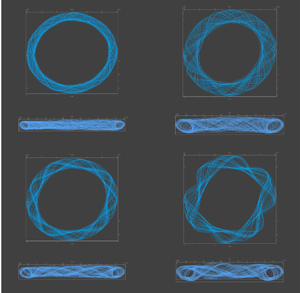
We can track the development of the instability by monitoring the evolution of vorticity or  $Q$ contours (3.2). The shape of a fixed contour $Q = 0.0032 \omega ^{2}$ is shown in figure 9 at four different times. We found empirically that this isosurface showed most of the vortex structure without noticeable noise. A complete time history of the $Q$ field is shown in supplementary movie 2. The initial isosurface (figure 9a) shows two separate sheets, corresponding to a large vortex roll in the bulk fluid and a smaller roll underneath the disk (see supplementary movie 2). When $\omega t \approx 3500$ an instability in the outer vortex becomes visible, signalled by small holes in the larger vortex sheet (figure 9b). Projections of the flow onto a vertical plane indicate that the instability is initiated at the edge of the large vortex roll (supplementary movie 3), rather than in the boundary layer around the disk or along the vertical edges of the disk. The tear in the vortex sheet, centred at approximately $r = 2.3a, z = 0.35h$, corresponds to the region where the ejected flow is entering and reinforcing the vortex roll. Axial symmetry is broken by the instability (figure 9c), and the final oscillating state is a fixed vortex sheet, rotating in the same direction as the disk, with a period of approximately $550 \omega ^{-1}$. There is a precise two-fold symmetry in the sheet, which gives the primary period for the point velocity fields of $275 \omega ^{-1}$.

Figure 9. Isosurface of  $Q = 0.0032\omega ^2$ at ${Re}=800$: (a) $\omega t = 800$; (b) $\omega t = 3520$; (c) $\omega t = 3840$; and (d) $\omega t = 4800$.
4.3. Critical $Re$

The lowest rotation rate for which oscillations develop over the time scale of the simulation ( $\omega t = 17\,500$) corresponds to a Reynolds number ${Re} = 700$. Over the same time range the flow at $Re=600$ remains time invariant (figure 8a,b) with no hint of fluctuations, while at $Re = 800$ it is unsteady before $\omega t = 2500$ (figure 8c,d). An analogy to Taylor–Couette flow suggests that the instability in the vortex sheet (figure 9) is a Hopf bifurcation, leading to an azimuthally periodic flow. Since the subcritical flow ( ${Re} = 600$) is axisymmetric (figure 8a,b), we look for time-dependent perturbations $\delta {\boldsymbol {u}}$ to the mean (base) flow $\overline {\boldsymbol {u}}$:
 \begin{equation} {\boldsymbol{u}}({\boldsymbol{x}}, t) = \overline {\boldsymbol{u}}(r, z) + \delta {\boldsymbol{u}}({\boldsymbol{x}}, t). \end{equation}
However, at  $Re = 700$ the flow is never entirely stationary. Once the initial transient has died out ( $\omega t \sim 2000$), point probes show small (order $10^{-6}$) but very regular fluctuations in the local velocity. These oscillations are too small to be seen on normal scales (figure 8c,d) and we have minimised their effects on the mean flow by averaging over four complete oscillation periods (two rotations), from $\omega t = 2100$ to $\omega t = 3430$.
We have determined the growth rates of the velocity field at different probe positions in the fluid domain (§ 4.3.2). At the two lowest supercritical Reynolds numbers, the growth rate at different probe positions was the same to within the numerical uncertainties (figure 11), with average values of  $0.00074 \omega ^{-1}$ at ${Re} = 700$ and $0.0024 \omega ^{-1}$ at ${Re} = 800$. Since the perturbations are linear in ${Re}$ (§ 4.3.3), by extrapolating to zero growth rate we can estimate the critical Reynolds number as ${Re}_{c} = 655$.
4.3.1. Mean flow
The mean flow at  $Re=700$ separates into three distinct circulation zones, as illustrated by the streamlines in figure 10. Starting from any spatial location a Lagrangian tracer always maps out a path in one of these three zones; no matter how long the streamline, it never crosses into a different zone. In circulation zone I (figure 10a), fluid ejected from the edge of the disk moves towards the bottom of the cylinder, forming a rotating ‘dome’ just underneath the disk. After reaching the bottom of the disk, fluid flows out radially along the base of the container before flowing up the sides (Batchelor flow) to the free surface. Flow lines accumulate towards the centre of the free surface, creating a cyclone flow towards the disk. Flow lines then spiral out from the top of the disk before descending again to the bottom of the container. Circulation zone II (figure 10b) is a vortex ring of radius approximately $2.5 a$ and diameter $\sim a$. Finally, in zone III (figure 10c), the vortex roll is tightly confined under the rotating disk.

Figure 10. Streamlines of the mean flow  $\overline {\boldsymbol {u}}(r,z)$ at ${Re} = 700$. The tracers within each circulation zone are indicated by a different colour: (a) red, zone 1 recirculation; (b) blue, zone 2 vortex roll; (c) white, zone 3 vortex roll underneath the disk.
4.3.2. Velocity probes
Time traces of the axial velocity are shown in figure 11 at 16 different locations, spanning a range of  $r$ and $z$ positions above and below the disk (see figure 2). To make the exponential growth of perturbations clearly visible, the mean flow at each probe position was subtracted. Maxima and minima were detected by comparing the magnitude of $\delta u_z$ at a particular time with values at neighbouring time points. Traces of the other velocity components show similar behaviour, as do probes located in the upper region of the fluid ( $z > 0.6h$).

Figure 11. Axial velocity relative to the mean flow ( $|\delta u_z|$) at the probe positions indicated in figure 2. The plots show the maxima (closed circles) and minima (open circles) in $\delta u_z$. The probes are located at (a) $r = 0.5 a$, (b) $r = a$, (c) $r = 1.5 a$ and (d) $r = 2a$. The vertical positions are indicated by the colour: $z = 0.1 h$ (black); $z = 0.25 h$ (red); $z=0.45 h$ (blue); and $z=0.5 5h$ (green).
The velocity profiles show that perturbations at all the probe points develop with the same frequency and growth rate. This suggests a spatiotemporally periodic flow, with a single global mode growing exponentially in time, similar to the transition from axisymmetric to wavy vortices in Taylor–Couette flow (Davey, Prima & Stuart Reference Davey, Prima and Stuart1968; Jones Reference Jones1985). If we assume a supercritical Hopf bifurcation at  ${Re} \approx 700$, then the flow has an unstable fixed point (mean flow) with a stable limit cycle nearby. We therefore write the perturbation as a single mode (Stuart Reference Stuart1958; Watson Reference Watson1960),
 \begin{equation} \delta {\boldsymbol{u}}({\boldsymbol{x}}, t) = A(t)\delta {\boldsymbol{u}}_0(r,z){\rm e}^{2{\rm i}\theta} + A^\star(t)\delta {\boldsymbol{u}}_0^\star(r,z){\rm e}^{{-}2{\rm i}\theta}, \end{equation}
where  $A(t)$ is the (complex) amplitude; in the linear regime $A = {\rm e}^{-{\rm i}\varOmega t}$. The modes must be even multiples of $\theta$ because of the mirror symmetry in the $r\theta$ plane; figure 8(c,d) shows that the primary instability has a wavenumber of two. The complex field $\delta {\boldsymbol {u}}_0(r,z)$ is a snapshot of the flow field in two $rz$ planes, with an angle of $45^\circ$ between them.
The frequency and growth rate  $\varOmega = (19.0 + 0.74{\rm i})\times 10^{-3} \omega$ were found by fitting data in the linear regime (figure 11) over times $\omega t$ from 6000 to 8000. A single mode grows exponentially and symmetrically about the mean, from the end of the initial transient ( $\omega t \approx 2000$) to the onset of the nonlinear region at $\omega t \approx 10\,000$; eventually the mode stops growing and a stable oscillating state is reached (§ 4.3.4). The rotational period of the vortex roll is $662 \omega ^{-1}$, with two oscillations per complete rotation.
4.3.3. Linear perturbations
A planar projection of the mean flow at  ${Re} = 700$ is shown in figure 12(a). The flow is dominated by two counter-rotating vortex rolls: a large roll in the bulk fluid outside the rotating disk (blue trace in figure 10b) and a smaller roll underneath the disk (white trace in figure 10c). The rolls drive a strong flow from the disk to the container base, where it recirculates to the top of the container (red trace in figure 10a). Regions of high angular velocity in the mean flow (pale blue and red regions) are localised near the disk, in the region between circulation zones II and III, and in the vortex roll underneath the disk.

Figure 12. Maps of the mean flow (a), and perturbation  $\delta {\boldsymbol {u}}$ at $\omega t = 5960$ (b,c). Slice (c) is rotated by $+45^\circ$ with respect to (b). Panel (d) is delayed by seven complete oscillations from panel (b); the length of the lines and the colour scale have been adjusted for the growth of the eigenmode, a factor of 5.55 over this time interval. Flow in the plane $\delta u_r, \delta u_z$ is indicated by arrows, while the perpendicular flow $\delta u_\theta$ is indicated by the colour scale. The arrows indicating the direction of the flow have been clipped from the left side of panel (a) so the variations in colour are more visible.
Spatial variations of the real and imaginary parts of the eigenfunction  $\delta {\boldsymbol {u}}_0(r,z)$ are illustrated in figure 12(b,c). Whereas in the mean flow there are two counter-rotating rolls, the perturbation has corotating vortexes, with an additional small vortex at the base of the separation between circulation zones II and III (figure 10b). The vortexes are fed by the strong shear arising from gradients in the azimuthal velocity, indicated by the changing background colour. In the plane lagging by $45^\circ$ (figure 10c), the small vortex has slipped from the boundary layer and displaced the larger vortex, which is then dissipated by the friction from the nearly stationary outer fluid region ( $r > 3a$). The perturbation to the azimuthal velocity changes sign over the $45\,^\circ$ rotation, as shown by the reversal of the colour maps. The time-periodic vortex shedding can be seen in projections of the axial velocity shown in supplementary movie 4. The large vortex moves towards to the cylinder wall while in the interior it is replaced by a counter rotating vortex.
Figure 12(d) shows the real part of  $\delta {\boldsymbol {u}}_0$ seven oscillations (3.5 rotational periods) later ( $\omega \Delta t = 8280$), with the time lag calculated from the real part of $\varOmega _0$; images of the velocities (arrows and colours) were rescaled based on the imaginary part of $\varOmega _0$. The similarity with figure 12(b) shows that a single mode is evolving in this time range, with a single frequency $\varOmega = (19.0 + 0.74{\rm i})\times 10^{-3} \omega$.
4.3.4. Nonlinear regime
Figure 13 shows axial velocity traces (red lines) from two probes in the boundary layer between zones I and II;  $r = 1.5a$ and $z = 0.1h$ (probe 8) and $z = 0.25h$ (probe 9). The mean velocity over each period was subtracted from the trace and is shown as the blue dotted line. The velocity fluctuations about the time-dependent mean are then well described by the SL equation for the (complex) amplitude (black dotted line),
 \begin{equation} \dot A ={-}{\rm i}\varOmega A - \varGamma A|A^2|, \end{equation}
where  $\varGamma$ is a constant. The amplitude for each probe position was determined fitting a numerical integration of (4.5) to the simulated $\delta u_z$. We used data in the time range $6000 < \omega t < 8000$, where the perturbation to the mean flow is growing exponentially (figure 11). We determine the modulus and phase $A(\omega t = 6000)$ for each probe independently, but the values of $\varOmega$ and $\varGamma$ are the same in both cases. Equation (4.5) captures the saturation of the perturbation and the nonlinear phase shift (approximately ${\rm \pi}$ over the duration of the simulation).

Figure 13. Axial velocity relative to the mean flow ( $|\delta u_z|$) at sample probe positions 8 and 9 ( $r = 1.5a$, $z = 0.1h$ and $r = 1.5a$, $z = 0.25h$). Results from numerical simulations (red) are compared with solutions of the Stuart–Landau (SL) equation (black dots), with $\varOmega = (19.0 + 0.74{\rm i})\times 10^{-3} \omega$ and $\varGamma = (-2.65+3.64{\rm i})\times 10^{-7} \omega$.
For times beyond  $\omega t = 10\,000$, a double minimum appears in the trace for probe 8 (figure 13a), which suggests that higher harmonics are being generated by the nonlinearity. This was confirmed by Fourier transforms of the complete probe trace, which showed an additional peak at twice the frequency of the base signal. If the input signal to the fast Fourier transform was terminated before $\omega t = 10\,000$, there was only a single peak.
The shape of the large vortex roll near the onset of frequency doubling is shown in figure 14. In the linear regime up to times of  $\omega t \approx 9000$, the roll remains circular and flat (figure 14a). As $\omega t$ approaches $10\,000$, the roll expands and a slight waviness in the outline develops (figure 14b). This is not visible at earlier times because the perturbation is too small to significantly impact the overall flow, but by $\omega t = 10\,150$ there are noticeable deviations from flatness and a loss of circular symmetry. There is an abrupt transition in the region $\omega t = 10\,500$, when periodic variations in the overall shape of the vortex develop.

Figure 14. Streamlines showing the outline of the large vortex roll at different times:  ${Re} = 700$; (a) $\omega t = 9100$; (b) $\omega t = 9800$; (c) $\omega t = 10\,150$; (d) $\omega t = 10\,500$. The upper subpanels show the view from the vertical ( $z$) axis, and the lower subpanels the view from the horizontal ( $y$) axis.
4.4. $Re=900\unicode{x2013}1000$

At Reynolds numbers up to 1000, the flow remains organised in coherent vortex rolls, with stable oscillations similar to those at lower Reynolds number. At  ${Re} = 900$ the vortex sheet again just rotates, but with a faster period $440 \omega ^{-1}$. Point velocity probes again show a single frequency in some locations (black line in figure 15a), with two periods per rotation of the vortex, and two frequencies in others (red line) with four periods per rotation. The different frequencies can be understood from the structure of the vorticity (figure 15b); the black and red circles indicate the $(r, z)$ coordinates of the two probes. At ${Re} = 900$ the lobes of vorticity near the free surface have increased in size over those at ${Re} = 800$ and now contribute a significant signal to nearby probe points. It can be seen that the red circle crosses the vorticity sheet eight times in a single rotation, indicting four signals to the probe within one revolution ( $\Delta t = 440 \omega ^{-1}$), matching the observed fluctuations in axial velocity at the outer-upper location (red line in figure 15a). On the other hand, the inner-lower probe (black) is not affected by the upper lobes and only shows two oscillations during a full rotation of the vortex sheet.

Figure 15. Oscillatory flow at  ${Re} =900$ and ${Re} = 1000$. (a) Axial velocity at ${Re}=900$, (b) isosurface at ${Re}=900$, (c) axial velocity at ${Re}=1000$ and (d) isosurface at ${Re}=1000$. The probe locations are at $r=1.5a, z = 0.25h$ and $r=2a, z = 0.45h$; the isosurface contour is $Q = 0.0032 \omega ^2$. The probes lie on the circles of the same colour.
At  ${Re} = 1000$, there are fluctuations in the shape of the vorticity contour as well as rotation ( $\Delta t = 400 \omega ^{-1}$). The dominant signals at the probes are similar to those at the two lower Reynolds numbers, but there are small perturbations from fluctuations in the vortex sheet. This causes additional, less regular, fluctuations in axial velocity.
4.5. Mesh dependence at $Re = 1000$

We have compared the time evolution of the axial velocity at  ${Re} = 1000$ for five different mesh resolutions, all based on the one shown in figure 2(a,b), but at double the resolution shown in the figure. The coarsest mesh (721 920 cells), is denoted ${\mathcal {R}}_{111}$; the other four meshes were various refinements formed by doubling the number of cells in a particular direction: ${\mathcal {R}}_{112}$, ${\mathcal {R}}_{222}$, ${\mathcal {R}}_{114}$ and ${\mathcal {R}}_{224}$.
Figure 16 plots the axial velocity at a single characteristic probe position ( $r=2a, z = 0.45h$) for different mesh resolutions. Figure 16(a,b) compare $u_z(t)$ from the base mesh ( ${\mathcal {R}}_{111}$) and one with double the resolution in the axial direction ( ${\mathcal {R}}_{112}$). Although the flow patterns and oscillation frequencies are quite similar, the point velocities differ by approximately 50 % between the two mesh resolutions. However, further mesh refinement has a much smaller effect on the probe velocities and no visible changes to the flow field. To study finer meshes, without the computational expense required to erase the initial condition, the flow field from the ${\mathcal {R}}_{112}$ mesh at $\omega t = 3000$ was interpolated to more resolved meshes – ${\mathcal {R}}_{222}$, ${\mathcal {R}}_{114}$ and ${\mathcal {R}}_{224}$ – for the comparisons shown in figure 16(c,d). The results figure 16(c) show that the effect of increasing resolution in the $r\theta$ plane is small, while increasing resolution in the $z$ direction leads to a sharpening of the peaks and a small phase shift that accumulates with time. This is not unexpected given the multiple frequencies in the dynamics. Finally, figure 16(d) shows the first period (from $3000 < \omega t < 3200$) including the highest resolution we could calculate ${\mathcal {R}}_{224}$. The different resolutions lead to very similar axial velocities for at least one period and again the in-plane resolution is less important than the axial resolution.

Figure 16. Oscillations of the axial velocity at  ${Re} = 1000$ for mesh resolutions ${\mathcal {R}}_{111}$, ${\mathcal {R}}_{112}$, ${\mathcal {R}}_{222}$, ${\mathcal {R}}_{114}$ and ${\mathcal {R}}_{224}$. The probe is at $r= 2a$, $z = 0.45h$.
In figures 9 and 15, small perturbations can be seen on the surface of the innermost vortex. The four-fold symmetry implies that this is again an artefact of the central square. However, the overall vortex structure is much less sensitive to mesh resolution than in the rotor–stator geometry and the shape of constant  $Q$ contours for more refined meshes remains the same as for ${\mathcal {R}}_{112}$. As a reasonable compromise between accuracy and computational cost we use ${\mathcal {R}}_{112}$ for the simulations up to ${Re} = 5000$.
4.6. Varying disk position and thickness
The flow patterns are very sensitive to disk position. If the rotating disk is moved closer to the base ( $z_{disk} = 0.25h$) the flow is more stable, with a critical Reynolds number in the range $1100 < {Re}_{crit} < 1200$. When ${Re} > 1100$, regular, high frequency ( $\Delta t = 12 \omega ^{-1}$) oscillations emerge after some initial transients (figure 17a). The fast oscillations are caused by the development of spiral waves in the bulk fluid outside the rotating disk (figure 17b). With the disk in the central position ( $z_{disk} = 0.5h$), spiral waves are never observed (figures 8–15), but here the additional friction between the spinning disk and the container base provokes an additional instability in the vortex sheet; the sequence can be followed in figure 17(c). Initially ( $\omega t \approx 120$) a circular vortex forms outside the disk, indicated by the middle ring. This vortex ring develops instabilities around its exterior around $\omega t \approx 240$, which break up into six pairs of spiral vortexes ( $\omega t \approx 360$). Each pair is composed of a large interior roll and a smaller exterior one. The six spiral pairs coalesce quickly ( $\omega t \approx 480$) into three larger pairs, which becomes the stable structure (figure 17b). We observed similar flow patterns up to ${Re} = 2000$.

Figure 17. Oscillatory flow at  ${Re} = 1200$ with the central plane of the rotating disk located at the quarter height $z_{disk} =0.25h$. (a) Axial velocity at a single radial position $r=2a$, indicated by the red circle. The circle is coplanar with the central plane of the disk ( $z = 0.25h$). The three probes are near the base of the container ( $z = 0.1h$), coplanar with the disk ( $z=0.25h$) and in the fluid above the disk ( $z = 0.45h$). (b) Isosurface of $Q = 0.0032 \omega ^2$ at $\omega t = 4800$, showing three pairs of spiral vortexes. (c) Isosurfaces of $Q = 0.0032 \omega ^2$ at $\omega t = 120, 240, 360, 480$.
If the disk is shifted upwards, towards the free surface, the reduced resistance to rotational flow near the free surface (compared with a no-slip boundary) allows for unstable flows at lower  ${Re}$. The critical Reynolds number decreases, and with $z_{disk} = 0.75h$ the flow becomes unstable in the range $100 < {Re} < 200$. In this case there is a symmetry breaking in the $rz$ plane, with an upward flow on one side and a downward flow on the other. Images of the flow are shown in figure 18 at a Reynolds number ${Re} = 300$. Over time the axial flow oscillates back and forth with a period of approximately $\Delta t = 360 \omega ^{-1}$. The four images show the flow switching back and forth at intervals of approximately $\Delta t/4$. The uniform flow towards the disk suggested by the similarity solution does not occur here.

Figure 18. Oscillatory flow at  ${Re} = 300$ with the central plane of the rotating disk located at the three-quarter height, $z_{disk}=0.75h$; the flow field near the rotating disk is projected on the $yz$ plane. Flow fields are shown at four successive times: (a) $\omega t = 1200$; (b) $\omega t = 1290$; (c) $\omega t = 1380$; and (d) $\omega t = 1470$. The colour scale indicates the magnitude of the in-plane flow field, $u_{yz} = (u_y^2+u_z^2)^{1/2}$.
We did not find significant variations with a centrally placed disk of half the original thickness ( $d = 0.025h$). The instability develops within the same range of ${Re}$ and the flow patterns are similar to the thicker ( $0.05h$) disk. This is consistent with an instability in the vortex roll outside the disk (§ 4.3), rather than being generated at the edge of the disk.
4.7. Transition to turbulence: $Re = 1200\unicode{x2013}5000$

With the disk centrally positioned ( $z_{disk} = 0.5h$) the flow below ${Re} = 2000$ is characterised by rotation of the vortex sheet, but the mirror symmetry present in lower ${Re}$ flows is lost. The shape of a fixed $Q$ contour is no longer constant, but the oscillations first observed at ${Re} = 1000$ grow in magnitude and complexity. In figure 19 the velocity field has been projected onto an ( $rz$) plane. The higher velocity regions (light blue to red) envelope more or less symmetric vortex rolls, but these rolls change shape and spawn new vortexes as the primary vortex sheet rotates. The flow becomes more asymmetric as ${Re}$ increases and the size of the rolls decreases noticeably at ${Re} = 2000$. Up to ${Re} = 2000$ the vortex core is almost entirely contained within a single rotating sheet, with only a few isolated vortex blobs. But, by ${Re} = 3000$, there is a sharp increase in the axial velocity fluctuations and the flow becomes turbulent; there is no longer any structure to the vorticity, just blobs of different sizes and shapes. Simulations at ${Re} = 5000$ suggest that the flow has become fully turbulent. For comparison, the experiment described by Gregory & Riddiford (Reference Gregory and Riddiford1956) was at ${Re} \sim 10\,000$.

Figure 19. Flow fields at higher Reynolds numbers: (a)  ${Re} = 1200$; (b) ${Re} = 1500$; (c) ${Re} = 2000$; (d) ${Re} = 3000$; (e) ${Re} = 5000$. The colour scale indicates the magnitude of the in-plane flow field, $u_{yz} = \sqrt {u_y^2+u_z^2}$.
5. Conclusions
We have simulated rotating flows in rotor–stator and spinning disk geometries using direct numerical simulations with finite-volume discretisation. Our results for rotor–stator flows (§ 3) reproduce the key results from previous spectral simulations (Serre et al. Reference Serre, Tuliszka-Sznitko and Bontoux2004): a critical Reynolds number  ${Re}_{crit} \approx 11\,500$, with a periodic flow formed by rotating spiral vortexes. Our finest meshes reproduced the correct number of spirals at ${Re} = 13\,200$, but we were unable to demonstrate that the mesh was fully converged. The finest mesh utilised $12 \times 10^6$ cells, as opposed to approximately 150 000 cells in a fully resolved spectral simulation. A mixed discretisation, using finite-volume cells in the $rz$ plane and a spectral decomposition in the axial direction, may prove to be an efficient solution in more general axisymmetric geometries. Among other things, it would avoid the artefacts in the present work associated with merging Cartesian and polar meshes.
New results were obtained for a finite-size disk rotating in a larger volume of fluid (§ 4). The simulations include a free surface as the top boundary condition, which mimics the typical experimental set-up for surface reaction rate measurements. At low Reynolds number ( ${Re} \sim 100$) the flow is time independent, with the vorticity confined in symmetric doughnut-shaped rolls. This flow is unstable to an imbalance in centrifugal and pressure forces, and mirror symmetry is broken at Reynolds numbers in excess of 100. However, the double vortex flow (figure 7g,h) remains stable and time invariant up to Reynolds numbers around 700. At that point, azimuthal symmetry is broken (figure 6c,d) by a Hopf bifurcation, and a two-fold symmetric vortex sheet is formed (figures 9 and 15). The outer vortex develops periodic oscillations, similar to the rolls in a wavy Taylor–Couette flow, but the overall vorticity envelope simply rotates until a Reynolds number of 1000 is reached, when small fluctuations develop. The amplitude increases with increasing Reynolds number and after ${Re} = 1200$, the mirror symmetry characterising the slower flows is lost. Velocity fluctuations become more chaotic until the onset of a turbulent flow in the range $3000 < {Re} < 5000$. Reynolds numbers in laboratory experiments are in the same range, ${Re} \approx 10\,000$ (Gregory & Riddiford Reference Gregory and Riddiford1956).
Time varying flows are sensitive to the disk position. If it is shifted below the central plane ( $z_{disk} = 0.25h$), spiral vortexes develop outside of the spinning disk near the base of the cylinder (figure 17). On the other hand, moving the disk upwards ( $z_{disk} = 0.75h$) breaks the mirror symmetry in the $r \theta$ plane. In this case a very large vortex flow develops on top of the disk, which dominates the $rz$ velocity. The direction of the vortex flow switches periodically in time ( $\Delta t \approx 360 \omega ^{-1}$).
Supplementary material and movies
Supplementary material and movies are available at https://doi.org/10.1017/jfm.2022.566.
Acknowledgements
Results from finite-volume simulations were generated with the OpenFOAM-v1912 tool kit, http://www.openfoam.com/. Images of the flow field were created in ParaView, https://www.paraview.org/.
Funding
This material is based upon work supported by the US Department of Energy, Office of Science, Office of Basic Energy Sciences, Chemical Sciences, Geosciences and Biosciences Division under award number DE-SC0018676.
Declaration of interests
The authors report no conflict of interest.


 Open access