


1. Introduction
Doubly diffusive fingering convection has been the subject of many studies over the past few decades owing to its relevance to natural processes such as oceanography, geophysics and astrophysics (Stern Reference Stern1969; Turner Reference Turner1985; Schmitt Reference Schmitt1994; Garaud Reference Garaud2018). Fingering convection occurs when two density-changing components with different diffusivities are stratified in a fluid so that the slower diffusing component produces an unstable vertical gradient and the faster diffusing component produces a stronger opposite gradient, resulting in an overall decrease of the fluid density in the upward direction. This type of set-up is unstable to infinitesimal disturbances displacing the fluid vertically: because the stabilizing faster diffusing component remains more horizontally homogeneous than the destabilizing slower diffusing one, a pattern of buoyancy anomalies emerges with a characteristic spatial scale, leading, close to marginality, to the growth of alternatively rising and sinking columnar structures, named ‘salt fingers’, characterized by deficiency and abundance of the slower diffusing component (Radko Reference Radko2013).
Fingering convection is fuelled by the release of potential energy stored in the unstably stratified slower diffusing component, and it generates an up-gradient transport of buoyancy. Even in the nonlinear regime of fully developed convection, a necessary condition for this to occur is  $1< R_{\rho }< Le$ (Middleton & Taylor Reference Middleton and Taylor2020), where the density ratio $R_{\rho }$ measures the relative contribution to the buoyancy of the two diffusers and $Le$ is the Lewis number (see § 2.1 for the definitions).
For  $R_{\rho }\to Le$, the system is close to be marginally unstable and the finger structures appear as tall, narrow convection cells, spanning the entire height of the domain, and circulating in a laminar flow (Linden Reference Linden1973; Turner Reference Turner1973). Most of the work on quantifying and explaining the fluxes carried by fingering convection is, to this day, anchored to the depiction of salt fingers as nearly stationary, tall and narrow convection cells (see, e.g. Schmitt Reference Schmitt1979; Radko & Stern Reference Radko and Stern2000; Pringle & Glass Reference Pringle and Glass2002; Yang, Verzicco & Lohse Reference Yang, Verzicco and Lohse2016). However, in the oceanographically relevant regime with low values of $R_{\rho }$ and high Rayleigh numbers, fingering convection becomes vigorous, and further instabilities affect the elongated convection cells (Holyer Reference Holyer1981, Reference Holyer1984, Reference Holyer1985; Stern & Simeonov Reference Stern and Simeonov2005). As first recognized by Shen (Reference Shen1995), far beyond marginality and at low enough density ratio, these instabilities result in the formation of buoyancy-carrying structures of much more limited vertical extent that appear as blobs having an approximate 1-to-1 aspect ratio (Radko Reference Radko2008; von Hardenberg & Paparella Reference von Hardenberg and Paparella2010; Traxler et al. Reference Traxler, Stellmach, Garaud, Radko and Brummell2011).
These blobs are localized regions characterized by a severe buoyancy excess or deficiency compared with that of the surrounding fluid. They are not stationary, but move upward or downward according to their own buoyancy anomaly, while their motion is continuously perturbed by the interaction with nearby blobs (von Hardenberg & Paparella Reference von Hardenberg and Paparella2010). Their presence has been linked to a large-scale instability that occurs at very low density ratios, which gives rise to a layered, staircase-like appearance of the horizontally averaged density profile (Paparella & von Hardenberg Reference Paparella and von Hardenberg2012, Reference Paparella and von Hardenberg2014; Coclite, Paparella & Pellegrino Reference Coclite, Paparella and Pellegrino2018).
In this paper, we shall focus on the non-staircase-forming regime. In this regime, far from the boundaries, the horizontally averaged density and density-changing components reach a stationary state characterized by constant vertical gradients. We track Lagrangian particles to investigate the degree of vertical coherency of the buoyancy-carrying structures, which parts of the fluid carry most of the up-gradient flux and the conditions that allow for a coherent vertical motion of such structures. The goal of this study is solely that of illustrating the Lagrangian properties of fingering convection, and not of modelling any specific, naturally occurring phenomenon.
The rest of the paper is organized as follows: § 2 defines the problem and describes the numerical simulations; § 3 reports the results of the Lagrangian analysis; § 4 proposes a view of fingering convection based on the coherent vertical motion of the blobs, which perform the dual role of carriers of the up-gradient flux and of prime motors of all of the convective motions.
2. Equations and numerical simulations
2.1. Equations of motion
Throughout this study, we designate the two density-changing components to be ‘salinity’ and ‘temperature’ for respectively the least and the most diffusing components. We consider a layer of fluid with thickness  $d$ enclosed between two parallel infinite walls that are maintained at constant temperature and salinity. The temperature and salinity differences between the top and the bottom walls are assumed to be ${\rm \Delta} T$ and ${\rm \Delta} S$, respectively. The control parameters of the problem are the Prandtl, Lewis, thermal and haline Rayleigh numbers, defined as
 \begin{equation} Pr = \frac{\nu}{\kappa_T},\quad Le = \frac{\kappa_T}{\kappa_S},\quad R_T = \frac{g\alpha{\rm \Delta} T d^3}{\nu \kappa_T},\quad R_S = \frac{g\beta{\rm \Delta} S d^3}{\nu \kappa_S}, \end{equation}
where  $\nu$ is the kinematic viscosity, $\kappa _T$ is the thermal diffusivity, $g$ is the acceleration due to gravity, and $\alpha$ and $\beta$ are the thermal and haline linear expansion coefficients. From these, the density ratio $R_{\rho }$ is defined as
 \begin{equation} R_{\rho}=Le\frac{R_T}{R_S}. \end{equation}
The fluid motion is governed by the Boussinesq equations that take the following dimensionless form (Paparella & von Hardenberg Reference Paparella and von Hardenberg2012):
 \begin{gather} \boldsymbol{\nabla}\boldsymbol{\cdot}\boldsymbol{u} = 0, \end{gather}
 \begin{gather}\frac{\partial\boldsymbol{u}}{\partial t}+(\boldsymbol{u}\boldsymbol{\cdot}\boldsymbol{\nabla}) \boldsymbol{u} ={-}\boldsymbol{\nabla} p +Pr Le\left(\nabla^2\boldsymbol{u}+R_SB \hat{\boldsymbol{z}}\right), \end{gather}
 \begin{gather}\frac{\partial T}{\partial t}+(\boldsymbol{u}\boldsymbol{\cdot}\boldsymbol{\nabla})T = Le\nabla^2 T, \end{gather}
 \begin{gather}\frac{\partial S}{\partial t}+(\boldsymbol{u}\boldsymbol{\cdot}\boldsymbol{\nabla})S = \nabla^2 S. \end{gather}
In this paper, we consider the two-dimensional case, thus  $\boldsymbol {u}=(u, w)$ is the velocity field of the fluid that occupies the dimensionless domain $\boldsymbol {x}=(x,z)\in [0, L_x]\times [0, 1]$; $p$ is the pressure; $T$ and $S$ are the temperature and salinity fields, whose value ranges from 0 at the bottom wall to 1 at the top wall; $B= R_{\rho }T-S$ is the buoyancy field and $\hat {\boldsymbol {z}}$ is the upward unit vector. The vorticity field associated with $\boldsymbol {u}$ is defined to be $\omega :=\partial _{z}u-\partial _{x}w$. All variable fields are assumed to be laterally periodic. Free-slip conditions are enforced on momentum at both walls. The stationary base state of (2.3a)–(2.3d) reads
 \begin{equation} \left(\boldsymbol{u}_b, T_b, S_b\right) = \left((0, 0), z, z\right). \end{equation}
 The solutions of (2.3a)–(2.3d) develop thermal and haline boundary layers near the top and bottom walls. In the interior, depending on the value of the parameters in (2.1a–d), the horizontally averaged temperature and salinity profiles may either form a slowly evolving staircase-like profile or reach a statistically steady state characterized by constant vertical gradients  $G_T$ and $G_S$, with $G_S < G_T < 1$. In this case, the strength of the convection is best quantified by the local density ratio $R_{\rho \ {loc}}$, defined as
 \begin{equation} R_{\rho\ {loc}} = \frac{G_T}{G_S}R_{\rho}. \end{equation}
 We define the anomaly of a scalar field  $({\cdot })$ with respect to its horizontal average as
 \begin{equation} ({\cdot})':= ({\cdot})-\overline{({\cdot})}:=({\cdot})- \frac{1}{L_x} \int_{0}^{L_x} ({\cdot})\,\mathrm{d}\kern0.7pt x, \end{equation}
in which  $\overline {({\cdot })}$ is the horizontal average of $({\cdot })$. The buoyancy anomaly is thus
 \begin{equation} B^\prime = R_{\rho}T^\prime-S^\prime. \end{equation}
Because  $\bar {w}=0$, only the buoyancy anomaly flux $B^\prime w$ contributes to the total advective buoyancy flux across any horizontal section of the domain.
We define a Lagrangian particle as a geometric point whose velocity coincides with that of the fluid. That is, a Lagrangian particle sweeps a curve  $\boldsymbol {x}_0\mapsto \boldsymbol {x}(\boldsymbol {x}_0; t)$ uniquely defined by
 \begin{equation} \frac{{\rm d}\kern0.7pt \boldsymbol{x}(t)}{{\rm d} t} = \boldsymbol{u}(\boldsymbol{x}(t), t),\quad \boldsymbol{x}(\boldsymbol{x}_0; 0) = \boldsymbol{x}_0, \end{equation}
where  $\boldsymbol {u}(\boldsymbol {x}, t)$ is the fluid velocity at the current particle position (as given by (2.3a)–(2.3d)). We designate a Lagrangian particle's buoyancy, salinity and temperature anomalies to be the same as those of the fluid's at the particle's current location.
2.2. Numerical set-up
Equations (2.3a)–(2.3d), recast in the vorticity-streamfunction formulation, were solved numerically with a Galerkin pseudo-spectral code. The numerical method uses the Fourier basis in the horizontal direction and the sine basis in the vertical. Time evolution is implemented through a third-order Adams–Bashforth scheme. The initial condition consists of the conductive solution (2.4) with a small white noise perturbation added to the salinity field. We monitor the temperature and salinity fluxes computed in the bulk of the domain (defined as the middle third of it) and at the boundary of the domain. During the initial transient, the fluxes in the bulk are larger (in absolute value) than the fluxes at the boundary. When the transient is over and the boundary layers become fully established, the fluxes in the bulk and at the boundary match each other, and remain nearly constant in time. To check that no thermohaline staircases are formed, we extend the Eulerian part of the simulations for at least five times the duration of the initial transient (see supplementary figure S7 available at https://doi.org/10.1017/jfm.2023.311). During this time, we check that a statistically steady state is maintained where the horizontally averaged temperature, salinity and buoyancy, far from the boundaries, keep a constant vertical gradient. We then seed at uniformly random positions within the entire computational domain a number of Lagrangian particles equal to the number of Eulerian grid points. The time step ( ${\rm \Delta} t$) used in the simulations was chosen to maintain a Courant–Friedrichs–Lewy (CFL) number (based on the vertical velocity) of approximately $0.2$. The Lagrangian data are saved every 100 time steps. Each Lagrangian simulation lasts for a time interval in which a particle travelling at the CFL speed would cover five times the height of the computational domain. The motion of the Lagrangian particles is tracked with the same time integrator used for the Eulerian part. The velocity of the particles is computed by taking the derivative of a bicubic interpolator of the streamfunction. This method ensures the divergenceless of the interpolated velocity field. The parameters of the simulations used in this study are presented in table 1. We consider two groups of simulations: one where the density ratio is fixed to $R_\rho =1.2$ and the haline Rayleigh number is $R_S=10^{12},\ 3.16\times 10^{12},\ 10^{13},\ 3.16\times 10^{13},\ 10^{14}$, and one in which the haline Rayleigh number is fixed to $R_S=10^{12}$ and the density ratio is $R_\rho =2.8, 2.4, 2.0, 1.6, 1.2$. In all simulations, we fixed $Pr =10$ and $Le = 3$. The simulations with fixed density ratio explore a regime very far from marginality, where fingering convection is quite vigorous and is characterized by large fluxes and fast-moving blobs, but not vigorous enough to lead to staircase formation. The simulations with fixed haline Rayleigh number are intended to investigate whether the blob-dominated regime breaks down when the density ratio approaches the marginally stable value $R_\rho =Le$.
Table 1. Parameters of simulation runs: haline ( $R_S$) and thermal ( $R_T$) Rayleigh numbers, domain width ( $L_x$), mesh size ( $N_x\times N_z$), time step ( ${\rm \Delta} t$) and local density ratio $R_{\rho \ {loc}}$ at equilibrium. We fixed $Pr =10$ and $Le = 3$ in all simulation runs. Note that the simulations with $R_S=10^{12}$ have a density ratio $R_\rho =2.8, 2.4, 2.0, 1.6, 1.2$, from top to bottom; the other simulations all have $R_\rho =1.2$.

2.3. Lagrangian legs and leg statistics
We partitioned the trajectory of every Lagrangian particle into a set of shorter fragments that we refer to as the legs. We define a leg to be a maximal section of a trajectory with strictly increasing or decreasing elevation, i.e. the  $z$-coordinate along a leg is monotone. The monotonicity alternates between adjacent legs. For every leg, $l$, we define the signed leg length, $\zeta$ of $l$, to be the difference between $z$-coordinates of its terminal and initial points. Thus, legs with a positive length correspond to up-going particles, and those with a negative length correspond to down-going particles. In the supplementary figure S1, we present a visual illustration of a particle trajectory and of the legs of which it is made.
We define a leg's properties (buoyancy anomaly, vertical velocity, flux of buoyancy anomaly, etc.) to be the mean of those quantities along the leg. Specifically, if a leg begins at time  $t_s$, ends at time $t_e$ and describes the curve $\boldsymbol {x}$, then we define its property $g_l$ as
 \begin{equation} g_l := \frac{1}{t_e - t_s} \int_{t_s}^{t_e} g(\boldsymbol{x}(t), t)\,{\rm d} t\quad \mbox{where}\ g\in\{B^\prime, w, B^\prime w,\ldots\}. \end{equation}
 We include in the statistics only legs that lie entirely within the central region  $0.2\leq z\leq 0.8$. In this portion of the domain, the horizontally averaged temperature and salinity profiles are linear in all of the simulations that we performed (table 1). Thus, we have excluded from the leg-based statistics the contribution of the boundary layers.
Leg lengths are compared with the characteristic horizontal size of the doubly diffusive blobs moving in the fluid. A useful quantification of such size is given by the following integral scale (Paparella & von Hardenberg Reference Paparella and von Hardenberg2012):
 \begin{align} l_{\omega} := {\rm \pi} \left\langle \frac{\displaystyle\sum_{n=1}^{\infty}k_n^{{-}1} |\hat{\omega}|^2(z, k_n)}{\displaystyle\sum_{n=1}^{\infty}|\hat{\omega}|^2(z, k_n)}\right\rangle_{{z}}, \end{align}
where  $k_n=2{\rm \pi} n/L_x$ is the horizontal wavenumber, $|\hat {\omega }|^2$ is the power spectral density of the vorticity field (where it is intended that the Fourier transform is only taken along the horizontal direction), and the angular bracket denotes a time and vertical average in the interval $0.2\leq z\leq 0.8$.
3. Leg statistics
Table 2 summarizes the main statistics of the Lagrangian legs for the set of simulations with  $R_\rho =1.2$ and $R_S=10^{12},\ldots,10^{14}$. A large majority of legs has a length shorter than the typical size $l_\omega$ of a doubly diffusive blob. The fraction of legs which is longer than a blob shows a slight increase with increasing Rayleigh number $R_S$ (and thus with decreasing local density ratio $R_{\rho \ {loc}}$). For all cases considered in table 2, only 5 % of the legs is longer than $\sim$4.5 blob lengths and only 1 % of the legs is longer than $\sim$10 blob sizes. The exact values of the length of the 95th and 99th percentiles show a substantial decrease with increasing $R_S$ when measured in units of the domain height, and a nearly negligible increase when measured in units of the blob size $l_\omega$.
Table 2. For each simulation having density ratio  $R_\rho =1.2$, we report (top to bottom): the haline Rayleigh number; the number of legs lying in $0.2\le z \le 0.8$; the blob size $l_\omega$; the fraction of legs with length smaller than $l_\omega$; and the 95th and 99th percentiles of the leg length distribution (values in parentheses are in units of $l_\omega$).

Table 3 shows the same statistics for the set of simulations with  $R_S=10^{12}$ and $R_\rho =1.2,\ldots,2.8$. The length in units of $l_\omega$ of the 95th and 99th percentiles shows a substantial increase with increasing $R_\rho$, except at the highest density ratio $R_\rho =2.8$, where it drops back to values similar to those attained at $R_\rho =1.2$.
Table 3. For each simulation having haline Rayleigh number  $R_S=10^{12}$, we report (top to bottom): the density ratio $R_\rho$; the number of legs lying in $0.2\le z \le 0.8$; the blob size $l_\omega$; the fraction of legs with length smaller than $l_\omega$; and the 95th and 99th percentiles of the leg length distribution (values in parentheses are in units of $l_\omega$).

In the following, ‘long legs’ are those with length  ${\gtrsim }5 l_\omega$ and ‘short legs’ those with length ${\lesssim }l_\omega$.
3.1. Link between leg length and buoyancy anomaly, vertical velocity, buoyancy flux
Figure 1 shows the bivariate frequency of leg length  $\zeta$ and of leg buoyancy anomaly $B^\prime _l$, normalized with respect to the number of legs, for the simulations with $R_S=10^{12}$ and $R_S=10^{14}$. It also shows the conditional expectation $E(B^\prime _l\,|\,\zeta )$, namely the average buoyancy anomaly of legs having length $\zeta$. (Similar figures for the remaining simulations are presented in the supplementary materials.)

Figure 1. Bivariate frequency (normalized with respect to the number of legs, see table 2) of leg buoyancy anomaly ( $B^\prime _l$) and leg length ( $\zeta$) for (a) $R_S=10^{12}$, (b) $R_S= 10^{14}$. The red curve shows the conditional expectation $E(B^\prime _l\,|\,\zeta )$.
It is immediately evident that long legs do not occur unless their buoyancy anomaly is close to an optimum value (approximately  ${\pm }0.8$ for $R_S=10^{12}$ and ${\pm }0.35$ for $R_S=10^{14}$). Short legs, instead, may carry a wide range of buoyancy anomalies. Extreme buoyancy anomaly values are always associated with short legs, but these extreme events are rare: the conditional expectation $E(B^\prime _l\,|\,\zeta )$ reveals that short legs are, on average, associated with small buoyancy anomalies. The sign of the buoyancy anomaly generally agrees with that of the leg length. Thus, as expected, Lagrangian particles associated with positive buoyancy anomaly move upward, and those associated with negative buoyancy anomaly move downward. Given the overall stratification of a fingering convection set-up (heavier fluid underneath lighter fluid), this is the signature of the up-gradient density transport, which is the defining characteristic of doubly diffusive convection. However, short legs make an exception: for legs having length closer to zero, the sign of the buoyancy anomaly is, on average, the opposite of that of the leg length (see the wiggle in $E(B^\prime _l\,|\,\zeta )$ near $\zeta =0$), suggesting that short legs, on average, are associated with a down-gradient flux.
Figure 2 shows the bivariate frequency of leg length  $\zeta$ and of leg vertical velocity $w_l$. Just as for buoyancy anomaly, long legs are associated with a relatively narrow band of vertical velocities (either positive, for up-going legs, or negative, for down-going ones). Short legs, instead, exhibit a wider range of vertical velocities, including velocities exceeding those of the long legs. However, on average, a shorter leg will move slower.

Figure 2. Bivariate frequency (normalized with respect to the number of legs, see table 2) of leg vertical velocity ( $w_l$) and leg length ( $\zeta$) for (a) $R_S=10^{12}$, (b) $R_S= 10^{14}$. The red curve shows the conditional expectation $E(w_l\,|\,\zeta )$.
Figure 3 shows the bivariate frequency of leg length  $\zeta$ and of leg advective buoyancy flux $(B^\prime w)_l$. Once again, we find that long legs are associated with a relatively narrow band of advective buoyancy fluxes. Furthermore, long legs always carry positive (up-gradient) fluxes, whereas short legs may carry both positive and negative (down-gradient) fluxes.

Figure 3. Bivariate frequency (normalized with respect to the number of legs, see table 2) of leg advective buoyancy flux ( $(B^\prime w)_l$) and leg length ( $\zeta$) for (a) $R_S=10^{12}$, (b) $R_S= 10^{14}$. The red curve shows the conditional expectation $E((B^\prime w)_l\,|\,\zeta )$.
Figures 4 and 5 show all three bivariate distributions ( $\zeta$ versus $B^\prime _l$, $w_l$ and $(B^\prime w)_l$) for respectively the simulations with $R_\rho =2.0$ and $R_\rho =2.8$, and $R_S=10^{12}$ (those for the other density ratios are in the supplementary materials). Even at high density ratios, the Lagrangian dynamics appears to show the same qualitative properties as in the runs at $R_\rho =1.2$. At $R_\rho =2.0$, and for long legs, the fluctuations around the conditional expectation $E(B^\prime _l\,|\,\zeta )$ are the smallest compared with any other parameter set that we examined. However, at $R_\rho =2.8$, the spread around the average is much larger.

Figure 4. Bivariate frequency (normalized with respect to the number of legs, see table 3) of (a) leg buoyancy anomaly ( $B^\prime _l$), (b) leg vertical velocity ( $w_l$), (c) leg advective buoyancy flux ( $(B^\prime w)_l$) and leg length ( $\zeta$) for $R_S=10^{12}$, $R_{\rho }=2.0$ . The red curve shows the conditional expectations $E(B^\prime _l\,|\,\zeta )$, $E(w_l\,|\,\zeta )$, $E((B^\prime w)_l\,|\,\zeta )$.

Figure 5. As in figure 4, but for  $R_S=10^{12}$, $R_{\rho }=2.8$.
We approximate the conditional expected flux at a given leg with the following expression:
 \begin{equation} E\left((B^\prime w)_l\,|\,|\zeta|\right) \approx F_{max}\left(1-\exp\left({-\frac{|\zeta|}{\zeta_0}}\right)\right), \end{equation}
where the free parameters  $\zeta _0$ and $F_{max}$ are least-squares fitted to the simulation data. The value of $F_{max}$ estimates the flux that would be associated with legs of formally infinite length. In figure 6, we compare the conditional flux $E((B^\prime w)_l\,|\,|\zeta |)$ of all the simulations of table 1 by normalizing it with respect to $F_{max}$, and plotting it as a function of $|\zeta |/l_\omega$, which is the unsigned leg length expressed in units of the blob size of each simulation. The results of the simulations with $R_\rho =1.2$ collapse almost perfectly on top of each other. The flux reaches half of its maximum for leg lengths of approximately 10 times the size of a blob, and saturates at $|\zeta |/l_\omega \approx 40$. For $R_S=10^{12}$, the curves become progressively less steep as the density ratio $R_\rho$ is increased, and at high density ratio, saturation is not attained. The simulation with the highest density ratio $R_\rho =2.8$, however, breaks the trend, and saturates more quickly than any other.

Figure 6. Normalized conditional expectation  $E((B^\prime w)_l\,|\,|\zeta |)/F_{max}$ as a function of the leg length in units of the blob size $|\zeta |/l_\omega$ for all the simulations in table 1. Curves labelled with the density ratio $R_\rho$ refer to simulations with $R_S=10^{12}$. Curves labelled with the haline Rayleigh number $R_S$ refer to simulations with $R_\rho =1.2$.
3.2. What carries the flux
The bivariate distributions presented above show that all long legs tend to be associated with roughly the same values of buoyancy anomaly ( $B_l^\prime$), vertical velocity ( $w_l$) and up-gradient advective buoyancy flux ( $(B^\prime w)_l$). However, they do not immediately reveal how the flux is partitioned among legs of different lengths. In other words, we still need to ascertain whether most of the flux in fingering convection is carried by portions of the fluid that coherently travel in the same direction, or, instead, the flux is mostly determined by the jittery, incoherent motion revealed by the large amount of short legs. To answer this question, we introduce the cumulative flux fraction, $C_F(|\zeta |)$, which is the fraction of the total flux associated with legs having length up to $|\zeta |$:
 \begin{equation} C_F\left(|\zeta|\right) := \frac{\displaystyle\int_0^{|\zeta|} \int_{-\infty}^{+\infty} p(\xi, F) F\,\mathrm{d}F\,\mathrm{d}\xi}{\displaystyle \int_{0}^{\infty}\int_{-\infty}^{+\infty} p(|\zeta|, F) F\,\mathrm{d}F\,\mathrm{d}|\zeta|}, \end{equation}
where  $p$ is the joint probability distribution of unsigned leg length $|\zeta |$ and leg advective buoyancy flux $F=(B^\prime w)_l$.
The cumulative flux fraction is shown in figure 7 for the simulations with  $R_S=10^{12}$ and $R_S=10^{14}$ (see supplementary materials for the others). At $R_S=10^{12}$, the cumulative flux is negative (down-gradient) up to lengths $\sim$1.6 times the blob size $l_\omega$. At $R_S=10^{14}$, this value increases to $\sim$2.5 $l_\omega$. The very abundant short legs carry a down-gradient flux which reaches 12 % of the total flux at $R_S=10^{12}$ and 21 % of it at $R_S=10^{14}$ (minima of the cumulative flux fraction). At $R_S=10^{12}$, 50 % of the up-gradient flux is carried by legs longer than $\sim$4.5 $l_\omega$, and this increases to 60 % at $R_S=10^{14}$. Thus, the bulk of the up-gradient flux is carried by legs substantially longer than the size of a blob. Even though these long legs are fewer in number (the distribution of leg lengths is shown in red in figure 7), their positive flux is sufficient to overcome the negative one carried by the much more abundant short legs.

Figure 7. Cumulative flux fraction (green line) as a function of the leg length (left axis). Probability density function of the leg length (red line, right axis, log scale). (a) Simulation with  $R_S=10^{12}$, (b) simulation with $R_S=10^{14}$.
In figure 8, we show the cumulative flux fraction and the leg length probability density function for the simulations with  $R_S=10^{12}$ and $R_\rho =1.2,\,2.0,\,2.8$. In this case, on the horizontal axis, we show the leg length as a fraction of the domain height. As the density ratio increases, the down-gradient flux carried by short legs becomes negligibly small. This result suggests that down-gradient fluxes are the result of mechanical mixing operated by fast-moving blobs: vertical velocities dramatically decline (figures 2(a), 4(b), 5(b)) with increasing density ratio, and with them, the ability of the blobs to stir the surrounding fluid. Correspondingly, long legs become longer and more abundant (table 3) because blobs are less disturbed by nearby ones as they move vertically. However, any trend associated with lengthening leg lengths breaks down when the density ratio becomes close enough to the marginal stability threshold $R_\rho =Le$ (recall that here we are using $Le=3$). At $R_\rho =2.8$, the exponential tail of the leg length distribution becomes steeper than at $R_\rho =1.2$; very long legs become rarer (table 3); the normalized conditional expectation $E((B^\prime w)_l\,|\,|\zeta |) / F_{max}$ becomes steeper (figure 6). Considering that at marginal stability, the fluid would be at rest, and legs would have zero length, the breakdown of the trends appears to be a natural consequence of the continuous dependence of the flow statistics on the density ratio.

Figure 8. As in figure 7(a), but for the simulations with  $R_S=10^{12}$ and density ratio $R_\rho =1.2$ (solid lines), $R_\rho =2.0$ (dashed lines), and $R_\rho =2.8$ (dotted lines). Note that the horizontal axis now expresses the leg lengths as a fraction of the domain height, rather than in blob size units.
4. Discussion and conclusions
Our findings reveal that, in the non staircase-forming regime, the up-gradient fluxes of fingering convection are associated with coherent vertical motions of fluid parcels that span lengths substantially longer than the size of the buoyancy-carrying structures (the doubly diffusive blobs), but much shorter than the vertical height of the domain. Therefore, the picture of salt fingers as ‘tall convection cells’ appears to be inappropriate to describe this regime. Instead, a depiction of salt fingers as Lagrangian, buoyancy-carrying, coherent structures is, in our opinion, much more satisfactory. The notion that vigorous fingering convection is dominated by vertically moving blobs dates back at least to Shen (Reference Shen1995). However, this finding has rarely been taken as the basis of a description of the large-scale phenomenology of fingering convection, or of a theory of fluxes (the works by Radko (Reference Radko2008), von Hardenberg & Paparella (Reference von Hardenberg and Paparella2010) and Paparella & von Hardenberg (Reference Paparella and von Hardenberg2012) are notable exceptions).
In this paper, we use a Lagrangian technique to investigate the properties of the blobs. We focus on the statistics of vertical velocity, buoyancy anomaly and buoyancy flux carried by Lagrangian particles. We find that at relatively low density ratio, a small fraction of Lagrangian particles travels vertically without reversing their course for distances much larger than those of the characteristic size of the blobs. These long legs are associated with well-defined vertical velocities and buoyancy anomalies, and carry a sizeable fraction of the up-gradient flux.
This finding may be interpreted as follows. Small blobs of fluid that are displaced from their equilibrium position may coherently move upward or downward propelled by a roughly constant buoyancy anomaly generated by diffusing heat while retaining salinity. For this to occur, however, the blob's properties must fall within some sort of Goldilocks zone. We show that only a narrow range of vertical velocities allows a lump of fluid to effectively diffuse its temperature while retaining (most of) its salinity. In turn, only a limited range of buoyancy anomalies may sustain vertical motion at the right speed. Thus, the advective flux associated with portions of fluids that travel considerable vertical lengths is restricted in a limited band of positive values. The intervals of buoyancy anomaly, vertical velocity and buoyancy flux associated with legs of a given length become narrower for increasing leg length. The average value associated with legs of a given length becomes independent of leg length for very long legs (figures 1–5). On average, these asymptotic values are approached from below for increasing leg lengths (figure 6).
Even though double diffusion may, in principle, sustain the motion of these Goldilocks blobs for lengths as long as the height of the domain, the vertical extent of a blob's travels is actually limited to much shorter heights. For  $R_\rho =1.2$, we observe an exponential distribution of leg lengths for $|\zeta | > 5 l_\omega$ (figure 7). For higher values of $R_\rho$, a long exponential tail is also present, and long legs become comparatively more likely to occur, except very close to the marginal stability threshold $R_\rho =Le$, where leg lengths become shorter again, as the fluid motions slow to a crawl. Nevertheless, it is remarkable that even as close to marginality as $R_\rho =2.8$, we still observe many leg lengths substantially longer than the size of the blob, signalling the persistent presence of coherent structures moving vertically in the fluid, as opposed to convection cells locked in-place.
The exponential distribution of leg lengths suggests the presence of a random failure process, where a Goldilocks blob has a fixed and independent probability per unit length of terminating its run. Such failure process may only consist in the interaction with other buoyancy-carrying blobs (e.g. an up-going one smashing into a down-going one), leading to a loss of speed, shape or buoyancy and thus to a loss of coherency of the structure.
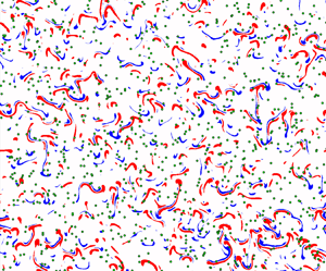
Widespread interaction between buoyancy-carrying blobs is clearly visible in figure 9. The blobs occupy a relatively small portion of the fluid (the solid and dashed contours in figure 9 enclose only 5 % of the total area). The rest of the fluid is constantly stirred by their motion. From this incoherent background, new blobs may occasionally emerge that take the place of those that have dissolved. Fluxes in the background are generally weak and positive: in a finger-favourable stratification, a vertical displacement of fluid nearly always results in a up-gradient flux, but if that portion of fluid does not have Goldilocks parameters, it will not maintain long-term coherence.

Figure 9. Instantaneous advective buoyancy flux in the central portion of the domain of the simulation with  $R_S=10^{14}$. The black lines are $\pm 0.0035$ buoyancy anomaly contours (negative dashed), corresponding to the average buoyancy anomaly of the longest legs in figure 1(b). The integral scale $l_\omega$ is the width of the green bar in the upper left corner.
The regions of the fluid that are more vigorously stirred by the blobs may actually develop down-gradient fluxes: figure 9 shows negative values either in the wake of a blob, or where two or more blobs interact vigorously. This supports the hypothesis set forth by Paparella & von Hardenberg (Reference Paparella and von Hardenberg2012) suggesting that vigorous enough fingering convection may produce so much down-gradient flux as to locally change the stratification.
We should stress that the Lagrangian particles on which this study is based do not necessarily track buoyancy, which is not a material invariant. Thus, Lagrangian particles could be ejected from a blob, or entrained in it, while it keeps its coherence. Furthermore, the cumulative flux fraction (3.2) is biased towards short legs, because in the time required for a particle to travel a long leg, another particle may perform several short legs, which are counted independently. Thus, if anything, our technique underestimates the level of vertical coherency of the buoyancy-carrying structures. However, we believe to have sufficiently underscored the usefulness of shifting to a Lagrangian description of fingering convection, hoping that this will lead to further progress on key issues, such as better flux parametrizations (e.g. for ocean models) and improved theories of staircase formation.
Finally, we should remark that, to be able to explore a regime where fingering convection is very vigorous without a prohibitive use of computational resources, in this paper, we consider the two-dimensional case. The in-depth review by Radko (Reference Radko2013, § 3.5), and the more recent results of Yang et al. (Reference Yang, Chen, Verzicco and Lohse2020), shows that two- and three-dimensional simulations are qualitatively equivalent, with well-documented small quantitative differences. The observation that fluxes are higher in three dimensions than in two may be suggestive of faster blobs, or of a reduced rate of interactions between blobs than in two dimensions. Thus, future work aimed at establishing quantitative parametrizations may benefit from three-dimensional simulations.
Supplementary material and movie
Supplementary material and movie is available at https://doi.org/10.1017/jfm.2023.311.
Acknowledgements
This work began during the Kavli Institute for Theoretical Physics program ‘Layering in Atmospheres, Oceans and Plasmas’ (Jan–Mar 2021). F.P. also acknowledges discussing the subject of this paper with Dr M. Bazot.
Funding
F.P. was supported by the New York University Abu Dhabi Research Institute grants CG002 (Center on Stability, Instability and Turbulence) and CG009 (Arabian Center for Climate and Environmental ScienceS). This work was supported in part through the NYUAD's Center for Research Computing resources, services and staff expertise.
Declaration of interests
The authors report no conflict of interest.
Data availability statement
All data and codes are available, upon request, from the authors.
Author contributions
H.L and F.P. contributed equally to this work.


 Open access