


INTRODUCTION
Varying climate conditions are recognized for the late-glacial (LG) interval across northeastern North America, but their regional expression remains relatively unknown. Proxy records from areas in and adjacent to the Great Lakes region suggest significant spatial and/or temporal differences in climate that result in a wide range of interpretations, many of which are still under debate (e.g., Edwards et al., Reference Edwards, Aravena, Fritz and Morgan1985; Fritz et al., Reference Fritz, Morgan, Eicher and McAndrews1987; Shane, Reference Shane1987; Tinkler and Pengelly, Reference Tinkler and Pengelly1994; Yu, Reference Yu2000; Yu and Wright, Reference Yu and Wright2001; Laub, Reference Laub2003b; Miller and Futyma, Reference Miller, Futyma and Laub2003; Webb et al., Reference Webb, Shuman, Leduc, Newby, Miller and Laub2003; Gonzales and Grimm, Reference Gonzales and Grimm2009; Renssen et al., Reference Renssen, Goosse, Roche and Seppä2018; Watson et al., Reference Watson, Williams, Russell, Jackson, Shane and Lowell2018; Fastovich et al., Reference Fastovich, Russell, Jackson and Williams2020; Renssen, Reference Renssen2020; Young et al., Reference Young, Gordon, Owen, Huot and Zerfas2020).
The established climate progression of the warming Bølling-Allerød – cold Younger Dryas – warm Early Holocene (BA-YD-EH) and its spatial extent came from evidence of climate change in the Greenland ice cores (e.g., Alley, Reference Alley2000, Reference Alley2004) and coeval changes in other proxy records from in and around the North Atlantic Ocean and beyond (e.g., Jacobson et al., Reference Jacobson, Webb, Grimm, Ruddiman and Wright1987; Peteet, Reference Peteet1995; Shuman et al., Reference Shuman, Webb, Bartlein and Williams2002; Dyke, Reference Dyke2005; Broecker, Reference Broecker2006; Williams and Shuman, Reference Williams and Shuman2008; Renssen et al., Reference Renssen, Goosse, Roche and Seppä2018; Renssen, Reference Renssen2020). However, the timing of changes in many of the proxies, especially for changes in the YD interval, is often based on the circular reasoning that changes similar to those in the Greenland ice cores were coeval rather than based on independent dates or on changes in better-dated proxy records in closer proximity to their respective sites (e.g., Miller and Gingerich, Reference Miller and Gingerich2013; Muschitiello and Wohlfarth, Reference Muschitiello and Wohlfarth2015; Watson et al., Reference Watson, Williams, Russell, Jackson, Shane and Lowell2018; Fastovich et al., Reference Fastovich, Russell, Jackson and Williams2020). Connection of records from the Great Lakes with the Greenland record requires independent dating due to distances, differences between continental and oceanic climates, and the possible effects of regional-scale factors.
Subfossil pollen assemblages of primarily spruce (Picea spp.), pine (Pinus spp.), and several non-arboreal species are established proxies of LG boreal climates in northeastern North America (e.g., Bartlein et al., Reference Bartlein, Prentice and Webb1986; Jacobson et al., Reference Jacobson, Webb, Grimm, Ruddiman and Wright1987; Webb et al., Reference Webb, Shuman, Leduc, Newby, Miller and Laub2003). Tamarack (Larix laricina) is not a key proxy due to its minimal pollen representation (e.g., Davis, Reference Davis1969; Birks, Reference Birks2003) but is often abundant in macrofossil collections (e.g., Shane, Reference Shane1987; Jackson et al., Reference Jackson, Overpeck, Webb, Keattch and Anderson1997). Tamarack is a pioneer species and tolerant to climate extremes more than spruce (Burns and Honkala, Reference Burns and Honkala1990), and these two features may add to current interpretations of climate change.
In this study, climate changes evident in the tree-ring widths of 55 subfossil logs from five sites in New York, USA, are shown to be significantly different from the BA-YD climate progression (Fig. 1) and coeval with hydrologic changes in the glacial Great Lakes (e.g., Lewis et al., Reference Lewis, King, Blasco, Brooks, Coakley, Crowley and Dettman2008, Reference Lewis, Cameron, Anderson, Heil and Gareau2012; Lewis and Anderson, Reference Lewis and Anderson2019). These findings suggest that the lakes were primary factors in regional climate dynamics and created a unique glacial lake-effect climate (GLEC) ~14.2 to 11.5 cal ka BP. Here we present a working hypothesis of this phenomenon.

Figure 1. (A) The overall increase in tree-ring widths during the late-glacial (LG) interval, first noted in the field and later confirmed by average ring widths (ARWs); (B) the Bølling-Allerød–cold Younger Dryas–warm Early Holocene (BA-YD-EH) temperature from the Greenland GISP2 ice core (Alley, Reference Alley2004). A regional climate anomaly is clearly apparent from the near inverse relationship between the tree-ring records and temperature reconstruction from the ice core data. In A, the juvenile rings are rings 1–35 and mature rings are rings 36–85 in each sample; the mean and median ARW values are used in t-tests and box-and-whisker diagrams, respectively. Phases P1early to P3 were identified by a clustering of the samples’ calibrated 14C dates over time and by differences in ARWs from phase to phase (Table 1).
Background
The present Great Lakes region comprises five lakes, all of which rank in the top 12 of the largest freshwater lakes in the world and have a combined surface area of ~245,000 km2. The lakes have mesoscale influence on climate above and around the lakes, particularly on their downwind sides (Scott and Huff, Reference Scott and Huff1996; Villani et al., Reference Villani, Jurewicz and Reinhold2017). The geography of the study region across New York State consists of the low-relief Erie–Ontario lowlands (EOL), including the Mohawk River valley, and the higher terrain of the northeastern Allegheny Plateau (AP) (Fig. 2), a region that has been on the downwind side of lakes since deglaciation. The topography of the EOL-AP is more variable east and north of the study region, with lower relief to the west across the lakes and interior lowlands.
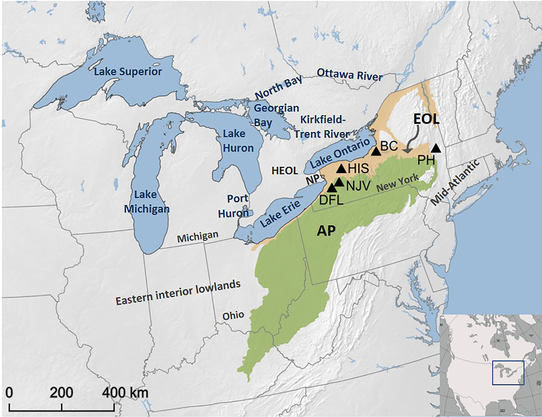
Figure 2. Map of the Great Lakes and study region, showing the lakes’ configuration and modern drainage system. The five study sites (DFL, Doerfel; NJV, North Java; HIS, Hiscock; BC, Bell Creek; and PH, Pump House) are on the Erie and Ontario lowlands (EOL) and Allegheny Plateau (AP) in New York State, USA. HEOL, lowlands between Lakes Huron, Erie, and Ontario; NP, Niagara Peninsula.
Between 14.2 and 10.5 cal ka BP, the glacial Great Lakes evolved from separate proglacial lakes in individual lake basins to an extensive glacial lake system, including the Great Lakes, Lake Agassiz, and the Lake Champlain basin, then back to separate lake basins with highly variable meltwater flow and no meltwater input anywhere near the EOL-AP (e.g., Lewis et al., Reference Lewis, Heil, Hubeny, King, Moore and Rea2007, Reference Lewis, King, Blasco, Brooks, Coakley, Crowley and Dettman2008, Reference Lewis, Cameron, Anderson, Heil and Gareau2012; Anderson and Lewis, Reference Anderson and Lewis2012; Lewis and Anderson, Reference Lewis and Anderson2017, Reference Lewis and Anderson2019; Fig. 3). The southern margin of the Laurentide Ice Sheet (LIS) was predominantly moving northward within the Great Lakes region during the study interval, with a pause in its movement north of the Lake Huron and Lake Ontario basins ca 12.8–12.1 ka and a southward movement of the Marquette Readvance in the Lake Superior basin ca 12.5–11.5 ka (Dyke et al., Reference Dyke, Moore and Robertson2003; Lowell et al., Reference Lowell, Fisher, Hajdasc, Glover, Loopee and Henry2009; Rayburn et al., Reference Rayburn, Cronin, Franzi, Knuepfer and Willard2011; Lewis and Anderson, Reference Lewis and Anderson2017, Reference Lewis and Anderson2019; Dalton et al., Reference Dalton, Margold, Stokes, Tarasov, Dyke, Adams and Allard2020; Fig. 3C and D). The LIS added to the topography within the lakes region, and its relatively stationary glacial anticyclonic circulation produced strong easterly surface winds south of the LIS, forcing the prevailing westerlies to the south (e.g., Rind, Reference Rind1987; Schaetzl et al., Reference Schaetzl, Krist, Lewis, Luehmann and Michalek2016; Conroy et al., Reference Conroy, Karamperidou, Grimley and Guenthner2019; Figs. 3 and 4). The westerlies likely evolved from the westerlies accompanying cold Pacific air masses to northwesterlies associated with polar dry air masses (e.g., Bryson, Reference Bryson1966; Rind, Reference Rind1987) and altered the incoming surface winds in the Great Lakes region (Fig. 4). In addition to all these changes, the changes in the lakes’ effects on weather patterns need to be considered as a viable factor in climate change but have been only occasionally considered (e.g., Saarnisto, Reference Saarnisto1974; Shane, Reference Shane1987; Shane and Anderson Reference Shane and Anderson1993). In the next section, we summarize current lake-effect features and consider the hydrologic processes of lakes in their interactions with meltwater, ice sheets, atmospheric circulation, and topography.
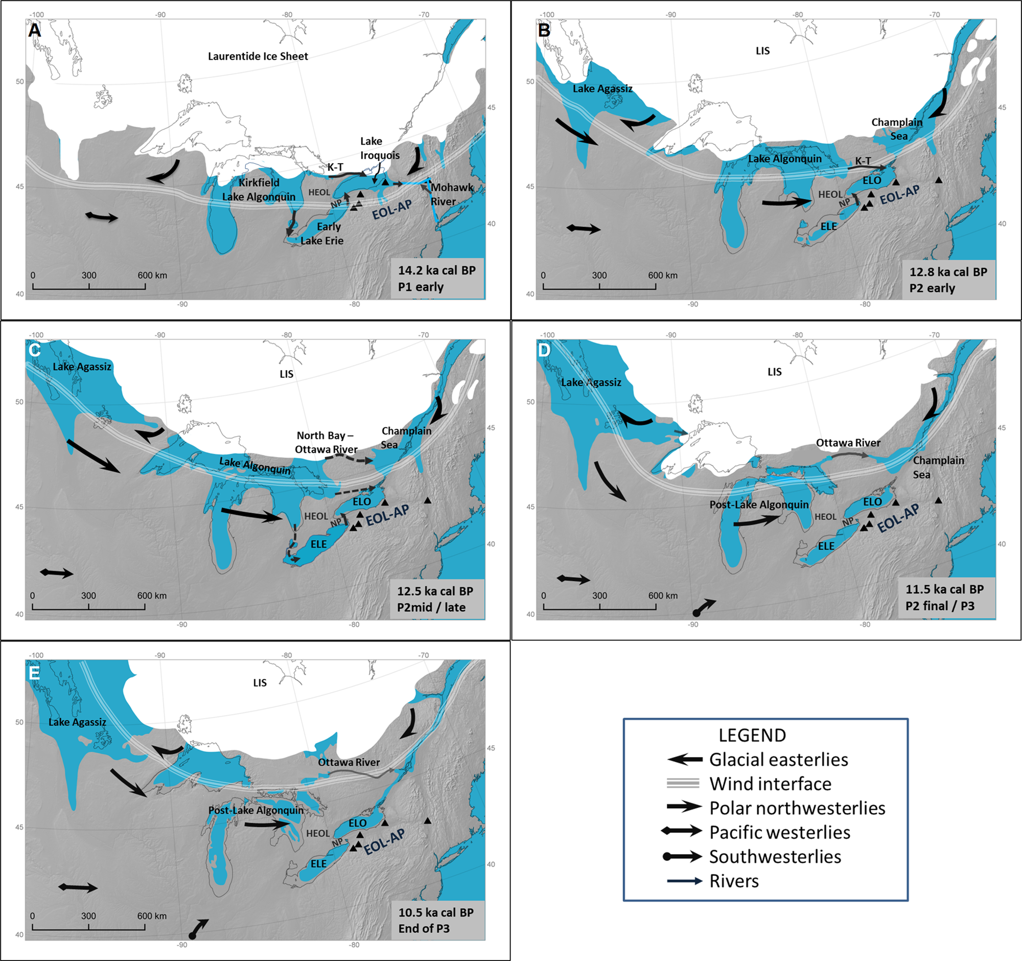
Figure 3. The paleogeography of the Great Lakes region in North America, 14.2–10.5 cal ka BP, illustrating changes in the lakes, position of the Laurentide Ice Sheet (LIS), meltwater distribution, and near-surface wind direction and speed over time. The approximate position of the easterly–westerly wind interface is at ~150 km from the LIS and ~50 km in width. (A) ~14.2 ka, the onset of phase P1: Lake Iroquois was expanding from meltwater directly off the LIS plus inflow from Early Lake Algonquin via Early Lake Erie (ELE), then via Kirkfield–Trent River (K-T) after ~13.8 ka. Winds across the Erie–Ontario lowlands–Allegheny Plateau (EOL-AP) were the glacial easterlies across Lake Iroquois and prevailing westerlies accompanying the Pacific air mass across ELE. (B) ~12.8 ka in P2early: Lake Iroquois and successor lakes were replaced by the initial Early Lake Ontario (ELO) and inflow continued from Lake Algonquin via K-T and ELE. Polar northwesterlies from around the western LIS were initiated. (C) ~12.5 ka at the P2early/P2mid transition, just before the North Bay–Ottawa River meltwater outlet opened from Lake Algonquin. Meltwater inflow into ELO was from Lake Algonquin via Kirkfield and perhaps ELE just before the opening of the new Lake Algonquin outlet. Northwesterlies were predominant across the EOL-AP. (D) 11.5 ka, P2 final/P3 transition. ELE and ELO attained their respective lowstands with the EOL-AP just within the southern reach of the unidirectional northwesterlies. (E) 10.5 ka, end of P3. The basins in the Great Lakes were all at their respective lowstands, and the wind interface was more than 300 km from the northern EOL-AP. (Maps accessed from Dyke et al. [Reference Dyke, Moore and Robertson2003], Dyke [Reference Dyke, Ehlers and Gibbard2004], and Dalton et al. [Reference Dalton, Margold, Stokes, Tarasov, Dyke, Adams and Allard2020], and revised by Keith Jenkins of the Cornell University Library GIS Services).

Figure 4. Proposed changes in wind sources and intensity across North America and their influence on the incoming winds across the Great Lakes during the late-glacial interval. The changes were derived from the position and movements of the Laurentide and Cordilleran Ice Sheets (LIS and CIS) and based on modern-day atmospheric circulation and glacial anticyclonic circulation (e.g., Rind, Reference Rind1987; Schaetzl et al., Reference Schaetzl, Krist, Lewis, Luehmann and Michalek2016, Renssen et al., Reference Renssen, Goosse, Roche and Seppä2018; Conroy et al., Reference Conroy, Karamperidou, Grimley and Guenthner2019). (A) 14.2 ka, P1 interval. Glacial easterlies traveled across the northern half of the Erie–Ontario lowlands–Allegheny Plateau (EOL-AP). Incoming westerlies came directly from the Pacific Ocean and were relatively weak. (B) 12.8 ka, P2early. Easterlies were above the Lake Ontario basin and stayed approximately in that position until ca. 11.7 ka, and the Champlain Sea added to its moisture level. Dry polar northwesterlies began to influence the Great Lakes surface winds. (C) 12.5 ka, P2early to P2mid transition. Dry polar northwesterlies traveled around the near-perfect arc of the LIS and wind interface and across southern Lake Agassiz and the Great Lakes. Easterlies continued to receive moisture from the Champlain Sea. (D) 11.5 ka, P2final/P3 transition. The LIS had started to move northward from the lakes, but the Marquette readvance moved the wind interface southward. The EOL-AP was just within the southern reach of the unidirectional northwesterlies. The southwesterlies began to be a key factor in the climate of the Great Lakes region. (E) 10.5 ka, P3. The northwesterlies continued to influence the Great Lakes, but the wind interface was more than 300 km from the northern EOL-AP, which ended the GLEC in the study region. The legend is the same as in Fig. 3. (Maps from Dyke et al. [Reference Dyke, Moore and Robertson2003], Dyke [Reference Dyke, Ehlers and Gibbard2004], and Dalton et al. [Reference Dalton, Margold, Stokes, Tarasov, Dyke, Adams and Allard2020], revised by Keith Jenkins of the Cornell University Library GIS Services).
Lake-effect climate dynamics
Lake-effect storms are the ultimate manifestation of a lake’s influence on climate (e.g., Passerelli and Braham, Reference Passerelli and Braham1981; Scott and Huff, Reference Scott and Huff1996; Laird et al., Reference Laird, Walsh and Kristovich2003; Long et al., Reference Long, Perrie, Gyakum, Caya and Laprise2007; Vavrus et al., Reference Vavrus, Notaro and Zarrin2012; Villani et al., Reference Villani, Jurewicz and Reinhold2017), but in addition to the storms, every large lake continuously affects mesoscale atmospheric circulation, surface air temperature and moisture content, and surface winds above and around the lake, especially on its downwind side (Sousounis and Fritsch, Reference Sousounis and Fritsch1994; Scott and Huff, Reference Scott and Huff1996). A lake’s spatial impact depends on factors such as lake size, fetch, ice-over versus open-water status, wind speed and direction, atmospheric stability, and regional topography, and extends farthest across low-relief topography on its downwind side (e.g., Libicki and Bedford, Reference Libicki and Bedford1990; Kristovich and Laird, Reference Kristovich and Laird1998; Samuelsson and Tjernström, Reference Samuelsson and Tjernström2001; Desai et al., Reference Desai, Austin, Bennington and McKinley2009; Vavrus et al., Reference Vavrus, Notaro and Zarrin2012; Veels and Steenburgh, Reference Veels and Steenburgh2015; Lang et al., Reference Lang, McDonald, Gaudet, Doeblin, Jones and Laird2018). Multiple lakes in close proximity increase the extent and strength of impact, and the greatest impact of lake effect from the Great Lakes today is up to 300 km downwind of Lakes Ontario and Erie across most of central New York, due to prevailing westerlies, the two lakes’ east-west orientation, and the presence of Lakes Huron, Michigan, and Superior on their upwind sides (Sousounis and Fritsch, Reference Sousounis and Fritsch1994; Scott and Huff, Reference Scott and Huff1996; Weiss and Sousounis, Reference Weiss and Sousounis1999; Mann et al., Reference Mann, Wagenmaker and Sousounis2002; Burnett et al., Reference Burnett, Kirby, Mullins and Patterson2003; Villani et al., Reference Villani, Jurewicz and Reinhold2017; Lang et al., Reference Lang, McDonald, Gaudet, Doeblin, Jones and Laird2018).
During the LG interval, the changing oceans, ice sheets, glacial anticyclonic winds, and meltwater distribution affected synoptic-scale climate dynamics (e.g., Rind, Reference Rind1987; Renssen et al., Reference Renssen, Goosse, Roche and Seppä2018; Conroy et al., Reference Conroy, Karamperidou, Grimley and Guenthner2019). The glacial Great Lakes certainly influenced mesoscale climate dynamics, but the physical characteristics and configuration of the lakes and ice sheet probably extended their influence on larger-scale dynamics to a regional scale (Long et al., Reference Long, Perrie, Gyakum, Caya and Laprise2007; Lowell et al., Reference Lowell, Fisher, Hajdasc, Glover, Loopee and Henry2009; Rayburn et al., Reference Rayburn, Cronin, Franzi, Knuepfer and Willard2011; Ullman et al., Reference Ullman, LeGrande, Carlson, Anslow and Licciardi2014; Lewis and Anderson, Reference Lewis and Anderson2017, Reference Lewis and Anderson2019; Dalton et al., Reference Dalton, Margold, Stokes, Tarasov, Dyke, Adams and Allard2020; Figs. 3 and 4). The easterlies produced by glacial anticyclonic circulation extended ~150 km south of the LIS (Schaetzl et al., Reference Schaetzl, Krist, Lewis, Luehmann and Michalek2016 and references therein), forcing the prevailing westerlies to the south. This wind pattern included easterly winds across one or more of the glacial lakes at any given time and highly variable surface winds at the interface between easterlies and westerlies at ~100–200 km south of the ice sheet (e.g., Ullman et al., Reference Ullman, LeGrande, Carlson, Anslow and Licciardi2014; Schaetzl et al., Reference Schaetzl, Krist, Lewis, Luehmann and Michalek2016; Renssen et al., Reference Renssen, Goosse, Roche and Seppä2018; Renssen, Reference Renssen2020; Figs. 3 and 4). Prevailing westerlies were likely increasingly strong up to ~200 km from the easterly–westerly wind interface as their proximity decreased, then progressively moderate farther south. The extent of influence from the easterlies was perhaps ~300 km from the interface and 400–500 km from the LIS (e.g., Schaetzl et al., Reference Schaetzl, Krist, Lewis, Luehmann and Michalek2016; Figs. 3 and 4).
On the synoptic scale, atmospheric circulation and the prevailing westerlies upwind of the lakes were likely altered by the relative position of the LIS and Cordilleran Ice Sheet (CIS) and their associated winds (e.g., Rind, Reference Rind1987; Atkinson et al., Reference Atkinson, Pawley and Utting2016; Utting et al., Reference Utting, Atkinson, Pawley and Livingstone2016; Figs. 3 and 4). From ~14.2 to 13.0 ka, the westerlies were the remains of the cool Pacific westerlies traveling across the Rocky Mountains; after 12.9 ka, the north-south corridor between ice sheets widened, and dry polar northwesterlies traveled around the glacial easterlies with limited orographic impact. The influence of warm southwesterly surface winds was likely minimal due to the strength of the prevailing westerlies south of the Great Lakes until after ca 11.5 ka in the Early Holocene interval (e.g., Edwards and Wolfe, Reference Edwards and Wolfe1996; Hostetler et al., Reference Hostetler, Bartlein, Clark, Small and Solomon2000; Figs. 3 and 4).
The glacial Great Lakes may have amplified the already-increased seasonality of the LG interval (e.g., Berger, Reference Berger1978; Solanki et al., Reference Solanki, Usoskin, Kromer, Schüssler and Beer2004; Hegerl et al., Reference Hegerl, Luterbacher, González-Rouco, Tett, Crowley and Xoplaki2011) due to their surface area, function as heat sink or heat source, and the significant differences in surface friction and albedo between frozen and open lake surfaces (Scott and Huff, Reference Scott and Huff1996; Blanken et al., Reference Blanken, Rouse and Schertzer2003; Rouse et al., Reference Rouse, Blyth, Crawford, Gyakum, Janowicz, Kochtubajda and Leighton2003; Cordeira and Laird, Reference Cordeira and Laird2008; Wright et al., Reference Wright, Posselt and Steiner2012).
Paleoenvironmental reconstruction
Tamarack is rarely used in climate interpretations due to its limited representation in pollen records (e.g., Davis, Reference Davis1969; Webb et al., Reference Webb, Laseski and Bernabo1978; Spear et al., Reference Spear, Davis and Shane1994; Pisaric et al., Reference Pisaric, MacDonald, Velichko and Cwynar2001; Birks, Reference Birks2003), which has made spruce species the primary indicators of boreal environments (e.g., Davis, Reference Davis1969; Anderson, Reference Anderson, Bryant and Holloway1985; Jacobson et al., Reference Jacobson, Webb, Grimm, Ruddiman and Wright1987; Dyke, Reference Dyke2005). Differences in the preferred habitats and tolerance of particular climatic and environmental conditions between tamarack and spruce suggest significant variations in moisture and temperature, particularly temperature extremes, on seasonal to multi-decadal timescales (e.g., Burns and Honkala, Reference Burns and Honkala1990; Vaganov et al., Reference Vaganov, Hughes, Kirdyanov, Schweingruber and Silkin1999; Jarvis and Linder, Reference Jarvis and Linder2000).
Tamarack is a pioneer species, intolerant of shade and sustained drought; grows best in well-drained soils; and is more tolerant of frequent climate extremes than spruce (Harlow et al., Reference Harlow, Harrar and White1979; Burns and Honkala, Reference Burns and Honkala1990 and references therein). White and black spruce (Picea glauca and P. mariana, respectively) are shade tolerant, but white spruce grows best on better-drained mineral soils, and black spruce grows in moister organic soils (Sutton, Reference Sutton1969; Burns and Honkala, Reference Burns and Honkala1990). Unfortunately, the identification of white versus black spruce is difficult when using wood or pollen, which is problematic for interpretation of atmospheric moisture content, but the two species are easily identifiable in smaller macrofossils, especially cones or twigs (Harlow, Reference Harlow1959; Schweingruber, Reference Schweingruber1990; Hoadley, Reference Hoadley1990). Tamarack tolerates extreme January temperatures of −55°C to −62°C, white and black spruce to −55°C, and the northern range limit of all three is where the average minimum January temperature (AMJT) is ~ −30°C (Burns and Honkala, Reference Burns and Honkala1990; Supplementary Table S1). Of cool-temperate species, black ash and northern white-cedar (F. nigra and Thuja occidentalis, respectively) tolerate the coldest AMJT, ca. −18°C, but only black ash tolerates the same temperature extremes as spruce and tamarack, ca. −50°C (Kreyling et al., Reference Kreyling, Schmid and Aas2015; Strimbeck et al., Reference Strimbeck, Schaberg, Fossdal, Schröder and Kjellsen2015). The establishment and survival of any thermophilous species in a boreal climate generally depends on factors such as the length of the growing season and extremes in temperature, particularly at the beginning or end of the growing season (Burns and Honkala, Reference Burns and Honkala1990; Sperry et al., Reference Sperry, Nichols, Sullivan and Eastlack1994; Vaganov et al., Reference Vaganov, Hughes, Kirdyanov, Schweingruber and Silkin1999; Jarvis and Linder, Reference Jarvis and Linder2000; Mielko and Woo, Reference Mielko and Woo2006), and conifers plus diffuse-porous species such as black ash survive better than other arboreal species when frequent freeze–thaw events occur (Sperry et al., Reference Sperry, Nichols, Sullivan and Eastlack1994).
The abundance of both pioneer tamarack and shade-tolerant spruce in the recovered logs and changes in their respective dominance over time plus the exclusivity of black ash offer a unique opportunity to identify changes in both environmental and climate conditions heretofore unknown.
MATERIALS AND METHODS
Materials
Subfossil logs were found at five LG sites in upstate New York (Fig. 2, Table 1). The Doerfel site (DFL) in Erie County (42.56°N, 78.71°W, 530 m above sea level [m asl]) and North Java (NJV) in Wyoming County (42.68°N, 78.33°W, 485 m asl) are spring-fed kettle ponds on the AP, and logs dating ca. 14.2–13.2 ka were recovered from the two sites (Laub and McAndrews, Reference Laub and McAndrews1999, Reference Laub and McAndrews2000; Griggs and Kromer, Reference Griggs, Kromer, Allmon and Nester2008; Laub, R.S., personal communication, 2006–2018; Fig. 2). The Hiscock site (HIS) in Genesee County (43.08°N, 78.08°W, 198 m asl) is composed of a spring-fed basin in the EOL with recovered wood fragments dating ca. 13.2 ka into the Early Holocene, but intact logs were rare due to the continual presence of wood-browsing mastodons (Laub et al., Reference Laub, Miller and Steadman1988; Laub, Reference Laub2003a b; Laub, R.S., personal communication, 2006–2018). Bell Creek (BC) in Oswego County (43.30°N, 76.34°W, 135 m asl) and Pump House (PH) in Albany County (42.78°N, 73.70°W, 48 m asl) are floodplain sites on the Ontario and Mohawk Valley lowlands, respectively, and their recovered logs date from ~12.8 ka into the Early Holocene (Miller and Griggs Reference Miller and Griggs2012; Griggs and Grote, Reference Griggs and Grote2016; Griggs et al., Reference Griggs, Peteet, Kromer, Grote and Southon2017; Fig. 2).
Table 1. List of phases and subphases, samples, diameter, average ring widths of juvenile, mature, and complete sequences, species, chronology name if applicable, and radiocarbon ages.a

a Abbreviations: Sites: NJV, North Java; DFL, Doerfel; HIS, Hiscock; BC, Bell Creek; PH, Pump House; Diam, diameter of the cross section; ARW, average ring width; Juv, Juvenile rings 1–35; Mat, mature rings 36–85; N, total ring count; Sp, species: PCSP, spruce species; LALA, tamarack; Rings dated, rings included in a 14C-dated segment, if known. Radiocarbon labs: Hd, Heidelberg; CAMS, Center for Accelerator Mass Spectrometry; WW, USGS Geoscience Center; UCIAMS, Keck Carbon Cycle AMS Laboratory; ISGS, Illinois State Geological Survey; Beta, Beta Analytic.
b DFL dates of findings found in situ above and below logs in analysis.
c PH logs are all tamarack, incorrectly listed as spruce in Miller and Griggs (Reference Miller and Griggs2012).
N.B. NJV, BC, and PH are revised site abbreviations for WWW (Griggs and Kromer, Reference Griggs, Kromer, Allmon and Nester2008), OBF (Griggs and Grote, Reference Griggs and Grote2016, Griggs at al., Reference Griggs, Peteet, Kromer, Grote and Southon2017), and HM/HMPHS (Miller and Griggs, Reference Miller and Griggs2012), respectively. Sample numbers are the same.
The logs recovered (used here) include 30 (15) at North Java, 6 (4) at Doerfel, 1 (1) at Hiscock, 58 (31) at Bell Creek, and 9 (4) at Pump House (Laub et al., Reference Laub, Miller and Steadman1988; Laub and McAndrews, Reference Laub and McAndrews1999, Reference Laub and McAndrews2000; Laub, Reference Laub2003b; Griggs and Kromer, Reference Griggs, Kromer, Allmon and Nester2008; Miller and Griggs, Reference Miller and Griggs2012; Griggs and Grote, Reference Griggs and Grote2016; Griggs et al., Reference Griggs, Peteet, Kromer, Grote and Southon2017). Substantive pollen and other macrofossils were previously analyzed for Pump House, Hiscock, and Doerfel (Laub et al., Reference Laub, Miller and Steadman1988; Miller, Reference Miller, Laub, Miller and Steadman1988; Laub and McAndrews, Reference Laub and McAndrews1999, Reference Laub and McAndrews2000; Futyma and Miller, Reference Futyma and NG Miller2001; Laub, Reference Laub2003b; Miller and Futyma, Reference Miller, Futyma and Laub2003; Miller and Griggs, Reference Miller and Griggs2012). An exploratory collection was analyzed for Bell Creek (Griggs and Grote, Reference Griggs and Grote2016; Griggs et al., Reference Griggs, Peteet, Kromer, Grote and Southon2017; Peteet, D.M., personal communication, 2015–2020), and North Java had no pollen analysis, but the site is within 20 km of Nichols Brook (Calkin and McAndrews, Reference Calkin and McAndrews1980; Karrow and Warner, Reference Karrow, Warner, Laub, Miller and Steadman1988; Laub et al., Reference Laub, Miller and Steadman1988).
Methods
The 55 logs used in this study met three necessary criteria: presence of pith, at least 35 rings, and a pith-to-bark radius of >4 cm to omit possible branch growth. Species were identified and ring widths measured; several tree-ring chronologies were compiled (e.g., Cook and Kairiukstis, Reference Cook and Kairiukstis1990; Hoadley, Reference Hoadley1990; Schweingruber, Reference Schweingruber1990; Griggs and Kromer, Reference Griggs, Kromer, Allmon and Nester2008; Miller and Griggs, Reference Miller and Griggs2012; Table 1), but only one chronology, 211 years in length, had the sample depth of 10 or more per year that is necessary for annual climate reconstruction (Griggs et al., Reference Griggs, Peteet, Kromer, Grote and Southon2017). This made annual climate reconstruction not viable for this study. Rather, based on our initial observations and using the biological ages of rings from pith to bark, the average ring widths (ARWs) of juvenile growth in rings 1–35 from the pith and mature growth in rings 36–85 were calculated and compared for possible evidence of environmental and climate changes on a multi-decadal timescale (e.g., Vaganov et al., Reference Vaganov, Hughes, Kirdyanov, Schweingruber and Silkin1999; Jarvis and Linder, Reference Jarvis and Linder2000). Box-and-whisker diagrams were used to identify changes, and two-tailed t-tests were used to identify significant changes in the ARWs over time.
For an assessment of climate conditions in the study interval, juvenile and mature ARWs were calculated from ring widths of 453 white spruce trees in 22 stands that cover most of the north-south range of white spruce across central and eastern Canada (International Tree-Ring Data Bank [ITRDB], available at https://www.ncdc.noaa.gov/data-access/paleoclimatology/tree-ring, accessed 2015–2019). Similar data were not available for tamarack or black spruce (Supplementary Fig. S1, Supplementary Table S1). The southern boundary of white spruce runs at approximately the 20°C average summer isotherm (Burns and Honkala, Reference Burns and Honkala1990), and the ARWs of white spruce were divided into 12 groups by the approximate distance of their respective sites to the southern boundary of the species range at the same longitude to acquire a data set representing relatively warmer summer temperatures on a N-S transect ending at the southern boundary. Those ARWs were used as representatives of spruce growing in northern, central, and southern boreal-type climates.
A timeline of possible climate changes in the LG interval was established from 14C dates of logs in situ at key stratigraphic positions and/or those with tree-ring growth patterns matching patterns in other dated samples and from 14C dates of additional materials associated with the logs. The 14C dates were calibrated and the 2σ calibrated error range was determined using the IntCal20 radiocarbon calibration curve (Reimer et al., Reference Reimer, Austin, Bard, Bayliss, Blackwell, Bronk Ramsey and Butzin2020) and OxCal v. 4.3 software (Bronk Ramsey et al., Reference Bronk Ramsey, van der Plicht and Weninger2001; http://c14.arch.ox.ac.uk/oxcal.html accessed 2020–2021) (Fig. 5). Several clusters of dates suggested by the calibrated years were used to group the samples into temporal phases, either where gaps between clusters were more than 100 years long or between a chronology and samples with no matching growth patterns.

Figure 5. The placement of the 47 radiocarbon dates from 33 samples, additional macrofossils, and associated bones (Table 1) on the IntCal20 calibration curve (Reimer et al., Reference Reimer, Austin, Bard, Bayliss, Blackwell, Bronk Ramsey and Butzin2020). Shaded columns are at the start of P1 and between phases and subphases. The wide column represents the hiatus of wood samples between P1 and P2; the date within the hiatus is of bone from the Hiscock site. The radiocarbon error bars are at the 2σ level and not visible where the range is smaller than the symbol. Bones and cone dates are represented by the smaller symbols of the corresponding site.
To test for climate change over time, the mean values of the ARWs in the main phases were tested for significant differences between phases using the box-and-whisker diagrams and two-tailed t-tests. The data sets of each phase were further divided by species and by sites to test for the possible influence of those factors on any significant differences between phases. The mean values and range of juvenile and mature ARWs of the main phases were also compared with the modern boreal forest data using the box-and-whisker diagrams to find whether they represented a northern, central, or southern boreal-type climate.
The main phases were then split into subphases in which smaller clusters were separated by less than 100 years, represented a tree-ring chronology, or contained only a few samples over a multi-century period. The mean values of the subphase ARWs were similarly tested for climate changes between subphases within and between the main phases.
Species representation of all logs plus other proxy records, including pollen, macrofossil, Coleoptera, firn, till, and eolian deposits found at sites within and immediately west, southwest, and northeast of the EOL-AP are included in this study (e.g., Morgan, Reference Morgan1972; Anderson, Reference Anderson, Bryant and Holloway1985; Filion, Reference Filion1987; Fritz et al., Reference Fritz, Morgan, Eicher and McAndrews1987; Shane, Reference Shane1987; David, Reference David and Gadd1988; Shane and Anderson, Reference Shane and Anderson1993; Tinkler and Pengelly, Reference Tinkler and Pengelly1994; Laub, Reference Laub2003b; Anderson and Lewis, Reference Anderson and Lewis2012; Schaetzl et al., Reference Schaetzl, Yansa and Luehmann2013; Watson et al., Reference Watson, Williams, Russell, Jackson, Shane and Lowell2018; Fastovich et al., Reference Fastovich, Russell, Jackson and Williams2020; Young et al., Reference Young, Gordon, Owen, Huot and Zerfas2020). They are used in interpreting climate change and the extent of the lake-effect climate using features such as the modern range of their respective species, their capability of withstanding climate extremes, and/or their physical characteristics.
RESULTS
Of the 55 samples meeting the necessary criteria, 27 are tamarack and 28 spruce (Table 1). For all samples, the ARWs range from 0.62 to 2.18 mm for the juvenile data and from 0.35 to 1.49 mm for the mature data (Table 1) with a slightly higher range of tamarack ARWs (for the juvenile segments: tamarack, 0.62–2.18 mm; spruce, 0.66–1.80 mm; for the mature rings: tamarack, 0.36–1.49 mm; spruce, 0.35–1.14 mm; Table 1). The modern ARWs of white spruce range from 0.05 to 4.10 mm (juvenile) and 0.05 to 3.50 mm (mature), suggesting that these trees grew in climate conditions typical of the boreal region today.
Forty-seven 14C dates were taken from one or more segments of rings in 33 of the 55 samples, and the other 22 samples were placed in time by their association with other dated samples and other materials (Fig. 5, Table 1). From their distribution and clustering on the calibration curve, three main phases, P1 at 14.2–13.1 ka, P2 at 12.9–11.5 ka, and P3 at 11.5–10.5 ka, were chosen (Fig. 5, Tables 1 and 2), all of which are over the 200+ year length considered necessary to represent regional rather than local climate change (e.g., Bartlein et al., Reference Bartlein, Prentice and Webb1986).
Table 2. Summary of the data sets within phases and subphases: range of dates, average and sample counts of the juvenile and mature average ring widths (ARWs), and represented species for each time interval.

a The species counts suggest co-dominance, except in P2mid, where only tamarack was represented, and P2final, when spruce was likely dominant.
A significant increase in both juvenile and mature ARWs from P1 to P2 is indicated by the box-and-whisker diagrams and t-tests between phases and between species and sites within phases (Fig. 6A–C, Table 3A–F). A northern boreal-type forest is suggested by the ARWs of P1 and a southern boreal-type forest by the ARWs of P2 (Fig. 6). The ARWs show a slight increase from P2 to P3 (Fig. 6A–C), suggesting climate conditions farther south than in P2 (Fig. 7), but the t-test is insignificant, and the small sample count and representation of only one site in P3 leaves any interpretation of change between P2 and P3 tentative only.

Figure 6. Box-and-whisker diagrams of the juvenile and mature average ring width (ARW) data sets. (A) ARWs in the three main phases. (B) ARWs further divided by species; (C) ARWs divided by phases and sites: North Java (NJV) and Doerfel (DFL) are in P1; Hiscock (HIS), Bell Creek (BC), and Pump House (PH) are in P2; and the Early Holocene (EH) samples from BC are in P3. (D) ARWs of samples in the six subphases and EH. The supporting t-statistics and P values are listed in Table 3. The boxes contain the 2nd and 3rd quartile data points; the horizontal lines are the median values; whiskers include at least 90% of the data points; diamonds represent outliers. Single horizontal lines (no box) represent the ARW of one sample. The bar charts along the x-axis of each diagram represent the sample counts per data set with its scale on the right y-axis.

Figure 7. The spruce ARWs from this study compared with those of samples from more than 500 white spruce trees in boreal forests across central and eastern Canada, North America (International Tree-Ring Data Bank [ITRDB], https://www.ncdc.noaa.gov/data-access/paleoclimatology/tree-ring, accessed 2015–2019) in box-and-whisker plots (see Fig. 6 caption). The y-axis is the approximate distance from the southern boundary of the range of white spruce to the location of each modern site at the same longitude. Only spruce samples were tested here due to the limited tamarack data on the ITRDB (Supplementary Fig. S1, Supplementary Table S1).
Table 3. The results of the t-tests used to identify significant differences in the mean values of the juvenile and mature average ring widths (ARWs) between the phases, species, sites, and subphase data sets over time (Fig. 6).a

a Positive t-values indicate an increase in ARWs from the left to right of compared data sets and vice versa. Bold values indicate significantly different data sets with P < 0.01 or 0.05; standard font indicates significant values at P < 0.10; “NS” indicates that the data sets are not significantly different. The tests contain ≥ 4 samples in both data sets except for the italicized t-values where one of the data sets has only 3 samples and the “Too few” tests where one or both data sets have < 3 samples.
Phases P1 and P2 were divided into six subphases by smaller clusters and chronologies: P1early and P1late and P2early, P2mid, P2late, and P2final (Figs. 5 and 6D, Table 2). All subphases are also at or over the 200 year minimum length requirement for representing regional change.
There is no significant change in ARWs between subphases P1early and P1late, although a slight decrease in the ARWs is suggested in the box-and-whisker diagrams (Fig. 6D, Table 3D1). As expected from the positive trend between main phases P1 and P2, the progression from a northern to southern boreal forest is evident between subphases P1late and P2early (Fig. 6D, Table 3D2). Within P2, the only significant differences in ARWs are a possible increase from P2early to P2mid and a significant decrease from P2mid to P2late and P2final (Fig. 6D, Tables 2 and 3D1). Only tamarack is represented in P2mid (Table 2), but t-tests between the ARWs of P2mid and in the other P2 subphases showed that the increase and decrease are not species specific (Fig. 6D, Table 3E). The increase and significant t -tests between ARWs of subphase P2final and P3 (Fig. 6D, Table 3D2) supports the transition from a southern to more southern boreal climate suggested between the ARWs of P2 and P3.
For species representation, more than 90% of all recovered logs and macrofossils from the five study sites are tamarack or spruce, and the two species are equally represented, except at Pump House, where tamarack, spruce, and balsam fir (Abies balsamea) are equally represented (Miller and Griggs, Reference Miller and Griggs2012; Table 1). During all phases and subphases, tamarack and spruce are suggested to be codominant, except for the exclusivity of tamarack logs in P2mid and the dominance of spruce in P2final (Table 2). Other tamarack macrofossils were present at all sites, and pollen representation was predictably low (Laub and McAndrews, Reference Laub and McAndrews1999, Reference Laub and McAndrews2000; Miller and Griggs, Reference Miller and Griggs2012; Peteet, D.M., personal communication, 2015–2020). Recovered spruce cones and other identified macrofossils represent only white spruce at Bell Creek and Pump House (P. glauca; Laub and McAndrews, Reference Laub and McAndrews1999, Reference Laub and McAndrews2000; Miller and Griggs, Reference Miller and Griggs2012; Griggs and Grote, Reference Griggs and Grote2016). Significant variations in spruce pollen percentages during ~P2mid into P3 were evident at Bell Creek (Peteet, D.M., personal communication, 2015–2020).
In the other ~10% of logs dating from 14.2 to at least 11.9 ka, species include the boreal species of balsam fir, poplar, and paper birch (A. balsamea, Populus spp., Betula papyrifera, respectively) plus black ash which dates back to at least ~13.25 ka (Laub and McAndrews, Reference Laub and McAndrews1999). In the upper LG and lower EH deposits, ~11.9 to 10.5 ka, around 50% of the logs are spruce or tamarack, with an increase in balsam fir and black ash and the first representation of the thermophilous northern white-cedar, red and eastern white pine, American elm, and red maple (T. occidentalis, Pinus resinosa, P. strobus, Ulmus americana, and Acer rubrum, respectively; Laub et al., Reference Laub, Miller and Steadman1988; Griggs and Kromer, Reference Griggs, Kromer, Allmon and Nester2008; Miller and Griggs, Reference Miller and Griggs2012; Griggs and Grote, Reference Griggs and Grote2016; Griggs, C.B., unpublished data).
Four takeaway points from the results are evident. First is the three main phases and six subphases identified from high-resolution 14C dating and significant differences in ARWs and species representation over time. Second is the major change in ARWs between P1 and P2 that suggests a transition from northern to southern-type boreal climate, both with possible non-analog features. Third is the minor changes in ARWs and species presence between several subphases. Fourth is the abundance of tamarack and sole representation of black ash for thermophilous species, in addition to spruce. All points support the interpretation of lake-effect climate in the following sections.
EVOLUTION OF ENVIRONMENT AND CLIMATE
In this section, the GLEC and its progression over time are interpreted from changes in the ARWs, species representation, and other proxy records from both the EOL-AP and the lowlands between the Lake Huron, Erie, and Ontario basins (HEOL; Fig. 2). The interpretations are extrapolated to the southwestern AP and interior lowlands (Fig. 2) to examine possible changes in the extent of the lakes’ effects on climate over time.
Phase 1 (P1), ~14.2–13.1 ka
P1early, ~14.2–13.8 ka
The ARWs in P1early suggest the northern boreal climate of today (Fig. 7, Table 2), but the exclusivity of black ash for cool-temperate species suggests a more central boreal zone that is the northern boundary of that species’ range today. A northern boreal climate is also seen in the high dominance of spruce with minimal thermophilous species in many pollen records from the EOL-AP and HEOL (e.g., Miller, Reference Miller1973; Yu, Reference Yu2000; Futyma and Miller, Reference Futyma and NG Miller2001; Miller and Futyma, Reference Miller, Futyma and Laub2003; Dyke, Reference Dyke2005), but both northern and southern boreal-type summer ecozones are suggested by Coleoptera species, agreeing with the warmer summer conditions suggested by the black ash (Edwards et al., Reference Edwards, Aravena, Fritz and Morgan1985; Fritz et al., Reference Fritz, Morgan, Eicher and McAndrews1987). These proxies suggest a non-analog northern boreal environment and high seasonality between summers and winters, possibly greater than caused by the solar and orbital forcings alone.
P1late, ~13.7–13.1 ka
Moister and perhaps slightly cooler growing conditions in a north-central boreal climate are suggested by the minimum ARWs of P1late but are not significantly different from P1early (Fig. 6D, Table 3D1). However, moister and cooler conditions are supported by substantial ice accumulation in the western EOL-AP and permafrost, oxygen isotopes, and firn on the Niagara Peninsula (Miller, Reference Miller1973; Mott and Farley-Gill, Reference Mott and Farley-Gill1978; Edwards et al., Reference Edwards, Aravena, Fritz and Morgan1985; Tinkler and Pengelly, Reference Tinkler and Pengelly1994; Young et al., Reference Young, Gordon, Owen, Huot and Zerfas2020).
The hiatus, ~13.1–12.9 ka
The increase in ARWs between P1 and P2 suggests a transition from northern boreal- to southern boreal-type climate (Fig. 7), but the lack of logs gives no higher temporal resolution to this change, thus the term “hiatus.” A transition to warmer and drier summer conditions is suggested in Coleoptera and a few pollen records (Miller and Morgan, Reference Miller and Morgan1981; Edwards et al., Reference Edwards, Aravena, Fritz and Morgan1985; Fritz et al., Reference Fritz, Morgan, Eicher and McAndrews1987; Motz and Morgan, Reference Motz and Morgan2001; Webb et al., Reference Webb, Shuman, Leduc, Newby, Miller and Laub2003). Warmer and drier conditions are also plausible in the reduction of ice and firn in the EOL-AP and HEOL (e.g., Miller, Reference Miller1973; Edwards et al., Reference Edwards, Aravena, Fritz and Morgan1985; Fritz et al., Reference Fritz, Morgan, Eicher and McAndrews1987; Tinkler and Pengelly, Reference Tinkler and Pengelly1994; Young et al., Reference Young, Gordon, Owen, Huot and Zerfas2020).
Phase 2 (P2), ~12.9–11.5 ka
In P2, the ARWs plus Coleoptera species suggest a southern boreal-type ecozone for summer in the EOL-AP and HEOL (Edwards et al., Reference Edwards, Aravena, Fritz and Morgan1985; Fritz et al., Reference Fritz, Morgan, Eicher and McAndrews1987; Miller and Morgan, Reference Miller and Morgan1981, Motz and Morgan, Reference Motz and Morgan2001; Fig. 7). However, the continuing exclusivity of black ash in most if not all of P2 suggests conditions such as colder and more variable winter temperatures and/or frequent freeze–thaw events during the growing season prohibited the establishment of additional thermophilous species.
The transition to a southern boreal summer climate between P1 and P2 sometime between 13.1 and 12.9 ka directly contrasts with the 12.9 ka transition from the warming BA to colder YD climate outside the lakes region (Fig. 1). The increase in annual variability in climate conditions and/or in seasonality from warming summers to continuing cold winters suggests that the annual cycle of open and frozen lakes plus length of transitions between the two were primary factors in GLEC dynamics.
P2early, ~12.9–12.5 ka
The ARWs indicate a southern boreal-type climate in summer, but species representation continues to suggest harsh winters in P2early. In Webb et al. (Reference Webb, Shuman, Leduc, Newby, Miller and Laub2003), a significant warming of both summer and winter temperatures in the western EOL-AP is based on changes in pollen percentages, but the non-inclusion of tamarack due solely to its low representation in pollen records likely exaggerated the proposed increase in summer temperatures and certainly raises questions about an increase in winter temperatures.
P2mid, ~12.5–11.9 ka
An increase in flooding or other environmental disturbance and/or more frequent climate extremes is suggested by the higher ARWs and exclusivity of tamarack (Fig. 6D, Tables 2 and 3E), both indicators of an open landscape and frequent site disruption for the ~600 year duration of P2mid. The higher ARWs suggest warmer temperatures, but the open terrain may be the main factor for good growth. The disturbances and extremes are also suggested by a slight decrease in spruce pollen, an increase in tamarack needles, and/or higher percentages of non-arboreal pollen across the EOL-AP and HEOL (e.g., Miller, Reference Miller1973; Fritz et al., Reference Fritz, Morgan, Eicher and McAndrews1987; Karrow and Warner Reference Karrow, Warner, Laub, Miller and Steadman1988; Tinkler et al., Reference Tinkler, Pengelly, Parkins and Terasmae1992; Yu, Reference Yu2000). Similarly, an open environment with flowing water in a southern boreal/cool-temperate summer climate is suggested by Coleoptera species (Fritz et al., Reference Fritz, Morgan, Eicher and McAndrews1987; Calkin and McAndrews, Reference Calkin and McAndrews1980, Miller and Morgan, Reference Miller and Morgan1981; Motz and Morgan, Reference Motz and Morgan2001). Harsh winters continued to restrict establishment of additional cool-temperate species.
P2late, ~11.9–11.7 ka
A return to a less variable, drier climate and the succession of pioneer to climax tree species in P2late is indicated by the ARWs, equivalent to the ARWs of P2early, and codominance of spruce and tamarack (Figs. 1 and 6, Table 2). Drier conditions are also indicated by the represented Coleoptera species (e.g., Fritz et al., Reference Fritz, Morgan, Eicher and McAndrews1987). Harsh winters continued.
P2final, ~11.7–11.5 ka
The dominance of spruce and reduced ARWs indicate a more closed forest in a climax environment, with tamarack growing mainly along streambanks or shorelines, suggesting the continuation of the drier and less variable southern boreal-type conditions. A less variable climate is also indicated by substantial forest floor litter and the continuation of the same Coleoptera species. No abrupt climate change is indicated by the ARWs or annual ring growth during the LG-EH transition, ca 11.7–11.5 ka (Griggs et al., Reference Griggs, Peteet, Kromer, Grote and Southon2017). However, an alleviation of the harsh winters may have begun by the end of this phase, suggested by the increase of thermophilous species from the upper LG/lower EH deposits.
Phase 3 (P3), ~11.5–10.5 ka
The tentative increase in ARWs only suggests a transition from a south-central boreal to a mixed boreal/cool-temperate ecosystem by the start of this phase (Figs. 1, 6A, and 7, Tables 2 and 3D2), but the transition and decreased seasonality is clearly indicated by the decrease in tamarack and spruce and the additional thermophilous species in the logs. These conditions suggest the end of the GLEC in the EOL-AP region.
PROPOSED ROLE OF LAKE-EFFECT PROCESSES ON CLIMATE
Here we give an interpretation of the glacial lakes’ effects on climate, including the inception, changing dynamics, and demise of the GLEC based on the evolution of climate discussed earlier and our current understanding of the glacial lake system and change plus ice sheets, meltwater, topography, and associated winds. Finally, we discuss the significance of the presence of both tamarack and black ash and its implications for the interpretation of the GLEC in the Great Lakes region and in climate reconstruction in general.
Onset of the GLEC
The GLEC across the EOL-AP likely began when easterlies traveled across the deglaciated Lake Erie basin onto the interior lowlands west of the EOL-AP before deglaciation of the Lake Ontario basin, but the single lake and wind direction was likely insufficient to produce a regional-scale regime (Laird et al., Reference Laird, DesRochers and Payer2009). More likely, the lake-effect climate was initiated from the northward expansion of Lake Iroquois (Fig. 3A) and northward movement of the easterly–westerly wind interface resulting in easterlies across Lake Iroquois and westerlies across Early Lake Erie (ELE; Fig. 3A). Changes in the lake-effect climate system in the following years, ca 14.2–10.5ka, are based on probable linkage of changes in climate to those in the hydrologic and glacial conditions. The following interpretations are rough estimates of those linkages.
Phase 1, ~14.2–13.1 ka
P1early, ~14.2–13.8 ka
The northern boreal climate suggested by the ARWs and species representation coincided with an expanding Lake Iroquois, ELE, and meltwater drainage through the EOL-AP via the Mohawk and Hudson Rivers (Eschman and Karrow, Reference Eschman, Karrow, Karrow and Calkin1985; Kaiser, Reference Kaiser1994; Lewis et al., Reference Lewis, Cameron, Anderson, Heil and Gareau2012; Lewis and Anderson, Reference Lewis and Anderson2019; Fig. 3A). The wind interface was located across the EOL-AP, with Lake Iroquois to the north of the interface and ELE to the south (Dyke et al., Reference Dyke, Moore and Robertson2003; Dalton et al., Reference Dalton, Margold, Stokes, Tarasov, Dyke, Adams and Allard2020; Fig. 3A). Easterlies traveled across the ~300 km fetch of Lake Iroquois and westerlies across the ~350 km fetch of ELE and likely produced copious amounts of precipitation along the interface, especially in the fall, when lakes were heat sources and evaporation rates were high and air temperatures were lower than water temperatures. The effects of open versus frozen lakes on the surface winds induced a greater seasonality.
P1late, ~13.7–13.1 ka
The cooler and/or wetter climate conditions suggested by the proxy records is coincidental with the expansion of Lake Iroquois to the north and east and continuing drainage into the Mohawk River Valley in the EOL-AP. The direct meltwater input from the LIS into Lake Iroquois was replaced by input via the much shorter Kirkfield-Trent Valley route to the north of the lake, which brought cooler meltwater into the lake than did meltwater input via ELE (Eschman and Karrow, Reference Eschman, Karrow, Karrow and Calkin1985; Kaiser, Reference Kaiser1994; Lewis et al., Reference Lewis, Cameron, Anderson, Heil and Gareau2012; Lewis and Anderson, Reference Lewis and Anderson2019; Fig. 3A). Meltwater inflow into ELE had ceased ca. 13.8 ka BP, which increased that lake's temperature and evaporation rate, but the end of meltwater inflow also reduced the size and output of the ELE, which in turn reduced its influence on the westerly winds, surface air temperatures, and perhaps the spatial extent of the GLEC (Eschman and Karrow, Reference Eschman, Karrow, Karrow and Calkin1985; Coakley and Lewis, Reference Coakley, Lewis, Karrow and Calkin1985; Tinkler et al., Reference Tinkler, Pengelly, Parkins and Terasmae1992; Lewis et al., Reference Lewis, Cameron, Anderson, Heil and Gareau2012).
To the east, the Champlain Sea was expanding, which increased the level of moisture in the easterlies (e.g., Pair and Rodrigues, Reference Pair and Rodrigues1993; Rayburn et al., Reference Rayburn, Cronin, Franzi, Knuepfer and Willard2011). At the wind interface, the extra moisture in both winds plus the higher temperature in the westerlies and lower temperature in the easterlies produced copious amounts of precipitation in the HEOL and EOL-AP. An ice advance in the western EOL-AP at 13.3–13.0 ka, the end of P1late into the hiatus, is proposed by Young et al. (Reference Young, Gordon, Owen, Huot and Zerfas2020). Those dates were estimated from findings at sites along the Genesee River and Cattaraugus Creek floodplains in the western AP, but the 2σ ranges of calibrated dates of wood and bone are ca. 13.8–13.2 ka at Doerfel located < 20 km Cattaraugus Creek, ca. 13.5–13.1 ka at North Java II between the two floodplains, and ca. 13.2–12.6 ka for the oldest dates at Hiscock at ~50 km west of the Genesee River floodplain. The ranges of these dates indicate an overall ice-free landscape on at least the higher elevations and relatively flat terrains from 13.3 to 13.0 ka. A possible alternative to an ice advance may have been increased precipitation and significant but isolated ice accumulations on the floodplains and more variable terrain. The suggested minimum ARWs plus ice accumulation and permafrost in both the EOL-AP and on the Niagara Peninsula (NP; Miller, Reference Miller1973; Edwards et al., Reference Edwards, Aravena, Fritz and Morgan1985; Tinkler and Pengelly, Reference Tinkler and Pengelly1994; Young et al., Reference Young, Gordon, Owen, Huot and Zerfas2020) in P1late suggest that the expansion of Lake Iroquois and reduction of ELE may have pushed the wind interface farther south onto the EOL-AP. The minimum ARWs and possible maximum ice accumulation on the EOL-AP (Young et al., Reference Young, Gordon, Owen, Huot and Zerfas2020) date to around the end of P1late and are also coeval with a brief but intense outburst of meltwater from Lake Agassiz that flowed briefly into ELE sometime between 13.2 and 12.9 ka and may have contributed to a cold and moist climate during the end of P1late and into the hiatus (Morgan, Reference Morgan1972; Eschman and Karrow, Reference Eschman, Karrow, Karrow and Calkin1985; Farrand and Drexler, Reference Farrand, Drexler, Karrow and Calkin1985; Teller, Reference Teller, Ruddiman and Wright1987; Tinkler et al., Reference Tinkler, Pengelly, Parkins and Terasmae1992; Rayburn et al., Reference Rayburn, Cronin, Franzi, Knuepfer and Willard2011; Leydet et al., Reference Leydet, Carlson, Teller, Breckenridge, Barth, Ullman, Sinclair, Milne, Cuzzone and Caffee2018).
The hiatus, ~13.1–12.9 ka
A change in GLEC from a northern to southern boreal-type and drier climate, suggested by the increase in ARWs from P1 to P2 and in changes in other proxy records, is coeval with the transition of Lake Iroquois to progressively smaller lakes from the rerouting of its output to the NE corner of the Lake Ontario basin, ending meltwater drainage via the Mohawk River into the EOL-AP (Pair and Rodrigues, Reference Pair and Rodrigues1993; Dyke et al., Reference Dyke, Moore and Robertson2003, Rayburn et al., Reference Rayburn, Knuepfer and Franzi2005, Reference Rayburn, Cronin, Franzi, Knuepfer and Willard2011; Anderson and Lewis, Reference Anderson and Lewis2012; Lewis and Todd, Reference Lewis and Todd2019; Lewis and Anderson, Reference Lewis and Anderson2019; Dalton et al., Reference Dalton, Margold, Stokes, Tarasov, Dyke, Adams and Allard2020; Fig. 3A and B). These changes alone likely increased summer temperatures and length of the growing season, but the wind interface was also moving north (Fig. 3A and B). By the end of the hiatus, both the Lake Ontario basin and ELE were south of the wind interface, which ended the copious amounts of precipitation across the EOL-AP and HEOL. However, the overall reduction in fetch of the lakes, position of the wind interface, and ongoing transition of incoming westerlies from Pacific westerlies to drier polar northwesterlies suggest that harsh winters continued (Fig. 4A and B).
Phase 2, ~12.9–11.5 ka
During P2, the GLEC was likely a southern boreal-type climate in summer but with a northern boreal-type winter. Changes between the subphases again can be linked to hydrologic changes, plus the position of the ice sheet and significant changes in the surface winds.
P2early, ~12.9–12.5 ka
The ARWs indicate that a southern boreal-type climate was established across the EOL-AP by the start of P2early, ~12.9 ka, concurrent with increasing lake surface area, the wind interface north of the Lake Ontario basin, and an overall reduction in meltwater flow south of the interface, including the absence of meltwater in ELE (Eschman and Karrow, Reference Eschman, Karrow, Karrow and Calkin1985; Farrand and Drexler, Reference Farrand, Drexler, Karrow and Calkin1985; Pair and Rodrigues, Reference Pair and Rodrigues1993; Webb et al., Reference Webb, Shuman, Leduc, Newby, Miller and Laub2003; Rayburn et al., Reference Rayburn, Knuepfer and Franzi2005, Reference Rayburn, Cronin, Franzi, Knuepfer and Willard2011; Anderson and Lewis Reference Anderson and Lewis2012; Lewis et al., Reference Lewis, Cameron, Anderson, Heil and Gareau2012; Watson et al., Reference Watson, Williams, Russell, Jackson, Shane and Lowell2018; Leydet et al., Reference Leydet, Carlson, Teller, Breckenridge, Barth, Ullman, Sinclair, Milne, Cuzzone and Caffee2018; Lewis and Todd, Reference Lewis and Todd2019; Fig. 3B). These conditions suggest increasing atmospheric temperatures and moisture content across the EOL-AP during P2early. However, the incoming westerlies had transitioned from cool Pacific westerlies to cold dry northwesterlies as the north-south corridor between the LIS and CIS widened (Dyke et al., Reference Dyke, Moore and Robertson2003; Atkinson et al., Reference Atkinson, Pawley and Utting2016; Utting et al., Reference Utting, Atkinson, Pawley and Livingstone2016; Figs. 3B and C and 4B and C).
Outside the EOL-AP and HEOL, warmer conditions and different timelines of climate change are also suggested by spruce/pine pollen transitions in the southwestern AP and by pollen and the biomarkers of archaeal brGDGT (branched glycerol dialkyl glycerol tetraether membrane lipids) found in the lowlands west of the plateau (Shane, Reference Shane1987; Shane and Anderson, Reference Shane and Anderson1993; Watson et al., Reference Watson, Williams, Russell, Jackson, Shane and Lowell2018). However, the 12.9 ka onset of the YD cold interval is suggested at other interior lowland sites by pollen and brGDGT analyses (e.g., Gonzales and Grimm, Reference Gonzales and Grimm2009; Fastovich et al., Reference Fastovich, Russell, Jackson and Williams2020). These spatial differences suggest a changing boundary of the GLEC due to changes in the downwind side of the lakes and spatial extent of the GLEC over time.
By the end of P2early, ca 12.5 ka, the lake surface area south of the wind interface was at its maximum (Eschman and Karrow, Reference Eschman, Karrow, Karrow and Calkin1985; Farrand and Drexler, Reference Farrand, Drexler, Karrow and Calkin1985; Lowell et al., Reference Lowell, Larson, Hughes and Denton1999, Reference Lowell, Fisher, Hajdasc, Glover, Loopee and Henry2009; Dyke et al., Reference Dyke, Moore and Robertson2003; Lewis et al., Reference Lewis, Cameron, Anderson, Heil and Gareau2012; Lewis and Todd, Reference Lewis and Todd2019; Fig. 3C), and the interaction between lakes and northwesterlies may have been at its peak due to the maximum size of the lakes, configuration of the lakes and LIS, and the near-perfect arc of the southern LIS.
The southern boreal climate suggested by the ARWs coincides with the multiple open lakes preventing the cold northwesterlies from lowering summer temperatures in the EOL-AP and HEOL (Figs. 3B and C and 4B and C). However, frozen lakes had limited interaction with the winds, and the southern margin of the LIS may have increased the harshness of winter climate conditions.
P2mid, ~12.5–11.9 ka
A greater variation in climate with a more open environment is suggested by the sole representation of tamarack and higher ARWs, and it began with the opening of the North Bay–Ottawa River outlets of Lake Algonquin ca. 12.5 ka, which terminated any meltwater inflow into both ELE and Early Lake Ontario (ELO) and altered configuration and increased water temperatures of the lakes (Eschman and Karrow, Reference Eschman, Karrow, Karrow and Calkin1985; Teller, Reference Teller, Ruddiman and Wright1987; Lowell et al., Reference Lowell, Larson, Hughes and Denton1999; Dyke et al., Reference Dyke, Moore and Robertson2003; Lewis et al., Reference Lewis, Heil, Hubeny, King, Moore and Rea2007, Reference Lewis, King, Blasco, Brooks, Coakley, Crowley and Dettman2008; Anderson and Lewis, Reference Anderson and Lewis2012; Hladyniuk and Longstaffe, Reference Hladyniuk and Longstaffe2016; Lewis and Anderson, Reference Lewis and Anderson2017, Reference Lewis and Anderson2019; Leydet et al., Reference Leydet, Carlson, Teller, Breckenridge, Barth, Ullman, Sinclair, Milne, Cuzzone and Caffee2018; Figs. 3C and D and 4C and D).
The dominance of pioneer tamarack for more than 500 years also suggests disruptive environmental conditions, probably from higher variability in atmospheric temperatures and moisture content and/or greater frequency of climate extremes (e.g., Lowell et al., Reference Lowell, Larson, Hughes and Denton1999; Dyke et al., Reference Dyke, Moore and Robertson2003; Fig. 3C and D). The wind interface moved only slightly northward of the Trent River valley, which kept the EOL-AP within the band of northwesterlies (Schaetzl et al., Reference Schaetzl, Krist, Lewis, Luehmann and Michalek2016; Figs. 3C and 4C). The summer climate in the EOL-AP may have continued to be buffered by the increasing water temperatures of the lakes south of the wind interface, but harsh winters and perhaps more frequent seasonal freeze–thaw events continued across the EOL-AP.
P2late, ~11.9–11.7 ka
The natural progression of a pioneer ecosystem to at least a secondary forest is indicated by the return of spruce and ARWs at the same level as in P1early, suggesting a less disruptive environment with reduction in climate extremes and possible decrease in moisture levels during this phase. Water levels and lake surface area of the post–Lake Algonquin basins continued to decrease from the continuing drainage into the North Bay outlets and the Marquette Readvance (Teller, Reference Teller, Ruddiman and Wright1987; Lowell et al., Reference Lowell, Larson, Hughes and Denton1999; Dyke et al., Reference Dyke, Moore and Robertson2003; Lewis et al., Reference Lewis, King, Blasco, Brooks, Coakley, Crowley and Dettman2008, Reference Lewis, Cameron, Anderson, Heil and Gareau2012; Anderson and Lewis, Reference Anderson and Lewis2012; Franzi et al., Reference Franzi, Ridge, Pair, Desimone, Rayburn and Barclay2016; Fig. 3C and D). The wind interface moved to ~350 km north of the EOL-AP for the first time, which may have put the EOL-AP on the southern side of the band of strong northwesterlies, but the impact of the advancing Marquette Ice Lobe on the surface northwesterlies may have kept the EOL-AP well within that band (Filion, Reference Filion1987; David, Reference David and Gadd1988; Dyke et al., Reference Dyke, Moore and Robertson2003; Schaetzl et al., Reference Schaetzl, Krist, Lewis, Luehmann and Michalek2016; Figs. 3C and D and 4C and D). Harsh winters likely continued across the EOL-AP but may have started decreasing by the end of P2late.
P2final, ~11.7–11.5 ka
A continuation of drier and less variable climate is made evident by the development of the climax forest, as indicated by the increase in spruce and reduction in ARWs, but some retention of harsh winters is still suggested by the minimal thermophilous species. During P2final, the influence of the lakes on the polar northwesterlies continued to decline as lake size decreased and with the increasing distance between the ice sheet and EOL-AP (Figs. 3D and 4D). Both summer and winter climate conditions were improving as the wind interface moved north, and the EOL-AP was likely out of the range of the GLEC by the end of P2final.
Phase 3, ~11.5–10.5 ka
A mixed boreal and cool-temperate climate throughout the year, typical of the EH climate across northeastern North America, is suggested by the ARWs and species representation in P3. During this phase, all the lakes were at or fell to lowstands, remained isolated, and were no longer a major controlling factor in regional climate change (Lewis et al., Reference Lewis, Heil, Hubeny, King, Moore and Rea2007; Anderson and Lewis, Reference Anderson and Lewis2012, Dyke et al., Reference Dyke, Moore and Robertson2003, Lewis and Anderson, Reference Lewis and Anderson2017; Figs. 3E and 4E).
Implications of tamarack and black ash
In general, the most reliable factors in addressing climate change in boreal environments are the pollen of spruce, pine, and non-arboreal species (e.g., Davis, Reference Davis1963; Anderson, Reference Anderson, Bryant and Holloway1985; Jacobson et al., Reference Jacobson, Webb, Grimm, Ruddiman and Wright1987; Webb et al., Reference Webb, Shuman, Leduc, Newby, Miller and Laub2003). However, tamarack may have been a dominant species along with spruce throughout the LG interval. Changes in the percentage of spruce pollen may reflect changes in climate variables such as frequencies of extremes and/or fluctuations in moisture levels rather than changes in average temperatures. The use of tamarack can clarify the causal factors. The sole representation of black ash for thermophilous species, its species range and tolerance of cold temperatures supports the relatively warm summers in a northern boreal forest despite harsh winters in P1, and the warmer summers of a southern boreal climate with harsh winters prohibiting the establishment of other thermophilous species in P2, both of which confirm the seasonality suggested by the ARWs and other proxy records. Our interpretations suggest that hydrologic changes were recorded in the multiple data sets but in different ways over time and reflect the complexity of the changing Great Lakes system.
CONCLUSIONS
This study reveals that the climate anomaly in the EOL-AP was the result of a regional GLEC, created and maintained by the glacial Great Lakes and their interaction with the surface winds, LIS, and meltwater during the LG interval. Their effects on climate and timing of changes do not reflect the BA-YD-EH record of the Greenland ice core record and/or other proxy records outside the Great Lakes region and may explain inconsistencies in proxy records over time found within the Great Lakes region. These findings also suggest a regional lake-effect climate may exist wherever large lake(s) have significant impact on mesoscale atmospheric circulation and surface winds can transport those effects into the surrounding region.
The linkages of changes in the proxy records to changes in the Great Lakes system would have been limited without the tamarack. The equal representation of tamarack and spruce suggests that tamarack was a dominant species and its pioneer status and other growth characteristics resulted in a better evaluation of climate conditions and changes over time. The inclusion of black ash illustrates how particular thermophilous species may also be important climate proxies. The addition of tamarack to established climate reconstructions may significantly alter them but also contributes to our understanding of LG climate change, especially on a regional scale.
Overall, this study suggests that climate change in the southeastern Great Lakes region was significantly different and more complex than in the surrounding regions and adds a foundation for evaluating regional LG climate change.
Supplementary Material
The supplementary material for this article can be found at https://doi.org/10.1017/qua.2021.76
Acknowledgments
We thank Richard Laub and Norton Miller for sharing samples and the Ralph Bowering family and Robert Moffett for permission to excavate and collect material from their properties. We also thank the reviewers and Thomas Lowell for comments and extensive editing. Research was funded by the Eppley Foundation, Paleontological Research Institute, and National Geographic Society CRE no. 9725-15. This study is Contribution no. 20200704 of Natural Resources Canada. None of the authors have any competing interests.
Financial Support
Research was funded by the Eppley Foundation, Paleontological Research Institute, and National Geographic Society CRE no. 9725-15. None of the authors have any competing interests.


 Open access