


1. Introduction
Breaking of ocean waves is of relevant interest because of its implications in many physical, chemical and biological processes that take place at the ocean–atmosphere interface. Wave breaking is responsible for the generation of free-surface turbulence, dissipation of the wave energy, and enhancement of the momentum, heat and gas transfer between air and water.
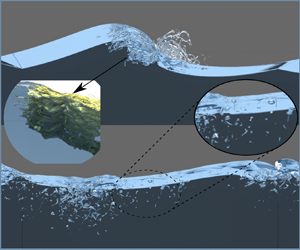
Over the years, a number of review articles and monographs have been published on the subject (Banner & Peregrine Reference Banner and Peregrine1993; Melville Reference Melville1996; Duncan Reference Duncan2001; Babanin Reference Babanin2011; Kiger & Duncan Reference Kiger and Duncan2012; Perlin, Choi & Tian Reference Perlin, Choi and Tian2013; Lubin & Chanson Reference Lubin and Chanson2017; Deike Reference Deike2022), and these works call for more research into nearly every aspect of wave breaking. In open ocean, following wind acts on the water surface leading to the generation of free-surface waves that break when they exceed a limiting steepness, thus injecting momentum and energy into the upper ocean layer. Being the primary mechanism through which energy is transferred from wind to ocean, wave breaking has a significant impact on the global energy balance. In spite of its global influence, the breaking occurs on a relatively small scale, and through the bubble fragmentation and turbulence processes, involves phenomena up to the microscopic scale, thus making the breaking a rather challenging multiscale problem. Garrett, Li & Farmer (Reference Garrett, Li and Farmer2000) suggested that super-Hinze-scale turbulent break-up transfers entrained gas from large to small bubble sizes in the manner of a cascade, and Chan, Johnson & Moin (Reference Chan, Johnson and Moin2021a) provide a theoretical basis for this bubble mass cascade. An example of generation of drops, spray, aerosol and turbulent coherent structures caused by breaking waves is shown in figure 1. The wide range of scales involved in the breaking process is not only in space but also in time. Usually, the breaking occurs in a fraction of the wave period (Bonmarin Reference Bonmarin1989; Rapp & Melville Reference Rapp and Melville1990), which is rather short compared to the time scales at which the wind-generated waves develop as a consequence of the wind forcing and the nonlinear energy transfer across the different wave components (Hasselmann Reference Hasselmann1962, Reference Hasselmann1974). The intermittent and random nature of the breaking phenomenon makes the experimental study in the field very challenging. The breaking is generally identified and characterized based on image analysis and the white-capping coverage (e.g. Sutherland & Melville Reference Sutherland and Melville2015), but such approaches cannot provide any information about the flow and the exchange processes. Much richer is the information that can be obtained beneath the free surface through investigation in the laboratory (e.g. Rapp & Melville Reference Rapp and Melville1990; Duncan et al. Reference Duncan, Qiao, Philomin and Wenz1999; Qiao & Duncan Reference Qiao and Duncan2001; Melville, Veron & White Reference Melville, Veron and White2002; Kimmoun & Branger Reference Kimmoun and Branger2007; Drazen & Melville Reference Drazen and Melville2009; Rojas & Loewen Reference Rojas and Loewen2010; Lubin et al. Reference Lubin, Kimmoun, Véron and Glockner2019). Recent progress on non-intrusive optical techniques has enabled detailed characterization of the flow and the air entrainment process, but due to technical issues caused by light reflection from the bubbles, velocity measurements are available only for a later stage when the large bubbles have degassed (Drazen & Melville Reference Drazen and Melville2009). As a consequence, the phase during which the exchange processes are more relevant remains largely unexplored. Such limitations can be overcome, at least partly, by exploiting the progress of computational methods for the solution of the Navier–Stokes equations in two-phase flows.

Figure 1. Rendering of the breaking wave process, in which bubbles, droplets and sprays are highlighted. The underwater turbulent structures generated by the breaking and the bubble fragmentation process are also shown on the left. Similar structures, not shown for the sake of the clarity, also occur in air.
The numerical investigation of the multiphase flow is very attractive for the perspective of achieving a highly refined description of the flow field in both fluids, thus enabling a quantitative characterization of the exchange processes. Several models have been proposed in the last 25 years, and a comprehensive overview is reported in Mirjalili, Jain & Dodd (Reference Mirjalili, Jain and Dodd2017) and Soligo, Roccon & Soldati (Reference Soligo, Roccon and Soldati2021). Both large-eddy simulations (e.g. Lubin & Glockner Reference Lubin and Glockner2015; Christensen & Rolf Reference Christensen and Rolf2001; Lubin & Chanson Reference Lubin and Chanson2017) and direct numerical simulations (e.g. Deike, Melville & Popinet Reference Deike, Melville and Popinet2016; De Vita, Verzicco & Iafrati Reference De Vita, Verzicco and Iafrati2018) have been used to solve the Navier–Stokes equations. In all cases, the equations are solved for an incompressible fluid with physical properties varying across the air–water interface. Various techniques have been used for the description of the interface dynamics, the most popular being the level-set (Iafrati Reference Iafrati2009), the volume-of-fluid (VOF; Chen et al. Reference Chen, Kharif, Zaleski and Li1999; Deike, Popinet & Melville Reference Deike, Popinet and Melville2015; Chan et al. Reference Chan, Johnson, Moin and Urzay2021b), and hybrids thereof (Wang, Yang & Stern Reference Wang, Yang and Stern2016; Yang, Deng & Shen Reference Yang, Deng and Shen2018).
The first application of a multiphase solver to wave breaking is presented by Chen et al. (Reference Chen, Kharif, Zaleski and Li1999), who simulated the breaking of an artificially steep, third-order Stokes wave in a periodic two-dimensional domain. Owing to problem complexity, the simulation was carried out assuming an unrealistic air–water density ratio of  $1/100$. Despite such a limitation, the study confirmed qualitatively the formation of a plunging jet, the entrainment of air bubbles, generation of vorticity and energy dissipation. Iafrati (Reference Iafrati2009) conducted a similar study by using the actual air–water density ratio $1/800$ and viscosity ratio $\mu _a/\mu _w =0.04$, with Weber number corresponding to about $30$ cm wavelength, and Reynolds number $ {\textit {Re}} = 10\,000$. The study investigated the role of the initial steepness parameter ( $\epsilon$) on the wave evolution and on the breaking process. It was found that breaking occurs for $\epsilon > 0.33$, and it is of spilling type for $\epsilon = 0.35$ and plunging type for $\epsilon \geqslant 0.37$. The analysis focused on energy dissipation, vertical transfer of horizontal momentum, air entrainment and vorticity production. The analysis was continued in Iafrati (Reference Iafrati2011), where the different dissipation mechanisms characterizing spilling and plunging breaking were highlighted. The influence of capillary effects on wave breaking was analysed by Deike et al. (Reference Deike, Popinet and Melville2015). A parametric study in terms of the Bond number and the initial wave steepness was conducted at a relatively high Reynolds number, and the different regimes of gravity-capillary waves, spilling and plunging breaking were distinguished. The formation of aerated vortex filaments in breaking waves was observed by Lubin & Glockner (Reference Lubin and Glockner2015) through three-dimensional numerical simulations. The vortex tubes, identified via the Q-criterion, were found to be rather independent of the breaking intensity and somewhat correlated with striations appearing at the back of the plunging jet, but they were found not to contribute substantially to the dissipation process. Detailed three-dimensional simulations of the two-phase flow and of the fragmentation process occurring during wave breaking events were presented by Deike et al. (Reference Deike, Melville and Popinet2016). A phenomenological model for the bubble size distribution was proposed based on the assumption that the energy dissipated during the breaking scales with the work done against buoyancy force to entrain air. A similar study at higher resolution was carried out by Wang et al. (Reference Wang, Yang and Stern2016), which allowed them to resolve bubbles and droplets at sub-millimetre scale. Probability density functions for the bubble and droplets distributions were derived and compared with the experimental findings of Deane & Stokes (Reference Deane and Stokes2002). Theoretical and numerical investigation of the statistics of the turbulent bubbles break-up cascade at the various stages of wave breaking was presented by Chan et al. (Reference Chan, Johnson and Moin2021a,Reference Chan, Johnson, Moin and Urzayb), who observed that in the early stages the dissipation rate and bubble mass flux are quasi-steady, whereas in the second stage the dissipation rate decays, and the bubble mass flux increases as small and intermediate-sized bubbles become more numerous. Recently, the roles of the Reynolds number and the Bond number (wave scale over the capillary length) on bubble and droplet statistics of strong plunging breakers have been investigated by Mostert, Popinet & Deike (Reference Mostert, Popinet and Deike2022).
In an attempt to induce breaking in a more realistic way, De Vita et al. (Reference De Vita, Verzicco and Iafrati2018) simulated numerically the modulational instability induced by side-band perturbation of a fundamental wave component. The nonlinear interaction of the different wave components causes a downshift of the energy from the fundamental component to the side-bands, which leads to the formation of a rather steep wave. As long as the initial steepness parameter is sufficiently small, the process is reversible; but if, due to the amplification, the maximum wave steepness in the group exceeds a threshold value, then the wave breaks, making the energy transfer from the fundamental to the lower side-band irreversible – see Tulin & Waseda (Reference Tulin and Waseda1999). That study investigated different ways to approach the breaking when varying the initial steepness and the dissipation processes. By singling out the energy contents of the different waves in the group, it was observed that after the breaking, the energy of the most energetic wave in the group decays as  $t^{-1}$, whereas the total energy content of all other waves remains nearly constant. Iafrati, De Vita & Verzicco (Reference Iafrati, De Vita and Verzicco2019) analysed the effect of wind on wave breaking induced via modulational instability, and showed that wind has a stabilizing effect, with breaking occurring at a higher steepness as compared to a no-wind condition.
The results of all the above studies indicate that the fraction of the initial energy content dissipated by the breaking event is nearly independent of the specific conditions, e.g. two-dimensional (2-D) versus three-dimensional (3-D), Bond number, Reynolds number, air–water density ratio. In this study we thus attempt to address in greater detail the dissipation mechanisms during wave breaking events. For that purpose, the breaking of an artificially steep wave (Chen et al. Reference Chen, Kharif, Zaleski and Li1999) is simulated numerically by means of a two-fluid Navier–Stokes solver, considering the actual air–water density ratio, and Weber number corresponding to a  $30$ cm wavelength. Attention is focused primarily on how dissipative processes and associated coherent structures, identified as vortex tubes and vortex sheets, behave at different Reynolds numbers. In the following, the mathematical/numerical set-up is discussed first, and results of validation studies are presented in Appendix A. The model is then applied to simulate wave breaking in a periodic domain, and the analysis is presented in terms of free-surface dynamics, air entrainment and bubble distribution, energy dissipation and coherent structures.
2. Computational set-up
The two-phase flow of air and water taking place during the breaking of a free-surface wave is simulated numerically by a Navier–Stokes solver for a single incompressible fluid with variable physical properties across the interface. The fluids are assumed to be immiscible, and the interface is tracked implicitly by means of an indicator function. Hereafter, the subscript  $1$ is used to denote water, and the subscript $2$ is used for air. The relevant governing equations in non-dimensional form are
 $$\begin{gather} \boldsymbol{\nabla}\boldsymbol{\cdot} \boldsymbol{u} = 0, \end{gather}$$
 $$\begin{gather}\frac{ \partial \boldsymbol{u} } { \partial t} + \boldsymbol{\nabla}\boldsymbol{\cdot} \left(\boldsymbol{uu}\right) = \frac{1}{\rho} \left[ -\boldsymbol{\nabla} p + \frac{1}{{\textit{Re}}}\,\boldsymbol{\nabla} \boldsymbol{\cdot} \left( \mu \left( \boldsymbol{\nabla}\boldsymbol{u}+ \boldsymbol{\nabla}\boldsymbol{u}^{\rm T} \right) \right) + \frac{1}{{\textit{We}}}\, \boldsymbol{f}_{\sigma} \right] - \frac{1}{{\textit{Fr}}}\, \boldsymbol{j}, \end{gather}$$
where  $\boldsymbol {u} = \boldsymbol {u} (\boldsymbol {x}, t)$ is the fluid velocity, $p = p( \boldsymbol {x}, t )$ is the pressure, $\rho = \rho ( \boldsymbol {x}, t )$ is the density, $\mu = \mu ( \boldsymbol {x}, t )$ is the dynamic viscosity, and $\boldsymbol {j}$ is the unit vector oriented upwards. Here, lengths are made non-dimensional with respect to the fundamental wavelength ( $\lambda$), velocities by $\tilde {U} = (g \lambda )^{1/2}$ (with $g$ the gravity acceleration), density and viscosity with the respective values in water, and pressure by $\rho _1 \tilde {U}^2$. Although surface tension acts only at the interface, its effects are modelled as a distributed volumetric force $\boldsymbol {f}_{\sigma } = \boldsymbol {f}_{\sigma } (\boldsymbol {x}, t )$, with
 \begin{equation} \boldsymbol{f}_{\sigma} = k \delta ( \boldsymbol{x} - \boldsymbol{x}_s ) \boldsymbol{n}, \end{equation}
where  $k$ is the local curvature of the interface between the two fluids, $\boldsymbol {n}$ is the unit normal of the interface, and $\delta$ is the Dirac function that localizes the force at interface points $\boldsymbol {x}_s$ (Tryggvason, Scardovelli & Zaleski Reference Tryggvason, Scardovelli and Zaleski2011). In (2.2), $ {\textit {Re}}$, $ {\textit {We}}$ and $ {\textit {Fr}}$ are, respectively, the Reynolds, Weber and Froude numbers, defined as
 \begin{equation} {\textit{Re}} = \frac{\tilde{U} \lambda \rho_1} {\mu_1}, \quad {\textit{We}} = \frac{\rho_1 \tilde{U}^2 \lambda }{ \sigma}, \quad {\textit{Fr}} = \frac{\tilde{U}^2}{g \lambda} ,\end{equation}
where  $\sigma$ is the surface tension coefficient, here assumed to be constant.
The Navier–Stokes equations are solved with a classical projection method in which the momentum equation is advanced in time by neglecting the pressure gradient. Hence the pressure gradient is determined by enforcing the continuity equation, and it is added to the intermediate velocity field in a correction step (Chorin Reference Chorin1968; Orlandi Reference Orlandi2012). Time integration is carried out by means of the Adams–Bashforth explicit scheme for the convective terms and for the off-diagonal part of the viscous terms, and the Crank–Nicolson scheme for the diagonal diffusion terms. Hence (2.2) becomes, in discrete form,
 \begin{align} \frac{\boldsymbol{u}^{n+1} - \boldsymbol{u}^n}{\Delta t} &={-}\frac{1}{\rho^{n+{1}/{2}}}\,\boldsymbol{\nabla}_h p - \left( \frac{3}{2}\, \boldsymbol{N}^n_h - \frac{1}{2}\,\boldsymbol{N}^{n-1}_h \right) \nonumber\\ &\quad + \frac{1}{2 \rho^{n+{1}/{2}}} \left( \boldsymbol{D}^n_h + \boldsymbol{D}^{n+1}_h \right) + \frac{1}{\rho^{n+{1}/{2}}}\, \boldsymbol{f}^n , \end{align}
where  $\Delta t$ is the time step. The superscript $n$ denotes quantities evaluated at the beginning of the step, and $n + 1$ identifies the end of the step. As suggested by Popinet (Reference Popinet2009), the material properties (viscosity and density) in the previous equation are evaluated by advancing the respective transport equation at staggered times (see § 2.1). The notation $\boldsymbol {N}_h$ and $\boldsymbol {D}_h$ is used to denote numerical approximations of the advection and diffusion terms, and $\boldsymbol {f}$ includes gravity and surface tension forces. Similarly, $\boldsymbol {\nabla }_h$ stands for a numerical approximation of the gradient operator. The momentum equation (2.5) is complemented with the divergence-free conditions
 \begin{equation} \boldsymbol{\nabla}_h \boldsymbol{\cdot} \boldsymbol{u}^{n+1} = 0 . \end{equation}
The momentum equation (2.5) is solved in two steps. In the predictor step, a temporary velocity field ( $\boldsymbol {u}^*$) is determined by ignoring the effect of the pressure:
 \begin{equation} \frac{\boldsymbol{u}^* - \boldsymbol{u}^n}{\Delta t} ={-} \left( \frac{3}{2}\,\boldsymbol{N}^n_h - \frac{1}{2}\,\boldsymbol{N}^{n-1}_h \right) + \frac{1}{2 \rho^{n+{1}/{2}}\,{\textit{Re}}} \left( \boldsymbol{D}^n_h + \boldsymbol{D}^*_h \right) + \frac{1}{\rho^{n+{1}/{2}}}\, \boldsymbol{f}^n . \end{equation}
In the correction step, the pressure gradient is added to the temporary velocity field to yield the velocity field at the new time step:
 \begin{equation} \frac{\boldsymbol{u}^{n+1} - \boldsymbol{u}^*}{\Delta t} ={-}\frac{1} {\rho^{n+{1}/{2}}}\,\boldsymbol{\nabla}_h p . \end{equation}
Adding (2.7) and (2.8) yields (2.5) exactly. Taking the discrete divergence of (2.8) and using (2.6) to eliminate  $\boldsymbol {u}^{n+1}$, a Poisson equation for the pressure is obtained:
 \begin{equation} \boldsymbol{\nabla}_h \boldsymbol{\cdot} \left( \frac{1}{\rho^{n+{1}/{2}}}\,\boldsymbol{\nabla}_h p \right) = \frac{1}{\Delta t}\,\boldsymbol{\nabla}_h \boldsymbol{\cdot} \boldsymbol{u}^* . \end{equation}
Once the pressure is solved for, (2.8) is used to determine the velocity field at time  $n + 1$. The convective terms and the off-diagonal part of the viscous operator are rearranged as
 \begin{equation} \left.\begin{gathered} \boldsymbol{N}^n_h = \boldsymbol{\nabla}_h \boldsymbol{\cdot} \boldsymbol{u}^n \boldsymbol{u}^n - \frac{1}{\rho^{n+{1}/{2}}\,{\textit{Re}}}\,\boldsymbol{\nabla}_h \boldsymbol{\cdot} \left( \mu^{n+{1}/{2}}\,\boldsymbol{\nabla} \boldsymbol{u}^{{\rm T}\,n} \right), \\ \boldsymbol{N}^{n-1}_h = \boldsymbol{\nabla}_h \boldsymbol{\cdot} \boldsymbol{u}^{n-1} \boldsymbol{u}^{n-1} - \frac{1}{\rho^{n+{1}/{2}}\, {\textit{Re}}}\,\boldsymbol{\nabla}_h \boldsymbol{\cdot} \left( \mu^{n+{1}/{2}}\,\boldsymbol{\nabla} \boldsymbol{u}^{{\rm T}\,n-1} \right) , \end{gathered}\right\} \end{equation}
whereas the diagonal part of the viscous term becomes
 \begin{equation} \boldsymbol{D}_h^n = \boldsymbol{\nabla}_h \boldsymbol{\cdot} \left( \mu^{n+{1}/{2}}\,\boldsymbol{\nabla} \boldsymbol{u}^n \right), \qquad \boldsymbol{D}_h^* = \boldsymbol{\nabla}_h \boldsymbol{\cdot} \left( \mu^{n+{1}/{2}}\,\boldsymbol{\nabla} \boldsymbol{u}^* \right) , \end{equation}
which, by defining  $\delta \boldsymbol {u}^n = \boldsymbol {u}^* - \boldsymbol {u}^n$, allows us to reformulate the problem in delta form,
 \begin{align} \boldsymbol{D}_h^n + \boldsymbol{D}_h^* &= \boldsymbol{\nabla}_h \boldsymbol{\cdot} \left( \mu^{n+{1}/{2}} \left( \boldsymbol{\nabla}_h \boldsymbol{u}^n + \boldsymbol{\nabla}_h \left( \delta \boldsymbol{u}^n + \boldsymbol{u}^n \right)\right) \right)\nonumber\\ &= \boldsymbol{\nabla}_h \boldsymbol{\cdot} \left( \mu^{n+{1}/{2}} \left( \boldsymbol{\nabla}_h \delta \boldsymbol{u}^n + 2 \left( \boldsymbol{\nabla}_h \boldsymbol{u}^n \right) \right) \right). \end{align}
Starting from (2.7), it follows that
 \begin{align} \frac{ \delta \boldsymbol{u}^n}{ \Delta t} - \frac{1}{2 \rho^{n+ 1/2}\,{\textit{Re}}}\,\boldsymbol{\nabla}_h \boldsymbol{\cdot} \left( \mu ^{n+{1}/{2}}\, \boldsymbol{\nabla}_h \delta \boldsymbol{u}^n \right) &={-} \left( \frac{3}{2}\,\boldsymbol{N}^n_h - \frac{1}{2}\,\boldsymbol{N}^{n-1}_h \right) + \frac{1}{\rho^{n+{1}/{2}}\,{\textit{Re}} }\,\boldsymbol{D}_h^n \nonumber\\ &\quad+ \frac{1}{ \rho^{n+{1}/{2}}\,{\textit{We}}}\,\boldsymbol{f}_{\sigma}^n - \frac{1}{ {\textit{Fr}}}\,\boldsymbol{j} . \end{align}
If the left-hand side of the above equation is discretized using second-order finite differences, and the right-hand side is denoted as  $\textrm {RHS}_i$, where $i$ is the $i$th component, then it is found that
 \begin{equation} \left[ 1 - \Delta t \left( L_{i1} - L_{i2} - L_{i3} \right) \right] \delta u_i = {\rm RHS}_i , \end{equation}
to which the approximate factorization is applied, resulting in
 \begin{equation} \left( 1 - A_{i1} \right) \left( 1 - A_{i2} \right) \left( 1 - A_{i3} \right) \delta u_i = {\rm RHS}_i, \end{equation}
where  $A_{ij} = \Delta t\,L_{ij}$, and
 \begin{equation} \left.\begin{gathered} A_{i1} = \frac{1}{2 \rho^{n+{1}/{2}} }\,\frac{\partial}{\partial x_1} \left( \mu^{n+{1}/{2}}\, \frac{\partial}{\partial x_1} \right), \\ A_{i2} = \frac{1}{2 \rho^{n+{1}/{2}} }\,\frac{\partial}{\partial x_2} \left( \mu^{n+{1}/{2}}\, \frac{\partial}{\partial x_2} \right), \\ A_{i3} = \frac{1}{2 \rho^{n+{1}/{2}} }\,\frac{\partial}{\partial x_3} \left( \mu^{n+{1}/{2}}\,\frac{\partial}{\partial x_3} \right) . \end{gathered}\right\} \end{equation}
The left-hand side of (2.15) can be shown to be a third-order-accurate approximation of the large sparse matrix at the left-hand side of (2.14) (Orlandi Reference Orlandi2012). Equation (2.15) can then be solved by sequential application of algorithms for solving tridiagonal linear systems:
 \begin{equation} \left.\begin{gathered} \left( 1 - A_{i1} \right) \delta u_i ^{**} = {\rm RHS}_i, \\ \left( 1 - A_{i3} \right) \delta u_i ^{*} = \delta u_i ^{**}, \\ \left( 1 - A_{i2} \right) \delta u_i ^n = \delta u_i ^{*} , \end{gathered}\right\} \end{equation}
where  $\delta u^{**}$ and $\delta u^*$ denote time increments at fictitious intermediate stages.
2.1. VOF formulation
Since fluids are assumed to be immiscible, the advection of the material interface is carried out by means of an algebraic VOF method. The numerical scheme for the advection is based on a novel Courant–Friedrichs–Lewy-dependent flux limiter whereby the classical total-variation-diminishing (TVD) bounds are exceeded, thus enabling efficient and improved representation of binary functions (Pirozzoli, Di Giorgio & Iafrati Reference Pirozzoli, Di Giorgio and Iafrati2019). The method yields perfectly crisp interfaces with very limited numerical atomization (flotsam and jetsam). Let  $\chi$ be a passive tracer advected by a continuous divergence-free velocity field $\boldsymbol {u}$, which satisfies the passive transport equation
 \begin{equation} \frac{\partial \chi}{\partial t} + \boldsymbol{\nabla}\boldsymbol{\cdot} (\chi {\boldsymbol{u}}) = 0. \end{equation}
For the problem under scrutiny here,  $\chi$ is either $1$ or $0$, which is the case of two immiscible fluids. In the VOF method, a colour function is introduced to approximate the cell average of $\chi$, which in the illustrative case of one space dimension is defined as
 \begin{equation} C_i = \frac 1{\Delta x_i} \int_{x_{i-1/2}}^{x_{i+1/2}} \chi (x,t^n)\, \mathrm{d} x , \end{equation}
where  $\Delta x_i = x_{i+1/2}-x_{i-1/2}$ is the cell size. Equation (2.18) is then discretized in time yielding
 \begin{equation} C_i^{n+1/2} = C_i^{n- 1/2} - \frac{1}{\Delta x_i} \left( \hat{f}_{i+1/2} - \hat{f}_{i-1/2} \right) , \end{equation}
where the numerical flux  $\hat {f}_{i+1/2}$ is an approximation for the amount of $\chi$ transported through the cell interface $x_{i+1/2}$ during the time interval $(t^{n-1/2}, t^{n+1/2})$. This is determined by assuming piecewise linear reconstruction within each cell, namely
 \begin{equation} C_{i}(x) = C^n_{i} + s_{i} (x-x_{i}), \end{equation}
with slope  $s_i$ selected so as to prevent the occurrence of overshoots/undershoots by enforcing the TVD constraints (Sweby Reference Sweby1984)
 \begin{equation} s_i = \frac{1}{\Delta x_{i}}\,\varphi(\theta_{i+1/2})\,\delta C_{i+1/2} , \end{equation}
where  $\delta C_{i+1/2} = C_{i+1}-C_i$, $\theta _{i+1/2}=\delta C_{i-1/2}/\delta C_{i+1/2}$. Suitable choice of the slope limiter function $\varphi$ is found to provide crisp resolution of contact discontinuities (with 2–3 grid points), and absence of spurious flotsam–jetsam as in early implementations of the TVD idea (Noh & Woodward Reference Noh and Woodward1976; Hirt & Nichols Reference Hirt and Nichols1981). Details of the algorithm are provided in the original reference, Pirozzoli et al. (Reference Pirozzoli, Di Giorgio and Iafrati2019). After computing the colour function $C$, density and viscosity are determined from
 \begin{equation} \rho = \tilde{C} + \frac{\rho_2}{\rho_1} \left( 1 - \tilde{C} \right), \quad \mu = \tilde{C} + \frac{\mu_2}{\mu_1} \left( 1 - \tilde{C} \right) , \end{equation}
where  $\tilde {C}$ is a smoothed version of the colour function, evaluated by averaging $C$ over 27 neighbouring cells (Popinet Reference Popinet2009; Tryggvason et al. Reference Tryggvason, Scardovelli and Zaleski2011).
2.2. Spatial discretization
The momentum equations are discretized in the finite-difference framework with a staggered grid layout, where the pressure, the colour function and the material properties are defined at the cell centres, whereas the velocity components are stored at the middle of the cell faces (Harlow & Welch Reference Harlow and Welch1965). The right-hand side of (2.13) is rewritten in order to cast convective and diffusive terms in a more canonical form:
 \begin{align} {\rm RHS} & ={-}\left( \frac{3}{2}\, \boldsymbol{H}^n_h-\frac{1}{2}\,\boldsymbol{H}^{n-1}_h \right) + \frac{1}{\rho^{n+{1}/{2}}\,{\textit{Re}} } \left[ \boldsymbol{\varSigma}_h^n + \frac{1}{2} \left( \boldsymbol{\nabla}_h \boldsymbol{u}^{{\rm T},n} - \boldsymbol{\nabla}_h \boldsymbol{u}^{{\rm T},n-1} \right) \boldsymbol{\nabla}_h \mu^{n+{1}/{2}} \right] \nonumber\\ &\quad + \frac{1}{ \rho^{n+{1}/{2}}\,{\textit{We}}}\,\boldsymbol{f}_{\sigma}^n - \frac{1}{ \rho^{n+{1}/{2}}\,{\textit{Fr}}}\,\boldsymbol{j} , \end{align}
where  $\boldsymbol {H}_h$ and $\boldsymbol {\varSigma }_h$ denote, respectively, convective and viscous terms. Terms associated with variation of viscosity appear in this case, which are rearranged as
 \begin{align} &\frac{1}{\rho^{n+{1}/{2}}\,{\textit{Re}}} \left[ \frac{3}{2}\, \boldsymbol{\nabla}_h \boldsymbol{\cdot} \left( \mu^{n+{1}/{2}}\,\boldsymbol{\nabla} {\boldsymbol{u}}^{{\rm T},n} \right) - \frac{1}{2}\,\boldsymbol{\nabla}_h \left( \mu^{n+{1}/{2}}\,\boldsymbol{\nabla} {\boldsymbol{u}}^{{\rm T},n-1} \right) \right] \nonumber\\ &\quad = \frac{1}{\rho^{n+{1}/{2}}\,{\textit{Re}}} \left[ \boldsymbol{\nabla}_h \boldsymbol{\cdot} \left( \mu^{n+{1}/{2}}\,\boldsymbol{\nabla}{\boldsymbol{u}}^{{\rm T},n} \right) + \frac{1}{2} \left( \boldsymbol{\nabla}_h \boldsymbol{\cdot} \left( \mu^{n+{1}/{2}}\,\boldsymbol{\nabla} {\boldsymbol{u}}^{{\rm T},n} \right) - \boldsymbol{\nabla}_h \boldsymbol{\cdot} \left(\mu^{n+{1}/{2}}\,\boldsymbol{\nabla} {\boldsymbol{u}}^{{\rm T},n-1}\right)\right)\right] , \end{align}
and exploiting incompressibility, one has
 \begin{align} \boldsymbol{\nabla}_h \boldsymbol{\cdot} \left( \mu^{n+{1}/{2}}\,\boldsymbol{\nabla} {\boldsymbol{u}}^{{\rm T},n} \right) &= \boldsymbol{\nabla}_h \boldsymbol{u}^{{\rm T},n}\,\boldsymbol{\nabla}_h \mu^{n+{1}/{2}} + \mu^{n+{1}/{2}}\,\boldsymbol{\nabla}_h \boldsymbol{\cdot} \boldsymbol{\nabla}_h {\boldsymbol{u}}^{{\rm T},n} \nonumber\\ &= \boldsymbol{\nabla}_h {\boldsymbol{u}}^{{\rm T},n}\,\boldsymbol{\nabla}_h \mu^{n+{1}/{2}} + \mu^{n+{1}/{2}}\,\boldsymbol{\nabla}_h \left( \boldsymbol{\nabla}_h \boldsymbol{\cdot} {\boldsymbol{u}} \right) \nonumber\\ &= \boldsymbol{\nabla}_h {\boldsymbol{u}}^{{\rm T},n}\,\boldsymbol{\nabla}_h \mu^{n+{1}/{2}} . \end{align}
For the convective terms, defined as
 \begin{equation} \boldsymbol{H}^n_h = \boldsymbol{\nabla}_h \boldsymbol{\cdot} ( \boldsymbol{u}^n \boldsymbol{u}^n ) , \quad \boldsymbol{H}^{n-1}_h = \boldsymbol{\nabla}_h \boldsymbol{\cdot} ( \boldsymbol{u}^{n-1} \boldsymbol{u}^{n-1} ) , \end{equation}
a centred second-order discretization is used (e.g. Harlow & Welch Reference Harlow and Welch1965; Orlandi Reference Orlandi2012), which is generally best suitable for fully resolved flows, yielding discrete preservation of the total kinetic energy in the case of uniform density. For the diffusive terms, which are written as
 \begin{equation} \boldsymbol{\varSigma}_h^n = \boldsymbol{\nabla}_h \boldsymbol{\cdot} \mu^{n+{1}/{2}} \left( \boldsymbol{\nabla}_h \boldsymbol{u}^{n} + \boldsymbol{\nabla}_h \boldsymbol{u}^{{\rm T},n} \right), \end{equation}
a standard second-order central discretization is used (Tryggvason et al. Reference Tryggvason, Scardovelli and Zaleski2011).
The last step concerns the solution of the Poisson equation (2.9) for the corrective pressure, which is also the most expensive part in multiphase flow solvers in terms of computational effort. The Poisson equation is discretized by a finite-difference scheme with a staggered Cartesian mesh. The resulting sparse linear system is solved by iterative methods. In particular, the HYPRE library (Falgout & Yang Reference Falgout and Yang2002) is found to be very efficient in massively parallel computations. Both geometric multigrids and the Krylov methods have been tested, the latter proving to be more robust in the presence of complicated flow topologies.
2.3. Surface tension
The modelling of surface tension effects is the most peculiar and critical aspect when developing a multiphase flow solver. Use of the VOF method, which has advantages in terms of mass conservation, has some drawbacks when the curvature on the interface has to be estimated, which is necessary for the determination of surface tension. In this work, the continuum surface force method (Brackbill, Kothe & Zemach Reference Brackbill, Kothe and Zemach1992) is used to determine the equivalent local body force, whereas the interface curvature is evaluated through the height function technique (Cummins, Francois & Kothe Reference Cummins, Francois and Kothe2005; Francois et al. Reference Francois, Cummins, Dendy, Kothe, Sicilian and Williams2006; Hernández et al. Reference Hernández, López, Gómez, Zanzi and Faura2008; López & Hernández Reference López and Hernández2010; Popinet Reference Popinet2009; Aniszewski et al. Reference Aniszewski2021)). The height function method is known to work well as long as the height function is within the cell dimension (Cummins et al. Reference Cummins, Francois and Kothe2005). At points where this condition is not met, the interface curvature is estimated based on the gradient of the interface normal vector (Goldman Reference Goldman2005):
 \begin{equation} k = \frac{\boldsymbol{\nabla} \tilde{C} \ast H ( \tilde{C} ) \ast \boldsymbol{\nabla} \tilde{C}^{\rm T} - | \boldsymbol{\nabla} \tilde{C} |^2 \,{\rm Tr}\bigl(H ( \tilde{C} ) \bigr)} {2 | \boldsymbol{\nabla} \tilde{C} |^3 }, \end{equation}
where  $\boldsymbol {\nabla } \tilde {C}$ and $H( \tilde {C} )$ are, respectively, the gradient and the Hessian of the smoothed colour function. The first- and second-order derivatives of the colour function field ( ${\partial \tilde {C}}/{\partial x_i}$ and ${\partial ^2 \tilde {C}}/{\partial x_i\, \partial x_j }$) are approximated using the least-squares method (Ding et al. Reference Ding, Shu, Yeo and Xu2004). A detailed verification and validation study of the solver is reported in Appendix A.
3. Numerical simulation of wave breaking
3.1. Flow cases
Results of numerical simulations of wave breaking are hereafter reported for the idealized case of a wave train with assumed periodicity in the streamwise and spanwise directions (see figure 2). The initial free-surface elevation  $\eta (x,z)$ is assigned as in Iafrati (Reference Iafrati2009), Chen et al. (Reference Chen, Kharif, Zaleski and Li1999), Deike et al. (Reference Deike, Popinet and Melville2015, Reference Deike, Melville and Popinet2016) and Wang et al. (Reference Wang, Yang and Stern2016), that is,
 \begin{equation} \eta (x,z) = \frac{\epsilon}{2 {\rm \pi}} \left( \cos ( k \left(x - r(z)\,\Delta x \right) ) + \frac{1}{2} \epsilon \cos ( 2 k \left(x - r(z)\,\Delta x \right) ) + \frac{3}{8} \epsilon^2 \cos ( 3 k \left(x - r(z)\,\Delta x \right) ) \right), \end{equation}
where  $\epsilon = a k$ is the initial wave steepness, $a$ is the wave amplitude, $k = 2 {\rm \pi}$ is the fundamental wavenumber, and the period of the fundamental wave component is $T = \sqrt {2 {\rm \pi}} \approx 2.5$. A small perturbation is introduced in the initial wave profile in the form of a random shift by a fraction ( $0 \leqslant r(z) \leqslant 1$) of the grid cell size. The corresponding initial velocity field in water is derived from potential flow theory:
 $$\begin{gather} u(x,y,z) = \varOmega\,\frac{\epsilon}{k} \exp ( k y ) \cos ( k \left(x - r(z)\,\Delta x \right) ), \quad \forall \, y < \eta(x,z), \end{gather}$$
 $$\begin{gather}v(x,y,z)= \varOmega\,\frac{\epsilon}{k} \exp ( k y ) \sin ( k \left(x - r(z)\, \Delta x \right) ), \quad \forall \, y < \eta(x,z), \end{gather}$$
where  $\varOmega = \sqrt {k / {\textit {Fr}}\,( 1 + \epsilon ^2 ) }$ accounts for nonlinear corrections (Whitham Reference Whitham1974). No-slip boundary conditions are assigned at the top and bottom boundaries. At the beginning of the simulation, the fluid in the air domain, i.e. $y > \eta (x,z)$, is assumed to be at rest. As soon as the simulation starts, the solution of the Poisson equation enforces the continuity of the velocity field, therefore the velocity in air is initialized as a divergence-free velocity field satisfying the continuity of the normal velocity at the interface. Later on, motion in air is induced by momentum exchange occurring at the interface due to the normal and tangential stresses. As the water depth is of the same order as the fundamental wavelength, wave propagation can be regarded to be of deep-water type, and the presence of the bottom does not affect the evolution of the breaking process substantially (Chen et al. Reference Chen, Kharif, Zaleski and Li1999). For similar reasons, at such a wavelength/depth ratio, the energy loss by bottom friction is essentially negligible (Lighthill Reference Lighthill1978). Two- and three-dimensional numerical simulations have been carried out for different Reynolds numbers, but in all cases it is assumed that
 \begin{equation} {\textit{We}} = \frac{\rho_1 \tilde{U}^2 \lambda}{\sigma} = \frac{\rho_1 g \lambda^2}{\sigma} = 12\,262.5 . \end{equation}
Assuming the surface tension coefficient to be  $0.072\ \textrm {N}\ \textrm {m}^{-1}$, the chosen Weber number corresponds to water waves with about $30$ cm fundamental wavelength. At such a wavelength, the Reynolds number is
 \begin{equation} {\textit{Re}} = \frac{\rho_1 \tilde{U} \lambda}{\mu_1}= \frac{\rho_1 g^{1/2} \lambda^{3/2}}{\mu_1} \approx 5.1 \times 10^5 . \end{equation}
Numerical simulations at such a Reynolds number would require a considerable computational effort for all the relevant scales of the flow to be fully resolved. In order to minimize artefacts due to lack of sufficient resolution, simulations have been conducted at  $ {\textit {Re}}=10\,000$ and $40\,000$. Despite this limitation, viscous effects may be regarded as representative of full-scale conditions, while providing accurate and energy-preserving solutions. In all cases, the density and viscosity ratios are assumed to be $\rho _1/\rho _2 = 800$ and $\mu _1/\mu _2 = 55$, hence representative of the real air–water system. The flow parameters for the various simulations performed are listed in table 1. The computational domain is one fundamental wavelength long (streamwise direction), two fundamental wavelengths high (vertical direction), and for 3-D simulations, one-half fundamental wavelength wide (spanwise direction), namely $x \in [-0.5 , 0.5 ]$, $y \in [-1, 1 ]$, $z \in [-0.25 , 0.25 ]$. Each 3-D simulation has been carried out at two grid resolutions, in order to gain information about grid sensitivity. In all cases, the grid cells are uniformly spaced in the $x$- and $z$-directions, whereas in the vertical direction, cells are clustered about the still-water level in order to achieve better resolution around the interface. In particular, the grid size is kept uniform for $-0.25 \leqslant y \leqslant 0.25$, and progressively increased moving away from the centre of the domain (Orlandi Reference Orlandi2012, § 2.2.3c). Assuming $\lambda =30$ cm, the resulting grid spacing in the well-resolved zone is about $0.6$ mm in the coarse-mesh simulations (as in Chen et al. Reference Chen, Kharif, Zaleski and Li1999), and $0.3$ mm in the fine-mesh simulations.

Figure 2. Sketch of the computational set-up for the study of wave breaking: no-slip boundary conditions are assigned at the top and bottom boundaries, whereas periodic boundary conditions are assigned in the streamwise ( $x$) and spanwise ( $z$) directions.
Table 1. List of simulations performed. For all cases,  $ {\textit {We}} = 12\,262.5$. Columns show the simulation identifier, the number of cells used, the domain size in the streamwise, vertical and spanwise directions, the initial steepness parameter, and the Reynolds number of the liquid phase.

Particularly at the shortest scales, the dynamics of the breaking is strongly affected by surface tension (Duncan Reference Duncan2001). An illustration of the various stages of the breaking process is provided in figure 3, where kinetic energy and instantaneous streamtraces are shown. Starting from the initial conditions (figure 3a), the onset of the breaking occurs at the time instant at which for the first time a portion of the air–water interface becomes vertical (figure 3b). Next, curling of the crest and plunging onto the forward face are displayed in figure 3(c), which shows the impact of the water jet and subsequent air entrainment. Finally, figure 3(d) shows the splash-up and successive impacts on the free surface, and resulting air entrainment (Kiger & Duncan Reference Kiger and Duncan2012). The simulations are advanced in time up to  $t/T=2.8$, at which time most energy has been dissipated, and effects of spurious streamwise periodicity are still small.

Figure 3. Air entrainment in a plunging breaker: slices of the 3D1E4c flow case are reported, showing contours of kinetic energy, and instantaneous streamtraces: (a) initial condition,  $t/T = 0.0$; (b) breaking inception, $t/T = 0.26$; (c) initial jet impact, $t/T = 0.38$; (d) backward-splash entrainment, $t/T = 0.84$.
3.2. Influence of initial conditions and grid size
In order to derive a quantitative estimate of the uncertainty in the numerical results, for the 2-D case, five repetitions of the same simulation have been carried out by imparting small random perturbations of the initial wave profile (3.1). This is to mimic what usually happens in experiments where, due to the residual turbulence level and/or small perturbations in the initial free-surface profile, differences in the breaking dynamics occur, although the main features are quite repeatable. In figure 4, the time histories of the total mechanical energy for the various simulations are reported. Up to onset of breaking, the results are perfectly overlapping. However, when breaking initiates, minor changes in the air entrainment and in the bubble fragmentation process caused by the different initial shifts lead to progressive divergence in the behaviour of the total energy. At the end of the simulation, the maximum scatter across cases is about  $10-15\,\%$ of the initial energy content. This issue should be kept in mind when comparing different simulations. The results of 2-D simulations with initially perturbed state are then used to extract an ensemble average of the volume fraction and associated density and viscosity fields. For that purpose, an intermittency coefficient (Brocchini & Peregrine Reference Brocchini and Peregrine2001)
 \begin{equation} \bar{C}( \boldsymbol{x},t ) = \frac{ \sum^N_i C_i ( \boldsymbol{x}, t ) }{ N } \end{equation}
is determined as an average of the local volume fraction over  $N= 5$ simulations with different initial conditions, as shown in figure 5. The time evolution confirms that all computed solutions are well overlapping up to the breaking onset, also in terms of the free-surface profile. As soon as the water jet plunges onto the free surface, larger differences emerge in the size and distributions of the entrapped bubbles, thus leading to much wider scatter. Differences are originated by strong nonlinearities in the flow triggered by changes associated with use of a discrete grid to describe the fragmentation and reconnection processes of the interface. At a later stage, the large air cavity that forms breaks down into smaller cavities that subsequently rise up and emerge from the water, thus the intermittency region shrinks, while remaining larger than the grid cell.

Figure 4. Time histories of total energy for 2-D simulations with initial steepness  $\epsilon = 0.5$, with different initial perturbations.

Figure 5. Contours of ensemble-averaged volume fraction of 2-D simulations with perturbed initial conditions at different times, (a)  $t/T = 0.4$, (b) $t/T = 0.8$, (c) $t/T = 1.2$, (d) $t/T = 1.6$, (e) $t/T = 2.0$, and (f) $t/T = 2.4$.
The effect of the grid resolution is analysed in the 3-D flow cases. In order to test the capability of the computational model to resolve all the relevant scales responsible for energy dissipation, a comparison between the time history of the total energy ( $E_{tot}$) obtained from the simulations on coarse and fine meshes is displayed in figure 6. The total energy is here defined as
 \begin{align} E_{tot} = \underbrace{ \int_{V} \frac{1}{2}\,\rho ( u^2 + v^2 +w ^2 )\,\mathrm{d} V }_{\text{kinetic energy}} + \underbrace{\int_{V} \rho\,g (y + d/2) \,\mathrm{d} V }_{\text{potential energy}} + \underbrace{\frac{1} {We}\, ( \mathcal{S} -1 ) }_{\text{surface tension potential energy}} , \end{align}
where the first term on the right-hand side is the total kinetic energy, the second term is the potential energy, with  $d$ the water depth, and the last term is the surface tension potential energy, with $\mathcal {S}$ the surface area of the interface. No significant difference is observed between coarse and fine simulations during the pre-breaking phase. Once the breaking starts, small differences develop, which, nevertheless, are within the inherent uncertainty of the simulations as discussed previously in the 2-D case.

Figure 6. Evolution of total energy as obtained from 3-D simulations of wave breaking with  $\epsilon = 0.5$. Results are shown for (a) $ {\textit {Re}}=10\,000$, and (b) $ {\textit {Re}}=40\,000$.
3.3. Energy budgets
Starting from the momentum and continuity equations, the following integral budget equation can be derived:
 \begin{align} \frac{{\rm d}}{{\rm d}t} \underbrace{ \int_V \left(\rho\,\frac{u^2}{2} + \rho g y\right) \mathrm{d} V}_{\text{total energy}} &={-} \underbrace{ \oint_{\partial V} \left( p + \rho\,\frac{u^2}{2} + \rho g y \right) \boldsymbol{u} \boldsymbol{\cdot} \boldsymbol{n} \, \mathrm{d} S }_{\text{boundary energy flux}} + \underbrace{ \oint_{\partial V} \left( \varSigma \boldsymbol{\cdot} \boldsymbol{u} \right) \boldsymbol{\cdot} \boldsymbol{n} \, \mathrm{d} S }_{\text{work of surface tension forces}} \nonumber\\ &\quad - \underbrace{ \int_V \boldsymbol{\varSigma} : \boldsymbol{\nabla} \boldsymbol{u} \, \mathrm{d} V }_{ \text{viscous dissipation} } + \underbrace{ \int_V \boldsymbol{u} \boldsymbol{\cdot} \boldsymbol{f}_{\sigma} \, \mathrm{d} V }_{\text{ work of tension forces} }, \end{align}
where surface integrals over the domain boundaries vanish due to the periodicity in the streamwise and spanwise directions, and to the no-slip boundary condition at the bottom and top walls. It is important to note that the above equations apply in continuous form, but they are not valid rigorously in discrete form, depending on the numerical scheme and grid size. The discretization scheme adopted in the present model for the momentum equation conserves the total energy also in discrete form in the case of a single fluid (Orlandi Reference Orlandi2012). However, the conservation properties are not guaranteed in case of multiphase flows due to the variation of the fluid properties, and of the density in particular. In figure 7, the time histories of the total mechanical energy for the various simulations are compared with the time integrals of the sum of the viscous dissipation and surface tension work terms. The results highlight satisfactory agreement between the energy decay and the total dissipation, which, as expected, improves for the case of fine grid computations. Differences are minor prior to breaking, and become more significant once breaking starts. After the start of the breaking occurring at about  $t/T \approx 0.5$, the air–water interface increases in size owing to air entrainment and bubble fragmentation, but in spite of that, the energy conservation properties of the discrete form of the convective terms and of the approximate representation of the surface tension are confirmed.

Figure 7. Time histories of total mechanical energy (purple line with solid square symbols) and of the time integral of the sum of viscous dissipation and surface tension work (green line with open circles) for 3-D simulations of wave breaking with initial steepness  $\epsilon = 0.5$: (a) $ {\textit {Re}}=10\,000$, coarse grid (3D1E4c); (b) $ {\textit {Re}}=10\,000$, fine grid (3D1E4f); (c) $ {\textit {Re}}=40\,000$, coarse grid (3D4E4c); (d) $ {\textit {Re}}=40\,000$, fine grid (3D4E4f).
3.4. Role of breaking in energy dissipation
The time histories of kinetic, potential, surface tension and total energies during the breaking process are shown in figure 8 for  $ {\textit {Re}}=10\,000$ and $40\,000$, limited to fine grid cases. In the early stages, the total energy follows the theoretical decay rate estimated by Landau & Lifschitz (Reference Landau and Lifshitz1987), whereas a sharp increase of energy dissipation occurs shortly after the onset of breaking. The time histories of the kinetic and potential energy contributions are characterized by oscillatory behaviours with opposite phases, associated with the bound wave component. As long as the wave is regular, the two contributions are balanced, and their sum remains constant. During the breaking stage, owing to plunging of the water jet with subsequent air entrainment and bubble fragmentation, large vortical structures develop that yield an increase of kinetic energy as compared to potential energy. The time history of the total energy shows that most dissipation occurs within about one wave period, in agreement with results of previous authors (Chen et al. Reference Chen, Kharif, Zaleski and Li1999; Iafrati Reference Iafrati2009; Deike et al. Reference Deike, Popinet and Melville2015, Reference Deike, Melville and Popinet2016; Wang et al. Reference Wang, Yang and Stern2016). As discussed by Iafrati (Reference Iafrati2011), most dissipation is associated with the formation of small-scale bubbles, which increase the size of the air–water interface and thus the surface tension contribution, and is accompanied with severe velocity gradients, mainly concentrated into vortex sheets (see below). The results of simulations at the two Reynolds numbers are quite similar, except for small differences in the dissipated energy fraction. Besides uncertainties discussed previously, part of this difference is associated with the different amount of the energy fraction that would be dissipated in the absence of breaking, as suggested by the theoretical estimates (thin black lines in figure 8). The above results corroborate findings made in previous studies (e.g. Lubin et al. Reference Lubin, Vincent, Abadie and Caltagirone2006; Iafrati Reference Iafrati2009; Deike et al. Reference Deike, Popinet and Melville2015), which showed that the dissipated energy fraction does not depend much on the Reynolds number, or on dimensionality.

Figure 8. Time histories of kinetic energy ( $E_k$), potential energy ( $E_p$), surface tension energy ( $E_s$) and total energy ( $E_{tot}$) of water for 3-D wave breaking with initial steepness $\epsilon = 0.5$. Here, $E_0$ is the initial total energy, and $T$ is the wave period. The solid black line represents the theoretical linear viscous dissipation $E/E_0 = \exp (-4 \nu k^2 t)$, where $k=2 {\rm \pi}$ is the fundamental wavenumber (Landau & Lifschitz Reference Landau and Lifshitz1987). Plots are for: (a) $ {\textit {Re}}=10\,000$, fine grid (3D1E4f); (b) $ {\textit {Re}}=40\,000$, fine grid (3D4E4f).
With this background, it becomes interesting to investigate the dissipation process more deeply, by looking for possible differences in the basic mechanisms characterizing wave breaking at different Reynolds numbers. For that purpose, the time histories of viscous dissipation are compared in figure 9. At the beginning of the simulations, differences are just due to use of different Reynolds numbers. Dissipation increases sharply soon after the breaking starts, and it decays as  $t^{-2}$ afterwards. It is worth noticing that in the late stage of the breaking process, the solutions at the two Reynolds numbers are nearly overlapped, implying that increased $ {\textit {Re}}$ is accompanied by increased velocity gradients, thus representing a special case of the general principle of dissipation anomaly (Onsager Reference Onsager1949). In order to identify better the zones where it is mostly concentrated, spanwise averages of the viscous dissipation have been computed at different times and shown in figure 10, at time instants corresponding to the vertical dashed lines in figure 9. The time evolution indicates that in the early stages of the breaking process, viscous dissipation is quite vigorous, and mostly localized about the plunging point and around the entrained air cavity. In the next stage, when the air cavity is pushed downwards, the viscous dissipation region broadens and propagates more in depth. Next, as the large air cavity fragments into smaller bubbles, the viscous dissipation decreases in amplitude but spreads behind the breaker, continuing to propagate in depth. By comparing the results obtained at the two Reynolds numbers, it is seen that that in the higher- $ {\textit {Re}}$ simulation, the region with high viscous dissipation displays sharper variations in space and a deeper penetration.

Figure 9. Time histories of total viscous dissipation in 3-D wave breaking with initial steepness  $\epsilon = 0.5$, for fine simulations at $ {\textit {Re}}=10\,000$ and $40\,000$. The green dash-dotted and purple dotted vertical lines indicate the time of the onset of breaking, whereas the black dashed lines represent the time instants shown in figure 10.

Figure 10. Spanwise averages of viscous dissipation in 3-D simulation of wave breaking at (a)  $ {\textit {Re}}=10\,000$ (3D1E4f), and (b) $ {\textit {Re}}= 40\,000$ (3D4E4f), in logarithmic scale. The white line marks the $0.5$ volume fraction iso-line.
3.5. Air entrainment and bubbles distribution
Whereas the above discussion is focused on global quantities, a more quantitative analysis of bubbles and vortical structures generated by the breaking process is presented herein. A rendering of the computed air–water interface is provided in figure 11 (more frames are provided in movie 1 and 2 in the online supplementary materials). As expected, the simulation at  $ {\textit {Re}} = 40\,000$ includes smaller bubbles, which are grouped into larger clusters. In the simulation at $ {\textit {Re}} = 10\,000$, the air cavity entrained at the onset of the breaking retains its tubular shape for a longer time interval, and it takes some time before destabilizing and breaking into smaller bubbles. Conversely, at $ {\textit {Re}} = 40\,000$, the air cavity displays large perturbation in the spanwise direction already at the time when the jet touches the free surface ahead, thus it fragments rather quickly into smaller bubbles, meaning that the 3-D instability mechanisms become effective in play much earlier.

Figure 11. Evolution of the breaking event all sequences are provided respectively in movie 1 and 2 ( $Re= 10\,000$ and $Re=40\,000$) in the online supplementary materials for (a) $ {\textit {Re}}=10\,000$ (3D1E4f), and (b) $ {\textit {Re}}=40\,000$ (3D4E4f).
Because of its longer stability, the entrained air cavity at  $ {\textit {Re}} = 10\,000$ can propagate deeper before fragmenting into smaller bubbles. A detailed illustration of the instability mechanism leading to fragmentation of the tubular air cavity for the case $ {\textit {Re}} = 10\,000$ is provided in figure 12. Here, the air cavity develops first modulations of the radius in the spanwise direction, which lead to the formation of large air bubbles connected by thin air filaments. As time elapses, the large bubbles move upwards under the action of the buoyancy, whereas the air filaments become thinner and longer. Finally, the air bubbles reach the upper water surface and degas, whereas the thin filaments break into tiny bubbles. This is a clear manifestation of the Rayleigh–Taylor instability mechanism involving gravity and surface tension (Gao, Deane & Shen Reference Gao, Deane and Shen2021b).

Figure 12. Details of the fragmentation of the cylindrical air cavity in numerical simulation of wave breaking at  $ {\textit {Re}}=10\,000$ (3D1E4f).
A quantitative analysis of the bubble size distribution generated during the breaking process is provided in figure 13. The theoretical distribution proposed by Deane & Stokes (Reference Deane and Stokes2002) is also shown for comparison. For bubble size larger than the Hinze scale (Hinze Reference Hinze1955), the bubble size distribution is the result of balance between turbulent velocity fluctuations and surface tension effects; it is characterized by a  $-10/3$ power-law probability density function. As discussed by Soloviev & Lukas (Reference Soloviev and Lukas2014), large bubbles fragment due to both the instability of the air cavities and the detachment of small bubbles during the rising process associated with the buoyancy. Bubbles smaller than the Hinze scale are not prone to fragment owing to the stabilizing effect of surface tension, and are instead generated by jet/wave-face interaction throughout the active phase, and exhibit a $-3/2$ power-law probability density function (Deane & Stokes Reference Deane and Stokes2002). The bubble size distributions shown in figure 13 have been evaluated from flow samples stored at intervals $\Delta t/T \approx 0.02$ apart, from $t/T \approx 0.8$ to $t/T \approx 2.8$. The equivalent bubble radius is evaluated by using the algorithm developed by Herrmann (Reference Herrmann2010) to identify connected domains with the volume fraction field. The volumes of the domains thus identified are evaluated, and their equivalent radii are determined assuming a spherical shape, namely $R_{eq} = ( 3 {V} / (4 {\rm \pi}) )^{1/3}$. For the smaller bubbles, the $-3/2$ power law is observed for the finest grid only, as the limitations of the discrete model adopted for surface tension prevent a correct description of the interface dynamics for bubble with radius comparable to the cell size (Gao et al. Reference Gao, Deane, Liu and Shen2021a). This limitation is indeed confirmed by the change in the slope of the probability density functions occurring for bubbles with radius smaller than $2.5$ grid lengths.

Figure 13. Probability density functions of bubble size, including all bubbles from  $t/T = 0.8$ to $t/T=2.8$: (a) wave breaking at $ {\textit {Re}}=10\,000$; (b) wave breaking at $ {\textit {Re}}=40\,000$.
In addition to the global statistics of the bubble size, in figure 14, information concerning the number of the bubbles, their average size, the trapped air volume and the vertical position of their centre of mass is provided. As shown in figure 11, regardless of the grid resolution, at  $ {\textit {Re}} = 10\,000$, larger air cavities are entrained at the onset of the breaking compared to the $ {\textit {Re}} = 40\,000$ case. As can be deduced from figure 14, shortly after the onset of the breaking, the large air cavity breaks into smaller bubbles (figure 12), thus leading to an increase in the bubble number and in a corresponding reduction of the average size. As anticipated previously, at $ {\textit {Re}} = 40\,000$, the interface is already strongly perturbed and a large cluster of bubbles is entrained at the onset of the breaking instead of a single large air cavity. At later stages, the bubble size remains almost constant, whereas the number of bubbles decreases owing to the degassing process. Comparison of data shows fewer, larger bubbles at $ {\textit {Re}} = 10\,000$ for $t/T < 1.4$, whereas for $t/T > 1.4$, the average bubble size is about the same, but more bubbles are found at $ {\textit {Re}} = 40\,000$. In both cases, the average bubble size approaches $1$ mm. It is worth noticing that also coarse grid results are very close each other, although far from the fine grid ones. Figure 14(b) also shows differences in the surface tension energy at the two Reynolds numbers, which might result from approximate estimation of the bubbles surface area, and because of the contribution of the free surface of the wave, which is not accounted for.

Figure 14. Time histories of: (a) number of bubbles; (b) average equivalent bubbles radius and surface tension energy; (c) volume of trapped air; and (d) averaged depth of bubble centres.
In terms of the total entrained air volume (figure 14c), significant differences occur for  $t/T < 1.4$, whereas the decay rate is rather similar for $t/T > 1.4$. As found through acoustic measurements by Eric & Melville (Reference Eric and Melville1991), after the initial air entrainment, the total air volume decays exponentially with coefficient $-3.9$, whereas the present results fit better with a $-2.9$ coefficient. In the late stages, the coarse simulations display a reduced decay rate, which is presumably associated with limitation of the post-processing in resolving the dynamics of the smallest bubbles.
The time histories of the vertical position of the centre of mass show that at the onset of breaking, the bubbles are mostly located above the still-water level, and as time progresses, they are dragged down to depths of the order of the initial wave amplitude. At  $ {\textit {Re}} = 40\,000$ the position of the centre of mass exhibits large oscillations, presumably due to the large coherent structures formed during the breaking, whereas, presumably due to the higher viscosity, at $ {\textit {Re}} = 10\,000$ the descent of the position of the centre of mass is much more gentle.
In order to get a better understanding of the bubble size distribution at different stages of the breaking process, the statistics of the equivalent bubble radius versus time are provided in figure 15 for the fine-grid simulations. In the graphs, the average equivalent radius is also shown as a solid line. The data again confirm that at  $ {\textit {Re}} = 10\,000$, a few larger and more persistent bubbles are formed at the onset of the breaking, whereas at $ {\textit {Re}} = 40\,000$, the air cavity is already fragmented into smaller bubbles. Furthermore, the maximum number of bubbles is achieved at different times, namely $t/T \approx 2$ for $ {\textit {Re}}=10\,000$, and $t/T \approx 1.45$ for $ {\textit {Re}}=40\,000$. Figure 16 provides information about the vertical distribution of the bubbles. In particular, the figure shows the number of bubbles lying in a horizontal slab with thickness $\Delta y\,\lambda = 0.6$ mm, as a function of time. No substantial effect of the Reynolds number is observed in terms of the maximum depth reached by the bubbles, although the concentration of bubbles in the deepest layers is higher for $ {\textit {Re}} = 40\,000$. Furthermore, for $ {\textit {Re}} =40\,000$, the bubbles are spread out in a wider region, whereas at $ {\textit {Re}} = 10\,000$, bubbles are preferentially concentrated around $y \lambda = -10$ mm.

Figure 15. Bubble size distribution over time, for flow cases (a) 3D1E4f and (b) 3D4E4f. The vertical axis is in logarithmic scale, the colour map indicates the number of the bubbles, and the line with symbols denotes the average equivalent radius  $\langle R_{eq}\rangle$.

Figure 16. Bubble depth distribution over time, for flow cases (a) 3D1E4f and (b) 3D4E4f. The colour map indicates the number of bubbles, and the line with symbols denotes the average depth of the bubbles.
Figure 17 shows the distribution of the depth of the bubbles as a function of the respective size. Close to the free surface ( $-20\ \textrm {mm} \leqslant y \lambda \leqslant 5\ \textrm {mm}$), bubbles with a wide range of sizes are present, the largest with radius about 10 mm. Moving deeper, only relatively small bubbles are present, with typical radius about 1 mm. As already observed, more bubbles penetrate deeply at higher Reynolds numbers. It is noteworthy that the above results cannot be extrapolated directly to the case of ocean waves, as fresh water is herein assumed. In fact, there is experimental evidence that salinity affects the process of micro-bubble formation, hence the overall number of bubbles that form in salt water is about an order of magnitude higher than in fresh water (Cartmill & Yang Su Reference Cartmill and Yang Su1993).

Figure 17. Bubble depth distribution as a function of bubble size, for flow cases (a) 3D1E4f and (b) 3D4E4f. The colour map indicates the number of bubbles.
3.6. Coherent vortical structures
The results presented in the previous subsections have shown that air entrainment and bubble dynamics occurring at different Reynolds numbers are remarkably different, although the total energy dissipated during the breaking is essentially the same. It is therefore interesting to investigate in more depth the mechanisms governing the energy dissipation, and their connection with air entrainment and bubble fragmentation processes. This can be done by analysing the coherent vortical structures generated during the breaking phenomenon. Several types of vortical structures can be recognized in turbulence, which can be categorized roughly into vortex tubes and vortex sheets (She, Jackson & Orszag Reference She, Jackson and Orszag1990; Douady, Couder & Brachet Reference Douady, Couder and Brachet1991; Ruetsch & Maxey Reference Ruetsch and Maxey1992). Vortex tubes (the so-called worms) drew most of the attention in early numerical simulations and experiments (Vincent & Meneguzzi Reference Vincent and Meneguzzi1991; Cadot, Douady & Couder Reference Cadot, Douady and Couder1995), being the most prominent observed features. However, deeper analyses showed that vortex sheets, i.e. zones of locally nearly 2-D shearing motion, provide a dominant contribution to enstrophy production through vortex stretching and, in turn, to energy dissipation (Tsinober Reference Tsinober1998). Vortex sheets are often disregarded since they exhibit a strong tendency to roll up as a consequence of the Kelvin–Helmholtz instability mechanisms, leading to the formation of vortex tubes, hence their lifetimes are relatively short (Passot et al. Reference Passot, Politano, Sulem, Angilella and Meneguzzi1995). This is also the reason why intense vortical structures in turbulence come in the form of vortex tubes surrounded by vortex sheets spiralling around them (Horiuti & Takagi Reference Horiuti and Takagi2005).
In order to identify vortex tubes and vortex sheets, Pirozzoli, Bernardini & Grasso (Reference Pirozzoli, Bernardini and Grasso2008) introduced distinct vorticity-like variables, one more suitable to identify tube-like structures ( $\omega _t$), and the other more appropriate to identify sheet-like vorticity distributions ( $\omega _s$). After Zhou et al. (Reference Zhou, Adrian, Balachandar and Kendall1999), vortex tubes are identified as the connected regions where the velocity gradient tensor has one real eigenvalue ( $\lambda _r$) and two complex conjugate eigenvalues ( $\lambda _c = \lambda _{cr} \pm \mathrm {i} \lambda _{ci}$). In those regions, the discriminant of $u_{i,j}$ satisfies the condition
 \begin{equation} \varDelta = Q^{*3} + \tfrac{27}{4} R^{*2} > 0, \end{equation}
where  $Q = - 1/2 u_{i,j} u_{j,i}$ and $R = -1/3 u_{i,j} u_{j,k} u_{k,i}$ are the second and third invariants of $u_{i,j}$ (the first being identically zero). Within the core of vortex tubes, the flow is then a combination of a straining motion with intensity $\lambda _r$, and a spiralling motion with angular velocity $\lambda _{ci}$. It can be shown readily that in the case of 2-D solid-body rotation, the imaginary part of the complex eigenvalue pair is proportional to the vorticity modulus ( $\lambda _{ci} = \omega / 2$), hence a vorticity-like variable can be introduced to characterize vortex tubes:
 \begin{equation} \omega_t = 2 \lambda_{ci}. \end{equation}
Tubes are defined as regions where  $\omega _t$ exceeds a physically relevant threshold value.
The identification of the vortex sheets relies on the work of Horiuti & Takagi (Reference Horiuti and Takagi2005). Let  $S_{i,j}$ and $W_{i,j}$ be the symmetric and antisymmetric parts of the velocity gradient tensor. Then vortex sheets are identified as the regions where the largest eigenvalue ( $\lambda _L$) of the tensor $L_{i,j} = S_{i,k} W_{k,j} + S_{j,k} W_{k,i}$ is positive, after discarding the eigenvector that is most aligned with the vorticity vector. In the case of a pure 2-D parallel shear flow, by its definition, $\lambda _L$ turns out to be proportional to the square of the vorticity modulus ( $\lambda _L = \omega ^2 / 2$), hence a vorticity-like variable can be introduced to characterize vortex sheets:
 \begin{equation} \omega_s = \sqrt{2 \lambda_L}. \end{equation}
Sheets are defined as regions where  $\omega _s$ exceeds a physically relevant threshold value.
Iso-surfaces of the vortex tube and vortex sheet indicators at various times during the breaking process from data for  $ {\textit {Re}} = 10\,000$ and $40\,000$ are shown in figure 18. The plots show that a strong shear layer is formed at the onset of breaking, which becomes quite strong once the jet plunges onto the free surface and entrains the large air cavity (see figures 18a–d). Hence smaller structures develop as a consequence of the bubble fragmentation process and of the large velocity gradients developing inside the bubble clouds (see figures 18d–g). In the simulation at $ {\textit {Re}} = 10\,000$, a vortex sheet initially develops around the entrained air column, and it retains a 2-D shape for a long time interval. Next, when the air column collapses, the vortex sheets develop thinner and more irregular shapes (see figure 18g). In the case at $ {\textit {Re}} = 40\,000$, the air cavity is already disrupted at the onset of breaking, therefore vortex sheets exhibit a 3-D irregular pattern from the very beginning. Owing to severe stretching, the structures become elongated along the streamwise direction shortly after the first plunging event (see figure 18b). Coherent tubular structures develop progressively inside the vortex sheets, initially with shape similar to the parent vortex sheets. The latter then roll up around the tubes as a result of Kelvin–Helmholtz instability, which is very similar to that observed in isotropic turbulence (Horiuti & Takagi Reference Horiuti and Takagi2005). Three types of tubular structures can be identified. The first is obviously the hollow cylinder extending spanwise, associated with entrainment of the large air cavity during the initial plunging event. The second type includes the streamwise vortices formed around the air tubes in a periodic series (see Lubin & Glockner Reference Lubin and Glockner2015). A third type includes hairpin-like vortices resembling those generated in boundary layers (Wu & Moin Reference Wu and Moin2009; Schlatter & Örlü Reference Schlatter and Örlü2012; Pierce, Moin & Sayadi Reference Pierce, Moin and Sayadi2013), which emerge in the last stages of the breaking event, as shown in figures 19(c,d).

Figure 18. View from under the water level of vortex tubes and vortex sheets in a plunging breaking event at (a,c,e,g)  $ {\textit {Re}} = 10\,000$(3D1E4f), and (b,d,f,h) $ {\textit {Re}} = 40\,000$ (3D4E4f), in their evolution from $t/T \approx 0.8$ to $t/T \approx 1.4$. Vortex tubes are rendered as yellow iso-surfaces of $\omega _t = 20$, and vortex sheet are rendered as grey iso-surfaces of $\omega _s = 20$.

Figure 19. View from under the water level of vortex tubes in a plunging breaking event at (a,c)  $ {\textit {Re}} = 10\,000$ (3D1E4f) and (b,d) $Re=40\ 000$ (3D4E4f). Vortex tubes are rendered as yellow iso-surfaces of $\omega _t = 20$.
The first type of tube is particularly evident in the simulation at  $ {\textit {Re}} = 10\,000$ soon after the plunging process. Streamwise tubes are more evident in the simulation at $ {\textit {Re}} = 40\,000$, whereas they are much less evident at $ {\textit {Re}} = 10\,000$, despite the presence of some streamwise air filaments. This is presumably a consequence of the weak vorticity generated at the lower Reynolds number, or the relatively large value of $\omega _t$ chosen for their identification. Hairpin-like vortices occur starting from $t / T \approx 1.0$ (see figures 19c,d), and considering their resemblance to the structures developing in turbulent boundary layers, they seem to be a consequence of the surface current underneath the air–water interface (Iafrati Reference Iafrati2009). As expected, the simulations show that filamentary vortex structures at the higher Reynolds numbers are smaller and more numerous. In fact, although vortex tubes are mostly responsible for intermittency (Douady et al. Reference Douady, Couder and Brachet1991; Sreenivasan & Antonia Reference Sreenivasan and Antonia1997; Moisy & Jiménez Reference Moisy and Jiménez2004), evidence shows that intense dissipation takes place mainly within vortex sheets that emanate from, and are spiralling around, the core region of vortex tubes (Kawahara Reference Kawahara2005).
In order to better understand the connections between air entrainment and viscous dissipation with vortical structures, in figures 20 and 21, slices taken in the longitudinal symmetry plane, in a horizontal plane, and in two cross-stream planes are drawn. Note that different time instants are considered for the two Reynolds numbers, in order to capture the most relevant configurations of each case. For clarity, the analysis is limited to the water phase ( $C \geqslant 0.5$). The results display clearly close correlation between viscous dissipation and the vortex sheet indicator, at both Reynolds numbers. It is also worth noticing that viscous dissipation is not confined around the free surface, but is also high around the entrained bubbles, being a likely consequence of the bubble fragmentation process. Within the high-dissipation regions marked by the vortex sheet indicator, vortex tubes also form in zones with high vorticity. Due to entrainment of the elongated air cavity, at $ {\textit {Re}}=10\,000$, vortex tubes are correlated mainly with spanwise vorticity (see figure 20f), whereas at $ {\textit {Re}}=40\,000$, due to fragmentation of the air cavity, vorticity is more isotropic, and vortex tubes are well correlated with all vorticity components.

Figure 20. Instantaneous visualizations in two cross-stream planes (b–e), in the longitudinal symmetry plane (f,g), and in a horizontal plane (h,i), for wave breaking at  $ {\textit {Re}}=10\,000$ (3D1E4f). See panel (a) for the precise location of the planes. Coloured contours denote the local values of the normal-to-plane vorticity components (b,d,f,h), and the local dissipation rate (c,e,g,i). The black solid lines in (b,d,f,h) denote the $\omega _t=20$ iso-line, and in (c,e,g,i) the $\omega _s=20$ iso-line. Only points belonging to the water phase are shown ( $C \geqslant 0.5$).

Figure 21. Instantaneous visualizations in two cross-stream planes (b–e), in the longitudinal symmetry plane (f,g), and in a horizontal plane (h,i), for wave breaking at  $ {\textit {Re}}=40\,000$ (3D4E4f). See panel (a) for the precise location of the planes. Coloured contours denote the local values of the normal-to-plane vorticity components (b,d,f,h), and the local dissipation rate (right). The black solid lines in (b,d,f,h) denote the $\omega _t=20$ iso-line, and in (c,e,g,i) the $\omega _s=20$ iso-line. Only points belonging to the water phase are shown ( $C \geqslant 0.5$).
In order to retrieve more quantitative information about the statistics among the various indicators, vertical profiles of their averages in the longitudinal and spanwise directions are shown in figure 22. Figures 22(a,b) refer to the same time instants as figures 20 and 21, whereas figures 22(c,d) refer to a later time,  $t/T = 1.6$. Figures 22(a,b) show that for both Reynolds numbers, the vorticity is mainly concentrated in the region $y \approx -0.08 {-}0.08$, and the dissipation also attain its maximum in the same zone. In fact, that is the zone where the horizontal average density is between $0.001$ and $0.999$, i.e. where the average density takes intermediate values between pure air and pure water. It is clear that the concentration of high vorticity, vortical structures and dissipation happens where the fragmentation and bubbles productions phenomena take place. Moreover, the spanwise vorticity component very nearly coincides with its modulus at $ {\textit {Re}} = 10\,000$, whereas the vorticity is more isotropic at $ {\textit {Re}} = 40\,000$ as a result of fragmentation of the entrapped air cavity.

Figure 22. Vertical profiles of horizontal (spanwise and streamwise) averages in the water phase of viscous dissipation ( $\epsilon$), vorticity modulus ( $| \omega |$), streamwise vorticity ( $| \omega _x |$), vertical vorticity ( $| \omega _y |$), spanwise vorticity ( $| \omega _z |$), vorticity-like variable for vortex tubes ( $\omega _t$), vorticity-like variable for vortex sheet ( $\omega _s$), and mean volume fraction ( $\bar {C}$), for: (a) $ {\textit {Re}}=10\,000$ (3D1E4f) at $t/T=0.938$; (b) $ {\textit {Re}}=40\,000$ (3D4E4f) at $t/T=0.878$; (c) $ {\textit {Re}}=10\,000$ (3D1E4f) at $t/T=1.6$; (d) $ {\textit {Re}}=40\,000$ (3D4E4f) at $t/T=1.6$. The shaded area denotes the mixing region ( $0.001 < \bar {C} < 0.999$).
At later stages, i.e. figures 22(c,d), the vorticity propagates deeper, but at  $ {\textit {Re}} = 10\,000$ it decreases sharply at $y \lesssim -0.20$, whereas at $ {\textit {Re}} = 40\,000$ the decay is milder. It is interesting to note that at that depth, the total dissipation at $ {\textit {Re}} = 40\,000$ is two orders of magnitude higher. In all cases, it should be noted that dissipation is larger wherever vortex sheets, namely $\omega _s$, are intense. Vortical structures are generated in the mixing zone due mainly to air entrainment and bubble fragmentation, and in the next stage, they are entrained downwards, where most viscous dissipation takes place.
In order to highlight how and to what extent vortical structures are linked to viscous dissipation, the correlation coefficients between vorticity-like variables for vortex sheets and vortex tubes, and viscous dissipation, have been evaluated, as shown in figure 23. Inside the water phase, association between vortex sheets and dissipation is nearly perfect, becoming a little less in the mixing region, where, however, the correlation coefficient is still around  $0.8$. Association between tubes and dissipation is, on the other hand, negligible in water, becoming about $0.4$ in the mixing region. Whereas the same trend is observed at the two Reynolds numbers, it is interesting that at the higher $ {\textit {Re}}$, the region with significant vortical activity extends well under the mixing region.

Figure 23. Vertical profiles in the water phase of the correlation coefficient between the vorticity-like variable for vortex tubes and vorticity-like variable for vortex sheets ( $R( \omega _t, \omega _s )$), vorticity-like variable for vortex tubes and viscous dissipation ( $R( \omega _t, \epsilon )$), vorticity-like variable for vortex sheet and viscous dissipation ( $R( \omega _s, \epsilon )$), and mean volume fraction ( $\bar {C}$), for: (a) $ {\textit {Re}}=10\,000$ (3D1E4f) at $t/T=0.938$; (b) $ {\textit {Re}}=40\,000$ (3D4E4f) at $t/T=0.878$; (c) $ {\textit {Re}}=10\,000$ (3D1E4f) at $t/T=1.6$; (d) $ {\textit {Re}}=40\,000$ (3D4E4f) at $t/T=1.6$. The shaded area denotes the mixing region ( $0.001 < \bar {C} < 0.999$).
4. Conclusion
A two-phase Navier–Stokes solver has been used to investigate the breaking of free-surface waves in a periodic domain, for two values of the characteristic Reynolds number. After a careful analysis and verification study aimed at ascertaining the low level of artificial dissipation of the numerical model and of the adopted grid resolutions, the energy dissipated during the breaking of a free-surface wave in a periodic domain has been computed for 2-D and 3-D simulations at the two different Reynolds numbers, and it has been found that the energy fraction dissipated by the breaking is essentially the same in all cases.
A detailed analysis of the interface evolution, of the subsequent fragmentation process and of the bubbles distribution has been carried out. Significant differences in the air entrainment process at the onset of the breaking characterizing the simulations at the two Reynolds numbers have been revealed: at the lower Reynolds number a large spanwise elongated cavity is entrapped at the plunging of the jet, whereas at  $ {\textit {Re}} = 40\,000$, the breaking starts with the entrainment of a large bubble cloud. The total air volumes are about the same for the two different cases, and also the decay rates of the entrained air and of the mean bubble radius have been observed. The statistics of the bubble size have been found to follow the $-10/3$ and $-3/2$ trends for the bubble size above and below the Hinze scale (Deane & Stokes Reference Deane and Stokes2002), at least for the bubble large enough to be adequately resolved by the computational grid. The analysis of the vertical distributions of the bubbles has shown that the bubbles propagate much deeper at the higher Reynolds number, presumably due to the reduced action of the viscosity on the penetration of the plunging jet and of the diffusion of the bubble clouds.
Viscous dissipation has been observed to assume its largest values within the mixing region, where bubble fragmentation occurs. Particular attention has been devoted to the analysis of the vortical and coherent structures generated by the breaking process, and, more specifically, to vortex tubes and vortex sheets. In this respect, we have found that dissipation is associated primarily with vortex sheets, whereas vortex tubes, which are present only within the mixing zone, being generated upon sheets roll-up (Kawahara Reference Kawahara2005), are much less involved. Interestingly, we find that the effective mixing region of vortical structures does not coincide with, but rather is significantly larger than, the mixing region of the volume fraction at sufficiently high  $ {\textit {Re}}$.
Based on the results herein presented, it may be concluded that although the energy fraction dissipated by the breaking is about the same, the mechanisms contributing the dissipation are quite different, depending on flow dimensionality and on the Reynolds number, and in particular differences in the coherent vortical structures. It is believed that deeper and more quantitative analysis of the coherent vortical structures and of their correlation with the volume fraction may contribute to identify the differences in the mechanisms governing the dissipation in the different cases.
Supplementary movies
Supplementary movies are available at https://doi.org/10.1017/jfm.2022.674.
Acknowledgements
We acknowledge that the results reported in this paper have been achieved using the PRACE Research Infrastructure resource MARCONI based at CINECA, Casalecchio di Reno, Italy. The authors wish to thank A. Roccon for the support in the evaluation of the bubble statistics.
Funding
This work has conducted within the project FLUME financially supported by Consiglio Nazionale delle Ricerche.
Declaration of interests
The authors report no conflict of interest.
Appendix A. Code validation
A.1. Capillary waves
In order to validate the capabilities of the numerical solver to model correctly the surface tension effects and the interface dynamics for different density ratios, small-amplitude damped oscillations of a capillary wave are simulated (Gueyffier et al. Reference Gueyffier, Li, Nadim, Scardovelli and Zaleski1999; Popinet & Zaleski Reference Popinet and Zaleski1999; Popinet Reference Popinet2009; Dodd & Ferrante Reference Dodd and Ferrante2014). An analytical solution to the problem was derived by Prosperetti (Reference Prosperetti1981) in the limit of vanishingly small surface oscillations. The interface is initialized as a sinusoidal wave with wavelength  $\lambda$, with small non-dimensional amplitude $A = 0.01 \lambda$. The computational domain is a box with dimensions $0 \leqslant x \leqslant \lambda$ and $-1.5 \lambda \leqslant y \leqslant 1.5 \lambda$, discretized with a uniform Cartesian grid. Periodic boundary conditions are imposed at the side boundaries, and no-slip conditions are assigned at the top and bottom walls.
A grid convergence study is reported in table 2 for  $ {\textit {Re}}=54.77$, and unit density and viscosity ratios. Clearly, Convergence is achieved, although the computed $L_2$ error norm is larger than from the Basilisk solver (Popinet Reference Popinet2009). Numerical simulations with different density and viscosity ratios at $ {\textit {Re}}=100$ have also been performed, which are compared with the reference analytical solution in figure 24. Good agreement is recovered in all cases.
Table 2. Convergence of the  $L_2$ error on the interface height for the capillary wave test case ( $ {\textit {Re}}=54,77$, $ {\textit {Fr}}=\infty$, $ {\textit {We}}=1$, $\rho _1/\rho _2=\mu _1/\mu _2=1$), for different numerical methods. The resolution is provided in terms of number of grid points per wavelength.


Figure 24. Capillary wave test case: time history of vertical coordinate of an interface point. Numerical results obtained with 64 points per wavelength are denoted with the open circles, whereas the solid line is the analytical prediction (Prosperetti Reference Prosperetti1981): (a)  $\rho _2 / \rho _1 = 1.0$, $\mu _2 / \mu _1 = 1.0$; (b) $\rho _2 / \rho _1 = 0.1$, $\mu _2 / \mu _1 = 0.1$; (c) $\rho _2 / \rho _1 = 0.01$, $\mu _2 / \mu _1 = 0.01$; (d) $\rho _2 / \rho _1 = 0.001$, $\mu _2 / \mu _1 = 0.001$. Here, $ {\textit {Re}}=100$, $ {\textit {Fr}}=\infty$ and $ {\textit {We}}=1$.
A.2. Droplet deformation in shear flow
As a second validation test, the deformation of a droplet in a uniform shear flow is considered, to verify capability of the numerical method to achieve the correct balance of surface tension and applied stresses (Takada, Tomiyama & Hosokawa Reference Takada, Tomiyama and Hosokawa2003; Yue et al. Reference Yue, Zhou, Feng, Ollivier-Gooch and Hu2006; Vananroye, Van Puyvelde & Moldenaers Reference Vananroye, Van Puyvelde and Moldenaers2007; Zhou et al. Reference Zhou, Yue, Feng, Ollivier-Gooch and Hu2010; Soligo, Roccon & Soldati Reference Soligo, Roccon and Soldati2019a,Reference Soligo, Roccon and Soldatib). An analytical solution for the problem was derived by Taylor (Reference Taylor1934), under the assumptions of small droplet deformation and negligible inertia effects, which is a function of the capillary number  $ {\textit {Ca}}$, namely the ratio between viscous and surface tension forces, and the viscosity ratio of the two fluids. Two- and three-dimensional numerical simulations have been carried out on a computational domain with lateral extension $L_x = 2 {\rm \pi}$, vertical dimension $L_y = 2$ and horizontal dimension $L_z = 2 {\rm \pi}$, discretized by a uniform grid $N_x \times N_y \times N_z = 512 \times 256 \times 512$. Periodic boundary conditions are imposed on all variables in the $x$ (streamwise) and $z$ (spanwise) directions. No-slip boundary conditions are enforced at the upper and bottom walls, $y = \pm 1$, where the streamwise velocity is set to $\pm u_w$. The initial velocity profile is a linear function of $y$. A spherical (or cylindrical) blob is placed initially at the middle of the channel. Gravity is neglected, hence $ {\textit {Fr}} = \infty$, and the Reynolds number $ {\textit {Re}} = \rho u_w h / \mu$ is set to $0.1$, where $h$ is the height of the domain. Simulations are carried out at different capillary numbers $ {\textit {Ca}} = \mu u_w d / ( \sigma h )$ ranging from $ {\textit {Ca}} = 0.062$, i.e. stronger surface tension, to $ {\textit {Ca}} = 0.400$, milder surface tension.
The final shape of the droplet is characterized by the length of its principal axes  $a$ and $b$, as defined in figure 25(a). In 3-D simulations, these properties are evaluated in the symmetry plane of the droplet. Taylor (Reference Taylor1934) reported that the deformation parameter $D = (a-b)/(a+b)$ at steady state is proportional to the capillary number, namely $D = (35/32) \, {\textit {Ca}}$. Confinement effects were accounted for by Shapira & Haber (Reference Shapira and Haber1990), who reported
 \begin{equation} D = \frac{35}{32}\,{\textit{Ca}} \left[ 1 + C_{SH}\,\frac{3.5}{2} \left( \frac{d}{4 h} \right)^3 \right], \end{equation}
where  $C_{SH} = 5.6996$.

Figure 25. Droplet in the shear test case: (a) definition of geometrical droplet parameters; (b) computed deformation parameter as a function of capillary number. The results of 2-D and 3-D simulations are compared with those obtained by using Basilisk, with the analytical solution given by (A1), and with data available in the literature: Zhou & Pozrikidis (Reference Zhou and Pozrikidis1993) (2-D boundary integral method), Guido & Villone (Reference Guido and Villone1998) (experiments), Li, Renardy & Renardy (Reference Li, Renardy and Renardy2000) (3-D simulation), Komrakova et al. (Reference Komrakova, Shardt, Eskin and Derksen2014) (3-D simulation), and Soligo et al. (Reference Soligo, Roccon and Soldati2019b) (2-D simulation).
The deformation parameter  $D$ computed by using the present numerical method is plotted versus the capillary number in figure 25(b). For the purpose of validation of the present model, simulations are performed also by using the Basilisk open source software (Popinet Reference Popinet2013) and comparisons are established with other results available in the literature. The data indicate that the present method fits rather well with the theoretical solution as well as with other numerical approaches. For high $ {\textit {Ca}}$, the computed data deviate from the theoretical solution, but it is not clear if that is a limit of the numerical modelling or, instead, a limit in the analytical solution in the low-surface-tension limit.
A.3. Rising bubble
The dynamics of a rising bubble is here studied numerically using the same set-up as Hysing et al. (Reference Hysing, Turek, Kuzmin, Parolini, Burman, Ganesan and Tobiska2009). The initial configuration (see figure 26) consists of a bubble of circular shape of diameter  $d = 0.5$, centred at $[ 0.5,0.5 ]$ in a $1 \times 2$ rectangular domain. The density of the fluid inside the bubble, $\rho _2$, is smaller than that of the surrounding fluid, $\rho _1$, with density ratio $\rho _1 / \rho _2 = 1000$, and viscosity ratio $\mu _1 / \mu _2 = 10$. The controlling parameters are $ {\textit {Re}} = \rho _1 \sqrt {g}\,D^{3/2} / \mu _1 = 35$, $ {\textit {We}} = \rho _1 g D^2 / \sigma = 0.5$. No-slip boundary conditions ( $u,v = 0$) are assigned at the top and bottom boundaries, whereas free-slip conditions ( $u = 0$, ${\mathrm {d} v }/{\mathrm {d} x} = 0$) are imposed at the vertical walls. Numerical simulations have been carried out for different grid resolutions, namely $D / \Delta x = 5$, 10, 20, 40, 80, 160.

Figure 26. Initial configuration and boundary conditions for the rising bubble test case (Hysing et al. Reference Hysing, Turek, Kuzmin, Parolini, Burman, Ganesan and Tobiska2009).
The time histories of the rise velocity and the vertical position of the centre of mass of the bubble are shown in figure 27. The norms of the error, measured as differences from the results obtained on the finest grid, display first-order convergence.

Figure 27. Rising bubble test case: rise velocity (a) and vertical position of the centre of mass (b) versus time for different grid resolutions ( $D/ \Delta x = 5$, 10, 20, 40, 80, 160). The norms of the error of the rise velocity and of the position of the centre of mass are shown in (c,d), respectively.
The bubble shapes obtained with the different grid resolutions at three time instants are shown in figure 28. For the coarsest grid resolution, the bubble rises more slowly and displays a different shape, without trailing filaments. In figure 29, comparisons with other computational models are provided in terms of the rise speed and the position of the centre of mass. The time history of the vertical coordinate of the centre of mass is consistent for all solvers considered, whereas the rise displays some differences towards the end of the simulation. Noticeably, the results obtained by the present method are in quite good agreement with those obtained with the Basilisk solver (Popinet Reference Popinet2013).

Figure 28. Rising bubble test case: bubble interface at  $t = 1$, $t= 4$, and $t = 6$, for different grid resolutions ( $D/ \Delta x = 5$, 10, 20, 40, 80, 160).

Figure 29. Rising bubble test case: rise velocity (a) and centre of mass position (b), obtained with different solvers: TP2D  $D/\varDelta = 320$, MooNMD 900 DOF, FreeLIFE $D/\varDelta = 80$, Basilisk-C $D/\varDelta = 128$, Basilisk-F $D/\varDelta = 256$, Medium $D/\varDelta = 80$, Fine $D/\varDelta = 160$ (Hysing et al. Reference Hysing, Turek, Kuzmin, Parolini, Burman, Ganesan and Tobiska2009).
In figure 30, the comparisons of the results obtained by using the present model and the Basilisk solver are provided in terms of velocity contours and bubble profile. Only minor differences can be observed in the thin filaments at the sides, whereas the velocity contours are quite similar. The  $u$ velocity component provided by Basilisk is slightly higher than that computed by the present model. Correspondingly, the opposite happens for the $v$ component. All the above results show good agreement with other solvers.

Figure 30. Rising bubble test case: (a) horizontal velocity map, present solver; (b) horizontal velocity map, Basilisk; (c) vertical velocity, present solver; (d) vertical velocity, Basilisk.
A.4. Breaking waves: effect of initial steepness
The effect of the initial wave steepness on the wave breaking process has been evaluated by carrying out 2-D numerical simulations with initial steepness parameter from  $\epsilon = 0.2$ to $\epsilon = 0.5$, at $ {\textit {Re}} = 10\,000$. For small values of the steepness, no breaking occurs, in which case energy is dissipated only owing to viscous effects, as predicted by Landau & Lifschitz (Reference Landau and Lifshitz1987), as $E_{tot}(t) = E_{tot}(0) \exp (-4 \mu _w / \rho _w k^2 t )$, with $k = 2 {\rm \pi}$ the fundamental wavenumber.
Increasing the initial steepness, spilling occurs initially for  $\epsilon \gtrsim 0.33$ (Iafrati Reference Iafrati2009), and plunging occurs at $\epsilon \gtrsim 0.5$. Time histories of the wave mechanical energy are shown in figure 31. For initial steepness $\epsilon \lesssim 0.325$, the energy follows quite well the analytical prediction. On the other hand, when breaking occurs, total energy decays much faster, as a result of the formation of steep gradients and topological singularities.

Figure 31. Wave breaking: time histories of total mechanical energy for different initial steepnesses. The solid black line denotes the theoretical viscous decay law (Landau & Lifschitz Reference Landau and Lifshitz1987).


 Open access