


1. Introduction
Barely investigated in the literature, the incompressible flow of a fluid in a cubic container driven by a constant shear stress on one of its surfaces is at the crossroads of numerous well-studied flows. Indeed, this configuration shares many aspects with a low-Prandtl-number fluid flow in a differentially heated cavity driven by thermocapillary forces along a free surface as depicted in figure 1(a). This set-up represents an idealisation of the open-boat crystal-growth technique which has been widely investigated (see e.g. Schwabe Reference Schwabe1981; Xu & Zebib Reference Xu and Zebib1998; Kuhlmann & Albensoeder Reference Kuhlmann and Albensoeder2008). The three-dimensional flow structure in a cube driven by thermocapillary surface forces was studied by Saß, Kuhlmann & Rath (Reference Saß, Kuhlmann and Rath1996) for different Prandtl numbers, explaining the structure of the secondary flows caused by the three-dimensional confinement.

Figure 1. Flow configurations closely related to the shear-driven cavity problem: (a) thermocapillary-driven cavity flow; (b) gas flow past a liquid-filled cavity, (c) flow over an open cavity; and (d) the lid-driven cavity problem.
Provided the surface tension is sufficiently high, the free surface can be considered flat and non-deformable. Since the temperature field is dominated by conduction for low Prandtl numbers, the surface tension varies almost linearly with the temperature for small temperature differences, leading to a nearly constant thermocapillary stress acting on the plane interface. The steady incompressible flow in two-dimensional cavities was calculated numerically by Zebib, Homsy & Meiburg (Reference Zebib, Homsy and Meiburg1985) for Prandtl numbers as small as  $ { {Pr}}=0.01$ and thermocapillary Reynolds number up to
  $ { {Re}}^{TC}=5\times 10^4$ (the superscript
  $TC$ stands for thermocapillary convection). Results for infinitely extended layers (Smith & Davis Reference Smith and Davis1983a,Reference Smith and Davisb) and experiments (Braunsfurth & Mullin Reference Braunsfurth and Mullin1996; Gillon & Homsy Reference Gillon and Homsy1996) suggest that three-dimensional and/or time-dependent flow instabilities can arise at Reynolds numbers of this order of magnitude or lower. Schimmel, Albensoeder & Kuhlmann (Reference Schimmel, Albensoeder and Kuhlmann2005) established that the critical Reynolds numbers and the critical modes for the onset of three-dimensional flow in spanwise infinitely extended cavities driven by a constant shear stress
  $\tau$ exhibit a one-to-one correspondence with the corresponding lid-driven cavity analysed by Albensoeder, Kuhlmann & Rath (Reference Albensoeder, Kuhlmann and Rath2001b), for a wide range of cross-sectional aspect ratios. It was shown that the critical shear-based Reynolds number
  $ { {Re}}^{TC}_c( { {Pr}}\to 0)= { {Re}}_\tau ^2$ is almost
  $ { {Re}}_\tau ^2 = { {Re}}_c^U/16.25$, where
  $ { {Re}}^U$ is the velocity-based Reynolds number of the corresponding lid-driven cavity problem.
If the shear stress on the interface between immiscible fluids can be induced by variations of the surface tension, it could as well be caused by a high-momentum external flow, as depicted in figure 1(b). Motivated by crystal-growth applications, Kalaev (Reference Kalaev2012) numerically explored the different regimes of the flow of a liquid confined to a cubical cavity and driven by an external gas flow directed tangentially to the non-deformable surface. Kalaev focused on the temporal behaviour of the flow and roughly quantified the transition to turbulence in terms of a shear stress Reynolds number. The same configuration, albeit with an outer liquid flow driving a gas flow in a cavity, is also a viable approach to modelling geometry-induced hydrophobicity of surfaces (Ybert et al. Reference Ybert, Barentin, Cottin-Bizonne, Joseph and Bocquet2007; Cherubini, Picella & Robinet Reference Cherubini, Picella and Robinet2021), although it is often modelled using Navier's slip condition (see e.g. Lauga, Brenner & Stone Reference Lauga, Brenner and Stone2007; Schönecker & Hardt Reference Schönecker and Hardt2013) to avoid a discretisation of the cavity.
Another example for a flow configuration sharing similarities with the shear-driven cavity is the flow over an open cavity, shown in figure 1(c). This type of flow has received attention since the 1960s in the context of compressible flows and its acoustic properties (Rossiter Reference Rossiter1964). Apart from the acoustic mechanism, hydrodynamic mechanisms can also lead to instability. For periodically grooved channels, Ghaddar et al. (Reference Ghaddar, Korczak, Mikic and Patera1986) found Tollmien–Schlichting waves triggered by a Kelvin–Helmholtz instability of the free shear layer which arises along the streamline separating from the leading edge of the cavity. Apart from the two-dimensional oscillatory instability, Neary & Stephanoff (Reference Neary and Stephanoff1987) experimentally found a three-dimensional instability in a single shear-driven cavity in the form of a transverse wave travelling in the spanwise direction along the primary vortex in the cavity. Evidence for large-scale three-dimensional structures was already found by Maull & East (Reference Maull and East1963). At low Mach number  $ { {Ma}}$ different modes can be unstable, depending on the momentum thickness of the boundary layer, the aspect ratio and the Reynolds number. More recently, Brés & Colonius (Reference Brés and Colonius2008) performed a linear stability analysis for
  $ { {Ma}} = 0.3$ and
  $0.8$ for the system infinitely extended in the spanwise direction. Apart from a mode resembling the low-frequency three-dimensional mode observed experimentally by Neary & Stephanoff (Reference Neary and Stephanoff1987), Brés & Colonius (Reference Brés and Colonius2008) found high-wavenumber Taylor–Görtler vortices inside a cavity with a square cross-section. A corresponding Taylor–Görtler instability for incompressible flow was found numerically by Alizard, Robinet & Gloerfelt (Reference Alizard, Robinet and Gloerfelt2012) and Citro et al. (Reference Citro, Giannetti, Brandt and Luchini2015). Faure et al. (Reference Faure, Adrianos, Lusseyran and Pastur2007, Reference Faure, Pastur, Lusseyran, Fraigneau and Bisch2009) and Douay, Pastur & Lusseyran (Reference Douay, Pastur and Lusseyran2016) experimentally investigated the Taylor–Görtler instability at low Mach number in open cavities with various streamwise and spanwise aspect ratios and were able to observe the characteristic mushroom-like tracer structures generated by these modes. Not much later, Picella et al. (Reference Picella, Loiseau, Lusseyran, Robinet, Cherubini and Pastur2018) numerically reproduced these flows for the square cavity configuration. They found the same patterns and spanwise recirculation structures as in the experiments and studied the successive Hopf bifurcations in this set-up.
Finally, the classical lid-driven cavity problem, sketched in figure 1(d), is also tightly related to the shear-driven cavity. It differs in its formulation only by the boundary condition: the motion of the flow is driven by a solid lid moving tangentially to itself at a constant velocity. As the literature on this problem is too extensive, we only mention a few original sources and refer to the reviews of Shankar & Deshpande (Reference Shankar and Deshpande2000) and Kuhlmann & Romanò (Reference Kuhlmann and Romanò2019) on this canonical flow. The onset of two-dimensional flow oscillations in a square cavity has been studied first by Shen (Reference Shen1991) who found a Hopf bifurcation at a critical velocity-based Reynolds number of the order of  $ { {Re}}_c^U \approx 10^4$. Much more accurate simulations of Auteri, Quartapelle & Vigevano (Reference Auteri, Quartapelle and Vigevano2002) estimated the onset of unsteadiness to arise at
  $ { {Re}}_c^U=8018.2\pm 0.6$. This result was later reproduced by Peng, Shiau & Hwang (Reference Peng, Shiau and Hwang2003) and Bruneau & Saad (Reference Bruneau and Saad2006). However, experimental results (Koseff et al. Reference Koseff, Street, Gresho, Upson, Humphrey and To1983; Koseff & Street Reference Koseff and Street1984b; Prasad & Koseff Reference Prasad and Koseff1989) have shown that the lid-driven flow in a square cavity and spanwise aspect ratio of 3 becomes unstable to three-dimensional Taylor–Görtler vortices at a much lower Reynolds number
  $( { {Re}}_c^U < 3000)$. The critical Reynolds number of
  $ { {Re}}_c^U = 786$ for the onset of three-dimensional Taylor–Görtler vortices in a square cavity of infinity spanwise extent was predicted numerically by Albensoeder et al. (Reference Albensoeder, Kuhlmann and Rath2001b) and confirmed by Theofilis, Duck & Owen (Reference Theofilis, Duck and Owen2004), both by linear stability analyses.
With the increase of computer resources, simulations of bifurcation analyses from steady three-dimensional basic flows became feasible. Feldman & Gelfgat (Reference Feldman and Gelfgat2010) were the first to investigate the onset of time-dependence in a cubic cavity flow. They found that oscillations set in at  $Re_c^U \approx 1914$ via a subcritical Hopf bifurcation which were deemed to break the reflection symmetry with respect to the cavity midplane. A similar threshold was found by Kuhlmann & Albensoeder (Reference Kuhlmann and Albensoeder2014), confirming the slightly subcritical nature of the Hopf bifurcation. Moreover, they demonstrated that the transition scenario is more complicated and that the bifurcating oscillatory flow is reflection symmetric with respect to the midplane, but becomes weakly unstable slightly above the critical Reynolds number. Kuhlmann & Albensoeder (Reference Kuhlmann and Albensoeder2014) found a breakdown of the reflection symmetric oscillations into nonlinear symmetry-breaking bursts after a sufficiently long integration time amounting to several viscous time units. Loiseau, Robinet & Leriche (Reference Loiseau, Robinet and Leriche2016) reproduced this result and demonstrated that a second limit cycle was approached during the nonlinear bursts. Exploiting reflection symmetry of the basic flow and the primary oscillations, Lopez et al. (Reference Lopez, Welfert, Wu and Yalim2017) identified a more complete bifurcation scenario for
  $ { {Re}}^U < 2100$, including the unstable limit cycles, using an edge-state tracking technique (Itano & Toh Reference Itano and Toh2001; Schneider et al. Reference Schneider, Gibson, Lagha, Lillo and Eckhardt2008): first, the flow bifurcates via a subcritical Hopf bifurcation and saturates in a limit cycle. In turn, this limit cycle also bifurcates via an even more subcritical Neimark–Sacker bifurcation. The complex dynamics between these two limit cycles involves bursts which break the reflection symmetry. The intermittent bursts characterise the transition to turbulence which can thus be classified as a Pomeau–Manneville scenario (Pomeau & Manneville Reference Pomeau and Manneville1980).
In the present work, we investigate the incompressible flow in a cubic cavity which is driven by a constant shear stress. The three-dimensional steady basic flow is expected to be destabilised by a similar mechanism as in the lid-driven cavity, because the structure of both basic flows is similar, and because similar Taylor–Görtler-like critical modes have been obtained for the different configurations discussed above. The objective is to find the sequence of bifurcations the flow undergoes, by combining linear stability analyses and nonlinear simulations. Of interest are the characteristics of the unstable modes and their relation to the lid-driven counterparts. Moreover, we intend to establish whether or not the scenario of transition to turbulence is the same as for the cubic lid-driven cavity, and whether the intermittent transition scenario found for the lid-driven cavity is generic for a whole class of related cavity flows.
In § 2, the set-up and the mathematical models are defined. In § 3, we present the numerical methods and validate the solvers against results available for the cubic lid-driven cavity. Thereafter, in § 4, results from a three-dimensional linear stability analysis are presented and discussed in terms of symmetries. Finally, we carry out a detailed analysis of the nonlinear evolution upon increasing the strength of the driving force and close, in § 5, with a discussion of the results.
2. Mathematical formulation
2.1. Problem definition
We consider the flow of an incompressible Newtonian fluid with density  $\rho$ and kinematic viscosity
  $\nu$ in a cubical cavity of side length
  $L$ (figure 2). The flow is driven by a constant shear stress
  $\tau > 0$ imposed on one face of the cube and aligned with the cube's edges, while the remaining boundaries are rigid.

Figure 2. Schematic of the cubical cavity with the coordinate origin at its centre. The grey square indicates the mirror-symmetry plane  $z=0$.
Using the scales  $L$,
$L$,  $\nu /L$,
  $L^2/\nu$ and
  $\rho \nu ^2/L^2$ for length, velocity, time and pressure, and a Cartesian coordinate system with origin in the centre of the cavity, the domain occupied by the fluid is
  $V = [-1/2, 1/2]^3$ and the Navier–Stokes and continuity equations are
 $$\begin{gather} (\partial_t + \boldsymbol{u} \boldsymbol{\cdot}\boldsymbol{\nabla} )\boldsymbol{u} ={-} \boldsymbol{\nabla} p + \nabla^2\boldsymbol{u}, \end{gather}$$
 $$\begin{gather}\boldsymbol{\nabla}\boldsymbol{\cdot}\boldsymbol{u} =0. \end{gather}$$
The shear stress is imposed on the boundary at  $y=1/2$ and acts in the negative
  $x$ direction such that
 \begin{equation} \left.\begin{array}{c} \partial_y u ={-} {{Re}}_\tau^2 \\ v = 0 \\ \partial_y w = 0 \end{array}\!\!\!\right\} \quad \text{on } y = 1/2. \end{equation}
On the remaining boundaries of the cavity no-slip and no-penetration conditions are imposed
 \begin{equation} \boldsymbol{u} = \boldsymbol{0} \quad\text{on } x={\pm} 1/2,\ y={-}1/2 \quad \text{and}\quad z={\pm} 1/2. \end{equation}
As the control parameter we use the well-known shear-stress Reynolds number
 \begin{equation} {{Re}}_\tau = \frac{u_\tau L}{\nu} = \sqrt{\frac{\tau}{\rho }}\frac{L}{\nu} \end{equation}
based on the friction velocity  $u_\tau =\sqrt {\tau /\rho }$.
The problem is invariant in time and mirror-symmetric with respect to the plane  $z=0$. Thus, the basic flow at low Reynolds number is steady and mirror-symmetric. We are interested in the linear stability of this basic flow and in the nonlinear flow above the threshold
  $ { {Re}}_c$ at which the symmetry will be spontaneously broken. To facilitate a comparison with the related lid-driven cavity (Kuhlmann & Romanò Reference Kuhlmann and Romanò2019) we also specify the Reynolds numbers
  $ { {Re}}_{U_{max}}$ and
  $ { {Re}}_{U_{avg}}$, respectively, based on the maximum
  $(U_{max})$ and average velocity magnitude
  $(U_{avg})$ on the moving boundary.
2.2. Linear stability analysis of the steady basic flow
The classical road to quantify the linear stability of a dynamical system is to first solve for the basic flow  $\boldsymbol {q}_0 = (\boldsymbol {u}_0, p_0)$ which satisfies the steady Navier–Stokes equations
 $$\begin{gather} \boldsymbol{u}_0 \boldsymbol{\cdot} \boldsymbol{\nabla} \boldsymbol{u}_0 ={-} \boldsymbol{\nabla} p_0 + \nabla^2 \boldsymbol{u}_0 , \end{gather}$$
 $$\begin{gather}\boldsymbol{\nabla}\boldsymbol{\cdot}\boldsymbol{u}_0 = 0, \end{gather}$$
subject to the boundary conditions (2.2). If, in addition, the symmetry condition
 \begin{equation} \frac{\partial u_0}{\partial z} = 0, \quad \frac{\partial v_0}{\partial z} = 0,\quad w_0 = 0, \quad \text{on } z=0 \end{equation}
is imposed at the midplane, the solution is restricted to the subspace of mirror-symmetric basic flows. Once  $\boldsymbol {q}_0$ has been obtained, infinitesimal perturbations
  $\tilde {\boldsymbol {q}} = (\tilde {\boldsymbol {u}},\tilde {p})$ are considered. They are solutions of the linearised Navier–Stokes equations
 $$\begin{gather} (\partial_t + \boldsymbol{u}_0 \boldsymbol{\cdot} \boldsymbol{\nabla}) \tilde{\boldsymbol{u}} + (\tilde{\boldsymbol{u}}\boldsymbol{\cdot}\boldsymbol{\nabla})\boldsymbol{u}_0 ={-} \boldsymbol{\nabla} \tilde{p} + \Delta \tilde{\boldsymbol{u}}, \end{gather}$$
 $$\begin{gather}\boldsymbol{\nabla}\boldsymbol{\cdot}\tilde{\boldsymbol{u}} = 0, \end{gather}$$
and must satisfy the boundary conditions
 $$\begin{gather} \partial_y \tilde{u} = \tilde{v} =\partial_y \tilde{w} = 0\quad\text{on } y=1/2, \end{gather}$$
 $$\begin{gather}\tilde{\boldsymbol{u}} =0\quad\text{otherwise}. \end{gather}$$
Using the normal mode ansatz
 \begin{equation} \tilde{\boldsymbol{u}}(\boldsymbol{x},t) = \sum_{j} \boldsymbol{\hat{u}}_j(\boldsymbol{x})\,\textrm{e}^{\gamma_j t} + \mathrm{c.c.},\quad \text{with } \gamma_j = \sigma_j + \textrm{i} \omega_j, \end{equation}
one obtains the classical generalised eigenvalue problem. For the perturbation modes  $\boldsymbol {\hat {u}}_j$, we never enforce any symmetry.
3. Numerical methods
3.1. Time-dependent flow
The time-dependent flow is computed using the spectral-element solver Nek5000, with an ad hoc refinement of the elements close to the boundaries of the cavity as shown in figure 3. The elements at the free surface are more refined in order to better capture the strong variations of the velocity at the surface as a result of the imposed shear stress. The discontinuities in the first derivative due to the jump in the boundary condition along the four edges of the free surface naturally slow down the convergence of the unsteady solver. For the spatial discretisation, the  $\mathbb {P}_N/\mathbb {P}_{N-2}$ formulation for the velocity/pressure is used employing Lagrange polynomials of degree
  $N=6$ defined on Gauss–Lobatto–Legendre quadrature points of the tensor mesh of
  $12 \times 12\times 12$ elements (figure 3). Time integration is accomplished using the third-order backward difference formula/third-order extrapolation (BDF3/EXT3) scheme. The time step was selected in order to keep the Courant number
  $C\leqslant 0.5$ for all times. For
  $ { {Re}}_\tau =239.37$ (
 $ { {Re}}_{U, {max}}=1948.94$,
  $ { {Re}}_{U, {avg}}=1342.34$), e.g. this leads to a time step of
  $\Delta t \approx 1.2 \times 10^{-6}$.

Figure 3. The  $12\times 12\times 12$ tensor mesh with refined surface elements at the boundaries.
3.2. Steady flow
To obtain the basic steady flow  $(u_0, v_0, w_0, p_0)^\mathrm {T}$, even if it is unstable, the governing nonlinear system of equations is solved using the BoostConv algorithm, recently proposed by Citro et al. (Reference Citro, Luchini, Giannetti and Auteri2017). The method is based on the acceleration of the convergence of an iterative method of solution. In the following a short description of the algorithm is provided. For further details the reader is referred to Bucci (Reference Bucci2017) and Loiseau et al. (Reference Loiseau, Bucci, Cherubini and Robinet2019).
The approach relies on the use of a transient solver. This transient solver can be represented as
 \begin{equation} \boldsymbol{x}_{n+1} = \boldsymbol{x}_n + \boldsymbol{\mathsf{B}} \boldsymbol{\cdot}\boldsymbol{r}_n, \end{equation}
where  $\boldsymbol {x}_{n+1}$ is the next iterate,
  $\boldsymbol{\mathsf{B}}$ represents the time integration operator for a chosen time interval
  $\Delta t_{B}$ and
  $\boldsymbol {r}_n$ is the residual, defined by the equation
 \begin{equation} \boldsymbol{r}_n = \boldsymbol{\mathsf{A}} \boldsymbol{\cdot}\boldsymbol{x}_n - \boldsymbol{b}, \end{equation}
where  $\boldsymbol {A}$ is the steady-state operator, possibly nonlinear, and
  $\boldsymbol {b}$ gathering the driving force and boundary conditions. Applying the operator
  $\boldsymbol{\mathsf{A}}$ to (3.1) and using (3.2), one obtains
 \begin{equation} \boldsymbol{r}_{n+1} = \boldsymbol{r}_n - \boldsymbol{\mathsf{C}} \boldsymbol{\cdot}\boldsymbol{r}_n, \end{equation}
where  $\boldsymbol{\mathsf{C}}= -\boldsymbol{\mathsf{A}} \boldsymbol {\cdot }\boldsymbol{\mathsf{B}}$. Now a modified residual
  $\boldsymbol {\xi }(\boldsymbol {r}_n)$ is formally introduced such that the next residual
 \begin{equation} \boldsymbol{r}_{n+1} = \boldsymbol{r}_n - \boldsymbol{\mathsf{C}} \boldsymbol{\cdot}\boldsymbol{\xi} (\boldsymbol{r}_n) = 0 \end{equation}
vanishes. This condition is satisfied if  $\boldsymbol {\xi }(\boldsymbol {r}_n)$ solves the linear system of equations
 \begin{equation} \boldsymbol{r}_n = {\boldsymbol{\mathsf{C}}} \boldsymbol{\cdot}\boldsymbol{\xi} (\boldsymbol{r}_n). \end{equation}
The objective of the method is to find the best (non-trivial)  $\boldsymbol {\xi }$. To avoid computing the operator
  $\boldsymbol{\mathsf{C}}$, which would be computationally too expensive, we introduce two Krylov spaces
 \begin{equation} \boldsymbol{\mathsf{U}} = \lbrace \boldsymbol{r}_1,\boldsymbol{r}_2, \dots \boldsymbol{r}_N \rbrace \quad\text{and}\quad \boldsymbol{\mathsf{V}} =\lbrace \boldsymbol{r}_1-\boldsymbol{r}_2,\boldsymbol{r}_2-\boldsymbol{r}_3,\dots \boldsymbol{r}_{N}-\boldsymbol{r}_{N+1}\rbrace \end{equation}
of dimension  $N$. From (3.3) they are related to each other by
  $\boldsymbol{\mathsf{V}} = \boldsymbol{\mathsf{C}} \boldsymbol {\cdot }\boldsymbol{\mathsf{U}}$. One can then express
 \begin{equation} \boldsymbol{\xi} = \boldsymbol{\mathsf{U}} \boldsymbol{\cdot}\boldsymbol{c}, \end{equation}
where  $\boldsymbol {c} \in \mathbb {R}^N$, is a linear combination of the vectors spanning
  $\boldsymbol{\mathsf{U}}$. The components of
  $\boldsymbol {c}$ can be obtained by solving the least-squares problem
 \begin{equation} \boldsymbol{c} = \min_{\boldsymbol{c}} \vert \boldsymbol{r}_n - \boldsymbol{\mathsf{V}} \boldsymbol{\cdot}\boldsymbol{c}\vert ^2. \end{equation}
This leads to a small linear system of  $N$ equations
 \begin{equation} \boldsymbol{\mathsf{V}}^{\mathrm{T}} \boldsymbol{\mathsf{V}} \boldsymbol{\cdot} \boldsymbol{c} = \boldsymbol{\mathsf{V}}^{\mathrm{T}}\boldsymbol{\cdot} \boldsymbol{r}_n {,} \end{equation}
which can be solved by direct methods. Here, we solve (3.9) using the LU factorisation. So far we have only expressed  $\boldsymbol{\mathsf{C}}\boldsymbol {\cdot }\boldsymbol {\xi }$ in a specific basis, which alone does not accelerate convergence. The key idea of Citro et al. (Reference Citro, Luchini, Giannetti and Auteri2017) is to also express the new residual
  ${\boldsymbol {\rho } = \boldsymbol {r}_n - \boldsymbol{\mathsf{C}}\boldsymbol {\cdot }\boldsymbol {\xi }_n}$ which (3.7) introduces in (3.5) using the Krylov space
  $\boldsymbol{\mathsf{V}}$ such that
 \begin{equation} \boldsymbol{\rho} = \boldsymbol{r}_n - \boldsymbol{\mathsf{V}} \boldsymbol{\cdot} \boldsymbol{c}. \end{equation}
Adding this residual to (3.7) yields
 \begin{equation} \boldsymbol{\xi}_n = \boldsymbol{r}_n + (\boldsymbol{\mathsf{U}} - \boldsymbol{\mathsf{V}})\boldsymbol{\cdot} \boldsymbol{c}. \end{equation}
By replacing the residual  $\boldsymbol {r}_n$ in (3.1) by the corrected vector
  $\boldsymbol {\xi }_n$ the convergence is significantly accelerated, while the extra load to compute
  $\boldsymbol {\xi }_n$ is negligible for large systems. The computation of
  $\boldsymbol {\xi }_n$ is based on a combination of residuals in low-dimensional Krylov spaces
  $\boldsymbol{\mathsf{U}}$ and
  $\boldsymbol{\mathsf{V}}$ of dimension
  $N$. These Krylov spaces are fed in a cyclic fashion such that the Krylov vectors will be cyclically overwritten after integer multiples of
  $N$ iterations by the data obtained at the current iteration. For further details and explanations on the acceleration, we refer to Bucci (Reference Bucci2017).
The two parameters on which this method depends are the dimension  $N$ of the Krylov space, and the time
  $\Delta t_{B}$ between two calls. Typically a small Krylov space dimension is sufficient. However,
  $N$ must be selected according to
  $\Delta t_B$ such that possible oscillations can be detected, i.e. the dimension of the Krylov space has to respect a Nyquist criterion. In other words, the sampling frequency of the BoostConv algorithm should be smaller than the frequencies that are to be suppressed. The BoostConv algorithm can be implemented on the basis of the time-dependent solver with only minor changes. It allows us to track three-dimensional steady flow states, regardless of their stability. From a practical point of view, the BoostConv algorithm has an advantage as compared with the standard selective frequency damping (Åkervik et al. Reference Åkervik, Brandt, Henningson, Hopffner, Marxen and Schlatter2006), because it does not require additional information about the growth rate and frequency of the perturbation.
For all calculations we use a Krylov space dimension of  $N=\textrm {dim}(\boldsymbol{\mathsf{K}}) = 10$ and a second-order time-integration scheme. To be able to track steady states with different symmetries (symmetric or non-symmetric with respect to the midplane) a mirror-symmetry boundary condition is imposed at the midplane when tracking the steady mirror-symmetric solution which evolves from small Reynolds numbers. To that end, (2.4) is solved for only one half of the domain using the symmetry boundary condition (2.5) and reconstructing the flow in the full domain by mirror symmetry.
3.3. Linear stability
The size of the discretised generalised eigenvalue problem is too large to be solved directly by assembling the matrix of the discretised linearised problem. Therefore, the now standard time-marching method is employed (Edwards et al. Reference Edwards, Tuckerman, Friesner and Sorensen1994; Bagheri et al. Reference Bagheri, Åkervik, Brandt and Hennignson2009). It consists of evaluating the propagation operator rather than the linearised Navier–Stokes operator when applying the eigenvalue algorithm. For more details on the time-marching method, we refer to the book chapter of Loiseau et al. (Reference Loiseau, Bucci, Cherubini and Robinet2019). To solve the resulting eigenvalue problem we employ the implicitly restarted Arnoldi algorithm implemented in the ARPACK library (Lehoucq, Sorensen & Yang Reference Lehoucq, Sorensen and Yang1998) using a Krylov space of dimension  $K=400$.
3.4. Verification of the solvers
To verify the unsteady solver, the shear-stress boundary condition on  $y=1/2$ is replaced by a prescribed velocity
  $-U\boldsymbol {e}_x$, corresponding to a moving lid, and use of the Reynolds number
  $ { {Re}}^U=UL/\nu$. The critical Reynolds number is bracketed by running the solver to obtain the largest Reynolds number for which the flow remains steady and the lowest Reynolds number for which the flow is oscillatory. Initially, the flow is computed for
  $ { {Re}}^U=1900$ at which only the steady solution exists. Thereafter, the Reynolds number is increased in small increments of
  $\Delta Re = 1$. For each incremented Reynolds number, two successive steps are carried out. In the first step the new steady state is computed using the BoostConv algorithm together with the BDF2/EXT2 time-integration scheme (Citro et al. Reference Citro, Luchini, Giannetti and Auteri2017) until the time derivative of the total kinetic energy drops below
  $10^{-4}$. In this way, the systems have closely approached steady equilibrium, but the oscillations have not yet been completely removed. In the second step, the unsteady solver is initialised with the approximate solution. The temporal evolution of the residual perturbations during one viscous time unit is then monitored via the kinetic energy of the total flow. Depending on the growth or decay of the oscillation amplitude of the kinetic energy, an estimate of the critical Reynolds number is obtained during the incremental increase of
  $ { {Re}}^U$.
The results achieved are compared in table 1 with data for the critical Reynolds number available in the literature. The present results agree very well with the results of Kuhlmann & Albensoeder (Reference Kuhlmann and Albensoeder2014) and Gelfgat (Reference Gelfgat2019). These studies are also the most accurate, since they used a spectral method with a  $128^3$ tensor grid combined with a singularity subtraction method and a finite volume method with
  $256^3$ grid points, respectively. We conclude that the time-dependent solver is verified and accurately captures the flow and linear stability in the targeted range of Reynolds numbers.
Table 1. Critical Reynolds number and critical oscillation frequencies for the flow in a cubic lid-driven cavity.

To verify the implementation of the linear stability analysis we consider again the lid-driven flow in a cube. The basic flow is obtained using the BoostConv algorithm with a time step between two iterates of  $\Delta t = 7\times 10^{-4}$ and a Krylov space dimension of 10. For the stability analysis the propagation operator is evaluated at time steps of
  $\Delta t = 3.5\times 10^{-4}$, and the eigenvalues are computed using a Krylov space of dimension
  $\textrm {dim}(\mathcal {K})=400$. As this Krylov space dimension is already large enough, no restart is required for the implicitly restarted Arnoldi method which is then equivalent to the classical Arnoldi method. The leading eigenvalues for three Reynolds numbers near the critical point are listed in table 2. Quadratic interpolation to zero yields the critical Reynolds number
 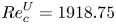 ${{Re}}^U_c= 1918.75$ (last line in table 1). Since the critical Reynolds numbers obtained agree very well with the results from the literature, in particular with those of Kuhlmann & Albensoeder (Reference Kuhlmann and Albensoeder2014) and Gelfgat (Reference Gelfgat2019), both the steady solver and the eigenvalue solver are considered verified. The corner singularities were not treated in any particular way, because the regularity of the numerical solution was almost unaffected.
Table 2. Eigenvalues  $\sigma _1 +\textrm {i} \omega _1$ for Reynolds numbers
  $ { {Re}}^U_c$ close to the critical point.

4. Results
At low Reynolds number the basic flow in the shear-driven cube  $\boldsymbol {q}_0 = (\boldsymbol {u}_0,p_0)^{\mathrm {T}}$ is steady with time translation symmetry
  $\boldsymbol {q}_0(\boldsymbol {x},t) = \boldsymbol {q}_0(\boldsymbol {x},t+t')$, where
  $t'$ is arbitrary. The basic flow is also invariant under the spatial mirror symmetry map
  $\mathcal {M}$:
 \begin{equation} \mathcal{M}: (u_0, v_0,w_0)(x,y,z) \rightarrow (u_0, v_0,-w_0,)(x,y,-z). \end{equation}
For any mirror symmetric flow the velocity component  $w=0$ vanishes in the midplane
  $z=0$.
The basic flow can lose its stability by the breaking of either the translational invariance in  $t$, the spatial symmetry (4.1) or both. From the linear stability equations, perturbations
  $\tilde {\boldsymbol {q}}$ of the symmetric basic state
  $\boldsymbol {q}_0$ must either be mirror-symmetric, satisfying the same spatial symmetry
  $\mathcal {M}$ as the basic flow, or antisymmetric, satisfying
 \begin{equation} (\hat{u},\hat{v},\hat{w})(x,y,z) =(-\hat{u},-\hat{v}, \hat{w})(x,y,-z). \end{equation}
We further define the symmetric velocity field  $\boldsymbol {u}_S$ and the antisymmetric velocity field
  $\boldsymbol {u}_A$ as
 \begin{equation} \left.\begin{gathered} \boldsymbol{u}_S = \tfrac{1}{2}[\boldsymbol{u} + \mathcal{M}(\boldsymbol{u})],\\ \boldsymbol{u}_A = \tfrac{1}{2}[\boldsymbol{u} - \mathcal{M}(\boldsymbol{u})], \end{gathered}\right\} \end{equation}
with  $\boldsymbol {u} = \boldsymbol {u}_S + \boldsymbol {u}_A$. The kinetic energies
  $E_S$ and
  $E_A$ associated with the symmetric and antisymmetric part of the flow are
 \begin{equation} \left.\begin{gathered} E_S = \tfrac{1}{2}\int_V |\boldsymbol{u}_S|^2 \,\textrm{d} V = \tfrac{1}{8}\int_V |\boldsymbol{u} + \mathcal{M}(\boldsymbol{u})|^2\, \textrm{d} V,\\ E_A = \tfrac{1}{2}\int_V |\boldsymbol{u}_A|^2 \,\textrm{d} V = \tfrac{1}{8}\int_V |\boldsymbol{u} - \mathcal{M}(\boldsymbol{u})|^2\, \textrm{d} V. \end{gathered}\right\} \end{equation}
We note that the total energy of the flow is
 \begin{align} E = \tfrac{1}{2} \int_V |\boldsymbol{u}|^2 \,\textrm{d} V = \tfrac{1}{2} \int_V |\boldsymbol{u}_S + \boldsymbol{u}_A|^2\, \textrm{d} V \leqslant \tfrac{1}{2} \int_V |\boldsymbol{u}_S|^2 \textrm{d} V + \tfrac{1}{2} \int_V |\boldsymbol{u}_A|^2 \,\textrm{d} V = E_S + E_A. \end{align}
To quantify the symmetry or asymmetry of a flow state, one defines the symmetry and asymmetry parameters, respectively, as
 $$\begin{gather} {\mathcal{S}} = \frac{E_S}{E} = \frac{1}{8E}\int_V |\boldsymbol{u} + \mathcal{M}(\boldsymbol{u})|^2 \,\textrm{d} V, \end{gather}$$
 $$\begin{gather}{\mathcal{A}} = \frac{E_A}{E} = \frac{1}{8E}\int_V |\boldsymbol{u} - \mathcal{M}(\boldsymbol{u})|^2 \,\textrm{d} V. \end{gather}$$
 As the Reynolds number is increased a sequence of instabilities can be identified. The qualitative structure of the bifurcations and the naming convention for the different bifurcation points and solutions are sketched in figure 4. The basic mirror-symmetric steady state  $S$, the low Reynolds number part of which up to point
  $F_1$ is denoted
  ${S}_1$, is linearly stable until a pitchfork bifurcation
  ${P}$, where it becomes unstable to a non-oscillating antisymmetric mode
  $\hat {\boldsymbol {q}}_{P}$. This critical mode saturates in the asymmetric steady state
  ${A}$ or its antisymmetric counterpart
  $A'$. Upon increase of the Reynolds number, the now unstable basic flow
  ${S}_1$ loses its stability with respect to an antisymmetric oscillating mode
  $\hat {\boldsymbol {q}}_{{H}_S}$ at the Hopf bifurcation point
  ${H}_S$. For slightly larger Reynolds number the solution
  $S$ develops a fold. The unstable symmetric solution between the saddle node points
  $F_1$ and
  $F_2$ is denoted
  $S_2$, while the solution past
  $F_2$ is denoted
  $S_3$. The large Reynolds number solution
  $S_3$ remains unstable to antisymmetric perturbations, but stable to symmetric perturbations.

Figure 4. Sketch of critical points and bifurcating solutions in the space spanned by the Reynolds number  $ { {Re}}_\tau$ and the square root of the symmetry parameter
  $\sqrt {\mathcal {S}}$ and of that of the antisymmetry parameter
  $\sqrt {\mathcal {A}}$. Linearly stable solutions are indicated by full lines, unstable ones by dashed lines. The blue solution branches are confined to the plane
  $\sqrt {\mathcal {A}}=0$ (bright blue). The two red branches emerging from
  ${P}$ are located above and below the plane
  $\sqrt {\mathcal {A}}=0$.
The asymmetric steady state  ${A}$ (respectively,
  ${A}'$) is stable until a Hopf bifurcation
  ${H}_{1}$ (respectively,
  ${H}_{1}'$), where it becomes unstable to an oscillating mode
  $\hat {\boldsymbol {q}}_{{H}_{1}}$ (respectively,
  $\hat {\boldsymbol {q}}_{{H}_{1}'}$). As the oscillation saturates, the system settles on a limit cycle
  ${{L}_{1}}$ (respectively,
  ${L}_{1}'$). Upon increasing the Reynolds number
  ${A}$ (respectively,
  ${A}'$) becomes unstable to a second oscillating mode
  $\hat {\boldsymbol {q}}_{{H}_{2}}$ in a Hopf bifurcation
  ${H}_{2}$ (respectively,
  ${H}_{2}'$). The limit cycles
  ${{L}_{1}}$ and
  ${L}_{1}'$ destabilise at points
  $I$ and
  $I'$, and a complex dynamics between the two limit cycles arises.
4.1. Stability of the symmetric basic flow
4.1.1. Structure of the symmetric basic flow  $S_{1}$

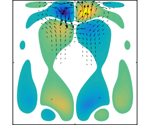
Figure 5 shows the steady symmetric basic flow  $S_{1}$ for
  $ { {Re}}_\tau = 231.19$. This value is slightly less than the critical Reynolds number for the loss of symmetry. The flow structure is similar to the one in the cubic lid-driven cavity (Feldman & Gelfgat Reference Feldman and Gelfgat2010). The flow along the free surface
  $y=0.5$ accelerates as it leaves the upstream edge at
  $(x,y)=(0.5,0.5)$ and reaches (global) maxima with magnitude of
  $\max |\boldsymbol {u}_0|=1851.7$
  $(= { {Re}}_{U_{max}})$ at
  $(x, y, z)=(-0.380, 0.5,\pm 0.449)$. The maxima are located close to the downstream edge
  $(x,y)=(-0.5,0.5)$ of the free surface. The average free-surface velocity is
  $\overline {\boldsymbol {u}_{0,{fs}}} = (-1278.8,0,0)^{\textrm {T}}$ (and
  $ { {Re}}_{U_{avg}}=1278.8$). The main characteristic of the flow is a core vortex aligned with the spanwise direction, best seen in figure 5(a). Similar as in the cubic lid-driven cavity, the swirling motion slows down in the vicinity of the end walls at
  $z=\pm 0.5$ and two mirror symmetric vortical structures arise near the end walls which have the tendency to form ring-like vortices (figure 5b,c) due to the Bödewadt mechanism (Bödewadt Reference Bödewadt1940). Considering the local helicity
  $\boldsymbol {u}\boldsymbol {\cdot }\boldsymbol {\omega }$, where
  $\boldsymbol {\omega }= \boldsymbol {\nabla }\times \boldsymbol {u}$ is the vorticity, we notice that in the plane
  $y=0$ the
  $y$-contribution to the local helicity
  $v\omega _y$ takes its local extrema at the locations indicated by the pink dots. These properties will be used later for comparison.

Figure 5. Basic flow  $S_{1}$ at
  $ { {Re}}_\tau = 231.19 < { {Re}}_{P}$ in the planes
  $z=0$ (a),
  $x=0$ (b) and
  $y=0$ (c). Arrows denote the in-plane components of the velocity vector, while the colour map shows velocity normal to the plane shown. Along the green lines the spanwise velocity
  $w_0=0$ vanishes. Global extrema of
  $v\omega _y$ are indicated by pink dots.
The two ring-like end wall vortices lead to a spanwise velocity directed towards the symmetry plane  $z=0$ within a region near
 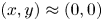 $(x,y)\approx (0,0)$, while the spanwise flow is directed away from the symmetry plane near the walls
  $x=\pm 0.5$ and
  $y=-0.5$. On the free surface at
  $y=0.5$ the flow has a small component directed towards the symmetry plane. These regions are separated by the surfaces characterised by
  $w=0$, the contours of which are shown in figure 5(b,c) by dark green lines.
4.1.2. First bifurcation of $S_{1}$ to the steady asymmetric flow ${A}$


As the Reynolds number is increased, the mirror symmetry is lost. The spectrum of the linear stability operator slightly above the critical Reynolds number, shown in figure 6, reveals the first eigenvalue to cross the imaginary axis has  $\omega =\textrm {Re}(\gamma )=0$. Interpolation of the subcritical and supercritical growth rates near the critical point
  ${P}$ yields a critical Reynolds number of
  $ { {Re}}_{P} = 231.28$. The spanwise velocity
  $w(x,y)\neq 0$ in the midplane
  $z=0$ of the leading and supercritical eigenmode is non-zero (figure 7a). Therefore, this mode breaks the mirror symmetry (4.1). The corresponding critical Reynolds number based on the maximum surface velocity
 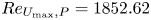 $ { {Re}}_{U_{\max },P}= 1852.62$ compares very well with the critical Reynolds number
 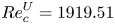 $ { {Re}}^U_c=1919.51$ for the lid-driven cube (Kuhlmann & Albensoeder Reference Kuhlmann and Albensoeder2014), even though the critical mode in the cube is oscillatory and subcritical with the saddle-node point at
  $ { {Re}}^U_c=1906.0$. The critical Reynolds number based on the average velocity
  $ { {Re}}_{U_{avg},P}= 1279.47$ is much lower.

Figure 6. Eigenvalue spectrum of the linear stability problem for the basic flow at the supercritical Reynolds number  $ { {Re}}_\tau = 231.73$. The grey shade indicates the region of negative growth rates
  $\sigma ={\rm Re}(\gamma )<0$.

Figure 7. Spanwise velocity field in the plane  $z=0$ of (a) the slightly supercritical eigenmode
  $\hat w_{P}(x,y)$ for
  $ { {Re}}_\tau =231.73$, and of (b) the velocity field
  $w_{A}(x,y)$ of the slightly supercritical nonlinear steady-state
  ${A}$ obtained by numerical simulation for
  $ { {Re}}_\tau = 232.38$. The dashed lines correspond to (a)
  $\hat {w}_{P}=0$ and (b)
  $w_{A}=0$. The marker
  $(\blacksquare )$ in (b) indicates the monitoring point
  $\boldsymbol {x}_p = (0.4,0,0)^\mathrm {T}$.
The result of the linear stability analysis is confirmed by the full numerical simulation. At  $ { {Re}}_\tau =232.38$ (
 $ { {Re}}_{U_{max}}=1866.4$,
  $ { {Re}}_{U_{avg}}=1288.0$) the deviation of nonlinear steady state
  ${A}$ from the symmetric steady state
  ${S}_1$ exhibits essentially the same structure as the linear mode at
  $ { {Re}}_\tau =231.73$, except from small nonlinear corrections. This is demonstrated in figure 7(b). The isolines of
  $w_{A}(z=0)$ are almost indistinguishable from those of the eigenfunction
  $\hat {w}_{P}$ shown in figure 7(a).
Apart from the solution branch  ${A}$, also a solution branch
  ${A}'$ exists which is distinguished from
  ${A}$ by the asymmetric part of the flow having the opposite sign. The two nonlinear states
  ${A}$ and
  ${A}'$ emerge from the critical point
  ${P}$, and both originate from the same real-valued linear mode but with amplitudes of different sign. To distinguish between
  ${A}$ and
  ${A}'$ we associate with
  ${A}$ the steady state in which
  $w(\boldsymbol {x}_p)>0$, and with
  ${A}'$ its mirror symmetric counterpart with
  $w(\boldsymbol {x}_p)<0$, where the monitoring point
  $\boldsymbol {x}_p = (0.4,0,0)^\mathrm {T}$ has been selected arbitrarily. It is marked by a black square
  $(\blacksquare )$ in figure 7(b).
The global structure of the steady antisymmetric eigenmode  $\hat {\boldsymbol {q}}_{P}$ at
  $ { {Re}}_\tau = 231.73$ (
 $ { {Re}}_{U_{max}}=1857.81$,
  $ { {Re}}_{U_{avg}}=1282.86$) for slightly supercritical conditions is illustrated in figure 8. The breaking of the mirror symmetry is obvious from the isosurfaces of
  $\hat {w}$ shown in figure 8(c). The perturbation velocity field is primarily located near the upstream wall at
  $x=0.5$ and extends upstream of the basic flow. Furthermore, the perturbation velocity exhibits strong components in the streamwise direction, parallel to the basic flow. From the isosurfaces for
  $\hat {u}$ and
  $\hat {v}$ with large positive (yellow) and negative (purple) values the perturbation flow primarily consists of a single slender vortex located in midplane
  $z=0$ and extending over the solid walls. This structure can be clearly seen from figure 8(d) which shows the structure of the vortex in the horizontal plane
  $y=-0.2$ in the lower half of the cavity. The location and shape of the single vortex is very similar to the periodic Taylor–Görtler vortices known from the spanwise extended lid-driven cavity (Koseff et al. Reference Koseff, Street, Gresho, Upson, Humphrey and To1983; Koseff & Street Reference Koseff and Street1984a; Albensoeder et al. Reference Albensoeder, Kuhlmann and Rath2001b; Kuhlmann & Romanò Reference Kuhlmann and Romanò2019). We denote the vortex a single Taylor–Görtler vortex, because it is created by the same instability mechanisms which are also responsible for the Taylor–Görtler vortices in the periodic lid-driven cavity, as further explained below.

Figure 8. Leading stationary eigenmode  $\hat {\boldsymbol {q}}_{P}(\boldsymbol {x})$ at
  $ { {Re}}_\tau =231.73$. Velocity components
  $\hat {u}_P$ (a),
  $\hat {v}_P$ (b) and
  $\hat {w}_P$ (c) of the isosurfaces are shown at
  $\pm 20\,\%$ of their respective extrema (yellow, >0; purple, <0). The arrow indicates the direction of the surface stress. (d) Structure in the plane
  $y=-0.2$. Arrows indicate the cross-stream velocity field
  $(\hat {u}_P,\hat {w}_P)$, while colour indicates the velocity component
  $\hat {v}$.
At the critical Reynolds number  $ { {Re}}_{P}$ the asymmetric steady flows
  ${A}$ and
  ${A}'$ (figure 4) bifurcate supercritically from the symmetric basic state
  ${S}_1$. We find the steady asymmetric mode grows to a finite amplitude which saturates for
  $t\to \infty$. To compute the saturated flow state
  ${A}$ the unsteady solver was run for
  $ { {Re}}_\tau =232.38$ until the time derivative of the total kinetic energy
  $\partial E/\partial t$ became less than
  $10^{-5}$. Thereafter, the flow state
  ${A}$ was computed for successively decreasing Reynolds numbers using the steady solver. As a measure for the amplitude of the deviation from the symmetric flow the asymmetry measure
  $\mathcal {A}$ was evaluated and fitted by
 \begin{equation} {\mathcal{A}}( {{Re}}_\tau) = a_1( {{Re}}_\tau - a_2)^{a_3}. \end{equation}
The result is shown in figure 9 with exponent  $a_3=0.9612\approx 1$. For a generic pitchfork bifurcation, the deviation of the flow from the basic flow scales as the square root of the distance from the critical point. Since the asymmetry measure
  $\mathcal {A}$ (4.6b) is quadratic in the velocity deviation, the linear scaling
  ${\mathcal {A}}( { {Re}}_\tau ) \sim { {Re}}_\tau - { {Re}}_{P}$ found signals a pitchfork bifurcation at
  $ { {Re}}_{P} = a_2 = 231.28$ (
 $ { {Re}}_{{P}, max}=1854.71, { {Re}}_{{P}, avg}=1281.32$). This critical Reynolds number, determined by nonlinear simulation, matches perfectly the value obtained by the linear stability analysis.

Figure 9. Asymmetry measure  $\mathcal {A}$ as a function of the distance of the shear stress Reynolds number from the critical point
  $ { {Re}}_{P}$. Open symbols represent numerical simulations. The function
 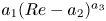 $a_1( { {Re}}-a_2)^{a_3}$ with
  ${a_1=4.513^{-5}}$,
  $a_2=231.29$ and
  $a_3=0.9526$ is represented by a full line.
The saturated asymmetric flows  ${A}$ and
  ${A}'$ do not differ much from the basic flow
  $S_{1}$. The strength of the Taylor–Görtler perturbation vortex centred on the midplane is so weak that it can barely be recognised on the background of the end-walls vortices of
  $S_{1}$. The maximum value of the magnitude of the velocity is
 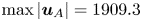 $\max |\boldsymbol {u}_{A}|=1909.3$ at
 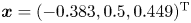 $\boldsymbol {x} = (-0.383, 0.5, 0.449)^{\mathrm {T}}$ and the average flow at the surface is
  $\langle {\boldsymbol {u}_{A}}\rangle _{y=1/2}= (-1316.1, 0, 0.371)^{\mathrm T}$ reflecting the broken symmetry with a net spanwise flow on the top surface. This weak symmetry breaking is also visible by the isolines
  $w_{A}=0$ shown in dark green in figure 10(a,b). In particular, the spanwise velocity on the midplane
  $w_{A}(z=0)$ is non-zero, but distinct cells cannot be recognised.

Figure 10. Saturated asymmetric flow  $\boldsymbol {u}_{A}$ for
  $ { {Re}}_\tau = 236.01$ shown in the planes
  $x=0$ (a) and
  $y=0$ (b). Arrows show the in-plane velocity components. The colour code indicates the velocity component normal to the plane shown. Green lines denote isolines
  $w_{A}=0$. Loci of the global extrema of
  $v_{A} \omega _{y,{A}}$ are indicated by the pink dots.
4.1.3. Second instability of $S_{1}$

Even though the symmetric basic state is unstable for  $ { {Re}}_\tau > { {Re}}_{P}$, further instabilities are of interest, because the bifurcating solutions can significantly affect the dynamics of supercritical chaotic flow (Loiseau et al. Reference Loiseau, Robinet and Leriche2016; Lopez et al. Reference Lopez, Welfert, Wu and Yalim2017). At
  $ { {Re}}_{{H}_S}=232.61$, only approximately
  $0.5$ % above
  $ { {Re}}_{P}$ a pair of complex eigenvalues with
  $\omega _{{H}_S}=689.68$ crosses the imaginary axis. The index
  ${H}_S$ refers to the Hopf bifurcation point
  ${H}_S$ in figure 4. These eigenvalues are shown as a pair of black circles in figure 6 for
  $ { {Re}}_\tau =231.79 < { {Re}}_{{H}_S}$. By
  $ { {Re}}_{{H}_S}=232.61$ the real parts of these eigenvalues have overtaken the second largest purely real eigenvalue.
The oscillating eigenmode  $\hat {\boldsymbol {q}}_{{H}_S}$ is antisymmetric at any instant of time, just like the stationary mode
  $\hat {\boldsymbol {q}}_{P}$. The mode also consists of a single Taylor–Görtler vortex centred on the midplane
  $z=0$. This is demonstrated in figure 11 which shows the temporal evolution of the structure of the mode over one half of the period in the plane
  $y=-0.2$ (the slightly negative growth rate is disregarded in the visualisation in figure 11). Like the stationary mode
  $\hat {\boldsymbol {q}}_{P}$, the mode
  $\hat {\boldsymbol {q}}_{{H}_S}$ mainly extends along the solid wall upstream of the free surface. It can be seen that the Taylor–Görtler vortex periodically changes its sense of rotation. The sense of rotation also varies spatially along the apparent centreline of the Taylor–Görtler vortex. This can be seen from the temporal evolution of the isosurfaces of
  $\hat {u}$,
  $\hat {v}$ and
  $\hat {w}$ over half a period shown in figure 12. From figure 12(c) the spanwise velocity
  $\hat w$ in the midplane
  $z=0$ and near the bottom wall
  $y=-0.5$ (
 $\hat w < 0$, purple) changes its sign downstream of the basic flow near the upstream wall
  $x=0.5$ (
 $\hat w > 0$, yellow).

Figure 11. Temporal evolution of the oscillatory antisymmetric eigenmode  $\hat {\boldsymbol {q}}_{{H}_S}$ at
  $ { {Re}}_{{H}_S} = 232.59$ in the plane
  $y=-0.2$ shown at (a)
  $t=0$, (b)
  $t=T_{{H}_S}/6$ and (c)
  $t=2T_{{H}_S}/6$, where
  $T_{{H}_S}=2{\rm \pi} /\omega _{{H}_S}$. Arrows show the velocity vectors
  $(\hat {u}_{H_{S}},\hat {w}_{H_{S}})$ in the plane while the velocity component
  $\hat {v}_{{H_S}}$ is shown by colour. For the visualisation the (negative) growth rate is disregarded here, as well as in all following figures displaying the time evolution of critical modes.

Figure 12. Evolution of the time-dependent antisymmetric eigenmode  $\hat {\boldsymbol {q}}_{{H}_S}$ at
  $ { {Re}}_\tau = 232.59 < { {Re}}_{{H}_S}$. Shown are isosurfaces of
  $\hat {u}_{H_{S}}$,
  $\hat {v}_{H_{S}}$ and
  $\hat {w}_{H_{S}}$ at three instants of time over half a period, (a,b,c)
  $t=0$, (d,e,f)
  $t=T_{{H}_S}/6$ and (g,h,i)
  $t=2T_{{H}_S}/6$. Each isosurface correspond to
  $\pm 0.2\times \max _{\boldsymbol {x}}|\hat {\boldsymbol {u}}|$. Positive and negative values are coded by colour with yellow for >0, and purple for <0. The arrow indicates the direction of the surface stress and grey shows the plane
  $y=-0.2$ on which the flow is illustrated in figure 11. The first movie of the accompanying material shows the evolution of the perturbation velocity magnitude during one period: (a)
  $\hat {u}_{{H}_S}$; (b)
  $\hat {v}_{{H}_S}$; (c)
  $\hat {w}_{{H}_S}$; (d)
  $\hat {u}_{{H}_S}$; (e)
  $\hat {v}_{{H}_S}$; ( f)
  $\hat {w}_{{H}_S}$; (g)
  $\hat {u}_{{H}_S}$; (h)
  $\hat {v}_{{H}_S}$; (i)
  $\hat {w}_{{H}_S}$.
We did not find any stable limit cycle related to the secondary bifurcation form of the basic symmetric flow. Therefore, we could not determine the character of the bifurcation being subcritical or supercritical. The realisation of a stable bifurcating limit cycle is prevented by the much larger linear growth rate of the stationary antisymmetric mode  ${P}$ near
  $ { {Re}}_{{H}_S}$.
4.1.4. Fold bifurcation of S
To probe the further evolution of the symmetric solution  $S$, the solution of (2.4) is constrained to be mirror-symmetric by (2.5). This allows us to track the unstable basic flow
  $S$ to higher Reynolds numbers. Near
  $ { {Re}}_\tau \approx 232$ solution
  $S$ exhibits a fold which is visualised by
  $E( { {Re}}_\tau )$ in figure 13. The first saddle-node bifurcation point
  ${F}_1$ associated with the fold arises at
  $ { {Re}}_{{F}_1}=232.62$ (
 $ { {Re}}_{{F}_1, max}=1867.89$,
  $ { {Re}}_{{F}_1, avg} = 1289.44$). This value is extremely close to the Hopf bifurcation point at
  $ { {Re}}_{{H}_S}=232.61$ on
  $S_{1}$. Beyond
  $F_1$ the mirror-symmetric solution S turns backward (dashed curve) and is named
  $S_2$. It is unstable with respect to mirror-symmetric perturbations. At the lower Reynolds number
  $ { {Re}}_{{F}_2}=231.60 < { {Re}}_{{F}_1}$ (
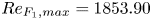 $ { {Re}}_{{F}_1, max}=1853.90$,
  $ { {Re}}_{{F}_1, avg} = 1280.12$) a second saddle-node bifurcation arises and the solution branch S turns forward again, now named
  $S_3$. The flow
  $S_3$ regains stability with respect to mirror-symmetric perturbations, but remains unstable to antisymmetric perturbations.

Figure 13. Kinetic energy  $E=E_S$ as a function of the Reynolds number
  $ { {Re}}_\tau$. Full (open) symbols denote stable (unstable) states in the symmetric subspace. The lines are guides to the eye, connecting the data points. The short vertical dotted line marks the Hopf bifurcation point at
  $ { {Re}}_{{H}_S}$ on
  $S_{1}$. The large open symbols represent points for which the basic flow and the unstable mode shown in figure 14 (open square) and the growth rate of the unstable mode in figure 16 (diamond).
The fold bifurcation is associated with a pair of mirror symmetric Taylor–Görtler vortices which can exist at this Reynolds number. We find that the intermediate state  $S_2$ is unstable to a stationary mode consisting of a pair of counter-rotating Taylor–Görtler vortices which are mirror symmetric. The vortex pair can have two directions of rotation, depending on the sign of the unstable mode and characterised by
  $\hat {u}(\boldsymbol {x}_p) \lessgtr 0$. Figure 14 shows the unstable basic flow
  $S_2$ with
  $u(\boldsymbol {x}_p)< 0$ and the two-vortex Taylor–Görtler mode with
  $\hat {u}(\boldsymbol {x}_p)>0$. As shown in figure 15 the growth rate (corresponding to the second largest real eigenvalue in figure 6) as a function of
  $ { {Re}}_\tau$ exhibits a maximum and vanishes as the saddle node points
  $F_1$ and
  $F_2$ are approached.

Figure 14. (a) Unstable basic state  $S_2$ and (b) growing corotating eigenmode at
  $ { {Re}}_\tau = 232.06$ close to its maximum growth rate (open square in figure 15). Both flows are shown in the plane
  $y=0$. Colour indicates the velocity component normal to the pane displayed. Full square indicates the probing point
  $\boldsymbol {x}_p$.

Figure 15. Growth rate  $\textrm {Re}(\gamma )$ (circles, full squares and full triangles) of symmetric Taylor–Görtler vortices across the fold bifurcation involving section
  $S_{1}$,
  $S_2$ and
  $S_3$ of the symmetric solution
  $S$ (labels, symbol type) shown as a function of
  $ { {Re}}_\tau$. The saddle-node bifurcation points
  $F_1$ and
  $F_2$ are indicated by vertical dashed lines. The open square corresponds to the growth rate of the perturbation flow shown in figure 14(b). The line is an interpolation of the discrete data.
The nonlinear evolution of small symmetric perturbations of  $S_2$ at constant
  $ { {Re}}_\tau$ is such that the amplitude of the unstable Taylor–Görtler mode grows until the flow saturates either in
  $S_1$ or in
  $S_3$. Perturbations in form of Taylor–Görtler vortices with
  $\hat {u}(\boldsymbol {x}_p)>0$ which rotate in the same direction (in the plane
  $y=0$) as the Bödewadt eddies saturate in
  $S_{1}$, while Taylor–Görtler vortices with
  $\hat {u}(\boldsymbol {x}_p)<0$ counter-rotating with respect to the Bödewadt eddies saturate in
  $S_3$. Since the Taylor–Görtler vortices have the same symmetry as the underlying symmetric main overturning flow including the Bödewadt eddies, the Taylor–Görtler vortices cannot be separated from the flow states
  $S_{1}$ and
  $S_3$. From the dynamics of the perturbations of the unstable flow
  $S_2$, however, we can conclude that the flow states
  $S_{1}$ and
  $S_3$ contain finite-amplitude Taylor–Görtler vortex contributions. Since the Taylor–Görtler vortices included in the flow state
  $S_{1}$ are corotating with the Bödewadt eddies, they cannot be visually identified in the projection of the flow field. However, within
  $S_3$ the Taylor–Görtler vortex contribution can be clearly identified in figure 16(b) for
  $ { {Re}}_\tau =232.70$ (
 $ { {Re}}_{U_{max}}=1863.9$,
  $ { {Re}}_{U_{avg}}=1287.8$) by the small vortices counter-rotating with respect to the larger Bödewadt circulation. The extrema of
  $v\omega _y$ in the plane
  $y=0$ (pink dots in figure 16b) are located within these Taylor–Görtler vortices. In figure 16(b) the separated vortices near the midplane approximately occupy the region
  $(x,z) \in [0.4,0.5]\times [-0.1,0.1]$. They are not so clearly visible in figure 16(a) where the vortices are approximately located in
  $(y,z) \in [0.4,0.5]\times [-0.1,0.1]$.

Figure 16. Mirror-symmetric flow  $\boldsymbol {u}_{{S}_3}$ at
  $ { {Re}}_\tau = 232.70$ shown in the plane
  $x=0$ (a) and
  $y=0$ (b). Arrows show the in-plane velocity components. The colour code indicates the velocity component normal to the plane shown. Green lines denote isolines
  $w_{S_3}=0$. Global extrema of
  $v_{S_3}\omega _y, {S_3}$ are indicated by the pink dots.
Depending on the sense of rotation of the Taylor–Görtler contribution to the total symmetric flow they are either suppressed or favoured by the Bödewadt eddies which always have the same sense of rotation. From the dynamics near  $S_2$ we conclude that Taylor–Görtler vortices counter-rotating with respect to the Bödewadt eddies (
 $\hat {u}(\boldsymbol {x}_p)<0$) are favoured in
  $S_3$ (for large
  $ { {Re}}_\tau$), whereas Taylor–Görtler vortices corotating with respect to the Bödewadt eddies (
 $\hat {u}(\boldsymbol {x}_p)>0$) are favoured in
  $S_{1}$ (for small
  $ { {Re}}_\tau$). Since the Taylor–Görtler vortices contained in
  $S_{1}$ and
  $S_3$ have a finite amplitude the competition between
  $S_{1}$ and
  $S_3$ leads to the observed hysteresis creating the fold of
  $S$. It is likely that the fold originated from a cusp point in an extended parameter space in which an additional parameter can tune (reduce) the interaction of the Taylor–Görtler vortices with the Bödewadt flow. One such parameter could be the spanwise aspect ratio (e.g. see Kuhlmann, Wanschura & Rath Reference Kuhlmann, Wanschura and Rath1997; Albensoeder et al. Reference Albensoeder, Kuhlmann and Rath2001b). A computation of the fold as a function of the aspect ratio is, however, computationally expensive and other symmetric Taylor–Görtler modes may come into play.
4.2. Time-dependent asymmetric flow
4.2.1. Linear stability analysis of the steady asymmetric flow ${A}$

To investigate the linear stability of the steady asymmetric flow the solution branch  ${A}$ is tracked using the BoostConv algorithm in combination with the second-order time-integration scheme. The basic state for the stability analysis now refers to
  ${A}$. Since the flow
  ${A}$ has no spatial symmetries, the normal modes will likewise have no spatial symmetries. The stability analysis yields a Hopf bifurcation at
  $ { {Re}}_{{H}_{1}}= 236.04$. The critical frequency
  $\omega _{{H}_{1}} = 764.16$ is only approximately 10 % larger than
  $\omega _{{H}_S}$. Correspondingly, the solution
  ${A}'$ becomes unstable at the same Reynolds number with respect to the Hopf mode
  ${H}_{1}'$ with the same frequency.
Figure 17 shows the components of the velocity field of the leading eigenmode  $\hat {\boldsymbol {q}}_{{H}_{1}}$ at the slightly subcritical Reynolds number
 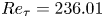 $ { {Re}}_\tau =236.01$. The mode resembles the oscillatory mode
  $\hat {\boldsymbol {q}}_{{H}_S}$ destabilising the symmetric basic state
  $S_{1}$ at
  $ { {Re}}_{{H}_S}$ (figure 12). While mode
  $\hat {\boldsymbol {q}}_{{H}_S}$ is an antisymmetric standing wave, the mode
  $\hat {\boldsymbol {q}}_{{H}_{1}}$ travels in the negative
  $z$ direction. The propagating Taylor–Görtler vortices are oriented slightly oblique which is illustrated in figure 18. Similarly, the mode
  $\hat {\boldsymbol {q}}_{{H}_{1}'}$ which destabilises the asymmetric state
  ${A}'$ travels in the positive
  $z$ direction. The travelling direction is dictated by the particular asymmetric basic flow state
  ${A}$ or
  ${A}'$.

Figure 17. Evolution of the time-dependent asymmetric eigenmode  $\hat {\boldsymbol {u}}_{{H}_{1}}$ at
  $ { {Re}}_\tau =236.01$ in the plane
  ${y=-0.2}$ shown at
  $t=0$ (a),
  $t=T_{{H}_{1}}/6$ (b) and
  $t=2T_{{H}_{1}}/6$ (c). Arrows show the velocity vectors
  $(\hat {u}_{{H}_{1}},\hat {w}_{{H}_{1}})$ in the plane while the velocity component
  $\hat {v}_{{H}_{1}}$ is shown by colour.

Figure 18. Evolution of the time-dependent asymmetric eigenmode  $\hat {\boldsymbol {u}}_{{H}_{1}}$ at
  $ { {Re}}_\tau =236.01$. Shown are isosurfaces of
  $\hat {u}_{{H}_{1}}$,
  $\hat {v}_{{H}_{1}}$ and
  $\hat {w}_{{H}_{1}}$ at three instants of time over half a period,
  $t=0$ (a,b,c),
  $t=T_{{H}_{1}}/6$ (d,e,f) and
  $t=2T_{{H}_{1}}/6$ (g,h,i). Isosurfaces corresponding to
  ${\pm }20\,\%$ of the extrema of the velocity component are shown in colour with yellow for >0, and purple for <0. The arrow indicates the direction of the surface stress and grey indicates the plane
  $y=-0.2$ on which the flow is illustrated in figure 17. The second movie of the accompanying material shows the evolution of the perturbation velocity magnitude during one period: (a)
  $\hat {u}_{{H}_{1}}$; (b)
  $\hat {v}_{{H}_{1}}$; (c)
  $\hat {w}_{{H}_{1}}$; (d)
  $\hat {u}_{{H}_{1}}$; (e)
  $\hat {v}_{{H}_{1}}$; ( f)
  $\hat {w}_{{H}_{1}}$; (g)
  $\hat {u}_{{H}_{1}}$; (h)
  $\hat {v}_{{H}_{1}}$; (i)
  $\hat {w}_{{H}_{1}}$.
As for the critical modes of the symmetric basic state  ${S}_1$, the critical modes of the asymmetric steady flows
  ${A}$ and
  ${A}'$ arise in form of one or two (at times) Taylor–Görtler vortices, located in the vicinity of the midplane
  $z=0$ of the cavity. The relatively small deviation of the steady asymmetric flows states
  ${A}$ and
  ${A}'$ from the symmetric basic state
  $S_{1}$ (compare figure 5b,c with figure 10a,b) suggests that the onset of asymmetric oscillations is not caused by the asymmetry of the steady basic flow, but is rather an instability similar to the one of the symmetric steady flow
  $S_{1}$ which is destabilised by critical mode
  $\hat {\boldsymbol {q}}_{{H}_S}$ and its complex conjugate mode
  $\hat {\boldsymbol {q}}_{{H}_S'}$. The asymmetric part of the three-dimensional steady flow seems to merely make the modes propagate and suppress the onset of oscillations for a small range of Reynolds numbers
  $ { {Re}}_\tau \in [ { {Re}}_{{H}_S}, { {Re}}_{{H}_{1}}]$. This interpretation is confirmed by the mean energy budget later.
4.2.2. Finite amplitude oscillations of the asymmetric flow
For  $ { {Re}}_\tau > { {Re}}_{{H}_{1}}$ the amplitude of oscillation of the asymmetric flow saturates and reaches the limit cycle
  ${{L}_{1}}$. To investigate the saturation, the third-order time-integration scheme BDF3/EXT3 has been used. Let us introduce the peak-to-peak amplitude
  $\Delta \mathcal {A}$ of the asymmetry measure
  $\mathcal {A}$ of the fully developed nonlinear periodic flow with constant oscillation amplitude. To determine subcritical or supercritical character of the bifurcation the ansatz (4.7) is fitted to
  $\Delta {\mathcal {A}}( { {Re}}_\tau )^2$ using least squares. From the fit shown in figure 19(a) we find the critical Reynolds number
  $ { {Re}}_{{H}_{1}}=a_2= 236.03$ and the exponent
  $a_3=1.0283\approx 1$. Therefore,
  $\Delta \mathcal {A}$ scales almost as the square root of the distance from the critical point and the bifurcation is supercritical. The above estimate of
  $ { {Re}}_{{H}_{1}}$ almost perfectly agrees with the result from the linear stability analysis
  $ { {Re}}_{{H}_{1}}^{lin}= 236.05$. Interpolation of
  $ { {Re}}_{U,{max}}$ and
  $ { {Re}}_{U,{avg}}$ give
  $ { {Re}}_{{H}_1, max}=1909.83$ and
  $ { {Re}}_{{H}_1, avg}=1316.42$, respectively.

Figure 19. (a) Peak-to-peak amplitude  $\Delta {\mathcal {A}}$ of the saturated oscillatory asymmetric flow
  $\boldsymbol {u}_{{L}_{1}}$. The straight line is a fit according to (4.7). (b) Evolution of the spectral amplitudes
  $A$ of the saturated asymmetric nonlinear oscillations flow
  $w_{{L}_{1}}$ at the monitoring point
  $\boldsymbol {x}_p$.
As the Reynolds number increases, higher temporal harmonics are generated. The amplitudes of  $w_{{H}_{1}}(\boldsymbol {x}_p)$ are displayed in figure 19(b). At
  $ { {Re}}_\tau =239.37$, the second and third harmonics have already grown to an appreciable amplitude of
  $0.65 A_1$, and
  $0.18 A_1$, where
  $A_1$ is the amplitude of the fundamental harmonic. The fundamental frequency
  $\omega _{{{L}_{1}}}=764.5$ does not vary much in range of Reynolds numbers considered and agrees well with the frequency obtained by the linear stability analysis
  $\omega _{{{L}_{1}}}^{lin}= 764.16$. Due to the two asymmetric steady solutions
  ${A}$ and
  ${A}'$ there also exists a corresponding limit cycle
  ${L}_{1}'$ near
  ${A}'$.
The bifurcation diagram from  $S_{1}$ to
  ${A}$ and to
  ${H}_{1}$ in terms of the asymmetry measure
  $\mathcal {A}$ is shown in figure 20. The bifurcations to
  ${A}'$ and
  ${H}_{1}'$ are included by plotting
  $\mathrm {sign}[w(\boldsymbol {x}_p)]\times \mathcal {A}^{1/2}$. Lines are guides to the eye and line intersections do not accurately reflect the critical Reynolds numbers.

Figure 20. Bifurcation of solutions as function of the asymmetry parameter  $\mathcal {A}$. Symbols show the results of the numerical simulations, lines have been drawn as guides to the eye, where stable (unstable) branches are shown by full (dashed) lines. The grey shading indicates the range of peak-to-peak oscillation of
  $\mathcal {A}$ of the limit cycles
  ${L}_{1}$ and
  ${L}_{1}'$.
4.2.3. Further destabilisation of the steady asymmetric flow
As one continues increasing the Reynolds number, the asymmetric solution branch  ${A}$ is destabilised at
  $ { {Re}}_{{H}_{2}}\approx 237.07$ (
 $ { {Re}}_{{H}_2, max}=1921.78$,
  $ { {Re}}_{{H}_2, avg}=1324.33$) by a second oscillatory mode. The associated frequency is
  $\omega _{{H}_{2}} = 82.55$. It is approximatively 10 times smaller than the frequency
  $\omega _{{H}_{1}}$ of the limit cycle
  ${{L}_{1}}$. Again, the energy budget of the neutral mode
  $\hat {\boldsymbol {q}}_{{H}_{2}}$ is extremely similar to the ones of all previous modes, indicating the steady state
  ${A}$ is destabilised by the same centrifugal mechanism. The mode
  $\hat {\boldsymbol {q}}_{{H}_{2}}$ (respectively,
  $\hat {\boldsymbol {q}}_{{H}_{2}'}$) consists of three vortices which are travelling in the negative (respectively, positive)
  $z$ direction. Figures 21 and 22 illustrate the structure of the neutral mode
  $\hat {\boldsymbol {q}}_{{H}_{2}}$ with Taylor–Görtler vortices travelling in the negative
  $z$ direction. Qualitatively, the vortices of mode
  $\hat {\boldsymbol {q}}_{{H}_{2}}$ are more aligned with the streamwise direction of the basic flow than those of mode
  $\hat {\boldsymbol {q}}_{{H}_{1}}$, which tend to be in a slightly more oblique. This is particularly visible for the
  $x$-component of the perturbation velocity (compare figure 18a,d,g with 21a,d,g).

Figure 21. Temporal evolution of the asymmetric eigenmode  $\hat {\boldsymbol {u}}_{{H}_{2}}$ at
  $ { {Re}}_\tau =237.07$. Shown are isosurfaces of
  $\hat {u}_{{H}_{2}}$,
  $\hat {v}_{{H}_{2}}$ and
  $\hat {w}_{{H}_{2}}$ at three instants of time over half a period,
  $t=0$ (a,b,c),
  $t=T_{{H}_{2}}/6$ (d,e,f) and
  $t=2T_{{H}_{2}}/6$ (g,h,i). Yellow (positive) and purple (negative) isosurfaces correspond to
  ${\pm }20\,\%$ of the extrema of the velocity component. The arrow indicates the direction of the surface stress and grey indicates the plane
  $y=-0.2$ on which the flow is illustrated in figure 17. The third movie of the supplementary material shows the evolution of the perturbation velocity magnitude during one period: (a)
  $\hat {u}_{{H}_{2}}$; (b)
  $\hat {v}_{{H}_{2}}$; (c)
  $\hat {w}_{{H}_{2}}$; (d)
  $\hat {u}_{{H}_{2}}$; (e)
  $\hat {v}_{{H}_{2}}$; ( f)
  $\hat {w}_{{H}_{2}}$; (g)
  $\hat {u}_{{H}_{2}}$; (h)
  $\hat {v}_{{H}_{2}}$; (i)
  $\hat {w}_{{H}_{2}}$.

Figure 22. Evolution of the second most unstable mode  $\hat {\boldsymbol {u}}_{{H}_{2}}$ at
  $ { {Re}}_\tau =237.07$ on the asymmetric solution branch
  ${A}$ in the plane
  $y=-0.2$, shown at
  $t=0$ (a),
  $t=T_{{H}_{2}}/6$ (b) and
  $t=2T_{{H}_{2}}/6$ (c) corresponding to figure 21. Arrows show the velocity vectors
  $(\hat {u}_{{H}_{2}},\hat {w}_{{H}_{2}})$ in the plane, while the velocity component
  $\hat {v}_{{H}_{2}}$ is represented by colour.
4.2.4. Instability mechanism
To better understand the instabilities mechanisms at play, we introduce the local rates of change of perturbation kinetic energy
 \begin{equation} \left. \begin{gathered} i_1 = D^{{-}1}\tilde{\boldsymbol{u}}_\perp \boldsymbol{\cdot} \left( \tilde{\boldsymbol{u}}_\perp \boldsymbol{\cdot}\boldsymbol{\nabla}\right) \boldsymbol{u}_0, \quad i_2 = D^{{-}1}\tilde{\boldsymbol{u}}_\parallel \boldsymbol{\cdot} \left( \tilde{\boldsymbol{u}}_\perp \boldsymbol{\cdot} \boldsymbol{\nabla}\right) \boldsymbol{u}_0, \\ i_3 = D^{{-}1}\tilde{\boldsymbol{u}}_\perp \boldsymbol{\cdot} \left(\tilde{\boldsymbol{u}}_\parallel \boldsymbol{\cdot} \boldsymbol{\nabla}\right) \boldsymbol{u}_0, \quad i_4 = D^{{-}1}\tilde{\boldsymbol{u}}_\parallel \boldsymbol{\cdot} \left( \tilde{\boldsymbol{u}}_\parallel \boldsymbol{\cdot} \boldsymbol{\nabla}\right) \boldsymbol{u}_0, \end{gathered}\right\} \end{equation}
where  $D$ is the mean dissipation rate,
 \begin{equation} D = \frac{1}{T}\int_0^T \int_V \boldsymbol{\nabla}\tilde{\boldsymbol{u}} : \boldsymbol{\nabla}\tilde{\boldsymbol{u}}\,\textrm{d} V \,\textrm{d} t \end{equation}
 $\boldsymbol {u}_0$ can be any basic state and
  $\widetilde {\boldsymbol {u}}$ a perturbation of this basic state which has been decomposed into the directions parallel and perpendicular to the local basic flow with
 \begin{equation} \tilde{\boldsymbol{u}}_\| = \frac{(\tilde{\boldsymbol{u}} \boldsymbol{\cdot} \boldsymbol{u}_0) \boldsymbol{u}_0}{\boldsymbol{u}_0 \boldsymbol{\cdot} \boldsymbol{u}_0}, \quad \tilde{\boldsymbol{u}}_\perp{=} \tilde{\boldsymbol{u}} - \tilde{\boldsymbol{u}}_\|. \end{equation}
 The total local energy production is  $i=\sum _{n=1}^4 i_n$. The global rates of change of kinetic energy due to the above four local contributions is obtained by integrating over the volume and averaging over one period
  $T$ of oscillation (in case of a Hopf bifurcation). This leads to the global change rates
 \begin{equation} \left.\begin{gathered} I_1 = \frac{1}{T} \int_{0}^{T}\int_{V} i_1(\boldsymbol{x}, t) \,\textrm{d} V \,\textrm{d} t, \quad I_2 = \frac{1}{T} \int_{0}^{T}\int_{V} i_2(\boldsymbol{x}, t) \,\textrm{d} V\,\textrm{d} t, \\ I_3 = \frac{1}{T} \int_{0}^{T}\int_{V} i_3(\boldsymbol{x}, t) \,\textrm{d} V\,\textrm{d} t, \quad I_4 = \frac{1}{T} \int_{0}^{T}\int_{V} i_4(\boldsymbol{x}, t) \,\textrm{d} V\,\textrm{d} t. \end{gathered}\right\} \end{equation}
Again, these four contributions add to the total global rate of change of kinetic perturbation energy.
The global normalised energy budgets of several linear modes near their points of neutral stability are displayed in table 3. It can be seen that the magnitudes of  $I_n$ for the three modes
  ${P}$,
  ${H}_S$ and
  ${F}_1$ discussed so far are almost the same. Therefore, these modes are then destabilised by the same physical processes which are represented by the different production terms. The similarity of the energy production rates is due to the similarity of the basic flows and the perturbation modes. Since the contribution
  $I_2$ dominates, all these modes are destabilised primarily through to the lift-up mechanism by which the streamwise perturbation flow
  $u_{\|}$ is amplified by transport of basic state momentum in the cross-stream direction due to
  $u_{\perp }$. In a similar context of the lid-driven cavity this lift-up mechanism has been linked to a centrifugal mechanism by Albensoeder et al. (Reference Albensoeder, Kuhlmann and Rath2001b). Briefly, a centrifugal instability results from the exchange of high-angular-momentum fluid at small streamline radii with low-angular-momentum fluid at larger radii (Rayleigh Reference Rayleigh1920; Bayly Reference Bayly1988).
Table 3. Global energy production rates  $I_n$,
  $n=1\dots 4$, due to different physical processes at Reynolds numbers
  $ { {Re}}_\tau$ close to several critical points as indicated. In addition, the eigenvalue
  $\gamma$ whose real part crosses zero at the critical point, and velocity based Reynolds numbers are specified.

The angular momentum exchange process involves a transport of momentum perpendicular to the basic-state streamlines, represented as  $\boldsymbol {u}_\perp \boldsymbol {\cdot } \boldsymbol {\nabla } \boldsymbol {u}_0$. Therefore, the cross-streamline transport
  $\boldsymbol {u}_\perp \boldsymbol {\cdot } \boldsymbol {\nabla } \boldsymbol {u}_0$ of streamwise momentum
  $\boldsymbol {u}_\|$ quantified by
  $i_2$ in the presence of significant streamlines curvature represents a centrifugal exchange process. If this process dominates, as in the present case, the instability may be called centrifugal.
Furthermore, the spatial distributions of the corresponding energy production densities, shown in figure 23, as well as the vortical structures of the perturbation flow are very similar as those for periodic Taylor–Görtler vortices in an extended lid-driven square cavity (figures 11 to 13 in Albensoeder et al. (Reference Albensoeder, Kuhlmann and Rath2001b)) which corroborates the interpretation of the three modes as stationary and time-dependent Taylor–Görtler vortices. Similarly as in Albensoeder et al. (Reference Albensoeder, Kuhlmann and Rath2001b), the local production rate of perturbation kinetic energy takes its maxima around the main vortex figure 23(a) for the antisymmetric mode  $P$, and between two vortices for the symmetric mode
  $F$ figure 23(b). The local rate perturbation production for modes destabilising through Hopf bifurcations are shown in the additional material online.

Figure 23. Isocontours of the energy production densities  $i=i_1+i_2+i_3+i_4$ in the vicinity of the pitchfork bifurcation and the fold bifurcations at the Reynolds numbers indicated in table 3, at isovalue
  $0.5 \max i$. Movies of the isosurfaces of the energy production density
  $i$ near the Hopf bifurcation points
  $H_S$,
  $H_1$ and
  $H_2$ are available in the supplemental online material available at https://doi.org/10.1017/jfm.2023.946. Here (a)
  $i(\hat {\boldsymbol {q}}_P)$ and (b)
  $i(\hat {\boldsymbol {q}}_{F_1})$.
The first modes bifurcating from  ${S}$ at
  $P$ very much resembles the leading eigenmode in the cubic lid-driven cavity problem which arises at
  $ { {Re}}^U_c=1919.51$. (Kuhlmann & Albensoeder Reference Kuhlmann and Albensoeder2014), in particular, the banana-like shapes of the isosurfaces of the velocity perturbation (see, e.g. figure 11 in Feldman & Gelfgat (Reference Feldman and Gelfgat2010) or figure 7 in Kuhlmann & Albensoeder (Reference Kuhlmann and Albensoeder2014) and the associated movie). Yet, in the lid-driven cavity, the critical mode arises in form of time-periodic counter-rotating vortices, while at P the critical mode consists of a single stationary vortex only. The unstable mode in the lid-driven case does, however, graphically resemble the mode becoming unstable at
  ${H_{S}}$, although its eigenfrequency is nearly twice as large (
 $\omega _{c,{U}} \approx 1125$,
  $\omega _{H_S} \approx 690)$. Moreover, for
  $ { {Re}}_{{H_S}} = 232.61$ on
  $S_{1}$ both values
  $ { {Re}}_{U_{max}, H_S} = 1867.72$ and
  $ { {Re}}_{U_{avg},H_S} = 1289.44$ are lower than
  $ { {Re}}^U_c=1919.51$ by
  $3\,\%$ and
  $33\,\%$, respectively.
While  $ { {Re}}_{U_{max}, H_S}$ of the shear-driven cavity compares well with
  $ { {Re}}^U_c$ of the lid-driven cavity, one might have expected that
  $ { {Re}}_{U_{avg},H_S}$ should compare better with
  $ { {Re}}^U_c$. The fact that
  $ { {Re}}_{U_{avg},H_S}$ is 33 % less than
  $ { {Re}}^U_c$ seems to be related to the different boundary conditions for the perturbation flow
  $\boldsymbol {u}'$ in both systems: In the shear-driven cavity the perturbation flow can slip freely in the
  $y$ and
  $z$ direction on
  $y=0.5$ (homogeneous Neumann conditions:
  $\partial u' / \partial y = \partial w' / \partial y = 0$), whereas the perturbation flow in the lid-driven cavity must satisfy no-slip conditions on the lid
  $(\boldsymbol {u}'=0)$. As a result the perturbation flow in the shear-driven cavity will experience less dissipation, quantified by
  $\boldsymbol {\nabla } \boldsymbol {u}' : \boldsymbol {\nabla } \boldsymbol {u}'$, near the moving boundary than the perturbation flow in the lid-driven cavity. Nevertheless, the perturbation flow in the shear-driven cavity can still extract kinetic energy from the velocity gradients of the basic flow in the
  $x$- and
  $z$-directions,
  $\partial u_0/\partial y$ and
  $\partial w_0/\partial y$, near the moving boundary. These arguments may explain the significantly lower value of
  $ { {Re}}_{U_{avg},H_S}$ as compared with
  $ { {Re}}^U_c$. This difference thus does not contradict the analogy between both systems.
4.3. Destabilisation of the limit cycle ${L}_{1}$

For even higher Reynolds numbers the limit cycles  ${L}_1$ and
  ${L}_{1}'$ become unstable within
  $ { {Re}}_\tau \in [238.75, 240.83]$. Long durations of almost periodic oscillations with constant amplitude are interrupted by nonlinear bursts in an intermittent fashion leading to a complex dynamics. Even though the onset Reynolds numbers of these bursts cannot accurately be pinpointed, this is marked as
  ${I}$ in figure 4.
The dynamics is illustrated by the evolution of  $w(\boldsymbol {x}_p,t)$ shown in figure 24(b). If the oscillations near
  ${L}_{1}$ are followed by a burst, the dynamical system may return either to the same limit cycle (
 ${L}_{1}$) or to the limit cycle
  ${L}_{1}'$ which is the asymmetric counterpart of
  ${L}_{1}$. From figure 24(b) one can recognise the switch from the limit cycle
  ${L}_{1}$ to
  ${L}_{1}'$ during a burst event at approximately
  $t=8.5$. The two limit cycles
  ${L}_{1}$ and
  ${L}_{1}'$ can also be distinguished by the mean value
  $\bar {w}(\boldsymbol {x}_p,t)$ (white dashed lines in figure 24) during the phases of regular oscillations. These mean values have a different sign, depending on the limit cycle. The durations of the bursts as well as the time spans of regular oscillations vary.

Figure 24. Time evolution of (a)  $\mathcal {A}(t)$ and of (b)
  $w(\boldsymbol {x}_p,t)$ at
  $ { {Re}}_\tau =239.37$. The mean values of
  $w(\boldsymbol {x}_p,t)$ corresponding to
  ${{L}_{1}}$ and
  ${L}_{1}'$ are indicated by white horizontal dashed lines. (c) Short-time Fourier transform of
  $w(\boldsymbol {x}_p,t)$ with a sliding time window of width
  $\Delta t = 0.6$, roughly corresponding to 75 periods of oscillation. The grey level indicates the spectral amplitude of the signal; only amplitudes larger than
  $10^{-4}$ are displayed.
When the system is locked on one of the limit cycles its spectrum contains only harmonics of the fundamental frequency (figure 24c). During a burst event, however, the power density spreads over a broader bandwidth. The spectrum is broadened in the form of peaks which are almost regularly spaced around the harmonics of the limit cycle. The velocity field in the midplane  $y=0$ is shown in the supplementary movie 7 for both the limit cycle and a burst event.
The bursting events can be subdivided in three distinct phases. In the first phase, the oscillation frequency of the limit cycle decreases, and a continuous band frequency below the harmonic frequencies starts invading the spectrum. Along with it the peak-to-peak amplitude of  $w(\boldsymbol {x}_p)$ shrinks. In the second phase, the flow undergoes strong oscillations. The beat frequency is approximately
  $\omega _{{beat},1}=50\pm 5$. Due to the strong nonlinear interactions, the beating is strongly anharmonic which results in multiple peaks at frequencies
  $\omega = n \omega _{{L}_{1}} \pm m\omega _{beat,1}$ in the short-time spectrum in figure 24(c). During this second phase, the symmetry of the flow varies significantly. For instance
  $\mathcal {A}$ varies from
  $10^{-6}$ to
  $10^{-2}$ in the last burst of figure 24. This indicates that the flow repeatedly returns to a mirror symmetric flow with
  $w(\boldsymbol {x}_p)\approx 0$. In the last phase, the beat frequency of the signal during the return to regular oscillations is
  $\omega _{beat,2}\approx 75\pm 5$ which is close to the frequency
  $\omega _{{H}_{2}}\approx 82$ of the unstable low-frequency limit cycle which is created by the secondary bifurcation
  ${H}_{2}$ from the unstable asymmetric steady solution
  ${A}$. This scenario suggests the limit cycles
  ${{L}_{1}}$ and
  ${L}_{1}'$ have turned into saddle limit cycles which are repelling in at least one phase space direction.
To probe the existence of another unstable limit cycle with a frequency comparable to the beat frequencies found, one may take advantage of the frequency of  ${{L}_{1}}$ being 10 times higher than the hypothesised limit cycle at this Reynolds number. This allows us to design a low pass filter in order to obtain only the dynamics associated with the slowly evolving mode. To that end selective frequency damping (SFD) is used, not to seek the basic flow as usual (Åkervik et al. Reference Åkervik, Brandt, Henningson, Hopffner, Marxen and Schlatter2006), but to eventually find the low-frequency limit cycle. Following the notation of Åkervik et al. (Reference Åkervik, Brandt, Henningson, Hopffner, Marxen and Schlatter2006) the parameters
  $\chi =3000$ and
  ${\varDelta =0.0007}$ are selected, corresponding to a cut-off frequency
  $\omega _c=227$ which is less than one half of
  $\omega _{{H}_{1}}$ (comparable to the frequency of the limit cycle
  ${{L}_{1}}$), but still large enough not to damp oscillations with frequencies
  $\omega \approx 50$ and its second harmonic. Due to a relatively long period of the hypothetical limit cycle this approach is computationally much more economical than other methods to find unstable manifolds, e.g. the tracking of edge states (Itano & Toh Reference Itano and Toh2001; Schneider et al. Reference Schneider, Gibson, Lagha, Lillo and Eckhardt2008; Lopez et al. Reference Lopez, Welfert, Wu and Yalim2017). While the results of a SFD can help understanding the behaviour of the dynamical system, the filtered flow variables do not satisfy the Navier–Stokes equations, but only the filtered Navier–Stokes equations.
Initiating the filtered flow with  $\boldsymbol {q} = \boldsymbol {q}_{A} + \epsilon \hat {{\boldsymbol {q}}}_{{H}_{2}}$, where
  $\boldsymbol {q}_{A}$ is the steady asymmetric flow and
  $\hat {\boldsymbol {q}}_{{H}_{2}}$ the eigenmode
  ${H}_{2}$ which is multiplied by a small constant
  $\epsilon$, the flow initially oscillates with a low frequency of
  $\omega \approx 30$ and exhibits a growing amplitude (figure 25a). At approximately
  $t=1.2$ higher-frequency oscillations of low amplitude develop on the low-frequency signal until the signal
  $w(\boldsymbol {x}_p,t)$ settles, for
  $t>1.8$, on a periodic flow with fundamental frequency
  $\omega \approx 10$ and higher harmonics. These frequencies do not match the beat frequencies or any of the original flow frequencies. Apparently, the low pass filter has further slowed down the existing slow dynamics, an effect which may depend on the strength of the damping parameter
  $\chi$.

Figure 25. Temporal evolution of  $\mathcal {A}$ and
  $w(\boldsymbol {x}_p,t)$ at
  $ { {Re}}_\tau =239.37$ (a) with and (b) without application of the low-pass filter. Panels (ai), (bi) and (aii), (bii) with a grey background show zooms into the signals as indicated by the grey shading in (aiii), (biii). The red dots in panels (ai) and (aii) indicate the instants of times for which the total flow is shown in figure 26.
From figure 25 one can see, however, that the dynamics is similar, except from the different underlying frequencies. In both the filtered and the unfiltered cases, the system passes by an almost symmetric flow state with  $\mathcal {A}\in [10^{-5}, 10^{-4}]$ after which the asymmetry measure
  $\mathcal {A}$ increases in an exponential fashion before oscillations with a frequency close to
  $\omega _{{{L}_{1}}}$ appear. Eventually the oscillations are damped before the system settles again on a nearly symmetric state. It is also seen from figure 25(aii,bii) that the direction in which the symmetry is breaking alternates. To understand the flow states during these periodic patterns, the low-pass filtered velocity field is shown in figure 26 for the instants of time marked by red dots in figure 25(ai,ii,bi,ii). From figure 26(a,b) corresponding to
  $t=3.427$ the flow is nearly symmetric and resembles the basic flow
  ${S}_1$ (compare with figure 5b,c). In particular, the extrema of
  $v\omega _y$ (pink dots) are located near the end walls as for the basic state
  $S_{1}$. At
  $t=3.567$ (figure 26c,d) two nearly symmetric Taylor–Görtler vortices have grown close to the plane
  $z=0$ and within
  $x\in [0.4,0.5]$ near the upstream wall. These vortices are very similar as in the symmetric flow state
  $S_3$ which bifurcates from
  $F_2$ (compare with figure 16a,b). Similarly, the extrema of
  $v\omega _y$ are now located inside of the Taylor–Görtler vortices. In the meantime, symmetry-breaking modes are growing exponentially and the two centred Taylor–Görtler vortices are transported spanwise in the negative
  $z$ direction, as shown in figure 26(e, f). This shift is also signalled by the asymmetric displacement of the extrema of
  $v\omega _y$. In the following evolution of the filtered flow, five Taylor–Görtler vortices are created (not shown) which decay again such that the flow returns to a nearly symmetric state which completes a half-cycle. In the following half-cycle the Taylor–Görtler vortices are displaced in the positive
  $z$ direction. To further quantify the distance in the phase space of the filtered flow from the flow
  ${S}_3$, we show the ratio of kinetic energies
  $E(\boldsymbol {u} - \boldsymbol {u}_{{S}_3}) / E(\boldsymbol {u}_{{S}_3})$ in figure 27. The second red dot is close the local minimum of the ratio of kinetic energies, indicating the instant of closest approach of the filtered flow field to the symmetric flow state
  ${S}_3$. The symmetric flow state
  $S_{1}$ no longer exists at
  $ { {Re}}=239.37$.

Figure 26. Snapshots of the filtered velocity field for  $ { {Re}}_\tau =239.37$ at the times indicated by the red dots in figure 25(a):
  $t=3.427$ (a,b); at
  $t=3.567$ (c,d); and at
  $t=3.607$ (e, f). Thew flow is shown in the
  $x=0$ plane (a,c,e) and in the
  $y=0$ plane (b,d, f). Arrows show the in-plane components of the velocity field, while colour indicates the velocity component normal to the plane shown. Dark green lines show the
  $w=0$ isolines.

Figure 27. Evolution of the kinetic energy ratio  $E(\boldsymbol {u}-\boldsymbol {u}_{{S}_3})/E(\boldsymbol {u}_{{S}_3})$ as a function of time for
  $ { {Re}}_\tau =239.37$, where
  $\boldsymbol {u}$ is the filtered velocity field. The three red dots correspond to the ones in figure 25 for which the filtered flow fields are shown in figure 26.
From these observations we conclude the evolution of the shear-driven cavity exhibits a Pomeau–Manneville scenario (Pomeau & Manneville Reference Pomeau and Manneville1980) where the limit cycle  ${{L}_{1}}$ and its mirror symmetric counterpart become unstable in only a single direction in phase space. The departure of the system from
  ${L}_{1}$ in this direction initiates the burst. After a short exploration of the phase space, potentially visiting neighbouring saddle
  ${S}_3$ and the remnant of the saddle
  ${S}_1$, the system may again settle either on
  ${{L}_{1}}$ or
  ${L}_{1}'$ before the next burst event. Further increasing the Reynolds number, the duration of the oscillations near
  ${{L}_{1}}$ and
  ${L}_{2}$ get shorter and shorter and the system becomes more chaotic. The flow dynamics is still characterised by the shedding of Taylor–Görtler vortices, but their structure and spanwise direction of propagation becomes irregular.
5. Discussion and conclusion
The transition scenario of the flow in a cube, driven by a constant shear stress parallel to the edges, has been investigated numerically. This system is very similar to the flow in an open liquid-filled cube driven by an external laminar gas stream over a non-deformable liquid–gas interface which has been considered by Kalaev (Reference Kalaev2012). In fact, he found a similar vortex dynamics with the flow becoming time-dependent at  $ { {Re}}_\tau =235.70$, (
 $ { {Re}}_\tau ^2=55\,555$), and turbulent at
  $ { {Re}}_\tau =316.23$ (
 $ { {Re}}_\tau ^2=10^5$). The constant shear-driven cube also shares common characteristics with its lid-driven and open cavity counterparts. In these systems the basic flow becomes unstable to spanwise periodic Taylor–Görtler vortices with a high wavenumber, in both spanwise infinitely extended (Albensoeder et al. Reference Albensoeder, Kuhlmann and Rath2001b; Brés & Colonius Reference Brés and Colonius2008) and finite-size cavities (Faure et al. Reference Faure, Adrianos, Lusseyran and Pastur2007; Feldman & Gelfgat Reference Feldman and Gelfgat2010).
All instabilities found arise in the form of slender vortices in the close vicinity of the solid walls. The vortices are approximately aligned parallel to the streamlines of the basic flow. Their location, size and shape resemble the stationary Taylor–Görtler vortices in the lid-driven square cavity (Albensoeder et al. Reference Albensoeder, Kuhlmann and Rath2001b). Therefore, the vortices in the present shear-driven cavity are known as Taylor–Görtler vortices. The Taylor–Görtler nature of vortices is also suggested by the mean global kinetic energy transfer rate  $I_2=-T^{-1}\int _0^T\int _V \hat {\boldsymbol {u}}_\| \boldsymbol {\cdot } (\hat {\boldsymbol {u}}_\perp \boldsymbol {\cdot }\boldsymbol {\nabla }\boldsymbol {u}_0)\,\textrm {d} V \,\textrm {d} t$ always ranging between 76 % and 79 % of the total mean energy production rate. This is consistent with the value of
  $I_2=81\,\%$ found by Loiseau et al. (Reference Loiseau, Robinet and Leriche2016) for the cubic lid-driven cavity at slightly supercritical driving. The physical process described by
  $I_2$ is an amplification of streamwise perturbation flow
  $\hat {\boldsymbol {u}}_\|$ by the transport of basic state momentum
  $\boldsymbol {u}_0$ perpendicular to the direction of the basic flow
  $(\hat {\boldsymbol {u}}_\perp \boldsymbol {\cdot }\boldsymbol {\nabla })$, similar to the lift-up effect in plane shear flows. The transport perpendicular to the direction of the basic flow is accomplished by the counter-rotating streamwise vortices of the perturbation flow, while the amplified streamwise perturbation flow corresponds to streaks (Loiseau et al. Reference Loiseau, Robinet and Leriche2016). Albensoeder et al. (Reference Albensoeder, Kuhlmann and Rath2001b) drew the complementary conclusion that
  $I_2$, amounting to 68 % in the spanwise periodic system, was also indicative of a centrifugal instability. More elaborated criteria of, for example, Bayly, Orszag & Herbert (Reference Bayly, Orszag and Herbert1988) and Sipp & Jacquin (Reference Sipp and Jacquin2000) cannot be used here as indicators for a centrifugal instability, because they were derived for inviscid two-dimensional flow. In the present shear-driven cube, however, the basic flow is viscous and three-dimensional.
In the present shear-driven cube we find the primary instability is symmetry breaking. Open cavity flow also exhibits symmetry-breaking instabilities (Picella et al. Reference Picella, Loiseau, Lusseyran, Robinet, Cherubini and Pastur2018). However, these instabilities are secondary and were not found to be triggered in the transient simulations carried out by Picella et al. (Reference Picella, Loiseau, Lusseyran, Robinet, Cherubini and Pastur2018). Similarly, symmetry-breaking modes were found in the lid-driven cavity flow, but they may only grow at higher Reynolds numbers (Loiseau Reference Loiseau2014).
Since the constant shear-driven cavity corresponds to a thermocapillary cavity in the limit of vanishing Prandtl number, it is interesting to note that the scenario found is similar to the one in axisymmetric thermocapillary liquid bridges in the low-Prandtl-number limit. In this system the flow is exclusively driven by a constant axial shear stress. In the first step of destabilisation the axisymmetry is lost at  $ { {Re}}_\tau =42.34$ (
 $ { {Re}}_\tau ^2=1793$) (Wanschura et al. Reference Wanschura, Shevtsova, Kuhlmann and Rath1995) and the flow becomes three-dimensional (see also Levenstam, Amberg & Winkler Reference Levenstam, Amberg and Winkler2001). Upon a further increase of the Reynolds number to
  $ { {Re}}_\tau =77.20$ (
 $ { {Re}}_\tau ^2=5960$), the asymmetric three-dimensional flow becomes unstable to three-dimensional oscillatory perturbations (Leypoldt, Kuhlmann & Rath Reference Leypoldt, Kuhlmann and Rath2000). To the best of our knowledge, no experimental or numerical study on low-Prandtl-number thermocapillary-driven flow in a cubic cavity has ever been carried out for Reynolds numbers of comparable magnitude. However, during test calculations with a similar code we recovered the same symmetry breaking for the thermocapillary-driven flow in a differentially heated cube for
  $ { {Pr}}=0.01$, albeit at a higher Reynolds number
  $ { {Re}}_{P}\in [260.77, 264.57]$ (
 $ { {Re}}^2_{P}\in [68\,000, 70\,000]$), followed by the onset of oscillations at
  $ { {Re}}_{{H}_{1}}\in [273.86, 282,84]$ (
 $ { {Re}}^2_{{H}_{1}}\in [75\,000,80\,000]$).
In previous studies of the lid-driven cavity flow in a cube (Feldman & Gelfgat Reference Feldman and Gelfgat2010; Kuhlmann & Albensoeder Reference Kuhlmann and Albensoeder2014; Loiseau et al. Reference Loiseau, Robinet and Leriche2016; Lopez et al. Reference Lopez, Welfert, Wu and Yalim2017; Gelfgat Reference Gelfgat2019), the flow loses its time invariance first through a slightly subcritical Hopf bifurcation leading to a limit cycle. Loiseau et al. (Reference Loiseau, Robinet and Leriche2016) and Lopez et al. (Reference Lopez, Welfert, Wu and Yalim2017) noted the presence of a second limit cycle and explained the bursts observed by Kuhlmann & Albensoeder (Reference Kuhlmann and Albensoeder2014) by the system repeatedly visiting this second limit cycle. Here the situation is different: the two limit cycles are antisymmetric to each other and through bursts and exploration of the phase space the system can temporarily settle on either of the limit cycles. Furthermore, the bursts in the shear-driven cube may be affected by the presence of unstable limit cycles emerging from the Hopf bifurcation points  ${H}_S$ and
  ${H}_{2}$. In contrast to the lid-driven cavity such additional unstable limit cycles are not mandatory for the chaotic dynamics in the shear-driven cavity: the existence of the unstable limit cycles
  ${{L}_{1}}$ and
  ${L}_{1}'$ together with the unstable basic state S are sufficient. These three unstable manifolds would make a close, if not perfect, analogy to the chaotic dynamics on the Lorenz attractor (Lorenz Reference Lorenz1963; Guckenheimer & Holmes Reference Guckenheimer and Holmes1983) which also evolves between two unstable limit cycles and an unstable fixed point. Therefore, it appears worthwhile to further explore the relation of the present chaotic dynamics to the paradigmatic Lorenz attractor.
In fact, the collision of limit cycles with hyperbolic points can be found in many fluid dynamical systems with  $Z_2$ reflection symmetry like, for example, pipe flow (Mellibovsky & Eckhardt Reference Mellibovsky and Eckhardt2012). The possible bifurcation scenarios of codimension-two saddle-node bifurcations in discrete dynamical systems with
  $Z_2$ symmetry have been explored by Marques, Mellibovsky & Meseguer (Reference Marques, Mellibovsky and Meseguer2013) in a two-dimensional parameter space. Thus, it would be interesting to extend the present one-dimensional exploration of the parameter space by variation of
  $ { {Re}}_\tau$ to a higher-dimensional parameter space in the presence of a reflection symmetry. Obvious additional parameters are the streamwise and spanwise aspect ratios. In the extended parameter space the connection between the solutions and bifurcation points could be further clarified. For instance, it is likely that the fold of S with saddle-node points
  $F_1$ and
  $F_2$ originates from a cusp point in the extended parameter space, similar as in the lid-driven cavity (Kuhlmann et al. Reference Kuhlmann, Wanschura and Rath1997; Albensoeder, Kuhlmann & Rath Reference Albensoeder, Kuhlmann and Rath2001a). The vicinity of the Hopf bifurcation point
  $H_S$ on
  $S$ and the saddle node
  $F_1$ suggests the possibility of a fold–pitchfork bifurcation (Marques et al. Reference Marques, Mellibovsky and Meseguer2013) in the extended parameter space. Another interesting option concerns the relation of the present shear-driven cube to the scenario found in the lid-driven cube (Kuhlmann & Albensoeder Reference Kuhlmann and Albensoeder2014; Loiseau et al. Reference Loiseau, Robinet and Leriche2016; Lopez et al. Reference Lopez, Welfert, Wu and Yalim2017): a homotopy approach could be employed to transform the present shear-stress boundary condition to a prescribed constant velocity condition on the boundary driving the flow by variation of an additional parameter.
Supplementary movies
Supplementary movies are available at https://doi.org/10.1017/jfm.2023.946.
Funding
Open Access of this article has been funded by TU Wien Bibliothek.
Declaration of interests
The authors report no conflict of interest.


 Open access