


Introduction
The divergence times implicit to phylogenetic relationships among fossil taxa almost always posit durations over which we have failed to sample taxa from a clade and thus imply gaps in stratigraphic sampling (Smith Reference Smith1988). Given the challenges that easily fossilized characters present to phylogenetic analyses, such as abundant homoplasy and correlated change (e.g., Wagner Reference Wagner2000a; Smith Reference Smith2001b; Wagner and Estabrook Reference Wagner and Estabrook2015; Wright et al. Reference Wright, Lloyd and Hillis2016; Sansom and Wills Reference Sansom and Wills2017), the plausibility of the stratigraphic gaps implicit to branch durations is critical for evaluating the plausibility of general sets of relationships (Fisher Reference Fisher, Grande and Rieppel1994). Within the context of particular cladistic relationships, the probabilities of branch durations are important for assessing macroevolutionary hypotheses about consistency of rates of anatomical change and/or ecological change (Ruta et al. Reference Ruta, Wagner and Coates2006; Friedman Reference Friedman2010; Bapst et al. Reference Bapst, Wright, Matzke and Lloyd2016; Halliday and Goswami Reference Halliday and Goswami2016) and for accommodating the effects of rate variation and even character coding practices on methods that try to calibrate divergence times using local morphological “clocks” (i.e., tip-dating; Ronquist et al. Reference Ronquist, Klopfstein, Vilhelmsen, Schulmeister, Murray and Rasnitsyn2012; Herrera and Dávalos Reference Herrera and Dávalos2016; Matzke and Wright Reference Matzke and Wright2016; Matzke and Irmis Reference Matzke and Irmis2018).
The probabilities of branch durations and associated stratigraphic gaps reflect not just sampling rates, but also origination and extinction rates (e.g., Foote et al. Reference Foote, Hunter, Janis and Sepkoski1999; Stadler Reference Stadler2010; Bapst Reference Bapst2013; Heath et al. Reference Heath, Huelsenbeck and Stadler2014). Ideally, if we can put prior probabilities on divergence times given extrinsic information about these rates, then analyses using birth–death-sampling models to estimate divergence times and basic phylogenetic relationships among fossil taxa (e.g., Wright Reference Wright2017; Wright and Toom Reference Wright and Toom2017) will be more robust to local idiosyncrasies in rates or modes of morphological change. Marshall (Reference Marshall2017) draws attention to the fact that existing birth–death-sampling models for estimating prior probabilities of phylogenetic branches do not take into account existing paleobiological estimates of rates of diversification or sampling. Although some models do allow for heterogeneity in these rates among taxa (e.g., Stadler et al. Reference Stadler, Kühnert, Bonhoeffer and Drummond2013, Reference Stadler, Gavryushkina, Warnock, Drummond and Heath2018), existing methods do not accommodate the clade-wide shifts in these rates from one interval to the next that the fossil record demonstrates. Currently, our methods for estimating diversification and sampling are more advanced than are our models for describing morphological evolution on which phylogenetic and divergence time inferences rely; thus, flexible birth–death-sampling models that can generate prior probabilities for phylogenies using temporal variation in diversification and sampling could improve the accuracy of estimated phylogenies and divergence times for analyses of fossil taxa.
The Basic Problem and a General Model
The problem that we need to address is: What is the probability that two sampled species could have a posited divergence time without one or the other having had a more recent divergence time with another sampled taxon? Every sampled species represents the tip of a lineage extending back to the origin of the clade being studied. Barring exceptional circumstances such as species-flocking (e.g., Yacobucci Reference Yacobucci, Olóriz and Rodriguez-Tovar1999), the lineages leading from the base of the clade to most species are united as single lineages that diverged at some point in the clade's history. Thus, the branch duration connecting any sampled Species X to its divergence time from the rest of the clade usually will span less time than the extended lineage leading to the base of the clade. (I use “branch duration” rather than “branch length,” because the latter term also is used for expected character change along a phylogenetic branch; e.g., Lewis Reference Lewis2001.) Similarly, the branch duration separating the node linking Species X to other sampled species usually will span less time than the remainder of that extended lineage leading to the base of the clade.
Consider two hypothetical taxa, Species A and Species I (Fig. 1). Species A appears 304 Ma and Species I appears 306 Ma. The particular phylogeny we are evaluating posits that the two species diverged from a common ancestor (here represented by Species D) at 310 Ma. The maximum branch durations preceding either species are 6 Myr for Species A and 4 Myr for Species I (i.e., the dark gray [dark blue online] bars in Fig. 1A). One evaluation of this divergence time estimate is the probability of zero finds given the branch durations (Wagner Reference Wagner1995a, Reference Wagner2000b; Huelsenbeck and Rannala Reference Huelsenbeck and Rannala1997). This assesses the probability that we failed to sample an immediate predecessor of Species A and Species I. However, Foote et al. (Reference Foote, Hunter, Janis and Sepkoski1999) make the important point that unless sampling levels are very high, most divergence times are set by sampling sister taxa rather than predecessors. Thus, if we sample any of the light gray (yellow online) lineages, then we will have a more recent divergence time and shorter branch duration for either Species A or Species I. For example, if we eventually sample Species F and correctly reconstruct the phylogeny, then we will reconstruct a divergence between Species A and Species F at 307 Ma. The branch duration leading from Species A to the rest of the clade reduces to 3 Myr; the remaining 3 Myr linking Clade A + F to the base of the clade now is the branch duration preceding the clade including Clade A + F. Thus, estimating the probability of a branch duration and divergence time requires estimating the probability of no sampled predecessors and the probability of no additional divergences leading to sampled sister taxa.
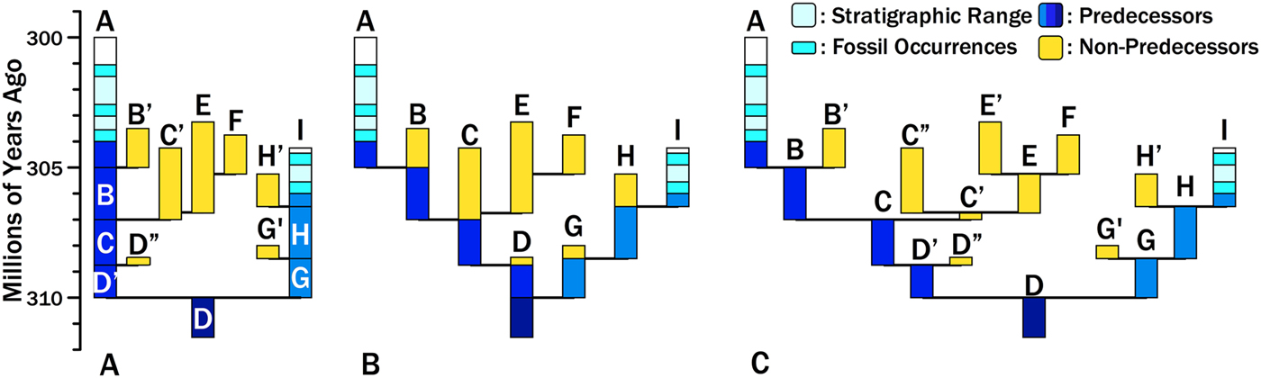
Figure 1. Hypothetical phylogeny for sampled lineages (black/light blue), unsampled predecessors (dark gray/dark blue), and unsampled sister taxa (light gray/yellow). A, Two sampled species diverged from unsampled Species D at 310 Ma, generating branch durations (and chronostratigraphic gaps) of 6 Myr for Species A and 4 Myr for Species I. Increased sampling will provide earlier divergence times and shorter branch durations/chronostratigraphic gaps in one of two ways. We might sample predecessors of A or I (dark gray/dark blue). The probability of doing so is the probability of sampling an individual lineage at any one point in time. Alternatively, we might sample sister taxa of A or I (light gray/yellow). The probability of doing so reflects origination (affecting the number of possible sister taxa and the richness of sister clades), extinction (affecting the richness of sister clades and the probability of sampling individual lineages), and sampling (affecting the probability of sampling individual lineages). B, The phylogeny re-rendered as budding speciation. Each letter represents a distinct morphospecies that we would recognize before phylogenetic analysis. Note that the predecessors of A and I now are only part of the durations of ancestors such a Species B and Species H. However, the sum of predecessors (dark gray/dark blue) and the sum of possible “sisters” (light gray/yellow) remains unchanged. C, The phylogeny re-rendered as bifurcation speciation, with ancestral morphospecies being at least slightly altered at divergence so that Species B and Species B′ have at least one character distinguishing them. Now predecessors and ancestors are nearly synonymous, save for the earliest unsampled members of Species A and I. However, the sum of predecessors and the sum of possible sisters remains unchanged.
As Bapst (Reference Bapst2013) emphasizes, the probability of any divergence time (and its implicit branch duration and stratigraphic gap within a phylogeny) reflects three rates: origination, extinction, and sampling rates. Origination and extinction both have two effects on this probability. Origination rates provide the expected number of cladogenetic events along any branch leading to the base of the tree. Both origination and extinction affect the expected number of progeny that any one cladogenetic event will ultimately generate: as origination increases and/or extinction decreases (i.e., as net diversification increases), we expect more taxa to evolve that could become sampled sister taxa. That in turn reduces the probability of deep divergences by increasing the probability of finding at least one descendant of a divergence, even if sampling rates themselves do not increase. Decreasing extinction has a similar effect, as increasing the durations of individual species increases the probability that at least one descendant of a divergence is found, even if neither origination nor sampling increase (Foote Reference Foote1996). Figure 1 illustrates how diversification affects expected branch durations and divergence times. There are three branching events leading to Species A compared with only two branching events leading to Species I; thus, all else being equal, it is more probable that subsequent sampling will add a sister taxon to Species A rather than to Species I. Moreover, one of Species A's possible sisters, the C+E+F clade, offers many more opportunities for sampling than do any of the other divergences. All else being equal, the probability of sampling some descendant of that “C” divergence is greater than the probability of sampling descendants of any other divergence.
These expectations are independent of particular speciation models. Re-rendering Fig. 1A as either a budding (Fig. 1B) or bifurcating (Fig. 1C) speciation model leaves the same branch durations leading from Species A and Species I to the base of the tree, and the same sum of durations for additional potential sister taxa. The difference is that “predecessors” and “ancestors” are basically identical given bifurcation, because ancestral morphotypes anagenetically change at cladogenesis, whereas predecessors include only those members of an ancestral species extant before cladogenesis under the budding model. (Under both models, the earliest members of Species A and Species I also are “predecessors.”) Under the latter model, the probability of sampling an ancestor is greater than the probability of sampling a predecessor (Foote Reference Foote1996). To avoid implying that ancestors necessarily become pseudoextinct at speciation, I will use the term “predecessor” for the analogues of the dark gray (dark blue online) bars in Fig. 1 throughout this paper.
Bapst (Reference Bapst2013) and Didier et al. (Reference Didier, Fau and Laurin2017) extend the work of Foote et al. (Reference Foote, Hunter, Janis and Sepkoski1999) by deriving the probability of sampling a species or any successors (i.e., a clade of unknown size) given time-homogeneous origination, extinction, and sampling. These birth–death-sampling models (= fossilized-birth–death sampling sensu Heath et al. Reference Heath, Huelsenbeck and Stadler2014; Gavryushkina et al. Reference Gavryushkina, Heath, Ksepka, Stadler, Welch and Drummond2016; Zhang et al. Reference Zhang, Stadler, Klopfstein, Heath and Ronquist2016; Stadler et al. Reference Stadler, Gavryushkina, Warnock, Drummond and Heath2018) offer great potential as tools for assessing the branch durations and divergence times implicit to rival phylogenetic hypotheses, and thus for assessing different models of anatomical evolution favoring those rival phylogenetic hypotheses. Moreover, because we have abundant paleobiological methods for estimating origination, extinction, and sampling from the fossil record, this represents a relatively rare case in which we can empirically justify the rate parameters that we need to estimate prior probabilities of branch durations and divergence times in Bayesian analyses.
The same paleobiological methods that provide us with diversification and sampling rates also indicate that all three rates all vary over time (e.g., Connolly and Miller Reference Connolly and Miller2001; Foote Reference Foote2001, Reference Foote2003; Liow and Finarelli Reference Liow and Finarelli2014; Alroy Reference Alroy2014; Finarelli and Liow Reference Finarelli and Liow2016). What we require to accommodate interval-to-interval variation in origination, extinction, and sampling is a general model that will estimate: (1) the probability of a species appearing in some interval generating any sampled specimens either of itself or some descendant species given the diversification and sampling rates of that interval and when in that interval the first species originated; (2) the probabilities that the first species sends 1…∞ successors (with the successors possibly including the first species itself) into the next interval given the origination and extinction rates of that first interval; and (3) the probability that any of those successors generate at least one sampled species given the origination, extinction, and sampling rates of subsequent intervals.
Table 1. Glossary of terms and variables of importance in this work.

The Probability of Sampling a Species or Any Successors from Any One Interval
In Figure 1, we posit that Species A and Species I are each other's closest sampled relative. The divergence time demands a branch duration and stratigraphic gap over which we failed to sample any specimens and over which no other sampled relatives diverged. If diversification and sampling rates are constant, then the expected number of sampled species or clades that should be more closely related to Species A than is Species I is Φλd, where λ is the origination rate, Φ is the proportion of branching events for which any successors are sampled (i.e., the probability of sampling a clade of unknown size sensu Bapst [2013]), and d is the branch duration leading to Species A (Table 1). Φ reflects sampling (ψ) and the summed species durations (S) expected given λ and μ (Foote et al. Reference Foote, Hunter, Janis and Sepkoski1999). For example, the C′+E + F clade (Fig. 1A) has S = 7.75 lineage million years (LMyr). Bapst (Reference Bapst2013: eq. 2) extends this logic to estimate the probability of sampling a species or any successors (i.e., a clade of unknown size) given constant λ, μ, and ψ as:
 $$\; \Phi = 1-\mathop \sum \limits_{K\; = \; 1}^\infty \displaystyle{{{\rm \lambda} ^{\lpar {K-1} \rpar }{\rm \mu} ^K\left( {\matrix{ {2K-2} \cr {K-1} \cr}} \right)} \over {K{\lpar {{\rm \lambda} + {\rm \mu} + {\rm \psi}} \rpar }^{\lpar {2K-1} \rpar }}}$$
where K = 1…∞ represents the possible richness generated by any one divergence. Didier et al (Reference Didier, Fau and Laurin2017: appendix 5; see also King in Bapst Reference Bapst2016) estimate Φ using a quadratic:
 $$\Phi= 1-\displaystyle{{\lpar {{\rm \lambda} + {\rm \mu} + {\rm \psi}} \rpar -\sqrt {{\lpar {{\rm \lambda} + {\rm \mu} + {\rm \psi}} \rpar }^2-4{\rm \lambda \mu}}} \over {2{\rm \lambda}}} $$
Bapst's and Didier et al.’s equations generate very similar estimates of Φ, and in both cases the probability of sampling a species or any successors increases as:
1. λ increases (increasing S by generating more species);
2. μ decreases (increasing S by generating longer-lived species);
3. ψ increases (increasing the probability of sampling per LMyr).
To estimate Φ given shifting diversification and/or sampling, we first need to estimate Φ′, the probability of sampling a clade of unknown size over some interval i of duration T i with its rates of λi, μi, and ψi. (Note that time now refers to time elapsed after a divergence, not time before a first appearance or the splitting from a common predecessor.) First, we calculate the probability that one lineage will result in K = 0…∞ lineages at any time from t = 0…T (Fig. 2). When λ ≠ μ:
 $$P{\rm [}K\; = \; 0\; {\rm \vert \lambda}, {\rm \mu}, t]\; = \; \displaystyle{{{\rm \mu} \times (e^{\lpar {{\rm \lambda} -{\rm \mu}} \rpar t}-1)} \over {\lpar {{\rm \lambda} \times e^{\lpar {{\rm \lambda} -{\rm \mu}} \rpar t}} \rpar -{\rm \mu}}} $$
Figure 2. The probability of there being K = 0…4 successors of a species extant at time t = 0 over an interval with duration T = 2.5 given different combinations of origination (λ) and extinction (μ) rates. Note that rates increase by a factor of 1.414 (20.5) between adjacent frames. Note that the successors might include the original species at any point in time.
(Raup Reference Raup1985: eq. A13) and
 $$\eqalign{P\lsqb {K \ge 1{\rm \vert \lambda}, {\rm \mu}, t} \rsqb \; & = \; \left( {1-\displaystyle{{{\rm \mu} \times (e^{\lpar {{\rm \lambda} -{\rm \mu}} \rpar t}-1)} \over {\lpar {{\rm \lambda} \times e^{\lpar {{\rm \lambda} -{\rm \mu}} \rpar t}} \rpar -{\rm \mu}}}} \right)\; \cr & \times \left( {1-\displaystyle{{{\rm \lambda \times \mu} \times {\rm \;} (e^{\lpar {{\rm \lambda} -{\rm \mu}} \rpar t}-1)} \over {{\rm \mu} \times \lpar {\lsqb {{\rm \lambda} \times e^{\lpar {{\rm \lambda} -{\rm \mu}} \rpar t}} \rsqb -{\rm \mu}} \rpar }}} \right) \cr &\times \left( {\displaystyle{{{\rm \lambda \times \mu} \times (e^{\lpar {{\rm \lambda} -{\rm \mu}} \rpar t}-1)} \over {{\rm \mu} \times \lpar {\lsqb {{\rm \lambda} \times e^{\lpar {{\rm \lambda} -{\rm \mu}} \rpar t}} \rsqb -{\rm \mu}} \rpar }}} \right)^{K-1}} $$
(Raup Reference Raup1985: eq. A13, A17). When λ = μ:
 $$P{\rm [}K\; = \; 0\; {\rm \vert \lambda}, {\rm \mu}, t]\; = \; \displaystyle{{{\rm \lambda} t} \over {1 + {\rm \lambda} t}}$$
(Raup Reference Raup1985: eq. A12), and
 $$P{\rm [}K \ge 1\; {\rm \vert \lambda}, {\rm \mu}, t]\; = \; \displaystyle{{{\lpar {{\rm \lambda} t} \rpar }^{K-1}} \over {{\lpar {1 + {\rm \lambda} t} \rpar }^{K + 1}}}$$
(Raup Reference Raup1985: eq. A14). Figure 2 illustrates these in nine combinations of rates over some interval with T = 2.5. Both λ and μ give expectations over t = 1 (e.g., rates per million years for an interval of 2.5 Myr).
Integrating over the individual probability curves for K successors of one species gives the E[t K], the expected amount of time within interval i in which K successors of the original species are present (Fig. 3). We can use this to estimate E[S], the expected sum of durations within an interval:
 $$E\lsqb S \rsqb \; = \; \mathop \sum \limits_{K\; = \; 1}^\infty \lpar {K \times E\lsqb {t_K} \rsqb } \rpar $$
that is, the number of lineages (K) times the expected time with that number of lineages (E[t N]) summed over all possible K. (Because E[t K] rapidly declines to very low numbers, the summation can be quickly truncated.) If we have Interval A with λ = μ = 0.4 Myr−1 (Fig. 3A), then:
 $$\eqalign{& {\rm E}\lsqb {S_A} \rsqb {\rm} = {\rm} (1{\rm \times} 1.250){\rm} + {\rm} (2{\rm \times} 0.625){\rm} + {\rm} (3{\rm \times} 0.313){\rm} \cr & \qquad \quad \,+ {\rm} (3{\rm \times} 0.156){\rm} + {\rm} (4{\rm \times} 0.078){\rm} \ldots \cr & = {\rm} 2.5{\rm}\ {\rm LMyr}} $$
Figure 3. The expected time with K = 0…4 successors (including the original species) given interval duration T = 2.5. These are the areas under each curve for the corresponding K, origination (λ) and extinction (μ) in the corresponding panels in Fig. 2. The sum of expected lineage durations, S, is the sum of K × E[T K]. Thus at λ = 0.4 and μ = 0.4 (A), E[S] = (1 × 1.25) + (2 × 0.313) + (3 × 0.104) + (4 × 0.039) … = 2.5 LMyr.
If we have Interval B with λ = 0.566 and μ = 0.4 (Fig. 3B), then:
 $$\eqalign{ {\rm E}\lsqb {S_B} \rsqb {\rm}& = {\rm} (1{\rm \times} 1.125){\rm} + {\rm} (2{\rm \times} 0.716){\rm} + {\rm} (3{\rm \times} 0.456){\rm} \cr & \quad+ {\rm} (3{\rm \times} 0.290){\rm} + {\rm} (4{\rm \times} 0.185){\rm} \ldots \; \cr & = {\rm} 3.1{\rm} \;{\rm LMyr}} $$
A first approximation of the probability of sampling a lineage present at the outset of any interval X or any successors to that species is:
 $${\rm \Phi} _X^{\prime} \; = \; 1-e^{-\psi _XE\lsqb {S_X} \rsqb }$$
Therefore, if ψA < 1.24 × ψB, then we expect to sample more clades diverging at the onset of Interval B than we would for Interval A.
Simulations show that eq. (7) overestimates Φ′. At λ = μ = ψ = 0.4 and T = 2.5, eqs. (6 and 7) estimate Φ′ = 0.632, whereas simulations starting using these same parameters generate sampled species in only 53.3% of runs (see also Supplementary Fig. S1). The culprit is the failure of eq. (6) to account for total extinction within the interval eliminating any possibility of additional sampling regardless of the remaining expected S (see Supplementary Fig. S2). One solution is to divide intervals into m interval-slices so that each per-slice ψ is low and then estimate: (1) νi, the probability of a species extant at the outset having sampled members or successor in interval-slice i (eq. 7); and (2) ζi, the probability of a lineage present at the outset of interval-slice i having sampled successors in interval-slices i + 1 to m. The former parameter, ν, is the probability of finding a species and/or any successors in an interval-slice:
 $${\rm \upsilon} _i\; = \; 1-e^{-{\rm \psi} _iE\lsqb {S_i} \rsqb t_i}$$
where ψi is the sampling rate for the interval, S i is the expected total progeny in the interval-slice, and t i is duration of the interval-slice. The latter parameter, ζ, is the probability of K = 1…∞ total progeny yielding at least one sampled species times given “future” λ, μ, and ψ multiplied by the probability of the initial species having K = 1…∞ successors (again, possibly including the original species) at the end of the interval-slice i given λi and μi (Fig. 4):
 $$ \eqalign{ \zeta _i\; = & \; \sum\nolimits_{K\; = \; 1}^\infty {\lpar {P\lsqb { \ge 1\; {\rm Finds\;} \vert K,{\rm \Phi}_{i + 1}^{\prime}} \rsqb }} \cr & \times P\lsqb {K\; Successors\; \vert {\rm \lambda}_{i.},{\rm \mu}_i} \rsqb\rpar } } $$
Figure 4. The probability of a species extant at the outset of an interval with particular origination (λ) and extinction (μ) having K = 0…4 successors extant 0.25 Myr later. The probability of the species or any successor generating a sampled species in the subsequent 0.25 Myr is conditioned on the probability of K = 0…∞ survivors going into the next interval-slice.
For the final interval-slice m, ζm = 0, because there are no opportunities to sample successors later in the interval. Thus,  ${\rm \Phi} _m^{\prime} $ = νm, and we can solve ζ1…(m − 1) recursively. The maximum possible value for ζi is the probability of any successors surviving interval-slice i: at λ = μ = 0.4 and T i = 0.25, the probability of extinction is 0.091 (Fig. 5A) and the maximum possible ζi is 0.909. Now:
 $${\rm \Phi} _i^{\prime} \cong 1-\lpar {\lsqb {1-\upsilon_i} \rsqb \times \lsqb {1-\zeta_i} \rsqb } \rpar $$
Figure 5. The effect of interval-slice length on overestimate of Φ′. Horizontal bars denote expected Φ′ given 5000 simulations at the appropriate origination (λ) and extinction (μ) rates. Intervals durations are set to T = 2.5, so at m = 250 slices, each t i = 0.001. See also Supplementary Fig. S3.
This explicitly accommodates the probability that a lineage present at the outset of an interval is extinct with no successors by (say) the 5th of m = 10 interval-slices.
Simulations (Fig. 5, Supplementary Fig. S1) show that eq. (9) rapidly converges to appropriate estimates of  ${\rm \Phi} _1^{\prime} $ at m ≥ 10 over the range of diversification parameters used in Figures 2–5. Thus, if we typically have intervals of (say) 2.5 Myr over which we have estimates of λ, μ, and ψ, then 100 kyr interval-slices should be adequate to estimate ${\rm \Phi} _1^{\prime} $.
Another useful aspect of calculating  ${\rm \Phi} _i^{\prime} $ for multiple slices within an interval is that divergences could happen at any time within an interval if origination is continuous through time. Suppose that the precision of divergence dates that we will consider are in 100 kyr increments: that is, we will ask whether a divergence happened at 450.1 Ma, 450.0 Ma, 449.9 Ma, etc. If these divergences are within a 2.5 Myr chronostratigraphic interval, then we then we need to know ${\rm \Phi} _{1 \ldots 25}^{\prime} $. ${\rm \Phi} _i^{\prime} $ will decrease as i increases: we have both less time to accrue lineage durations and less time in which to sample them. If the interval has λ = μ = ψ = 0.4 Myr−1, then: ${\rm \Phi} _1^{\prime} $ = 0.536, ${\rm \Phi} _{13}^{\prime} $ = 0.383, and ${\rm \Phi} _{25}^{\prime} {\rm \;} $= 0.039. Thus, even if the probability of a divergence is the same at any point within the interval, the probability of a divergence that generates a sampled species within that interval declines over time.
The Probability of Sampling a Species or Successors over 2+ Intervals with Different Diversification and/or Sampling Rates
The exercise above applies sampling within one interval. However, this is just the particular case where all m diversification and sampling rates are the same and ν1 = ν2… = νm. We can calculate eq. (9) just as easily using ν1 ≠ ν2… ≠ νm, as will be the case if either of the diversification rates or the sampling rate varied in every interval-slice. Similarly, ζi is just as easy to calculate if λi and/or μi differ in every interval-slice. What I will do here is intermediate: interval-slices from different intervals will use particular values of λ, μ, and ψ so that each ν i within an interval is identical and each ζi within an interval uses the same values of λ and μ. The one difference is that ζm will be greater than zero for all intervals save the last, and all ζi from those intervals will reflect subsequent shifts in diversification and/or sampling.
Suppose that we are analyzing a clade of Ordovician gastropod species known through the Katian. Suppose further that data from the Paleobiology Database coupled with an external stratigraphic database allow us to estimate separate diversification and sampling rates for gastropods as a whole for three divisions of the Katian, corresponding to Bergström et al.’s (Reference Bergström, Chen, Gutiérrez-Marco and Dronov2009) Ka1, Ka2 + Ka3 (hereafter: Ka2–3), and Ka4: λKa1 = 0.269, λKa2–3 = 0.348, λKa4 = 0.312; μKa1 = 0.293, μKa2–3 = 0.495, μKa4 = 0.514; and, ψKa1 = 0.147, ψKa2–3 = 0.155, ψKa4 = 0.122 (Fig. 6). These parameters come from capture-mark-recapture analysis (Connolly and Miller Reference Connolly and Miller2001; Liow and Nichols Reference Liow, Nichols, Alroy and Hunt2010) using Paleobiology Database data, with the analysis modified to allow for log-normal distributions of sampling rates (Wagner and Marcot Reference Wagner and Marcot2013) and each ψKa the median of those log-normal distributions. Each 100 kyr interval-slice within any one interval will have the same probability of a divergence in that interval-slice being sampled immediately: νi•Ka1 = 1.46 × 10⁻², νi•Ka2–3 =1.53 × 10⁻², νi•Ka4 = 1.20 × 10⁻² (Fig. 6A). Each 100 kyr interval-slice within an interval also shares the same probability of a species present at the outset having 0…∞ successors at the outset of the next 100 kyr interval-slice (Supplementary Fig. S3). However, ζi for a Ka2–3 divergence (i.e., the probability of sampling the species or successors in subsequent interval-slices) now reflects diversification and sampling in both Ka2–3 and Ka4 (Fig. 6). This in turn means that we now have Φi for each interval-slice within all three intervals: that is, the probability of ever sampling a descendant of a divergence occurring in that 100 kyr interval-slice at some point in the time range encompassed by our study. Simulations using the same origination, extinction, and sampling rates per interval indicate that eqs. (7a) and (8) combined generate accurate estimates of Φi for all interval-slices (Supplementary Fig. S4). This in turn indicates that eq. (6) is accurately estimating E[S] (expected summed durations evolving from a divergence) for different interval-slices given heterogeneous λ and μ.
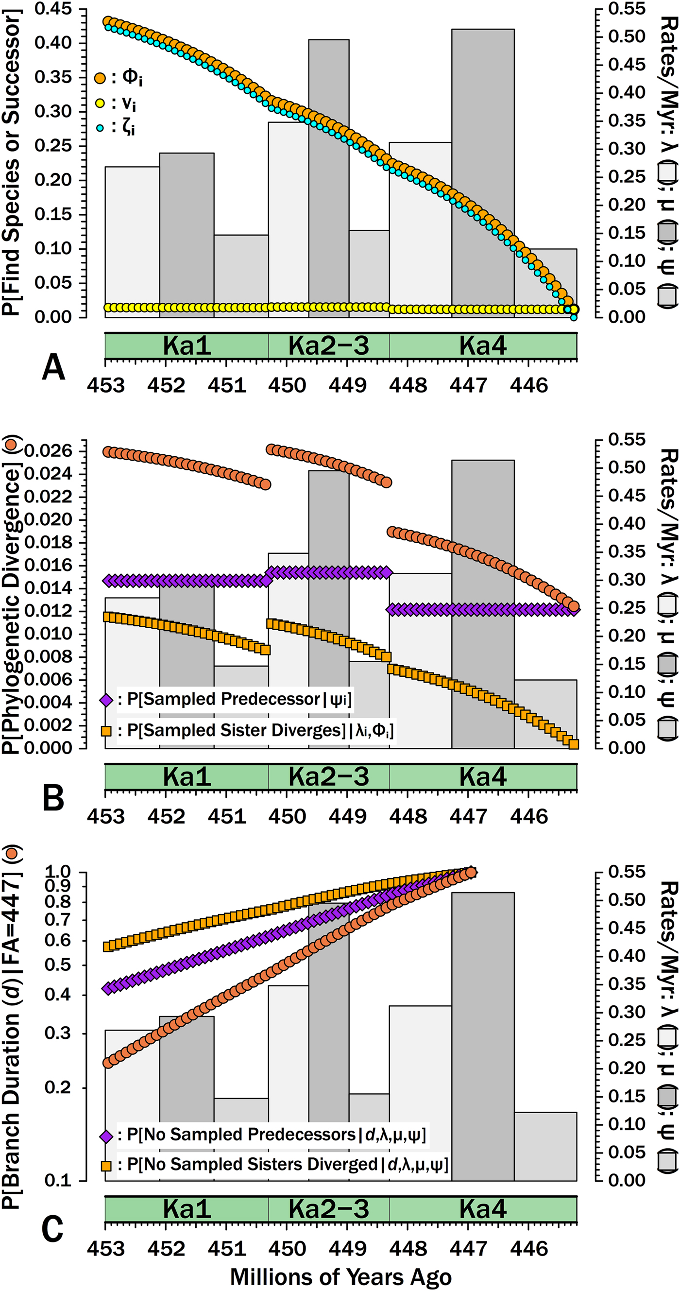
Figure 6. Breaking down estimates of branch duration probabilities given empirically estimated rates of origination (λ), extinction (μ), and sampling (ψ). Gray bars give rates for each interval (2nd y-axis). A, The components of Φi, the probability of sampling a species appearing in interval-slice i or any successors of that species (i.e., a clade of unknown size). νi (yellow dots) gives the probability of sampling that species or any successors in interval-slice i. ζi (light blue dots) gives the probability of sampling any successors of that species (including the original species) in interval-slice i + 1 or any time afterward before the end of the Katian. Φi reflects the probability of doing either and therefore is Φi = 1− ([1 − νi] × [1 − ζi]). B, The exact probability of a branch duration leading to a sampled species or to a node linking sampled species starting in interval-slice i. The probability of sampling a predecessor (purple) is the probability of sampling the one predecessor of a species or node extant in interval-slice i. The probability of sampling a sister taxon (dark orange) is the probability of a divergence giving rise to a sister taxon with 1+ sampled species in interval-slice i. The probability of one or the other happening (sienna) is the probability of a phylogenetic divergence in interval-slice i given that we have some sampled species with a first occurrence after interval-slice i (or a node linking sampled species that diverges after interval-slice i). C, The probabilities of branch durations (sienna) preceding Salpingostoma richmondensis, which is first known from early in the Aphelognathus divergens conodont Zone. This is broken down into the probability of duration d with no divergences to sampled sister taxa (orange) and the probability of no sampled precursors (purple). The expected branch duration (where P[d] = 0.50) is 3.2 Myr.
The Probability of Branch Durations and Divergence Times Given Shifting Rates of Diversification and/or Sampling
We now can estimate the probability that a branch duration leading to a sampled species (or to the basal divergence of a sampled clade) diverges from the rest of the clade in any particular interval-slice. Following the gastropod example above, suppose that we are analyzing a group of bellerophontoids through the Katian. One of the species is Salpingostoma richmondensis, which is first known from rocks at the base of the Aphelognathus divergens conodont Zone in Ka4. What is the probability that S. richmondensis diverged from its closest relative before the Katian? Based on Gradstein et al. (Reference Gradstein, Ogg and Schmitz2012), we assign an earliest appearance date of 447 Ma for S. richmondensis, that is, about halfway through Ka4. (I will disregard uncertainty in the time-scale here.) Given that the Katian starts at 453 Ma, we are positing a minimum branch duration of d = 6 Myr. The probability of failing to sample a predecessor of S. richmondensis over d = 6 Myr is the probability of missing it in every interval-slice i:
 $$e^{-\sum\nolimits_{i\; = \; 1}^{FA-1} {{\rm \psi } _id_i}} $$
where FA-1 is the interval-slice preceding the first appearance (here, the interval-slice corresponding to 447.1 Ma), d 1 is the time encompassed by each interval-slice (here, 100 kyr), and ψi is the sampling rate of that interval. (Fig. 6B gives the complement of this, i.e., the probability of sampling a predecessor per interval-slice). Given the sampling rates from above, this comes to p = 0.420.
The probability of there being no divergences leading to a sister taxon of S. richmondensis sampled in the Katian reflects the three separate origination rates and Φi at any given point in time:
 $$\mathop \prod \limits_{i\; = \; 1}^{FA-1} \mathop \sum \limits_{n\; = \; 1}^\infty \lpar {P\lsqb {n\; {\rm branchings} \vert \lambda_id_i} \rsqb \times {\lsqb {1-{\rm \Phi}_i} \rsqb }^n} \rpar $$
where P[n branchings|λi] is the Poisson probability of n cladogenetic events in an interval-slice given the origination rate of that interval and the duration of each interval-slice (here, 100 kyr), and [1-Φi]n is the probability of n divergences yielding no sampled sister taxa. Here, this generates p = 0.574. We usually will get almost identical results estimating the probability of no divergences leading to sampled sister taxa as:
 $$e^{-\sum\nolimits_{i\; = \; 1}^{FA-1} {{\rm \Phi} _i{\rm \lambda} _id_i}} $$
because the probability of just one branching event is nearly equal to the probability of there being any branching events. However, at origination rates comparable to those estimated for major radiations, the probability of two branching events over even short intervals is great enough that not allowing for n = 2 yields notable underestimates of the probability of a sampled sister taxon. (Note that even with very high λ, we can truncate the summation by n = 5.)
The complement of eq. (11) is the probability that any given interval-slice includes a divergence leading to a sampled sister taxon of S. richmondensis (Fig. 6B). This increases not just as Φ increases (Fig. 6A), but also as λ increases: thus, the probability of a divergence leading to a sampled sister taxon of S. richmondensis peaks early in Ka2–3, despite the edge effect of ending the study after the next interval (Fig. 6B). Because ψKa2–3 is only marginally higher than ψKa1 and ψKa4 is less than ψKa1, this necessarily is driven by the λKa2–3 being greater than λKa1. The combination of elevated λ and elevated ψ in Ka2–3 also means that these interval-slices have the highest probabilities of providing S. richmondensis’s divergence from either a sampled predecessor or a sampled sister taxon.
We now calculate the probability of branch duration d as the probability of no sampled predecessors (i.e., one minus eq. 10) times the probability of no divergences leading to sampled sister taxa (i.e., one minus eq. 11). Thus, the probability that S. richmondensis has a divergence time from other bellerophontoids no later than the base of the Katian given the shifting diversification and sampling rates of the Katian (and without the possibility of sampling post-Katian sister taxa) is 0.420 × 0.574 = 0.241 (Fig. 6C). Finally, note that if we do not include any post-Katian species, then the expected branch duration for S. richmondensis (E[d]), that is, the point where the probability of the branch duration is 0.5, is 3.1 Myr.
Effects of Simple Shifts in Sampling and/or Diversification Rates on Expected Stratigraphic Gaps and Branch Durations
The specific effects of each parameter are difficult to appreciate when origination, extinction, and sampling all vary from one interval to the next, as in the Katian gastropod example. Moreover, the short span of time encompassed by the Katian data creates a major edge effect: Φi steadily declines throughout the Katian because no post-Katian descendants of Katian divergences can be sampled. Most studies include many more than one stage and thus might have many intervals without such an edge effect. Indeed, just how long before the conclusion of a study (or before the total extinction of a clade) we need to go before this edge effect disappears is in itself a question of interest.
Therefore, I will present simple examples in which (with one exception) two of the rate parameters are held constant while one varies over time. This will emphasize how the particular parameters affect the probabilities of branch durations and divergence times. I will first cover shifts in sampling with constant diversification. I then will cover some simplified versions of major evolutionary events given constant sampling. The latter examples are particularly important, not simply because they emphasize the strong effects of both origination and extinction rates on expected branch durations and stratigraphic gaps within a phylogeny, but because paleobiologists often target species spanning such events when conducting phylogenetic analyses. In each example, I will use 6 intervals of 2.5 Myr each, with estimates of Φ based on 100 kyr interval-slices. The “standard” diversification rates are set to 0.4 Myr−1 so that we expect one event per interval. In all cases, I will use different median sampling levels that range from an expectation of one sample per interval to one sample per 100 intervals. To avoid the edge effect from the Katian gastropod example, all of the examples (save one) are followed by 12 intervals with “normal” λ, μ, and ψ.
For each combination of parameters and parameter shifts, I present the following: (1) Φ, the probability of sampling a species or any successors (= a clade of unknown size); (2) the probability of a divergence leading to a sampled sister taxon given expectation λiΦi; (3) the probability of truncating a branch duration in interval-slice i either by sampling a predecessor or from the divergence of a subsequently sampled sister taxon; and (4) the expected branch duration (E[d]) given a sampled species with that first appears in interval-slice i. The last represents the branch duration where the probability of encountering either a sampled predecessor or the divergence time of a sampled sister taxon reaches 0.5. Note that this E[d] also applies to the expected branch duration leading to a node that diverges in interval-slice i.
Finally, for Φ over time, I also include the results from 10,000 simulations (dots in Figs. 7A, 8). Each simulation begins with a single lineage, with both lifetimes and descendants per time-slice allowing for shifts in either diversification or sampling. Lifetimes and progeny of descendants are simulated the same way, albeit using rates specific to their lifetimes. Interval-specific rates of sampling are used when sampling changes. The results show the proportion of simulated lineages that generate 1+ sampled species.
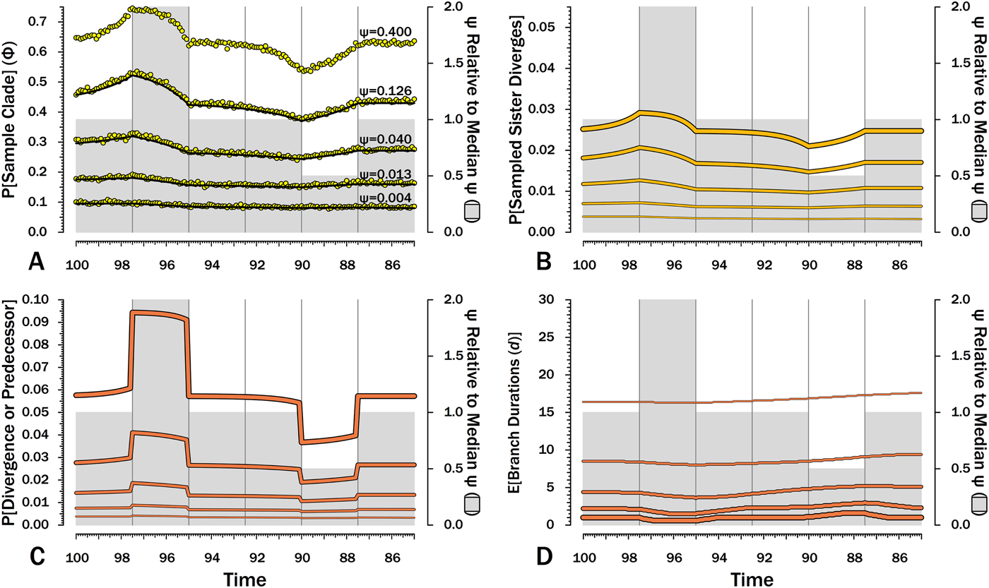
Figure 7. Effects of variable sampling over time with constant origination and extinction (λ = μ = 0.40). Five median sampling rates (ψ) are illustrated, with ψ relative to the median given on by the gray bars (2nd y-axis). The six intervals of 2.5 Myr are preceded by six others with median ψ. A, Φ, the probability of sampling a species or any successors given that the species is extant in an interval-slice. Yellow dots give expected Φ given 10,000 simulations using ψ (and λ and μ) of the intervals of a species lifetime. B, The probability of a sampled sister species diverging in each interval-slice. C, The probability of a phylogenetic divergence in each interval-slice from either sampling a predecessor or from the divergence of a subsequently sampled sister taxon. D, Expected durations (d) for a species first appearing in each interval-slice. This also applies to a node that diverged in the same interval-slice. E[d] is the branch duration where P[no ancestors or divergences] reaches 0.50 (see Fig. 6C).
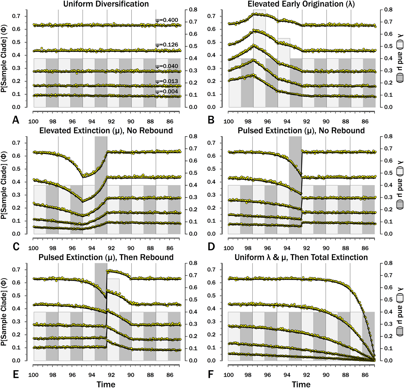
Figure 8. Probabilities of sampling clades of unknown size (Φ) under exemplar models of diversification. Origination, extinction, and sampling rates are per millions of years, with each interval 2.5 Myr long. Each Φi is for a 100 kyr slice. Black lines indicate Φ based on text eq. (9) and the rates of origination (λ, in light gray) and extinction (μ, in dark gray) of that time-slice and subsequent time-slices. For each curve, one of five sampling rates (ψ) is assumed for the entire duration. For pulsed extinction, the gray bar shows the average stage rate, with μi = 0.4 for the first 24 slices and μi = 10.4 for the final interval-slice, giving average μ = 0.8. Yellow dots represent the results of 10,000 simulations and give the proportion of runs in which a lineage appearing at that time ultimately generates a sampled specimen given subsequent diversification.
Effects of Shifts in Sampling Rates (ψ)
Although there are several evolutionary scenarios positing general shifts in origination and/or extinction rates, temporal patterns in sampling rates (ψ) do not have analogous simple models. The biggest control on ψ is the amount of available sedimentary rock from the right environmental type (Raup Reference Raup1972; Sheehan Reference Sheehan1977; Peters and Foote Reference Peters and Foote2001; Smith Reference Smith2001a), which can vary fairly haphazardly over time. In the absence of any such templates, I use two shifts in ψ, where one interval has twice the median sampling rates and another has half the median sampling rates (Fig. 7). A key feature is that the effects of shifts in sampling on the probability of sampling a species or any descendants (Φ) precedes shifts in ψ (Fig. 7A): compared with species appearing in other intervals, species appearing shortly before elevated sampling have a higher probability of surviving to and/or having descendants in the interval of high sampling even if they do not have elevated probabilities of numerous descendants and/or long durations. Conversely, Φ is depressed before the fourth interval, because species arising then have much lower probability of having descendants present during “normal” sampling intervals. We see the same patterns in reverse within the intervals of elevated and depressed ψ: Φ declines over the second interval, because species arising late in that interval have less time to generate descendants during the time of elevated sampling than do species arising early in the interval. Similarly, Φ increases over the fifth interval, because species arising late in the interval have a higher probability of having successors present during intervals of normal ψ. These patterns are mirrored in the actual probabilities of a sampled sister taxon arising in each interval-slice simply because λ is constant here (Fig. 7B). Finally, it is the absolute shifts in ψ that seem to be important: simply doubling low ψ has relatively little impact because 2ψ never is high enough in such cases to greatly improve the probability of a clade member being sampled before the clade becomes extinct.
The exact probability that an earlier-sampled species or clade diverges from other sampled members of the clade in any interval-slice reflects both ψ at that point in time (i.e., the probability of sampling a predecessor) and subsequent ψ (i.e., the probability of sampling a sister clade). The primary shifts (Fig. 7C) strongly reflect the changing probability of sampling a predecessor, particularly when ψ is high and the probability of a sampled predecessor or the divergence of a sampled sister taxon is high. However, changes in Φ in response to reduced ψ in later intervals cause the probability of a sampled divergence date to grade from one interval to the next, rather than simply be flat throughout an interval (see, e.g., Wagner Reference Wagner2000b). As above, this effect is muted when ψ is low, simply because absolute values are more important than relative values here.
When ψ is high, the expected branch durations (E[d]) increase or decrease rapidly around intervals of depressed or elevated sampling (Fig. 7) and then return to “normal.” When ψ is low, shifts in E[d] are extended over much longer period of time. Reduced sampling lengthens expected branch durations for taxa evolving well after the low-ψ interval, whereas elevated sampling reduces expected branch durations for taxa evolving well after the low-ψ interval. Indeed, at the lowest ψ used here, the effects of the elevated ψ interval on E[d] extend up to taxa appearing during (or just before) the low-ψ interval! This stated, the effects are fairly muted at low-ψ, at least when ψ varies by only factors of two. Finally, simulations indicate that our estimates of Φ accurately predict the probability of sampling at least one descendant of any given divergence when ψ varies, regardless of the typical rate.
Effects of Shifts in Diversification Rates (λ and μ)
I use five shifts in diversification rates to stereotype five basic macroevolutionary scenarios:
1. a burst of high speciation with constant extinction;
2. an interval of elevated continuous extinction and constant origination;
3. an interval ending with elevated pulsed extinction and constant origination;
4. an interval ending with elevated pulsed extinction followed by a rebound interval of elevated origination; and
5. sudden total extinction ending a clade.
I also include constant rates of λ and μ (Figs. 8A, 9A, 10A, 11A). This provides a comparison for assessing the importance of shifting rates and also allows comparison with both the Bapst (Reference Bapst2013) and Didier et al. (Reference Didier, Fau and Laurin2017) estimates of Φ (Table 2).
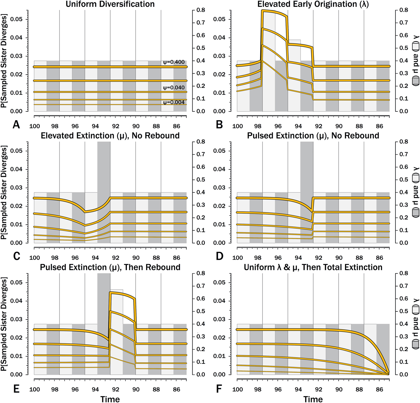
Figure 9. Probabilities of a divergence that ultimately generates a sampled species given the subsequent origination, extinction, and sampling rates.
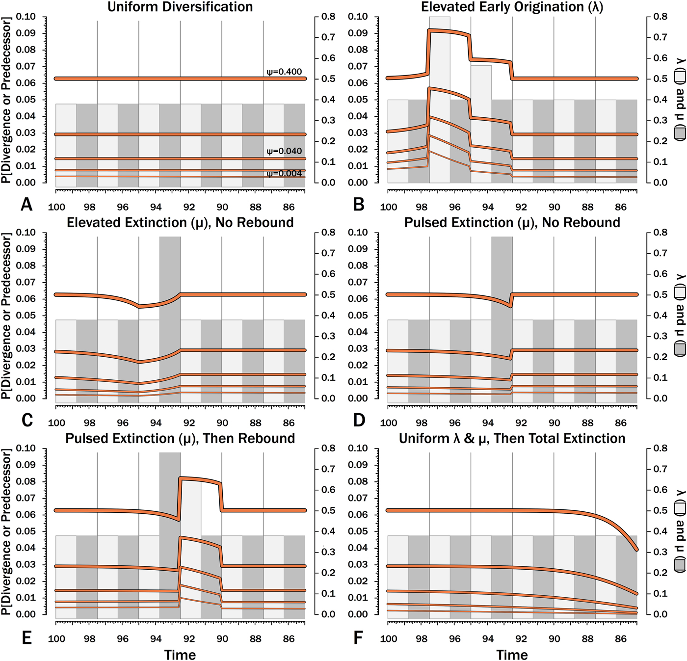
Figure 10. Probabilities of setting a phylogenetic divergence in a particular 100 kyr interval-slice, either by sampling a predecessor or by the divergence of a sister taxon that is sampled in that interval-slice or in some subsequent one. The complements of these probabilities are the probabilities of a stratigraphic gap within a phylogeny over the particular interval-slices. The product of these probabilities over any set of interval-slices gives the prior probability of a branch duration spanning that set of interval-slices.
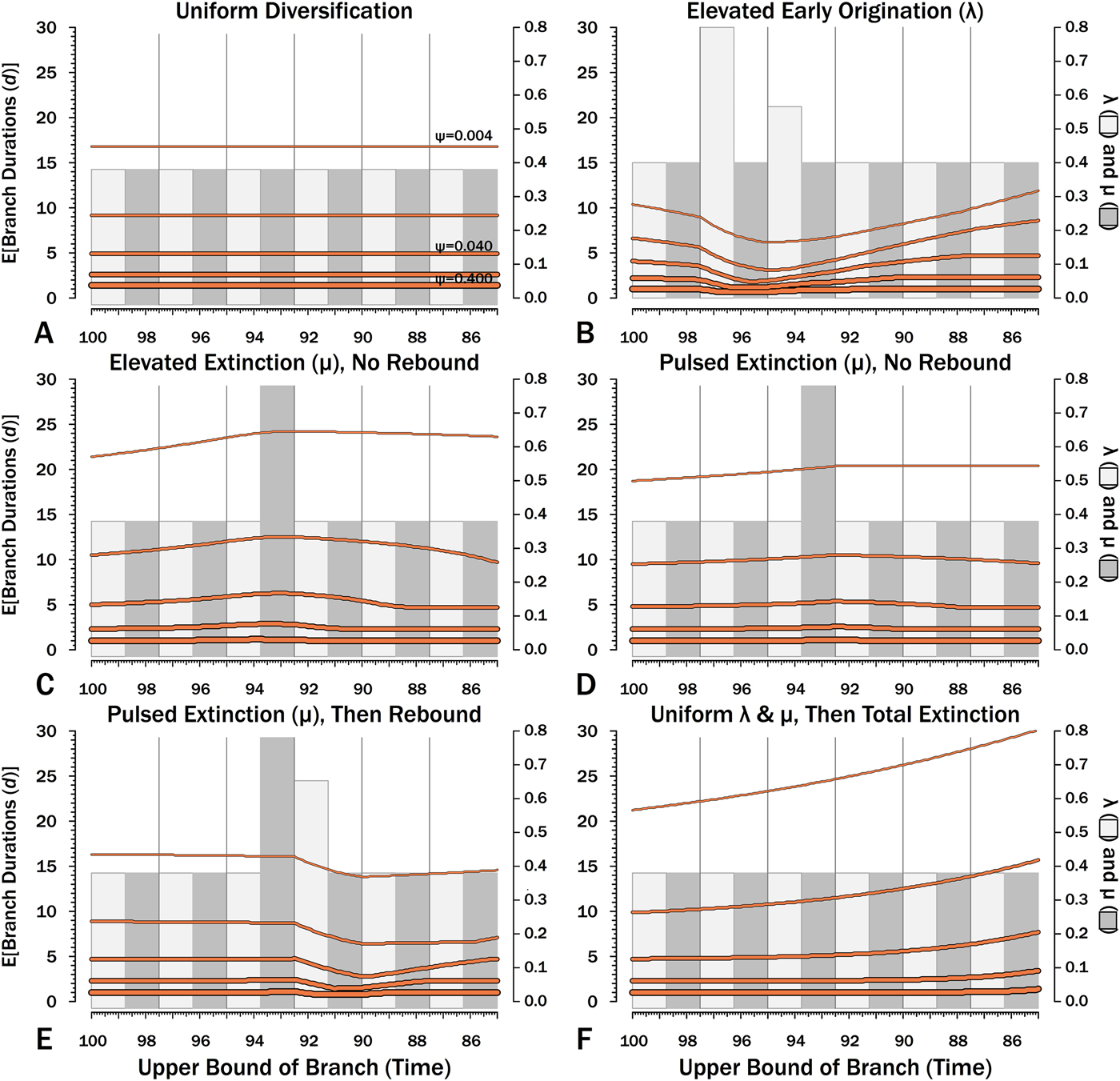
Figure 11. Expected branch durations (E[d]) for a species first appearing in an interval-slice or for an unsampled ancestor diverging in that interval-slice. E[d] is the branch duration where P[d|λ,μ,ψ] = 0.5. Note that E[d] at low ψ allows for several preceding intervals with “normal” diversification and sampling rates.
Table 2. The probability of sampling a clade of unknown size given origination and extinction = 0.4 and different levels of sampling (ψ). ΦB gives the global estimate for a clade given Bapst (Reference Bapst2013); ΦD gives the global estimate given Didier et al (Reference Didier, Fau and Laurin2017); and med. Φi gives the median 100 kyr estimate that allows for variation in diversification and sampling.

Constant Diversification and Sampling
When diversification and sampling are constant over time, the estimates of Φ that allow for temporal variation in diversification and sampling rates are nearly identical to estimates assuming constant rates (Table 2). The greatest difference is seen when ψ is very low. As discussed later, this reflects the fact that the edge effect of not allowing sampling 13+ intervals later begins to affect the probability of sampling sister taxa at very low levels of sampling.
Intervals of Elevated Origination
Here, λ doubles in the second interval, and then decreases by 1.414 times over both of the next two intervals to return to the “normal” level. Elevating λ raises Φ not just in the intervals of high λ, but also in preceding intervals (Fig. 8B). The latter effect becomes more pronounced as ψ decreases: at ψ = 0.4 (50% taxon sampling given μ = 0.4 and P[taxon sampling] =  $\displaystyle{{\rm \psi} \over {{\rm \mu} + {\rm \psi}}} $; Foote Reference Foote1996), Φ at the onset of the interval preceding diversification is close to that expected given normal rates (Fig. 8A); however, given ψ = 0.004 (~0.99% taxon sampling given μ = 0.4), Φ at the onset of the preceding interval is twice that expected given normal rates. Accordingly, the probability of a sampled clade diverging in the interval preceding a radiation is greater than the probability of a sampled clade diverging after that radiation, even if the origination rates themselves are the same before and after (Fig. 9B).
The effects of elevated λ on expected branch durations and stratigraphic gaps within a tree (E[d]) also are more dramatic when ψ is low than when ψ is high (Figs. 10B, 11B). When ψ is high, expected sampled predecessors make long branch durations and stratigraphic gaps improbable given either high or low λ (see, e.g., Foote Reference Foote1996). On the other hand, when ψ is low, divergence times usually are truncated by sampled sister taxa and the increased probability of sampled sister taxa when or before λ is high reduces expected branch durations. Thus, the effect of elevated λ on E[d] is more pronounced under low ψ than under high ψ.
Interval of Continuous Elevated Extinction
Here, μ is twice normal for one interval. Elevated μ causes both Φ and expected sampled sister taxa to decrease in the intervals leading up to it (Figs. 7C, 8C). This reflects the decreased probability of a lineage having numerous and/or long-lived progeny. As ψ decreases, the effect of elevated μ on Φ extends further back in time before the extinction interval. However, Φ increases as the extinction interval progresses, reflecting the increasing probability of extant species having surviving successors that might be sampled in subsequent intervals.
Intervals of elevated extinction increase the probability of stratigraphic gaps (Fig. 9C) and thus inflate expected branch durations and stratigraphic gaps for species first appearing either before or after the interval of extinction (Figs. 10C, 11C). This reflects the increased probability of sister taxa going extinct before generating a sampled species. The effect becomes more pronounced as ψ decreases and the probability of setting a divergence time with a sampled predecessor decreases: not only is E[d] higher during the extinction interval, but E[d] is also inflated in earlier and later intervals (Fig. 8C vs. 8A at the same ψ).
Interval Ending in Pulsed Elevated Extinction
There is considerable evidence that some major extinctions occur as pulses at the end of intervals (Marshall Reference Marshall1995a; Jin et al. Reference Jin, Wang, Wang, Shang, Cao and Erwin2000; Wang and Marshall Reference Wang and Marshall2004; Wang et al. Reference Wang, Sadler, Shen, Erwin, Zhang, Wang, Wang, Crowley and Henderson2014). Therefore, I model pulsed extinction here by setting μi = 10.4 for the final interval-slice and μi = 0.4 for the first 24 interval-slices. The probability of extinction for an individual species present at the outset of the high-extinction interval is the same as in the continuous elevated-extinction example (0.86), but with the bulk of the extinction concentrated in the final interval-slice. This generates a similar decline in Φ and expected sampled divergences as we see given elevated continuous extinction (Figs. 10D, 11D vs. 10C, 11C), but with the decline in Φ now shifted so that the minimum values are at the end of the extinction interval rather than at the outset. Correspondingly, the rebound to “normal” Φ and expected sampled divergences is immediate rather than protracted. The differences in both offset and the rebound reflect species appearing in the middle of the interval not having appreciably better probabilities of having surviving successors than species appearing or existing at the outset of the interval. The amount of time with depressed Φ before the extinction also is lower with pulsed extinction than with continuous extinction of the same magnitude, particularly when ψ is low. The effect on expected branch durations and stratigraphic gaps at any given sampling level ψ is muted under pulsed extinction relative to continuous extinction (Figs. 9D vs. 9C and 10D vs. 10C). Not only are the maximum deviations from “normal” lower, but the departures from normal begin and end closer to the extinction event.
Pulsed Elevated Extinction followed by Rebound in Origination
Intervals following elevated extinction often show rebounds with elevated origination (e.g., Miller and Sepkoski Reference Miller and Sepkoski1988; Lu et al. Reference Lu, Yogo and Marshall2006; Foote et al. Reference Foote, Cooper, Crampton and Sadler2018). The probability of sister taxa evolving in the last interval and then surviving the extinction are the same as in the prior example. However, there now is a much higher probability that any species evolving before the extinction that do have surviving successors will generate a sampled descendant, which dampens the drop in Φ (Figs. 8E, 9E vs. 8D, 9D). This results in a mixing of the expected phylogenetic patterns preceding extinctions and radiations: the extinction reduces the probability of sampled sister taxa diverging before the extinction and subsequent, which offsets the preradiation decrease in expected branch durations (Figs. 10E, 11E vs. 10B, 11E); however, the elevated probability of sampling the successors of any survivors dampens the expected increase in branch durations induced by the extinction (Figs. 10E, 11E vs. 10D, 11D). As in other scenarios, low ψ results in more time elapsing after the rebound before we return to “normal” branch durations and stratigraphic gaps. In particular, E[d] decreases going back in time (Fig. 11E) until the rebound interval, and then rapidly increases. Going further back in time, E[d] increases slightly rather than decreases (as expected when there is no rebound), with the time of increase greater at low ψ than at high ψ.
Complete Extinction (or End of Study Edge Effect)
Whole clades might go extinct during pulsed extinctions, which ends the chance to sample subsequent successors. For example, in a phylogenetic analysis of nonavian dinosaurs or ammonites from the Cretaceous, there is no opportunity for an unsampled Maastrichtian species to leave Paleocene or Eocene species that would document that particular divergence. Therefore, divergences that are not sampled in the Maastrichtian are never sampled. This has strong effects on branch durations. Even if λ, μ, and ψ are static before the extinction event, Φ declines markedly before the extinction (Fig. 8F). Because divergences generating sampled sister taxa become rarer (Fig. 9F), expected branch durations increase as taxon first appearances approach the extinction (Figs. 10F, 11F).
The effect of ψ on Φ and expected sampled sister taxa seen for elevated extinction rates above becomes even more pronounced given total extinction. Under high ψ, Φ begins to decline notably only about 1.5 intervals (= 1.5 times the average species duration) before the extinction. However, at the lowest ψ, Φ is only half of “normal” (Fig. 8F vs. 8A) six intervals (again, six times the average species duration) before the extinction. We see a corresponding effect on expected branch durations (Fig. 11F). When ψ is high, E[d] is low until just before the extinction: even though we have little chance of sampling late divergences in any way, we have a high probability of sampling the predecessors of those late-appearing species that we do sample. When ψ is low and we do not expect to sample many direct predecessors, E[d] just before the extinction can be nearly twice E[d] under the same “normal” diversification and sampling rates (Fig. 11E vs. 11A), simply because of our inability to sample survivors of the extinction.
The sudden extinction scenario here is the same as edge effect that excluding post-Katian species induces on the expected branch durations for an analysis of pre-Hirnantian gastropods only. As also noted earlier, this edge effect can be seen in Table 2. At the two lowest sampling levels, median Φ given homogeneous λ, μ, and ψ is lower when we allow for temporal variation than when we do not. At the second-lowest level (where we expect to sample about 3% of taxa), Φi drops below the “global” estimate over 18 intervals before the end of the calculations. At the lowest ψ, Φi is less than the estimates assuming constant diversification and sampling at least 30 intervals before the conclusion.
Discussion
Simulations illustrated in Figures 7 and 8 and Supplementary Figure S4 indicate that the approach here does well at predicting the probability of sampling a species and/or any of its descendants given “future” sampling and diversification. This reflects eq. (6) and its building blocks adequately converting λi and μi to S i, the expected summed durations of a lineage or clade members within an interval-slice. As this is the most complicated portion of estimating probabilities of unsampled branch durations, this gives us some confidence that the approach will work with real data using even more complex interval-to-interval variation in diversification and sampling. Therefore, I will discuss first some implications for tree-based studies, and then outline some further modifications that we can make to accommodate evolutionary scenarios not considered earlier.
Shifts in Net-Diversification Rates and Shifts in Sampling Rates Have Similar Effects on the Prior Probability of Sampled Sister Taxa
Comparing Figure 7 to Figures 8–11 corroborates a conclusion that necessarily follows from the works of Foote et al. (Reference Foote, Hunter, Janis and Sepkoski1999), Bapst (Reference Bapst2013), and Didier et al. (Reference Didier, Fau and Laurin2017): increasing net-diversification rates has the same general effect as increasing sampling rates, whereas decreasing net-diversification rates has the same general effect as decreasing sampling rates. The primary difference in how net diversification and sampling affect branch durations is that whereas both affect the probability of sampling sister taxa, only sampling rates affect the probability of sampling predecessors. A corollary to this is that the relative effects of shifts in diversification rates on expected branch durations and divergence times increase as overall sampling decreases: if sampled predecessors only infrequently terminate branch durations, then we require changes in λ and/or μ to increase or decrease the probability of sampling a sister taxon. Conversely, if we had 100% taxon sampling, then sister taxa would never set divergence times, as we would find all predecessors.
Phylogenetic Signor-Lipps Effect
Elevated extinction rates over short periods of time coupled with imperfect sampling create “gradual” series of last appearances in the fossil record (i.e., the Signor-Lipps effect; Signor and Lipps Reference Signor and Lipps1982; Raup Reference Raup1986). This extends to phylogenetic patterns: because elevated extinction decreases the probability that any descendant of a divergence will ever be sampled, we expect there to be fewer nodes on phylogenies leading up to major extinctions even if rates of λ, μ, and ψ are static up to that extinction. The magnitude of the effect increases both with the severity of the extinction and with the paucity of the fossil record. The latter is particularly important. Consider ammonites and nonavian dinosaurs, both of which are entirely eliminated by the K/Pg extinction. Because ammonites almost certainly have much higher ψ than do dinosaurs (Foote and Sepkoski Reference Foote and Sepkoski1999; Bapst et al. Reference Bapst, Wright, Matzke and Lloyd2016), we expect the K/Pg to induce less “distortion” in the branch durations and stratigraphic gaps within Cretaceous ammonite phylogeny than within Cretaceous dinosaur phylogeny (Figs. 8F, 9F, 10F, 11F).
Dinosaurs offer a possible warning case here. Sakamoto et al. (Reference Sakamoto, Benton and Venditti2016) note a decreasing frequency of nodes in nonavian dinosaur phylogeny through the latter half of the Cretaceous. They attribute this to prolonged decline in λ. However, we expect at least part of this to be due to the K/Pg extinction eliminating nonavian dinosaurs and creating a phylogenetic Signor-Lipps effect that reduces Late Cretaceous Φ and thus expected nodes among Late Cretaceous taxa. The question then becomes: How far back in time might this effect have stretched? Answering this requires first answering another question: What are typical sampling rates for dinosaur? Starrfelt and Liow (Reference Starrfelt and Liow2016) use the TRiPS method to estimate the overall sampling probability of dinosaur species to be greater than 0.5. As per-taxon sampling probability equals  $\displaystyle{{\rm \psi} \over {{\rm \mu} + {\rm \psi}}} $ (Foote Reference Foote1996), this implies that sampling rates exceed extinction rates and that any Signor-Lipps effect on phylogeny will be restricted to the latest Maastrichtian (Figs. 8F–11F). However, Bapst et al. (Reference Bapst, Wright, Matzke and Lloyd2016; see also Benson et al. Reference Benson, Hunt, Carrano and Campione2018) use Foote's (Reference Foote1997) method to estimate that dinosaur ψ is about 60 times lower than dinosaur μ. This is most comparable to the expectations given the lowest ψ used here. Bapst et al. estimated μ = 0.935, which in turn implies an average dinosaur species duration of 1.1 Myr. At the lowest sampling levels examined earlier, the phylogenetic Signor-Lipps effect extends back 30 times the average species lifetime. For dinosaurs, that would mean reduced sampling of sister taxa extending back over 30 Myr, that is, to the Campanian. Relative sampling could be even lower than that for dinosaurs. Distributions of ψ among contemporaneous mammal species follow log-normal distributions (Wagner and Marcot Reference Wagner and Marcot2013; see also Foote Reference Foote2016), and the sampling rates estimated by methods such Foote's Reference Foote1997 one typically are 10 to 100 times higher than median (= geometric mean) log-normal rates. If so, then the Signor-Lipps effect on Φ caused by the K/Pg extinction could be more severe than any case illustrated here. On the other hand, interest in extinction patterns leading up to the K/Pg might create unusually high ψ in the Maastrichtian, which in turn should increase the proportions of nodes found in the Late Cretaceous (see, e.g., Starrfelt and Liow Reference Starrfelt and Liow2016: Fig. 1). This would be similar to the “pull of the recent” (Raup Reference Raup1979) effect, in which the high sampling of extant taxa increases the representation of recent divergences on phylogenies (Heath et al. Reference Heath, Huelsenbeck and Stadler2014). Thus, assessing the effects of the total extinction of nonavian dinosaurs requires not just the typical sampling rates, but also the heterogeneity in those sampling rates over time.
Low Sampling Will “Blur” Radiations Back in Time
When using appearance or occurrence data, incomplete sampling has the same effect on the apparent timing of radiations as it does on extinctions, albeit in reverse, by making events look more gradual than they truly were (i.e., the Jaanusson effect or Sppil-Rongis effect; Jaanusson Reference Jaanusson and Bassett1976; Marshall Reference Marshall, Erwin and Anstey1995b, Reference Marshall, Paul and Donovan1998). However, sampling induces the opposite effect on the expected frequencies of sampled divergences (= nodes on a cladogram) during radiations, as we expect the frequency of nodes to increase before λ increases (Figs. 8B, 9B). As a corollary, the expected branch durations/stratigraphic gaps (E[d]; Figs. 10B, 11B) should decrease before λ increases.
The blurring effect becomes more pronounced as ψ decreases. To envision why this would be, suppose that we are examining two Ordovician echinoderm and brachiopod clades that show elevated net diversification during the Darriwilian. The Jaanusson/Sppil-Rongis effect should smear the first appearances of taxa appearing during the radiation toward later Ordovician stages (e.g., the Sandbian or even Katian). This should be more true for echinoderms than for brachiopods, because per-taxon sampling rates generally are higher for brachiopods than for echinoderms (Foote and Sepkoski Reference Foote and Sepkoski1999). However, unsampled Dapingian ancestral species will have higher probabilities of generating sampled descendants than will unsampled Floian ancestral species: Dapingian species have greater probabilities than do Floian species of having successors that radiate in the Darriwilian. The effect also should be more dramatic for echinoderms than for brachiopods. Dapingian strata should yield more brachiopod species than echinoderm species with Darriwilian descendants (or that had near relatives with Darriwilian descendants). In other words, we should be sampling more of both the “dark gray/dark blue” and “light gray/yellow” lineages from Figure 1 for Dapingian brachiopods than for Dapingian echinoderms. As a corollary, compared with brachiopods, echinoderms should have more Dapingian nodes that link two Darriwilian nodes rather than one or more sampled taxa. This results in reduced branch durations and individual stratigraphic gaps per branch while at the same time permitting the Jaanusson/Sppil-Rongis effect with sampled taxa.
An additional corollary to the argument above is that elevated origination rates following elevated extinction rates will partially offset the effects of extinction on expected branch durations and nodes within a tree (Figs. 8E–11E). Thus, simple summaries of how branch durations and/or nodes from phylogenies are distributed over time might miss major turnovers. Instead, we need to compare the distributions of branch durations/stratigraphic gaps: relative to other intervals, species and branches dated to the rebound interval should show a greater proportion of both relatively short and relatively long branches compared with “normal” intervals with the same expected branch durations. Basically, we should either have a short branch duration confined to the rebound interval or a much longer one stretching back well into the extinction interval or even earlier. Alternatively, distributions of these parameters from particular portions of phylogenies (e.g., Soul and Friedman Reference Soul and Friedman2017) or simply “traditional” quantitative methods such as paleobiologists have been developing for decades will be of more use here.
Implications for Morphological Rate Studies and Tip-Dating
It is common for morphological disparity to peak early in clade histories (Hughes et al. Reference Hughes, Gerber and Wills2013). Tip-dating approaches should be prone to implying deep divergence times for such clades to account for the large numbers of differences among early taxa. However, if those early bursts of disparity accompany elevated rates of diversification, then deep divergence times will be improbable given birth–death-sampling models. This could add considerable power to tree-based studies of shifting rates of morphological change and offer an improvement on prior assessments of the “deep unsampled divergences” alternative compared with sampling alone (e.g., Wagner Reference Wagner1995b; Ruta et al. Reference Ruta, Wagner and Coates2006; Hopkins and Smith Reference Hopkins and Smith2015). Moreover, appropriate priors on branch durations should at least somewhat mitigate the effects of correlated character change, which likely is common among fossil taxa (Wagner and Estabrook Reference Wagner and Estabrook2015), and which should mislead tip-dating methods by implying numerous independent changes when only a single change altering multiple characters occurred (see, e.g., Pagel and Meade Reference Pagel and Meade2006; Beaulieu and Donoghue Reference Beaulieu and Donoghue2013; Herrera and Dávalos Reference Herrera and Dávalos2016).
Implications for Analyses of Stratigraphic Gaps within Phylogenies
As noted earlier, the branch durations implicit to phylogenies correspond to gaps in stratigraphic sampling within clades. Many studies contrast the stratigraphic gaps implicit to inferred phylogenies from different taxa or intervals of time (e.g., Benton and Storrs Reference Benton and Storrs1994; Hitchin and Benton Reference Hitchin and Benton1997; Wills Reference Wills1999, Reference Wills2007; Benton et al. Reference Benton, Wills and Hitchin2000; O'Connor et al. Reference O'Connor, Moncrieff and Wills2011). O'Connor and Wills (Reference O'Connor and Wills2016) assess a variety of reasons why differences might exist other than sampling, although they do not include differences in diversification rates. Bapst (Reference Bapst2013) shows that differences in diversification offer another reason why two clades with otherwise similar preservation potential will have phylogenies with different summed branch durations and thus stratigraphic gaps. To this, we need to add heterogeneity in diversification parameters as a reason why two clades with similar preservation potential and similar general diversification dynamics should have different summed stratigraphic gaps.
Accommodating Pulsed Turnover
The estimates of Φ and expected branch duration probabilities presented earlier assume that origination and extinction are always happening. Pulsed turnover models posit that origination and/or extinction might be concentrated at the ends/onsets of what we now recognize as stratigraphic boundaries (Foote Reference Foote2005). Purely pulsed extinction with continuous origination posits pure birth for diversification within an interval. Now the probability of one species having K − 1 descendants after duration t is:
 $$P{\rm [}K\; {\rm \vert \lambda}, t]\; = \; e^{-{\rm \lambda} t} \times \lpar {1-e^{-{\rm \lambda} t}} \rpar ^{K-1}$$
(Yule Reference Yule1925). Equations (2–5) still give the probabilities of 0…N species surviving given some extinction rate. Note that Φ will be much higher at any given combination of λ, μ, and ψ given pulsed extinction than given continuous extinction, because P[0 species] = 0 until the very end of the interval. Thus, an interval of length T has a minimum LMyr = T rather than nearly zero. For pulsed origination, pure birth can be used for diversification at the outset of the interval. If both birth and death are pulsed, then Φ is maximized, because all lineages will persist for (essentially) the entire interval. This is essentially a corollary of Foote's (Reference Foote2005) demonstration that pulsed origination and extinction increase the proportion of taxa that we should first/last observe in the first/last intervals at any given ψ. Of course, pulsed origination also hugely simplifies searching for divergence times: all branching would be concentrated in a small number of short intervals under a pure turnover-pulse model.
Finally, we might have mixed models in which there is some background rate and then some short-term pulsed rate. This was illustrated earlier under the pulsed extinction models (Figs. 8D,E–11D,E). To some extent, using time-slices finer than intervals, as done here, obviates the entire issue: the pure pulsed models then would have only the first and/or last time-slices with rates above zero.
Accommodating Within-Interval Variation in Diversification and Sampling among Clade Members
We can accommodate rate variation among taxa within time intervals by using hyperpriors on the rate distributions (see Heath Reference Heath2012). For example, sampling distributions among contemporaneous taxa often fit log-normal distributions (Wagner and Marcot Reference Wagner and Marcot2013; Foote Reference Foote2016). One could use the rates from midpoints of the four quartiles and calculate the average Φ, the average probability of a sampled divergence, and the average probability of 0 finds given those four rates (see, e.g., Yang Reference Yang1994). It is less clear what the appropriate distributions should be for λ and μ. Although paleontologists have modeled variation in extinction among intervals (e.g., Raup Reference Raup1991; Wang Reference Wang2003), we have not yet modeled variation in diversification among taxa within intervals. Heath et al. (Reference Heath, Wright, Pett, Höhna, Landis and Heath2017) use exponential distributions for diversification hyperpriors. However, gamma distributions might be more appropriate than exponentials, as continuous origination and extinction rates are Poisson processes, and the gamma distribution is the conjugate prior for Poisson and related processes. Pulsed extinction is consistent with a binomial process (i.e., some proportion of species survive), and the conjugate prior there is a beta distribution. Yet another possibility is that λ and μ reflect occupancy patterns within species and thus either follow or are affected by distributions describing occupancy such as log-normals (Foote Reference Foote2016). This latter possibility also means that λ and μ should covary among closely related species (see, e.g., Roy et al. Reference Roy, Hunt and Jablonski2009). If so, then skyline models allowing for heritable shifts in diversification rates might be most appropriate (Stadler et al. Reference Stadler, Kühnert, Bonhoeffer and Drummond2013; see also Stadler et al. Reference Stadler, Gavryushkina, Warnock, Drummond and Heath2018). Regardless, a very important question for paleobiologists to answer in the near future is: Exactly what distributions do best describe among-taxon variation in λ and μ?
Other Issues
Stadler et al. (Reference Stadler, Gavryushkina, Warnock, Drummond and Heath2018) note that anagenetic transformation of one morphospecies to another, either during bifurcating cladogenesis (Fig. 1C) or within evolutionary lineages, will cause overestimates of origination and extinction implied by the stratigraphic ranges of named species. This in turn will alter our ideas on the probability of sampled sister taxa diverging. Many paleobiological studies suggest that anagenetic transformation on phylogenies is uncommon, but not nonexistent (Wagner and Erwin Reference Wagner, Erwin, Erwin and Anstey1995; Polly Reference Polly1997; Pardo et al. Reference Pardo, Huttenlocker and Marcot2008; Bapst and Hopkins Reference Bapst and Hopkins2017). Stadler et al. (Reference Stadler, Gavryushkina, Warnock, Drummond and Heath2018) suggest using two parameters, λB and λA, for branching and anagenetic speciation, respectively. One then could then modify either parameter λA over the course of Markov chain Monte Carlo searches, constraining λB•i+λA•i = λi. Correspondingly, we would need to separate “true” extinction (μT) from pseudoextinction rate (also λA•i), so that μT•i+λA•i = μi. Under this approach, if the trees maximizing the likelihood of morphological change models also imply copious anagenetic change, then those trees will not have reduced priors due to not having the sampled sister taxa predicted by λ (or λ1…N for N intervals), as they instead will use the lower λB• and higher λA.
Conclusion
As Bapst (Reference Bapst2013) stresses, the probabilities of branch durations and divergence times represent a three-rate problem, with diversification and sampling affecting expected branch durations and stratigraphic gaps within phylogenies of fossil taxa. Heterogeneity in diversification over time also affects these expectations. The method presented herein allows paleobiologists to accommodate temporal variation in diversification and sampling that so many paleobiological studies document, and potentially overcomes a chief criticism of birth–death-sampling models (e.g., Marshall Reference Marshall2017). Given that current methods for modeling diversification and sampling with fossil data are almost certainly more advanced than are our current methods for modeling anatomical character evolution, the approach developed here provides paleobiologists with a much-needed independent test of divergence times implicit to alternate phylogenetic hypotheses, and thus an additional control when testing ideas about relationships or patterns of evolution across phylogeny.
Acknowledgments
I thank R. Warnock for copious discussion about birth–death-sampling models in all of their different guises. D. Bapst, M. Foote, W. Kiessling, M. Sakamoto, and an anonymous reviewer provided very helpful comments. For Katian gastropod data entered into the Paleobiology Database, I thank S. Holland and B. Kröger. This research was initiated under National Science Foundation grant EAR-0207874. This is Paleobiology Database Publication #319.


 Open access