


1. Introduction
The continuing shift toward a more market-based economy is a central characteristic of transition economies. This transitional process is typified by a gradual shift in resource allocation, mainly land and labor, from the subsistence production to cash or high-value crops production (Lerman, Reference Lerman2004). Promoting land rental market of smallholder agriculture is one instrument of rural development, poverty reduction, and market integration. Empirical studies in Ethiopia and elsewhere in developing countries show that land rental markets play an important role in enhancing agricultural efficiency and transformation of the economy from subsistence agriculture toward more productive, rapid, and sustainable growth (Rahman, Reference Rahman2010). The recently introduced land registration and certification reform in mountainous regions of China improves the land rental market participation among farmers with the implication of enhancing land-use efficiency and productivity (Shi, Hermann, and Jikun, Reference Shi, Hermann and Jikun2017). Their findings show that land certification enhances the tenure security of landholders (especially landlords) and vehemently participated in renting out of their lands, which in turn increases land access to land-poor farmers.
It is increasingly recognized that output commercialization of small-scale farming is closely linked to better land use, adoption of agricultural technology, higher productivity, greater specialization, and higher income (Alene et al., Reference Alene, Manyong, Omanya, Mignouna, Bokanga and Odhiambo2008). Furthermore, in a world of effective input and output markets, agricultural commercialization importantly leads to the separation of production decisions from consumption decisions at the household level (Fafchamps, Reference Fafchamps1992). However, the prevalent of imperfect input and output markets, high transaction costs, limited or no insurance market, and poor access to credit markets, smallholder farmers are less able to exploit the opportunities and potential gains from market integrations (Bernard, Taffesse, and Gabre-Madhin, Reference Bernard, Taffesse and Gabre-Madhin2008).
The nonexistence of market-clearing prices in the land rental market dominated by sharecropping and lack of mechanisms to cope with these constraints, and smallholder farmers are constrained in their market participation, or less likely to realize the full benefits of participation. Such constraints are more prevalent and particularly important in sub-Saharan African (SSA) where the proportion of farmers engaged in subsistence agriculture remains high and participating in the output market is relatively low (Barrett, Reference Barrett2008).
Agricultural commercialization (market integration) can be conceptualized as the process by which farm households are increasingly integrated into different markets such as input, food and nonfood consumptions, output, and labor markets (Asfaw et al., Reference Asfaw, Shiferaw, Simtowe and Haile2011). In this study, the typical indicator for the process of agricultural commercialization is the integration of farmers into the farm output market. There are various possible concepts of farm output to be considered about the integration with the output market. But, for this study, I consider the output of crop husbandry (food and cash crops) excluding livestock products as farm output. This implies that smallholders’ commercialization is measured by the share of total crop output sold by a household to the total crop income in a given period (Goetz, Reference Goetz1992; Singh, Squire, and Strauss, Reference Singh, Squire and Strauss1986). This concept of farm output has been used by several studies on similar issues (Alene et al., Reference Alene, Manyong, Omanya, Mignouna, Bokanga and Odhiambo2008; Bernard, Taffesse, and Gabre-Madhin, Reference Bernard, Taffesse and Gabre-Madhin2008; Gebremedhin, Jaleta, and Hoekstra, Reference Gebremedhin, Jaleta and Hoekstra2009).
Ethiopia’s poverty reduction strategy seeks to achieve growth and transformation through improving smallholders’ market participation. This is due to the fact that: first, agriculture contributes 45% of gross domestic product (GDP) and 95% of agricultural GDP and creates a job opportunity for more than 80% of domestic labor force, while it is poorly managed (MoFED, 2006); second, unlike other SSA countries such as Uganda and Kenya, in Ethiopia, land sale is constitutionally forbidden, and farmers’ access to land is practiced through inheritance or redistribution (Holden, Otsuka, and Deininger, Reference Holden, Otsuka and Deininger2013); and third, the high population pressure in the country (it is the second-most populated country in Africa), leads to an increase in the number of landless rural households. This coupled with the inequality among households in non-land resource endowments creates the impetus to push for and adjustment of land and non-land resource endowments.
The correlation between land rental market activity and commercialization in transition economies (agriculture with dual structure)Footnote 1 has received attention in the literature (Kan, Kimhi, and Lerman, Reference Kan, Kimhi and Lerman2006). This implies that proficient farmers get access to land through land rental market, operate it efficiently, and improve production (Jin and Deininger, Reference Jin and Deininger2009). Recent studies revealed that output market entry is associated with access to extra unit of land through the land rental market in Vietnam (Vranken and Swinnen, Reference Vranken and Swinnen2006). A similar study conducted by Lerman (Reference Lerman2004), in transition economies such as Armenia, Georgia, and Moldova, shows that land use transfer from inefficient and unproductive to efficient and productive operators adjusts the operational land size, improves the surplus product, and eventually achieves a higher level of agricultural commercialization. Other studies also show a positive impact of land rental markets on a broader range of issues such as total income, food security, productivity, equity, and efficiency (Chamberlin and Ricker-Gilbert, Reference Chamberlin and Ricker-Gilbert2016). However, in SSA, there are hardly any empirical studies that have examined the impact of participation in the land rental market on smallholder farmers’ commercialization. Land renting may, therefore, be relevant in Ethiopia as a way to transform agriculture toward producing more for the market. Based on this idea, I hypothesize that access to land through the land rental market enhances smallholder farmers’ output market integration by making more land available for the efficient and more market-oriented farmer. This hypothesis is going to be tested using farm household panel data from Tigrai region in northern Ethiopia. The region is a densely populated semi-arid area dominated by smallholder agriculture. Thus, effective functioning of land rental market could be an important for rural transformation as it creates land access to land-poor, but efficient producers that aim to produce a surplus for the market.
In this study, I am interested in the effect of access to rented land on tenant households’ ability to produce a surplus for sale. Therefore, this study seeks to achieve the following objectives: first, to measure the direct impact of participation in the land rental market as a tenant on output market participation as a crop seller and second, to identify the determinants of output market participation other than participating in the land rental market among smallholders. In assessing the first objective, there seems to be a selection bias. This is due to the fact that not all households have equal access to rent in an extra unit of land. High social integration, reputation as a good tenant in previous periods, and kinship with rental partners enhance the probability of access to an extra unit of land and increase the productivity of some tenants. The increase in productivity, in turn, may lead to better market participation as a crop seller, and therefore, the impact analysis in such a situation becomes intricate. In order to minimize the effect of the bias created due to the selection problem in the land rental market participation, a control function approach is used.
The remaining parts of the paper are organized as follows. Section 2 deals with the conceptual framework of land rental participation and output market integration of tenant households. This is followed by the discussion on data source and descriptive statistics in Section 3, while the estimation method and strategies are presented in Section 4. Section 5 deals with estimation results, and Section 6 presents the concluding remarks.
2. Conceptual framework
Studies on allocative efficiency in the land rental market have aimed to assess whether smallholders are able to adjust their operational farm size to their preferred optimal farm size (Bliss and Stern, Reference Bliss and Stern1982; Skoufias, Reference Skoufias1995). Due to transaction costs associated with the spatial and intertemporal nature of the land rental markets, allocative inefficiency of the land rental market is a widespread dominant characteristic of smallholder agriculture in developing countries (Holden, Otsuka, and Place, Reference Holden, Otsuka and Place2010). The dominance of sharecropping, with no market-clearing price mechanism, also promotes rationing on the tenant side. This study builds on the recent work of Holden, Deininger, and Ghebru (Reference Holden, Deininger and Ghebru2007) addressed the impact of the cost-effective land registration and certification reform in the land rental market in Ethiopia and the more general theoretical framework of Holden et al. (Reference Holden, Deininger and Ghebru2009) that dealt with the nonlinear transaction cost approach of the land rental markets.
According to the studies conducted by Vranken and Swinnen (Reference Vranken and Swinnen2006), Bliss and Stern (Reference Bliss and Stern1982), and Skoufias (Reference Skoufias1995), farm households’ anticipated farm size adjustment is conditional on many factors, including household endowments such as own land and non-land assets (
 $$G$$
), household characteristics (
$$G$$
), household characteristics (
 $$H$$
), community-level factors such as market access and lagged weather conditions (
$$H$$
), community-level factors such as market access and lagged weather conditions (
 $$D$$
). Weather shocks captured by the past shortage of rainfall and rainfall variability may affect access to land that tenant households may have in the rental market. Such shocks may force vulnerable landlord households to rent out more land for cash to meet immediate needs and enter into a sharecropping contract with a view to dilute the production risk (Gebregziabher and Holden, Reference Gebregziabher and Holden2011). This may thus enhance tenant’s access to land in the year after such shocks.
$$D$$
). Weather shocks captured by the past shortage of rainfall and rainfall variability may affect access to land that tenant households may have in the rental market. Such shocks may force vulnerable landlord households to rent out more land for cash to meet immediate needs and enter into a sharecropping contract with a view to dilute the production risk (Gebregziabher and Holden, Reference Gebregziabher and Holden2011). This may thus enhance tenant’s access to land in the year after such shocks.
Equation (1) states that tenant’s access to renting an extra unit of land at time t, represented by
 $${R_{it}}\!\!{\rm{\;}},$$
is a function of own landholding (F) which is the actual pre-rental landholding. Pre-rental landholding is defined as the amount (size) of land that a household has ownership or cultivation rights. The coefficient estimate on
$${R_{it}}\!\!{\rm{\;}},$$
is a function of own landholding (F) which is the actual pre-rental landholding. Pre-rental landholding is defined as the amount (size) of land that a household has ownership or cultivation rights. The coefficient estimate on
 $$\theta $$
would tell us the degree to which the actual size of landholding explains the extent of area rented in. If
$$\theta $$
would tell us the degree to which the actual size of landholding explains the extent of area rented in. If
 $$\theta $$
= −1, the land rental market is fully efficient and the distance between the anticipated and actual operational farm size of tenant households is eliminated (Bliss and Stern, Reference Bliss and Stern1982). Explicitly, tenant households can adjust their operational land size to match with their anticipated land size through land rental market. The anticipated (optimal) land size (
$$\theta $$
= −1, the land rental market is fully efficient and the distance between the anticipated and actual operational farm size of tenant households is eliminated (Bliss and Stern, Reference Bliss and Stern1982). Explicitly, tenant households can adjust their operational land size to match with their anticipated land size through land rental market. The anticipated (optimal) land size (
 $$F*$$
) is a function of many factors such as an entrepreneur skill, risk taker behavior, and farming ability of the farmer denoted by
$$F*$$
) is a function of many factors such as an entrepreneur skill, risk taker behavior, and farming ability of the farmer denoted by
 $$C$$
. Household features
$$C$$
. Household features
 $$(H$$
) expressed as head’s age, gender, and literacy status. Young and male heads are important factors to participate in the land rental market as a tenant (Shi et al., Reference Shi, Hermann and Jikun2017). Households’ non-land resource endowments represented by
$$(H$$
) expressed as head’s age, gender, and literacy status. Young and male heads are important factors to participate in the land rental market as a tenant (Shi et al., Reference Shi, Hermann and Jikun2017). Households’ non-land resource endowments represented by
 $$G$$
and proxy by oxen and non-oxen livestock holdings, family labor, farm and nonfarm assets. The spatial nature of the market such as access to land, overall land scarcity, agro-ecological conditions, market access, and local community characteristics represented by
$$G$$
and proxy by oxen and non-oxen livestock holdings, family labor, farm and nonfarm assets. The spatial nature of the market such as access to land, overall land scarcity, agro-ecological conditions, market access, and local community characteristics represented by
 $$D$$
also influences the anticipated land size. The variable
$$D$$
also influences the anticipated land size. The variable
 $$C$$
is the unobservable individual heterogeneity effect that may create a selection bias among the land rental market participants, and
$$C$$
is the unobservable individual heterogeneity effect that may create a selection bias among the land rental market participants, and
 $$\;\varepsilon \;$$
is an error term with mean zero and constant variance. i and t are individual and time identifiers, respectively. Based on the studies so far and given that I am using a panel data set, tenant’s land size adjustment in the land rental market is expressed as follows:
$$\;\varepsilon \;$$
is an error term with mean zero and constant variance. i and t are individual and time identifiers, respectively. Based on the studies so far and given that I am using a panel data set, tenant’s land size adjustment in the land rental market is expressed as follows:
 $${R_{it}} = \varsigma F{*_{it}}({C_i}_,{H_{it}},{G_{it}},{D_{it}}) + {\overline {\theta F} _{it}}{ + _ + }{\varepsilon _{it}}$$
Basically, tenant household makes a two-stage land rental market decision. First, a tenant seeks to rent in land, and second, how much land size is rented in to ease the equilibration of tenant’s land and non-land factor ratios. Holden, Otsuka, and Place (Reference Holden, Otsuka and Place2010) further demonstrated that land rental market participation decisions are associated with nonlinear transaction costs (i.e., fixed and proportional or variable transaction costs). Under such conditions, tenant households attempt to rent in an extra unit of land and potentially improve the probability of generating surplus products for market.
Households participate in the output market as a seller of crop output (food and cash crops) when the value of the net proportion of crop output sold to the value of total crop income is positive. Similar to the land rental market participation, the presence of transaction costs in the output market also leads to market imperfections and thereby limits the potential benefits from market integration (Key, Sadoulet, and De Janvry, Reference Key, Sadoulet and De Janvry2000). Transaction costs in this perspective refer to the costs associated with arranging and carrying out transactions by means of an exchange on the output market (Coase, Reference Coase1937). These costs are categorized as fixed and proportional (or variable) transaction costs.
As of Singh, Squire, and Strauss (Reference Singh, Squire and Strauss1986) and Goetz (Reference Goetz1992), in this study, marketed output is computed as the share value of crops sold to total crop income in a given period. Equation (2) states that farm households’ utility is the sum total value of own crops consumption represented by $\sum\nolimits_{r = 1}^n {({P_{rit}}Q_{it}^c)} $
and benefits emanated from output market participation as crop seller
$\sum\nolimits_{r = 1}^n {({P_{rit}}Q_{it}^c)} $
and benefits emanated from output market participation as crop seller $(\sum\nolimits_{r = 1}^n {({P_{rit}} - \tau _{rit}^v)} \,Q_{it}^s - \sum\nolimits_{r = 1}^n {\tau _{rit}^f({m_{rit}})} $
. Specifically, Pr
is per unit price of crop output r. Q C and Q S are values of the amount of crop output consumed and marketed output sold in the market by farm households, respectively. mr
is a binary dummy with a value of 1 for participation in the output market as a crop seller and 0 otherwise. i, r, and t, are individual, crop type, and time identifiers, respectively. Given
$(\sum\nolimits_{r = 1}^n {({P_{rit}} - \tau _{rit}^v)} \,Q_{it}^s - \sum\nolimits_{r = 1}^n {\tau _{rit}^f({m_{rit}})} $
. Specifically, Pr
is per unit price of crop output r. Q C and Q S are values of the amount of crop output consumed and marketed output sold in the market by farm households, respectively. mr
is a binary dummy with a value of 1 for participation in the output market as a crop seller and 0 otherwise. i, r, and t, are individual, crop type, and time identifiers, respectively. Given
 $$\tau _{ri}^v$$
and
$$\tau _{ri}^v$$
and
 $$\tau _{ri}^f$$
are variable and fixed transaction costs per unit of crop output sold, the objective function of the utility maximization problem can be expressed as
$$\tau _{ri}^f$$
are variable and fixed transaction costs per unit of crop output sold, the objective function of the utility maximization problem can be expressed as
 $$\eqalign{Max{U_{it}} = U\left[ {(\sum\nolimits_{r = 1}^n {({P_{rit}}Q_{it}^c)} + \sum\nolimits_{r = 1}^n {({P_{rit}} - \tau _{rit}^v} )\,Q_{it}^s - \sum\nolimits_{r = 1}^n {\tau\, _{rit}^f({m_{rit}})} } \right],\,\cr{\rm{where}}\,{m_{rit}} = \left\{ {\matrix{{1\,\,\,\,{\rm{if}}Q_{it}^s \gt 0,} \hfill\cr {0,\,{\rm{otheriwse}}.} \cr } } \right.$$
Taking the first-order condition for maximization problem of the utility function yields a reduced form of marketed output sold by farm households conditional on output market participation as in Goetz (Reference Goetz1992).
Output market participation:
 $${m_r}_{_{it}} = {m_r}_{_{it}}\left( {{P_{rit}},\tau _{rit}^v,\tau _{rit}^f,{X_{it}}} \right),$$
Output marketed supply
 $$Q_{it}^s = Q_{it}^s\left( {{P_{rit}},\tau _{rit}^v,{X_{it}}} \right),$$
where X is a set of predetermined control variables. From the above specifications, it is possible to observe that once the fixed cost of participation in the market is paid, fixed transaction costs do not affect the extent of marketed output.
3. Data and descriptive statistics
3.1 Data
The data used in this paper come from a panel of household surveys conducted in 2005/2006, 2009/2010, and 2014/2015 cropping seasons in rural Tigrai, northern Ethiopia (see Table 1). Based on the baseline survey design that was carried out in 1998/1999 as described in Hagos and Holden (Reference Hagos and Holden2003), a two-stage stratified random sampling technique was applied. In the first stage, communities were stratified based on the variations in agricultural production potential, access to irrigation and market, population density, and agroecology diversification. In the second stage, a random sample of 24−25 households was sampled from each community for a detailed interview.
Table 1. Summary statistics of some key household-level variables by survey period (mean value)
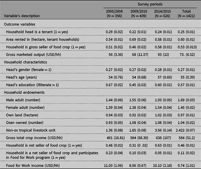
Source: Norwegian University of Life Sciences and Mekelle University household panel.
The data employed for this study are an unbalanced panel involving 356 households in 2005/2006, 439 households in 2009/2010, and 626 households in the 2014/2015 cropping season. This is due to attrition of some households and the inclusion of additional households in each of the subsequent survey rounds. For instance, the baseline survey was conducted in 1998/1999 with 400 households and only 330 households appeared in the 2005/2006 survey, while 70 households were attrite. But additional 26 new households were included in the 2005/2006 survey, and the total sample size was 356 households. In the 2009/2010 survey, only 294 households who participated in 2005/2006 appeared in the survey but 62 households were attrite, while additional 226 new households were included and the total sample of the 2009/2010 survey was 520 households. Similarly, in the 2014/2015 survey period, only 481 households involved in 2009/2010 appeared, while 39 households were attrite. But additional 151 new households were included and the total sample size becomes 632.Footnote 2 The death of the household head (if he/she lives alone), migration, and nonresponse of household heads were the reasons for attrition. A probit attrition model was used to assess and control the attrition bias by making use of the baseline data from 1998/1999. In the attrition model, households who drop out in each survey round were given the value 1, while available households were given the value of 0. Thus, the dependent attrition variable was constructed in this way and a probit regression of it is made on households’ and community-level variables that could determine attrition (for the detail, see Section 4.2).
The survey incorporated detailed questions on household features, land rental, and output market participation. The household features related questions asked about household head’s gender, age, literacy, marital status, and the amount of active labor force that the household has. Households’ output market participation survey includes questions on the types and quantities of agricultural products (staple food and cash crops) produced, consumed, and sold using community-level median price for valuation. Crop’s price varies across the survey periods and gives only the nominal value of marketed output. To get the real (inflation-adjusted) values over the three survey periods, first, I deflated the marketed output of each year by the 2009/2010 as a base year consumer price index. Then, the real value of marketed output sold in each year was changed to USD using the respective years exchange rate.Footnote 3 Finally, the household survey was supplemented by community-level information gathering that included one-way travel (walking) time to reach the nearby market place measured in hour, whether farm households are access to irrigation (yes = 1, 0 otherwise). Unlike to previous works that climate variables (rainfall) collected from the nearest weather station in developing countries like Ethiopia are set to cover wider geographical areas and thus their use as climate shock variables at micro-level is less meaningful, the current study uses daily satellite rainfall data captured at community level from the African Rainfall Climatology Version 2 (ARC2) precipitation estimates.
3.2 Descriptive analyses
Table 1 presents the summary statistics of some key household-level variables by survey period. On average, the percentage of tenant households who seek extra unit of land to adjust with their non-land resource endowment at least in one of the cropping season is 25%. The average area rented in by potential tenant households in the study region accounts for 0.60 hectare. I disaggregated households’ output market participation into gross and net sellers of crops (for both food and cash crops). This is to mean that a given household may sell a small amount and purchase a large amount of crops or vice versa. This categorization helps to assess whether a given household falls under a net buyer category or a net seller category in the output market. Accordingly, Table 1 shows that on average, the percentage of net seller households was smaller than that of gross seller households by 7%.
4. Model specification, attrition bias, and estimation strategy
4.1 Model specification
The conceptual framework is designed to estimate the impact of area rented in on participation and extent of participation in the output markets as a crop seller. Households’ market integration in selling crop output (Q s it ) is demonstrated as a two-stage decision. First, the household decides whether to participate as a seller of food or cash crops in the output market, and in the second stage, household decides on the amount of crop take to the market for sale. Thus, smallholder farmers’ decision on output market integration is modeled as a function of household characteristics, community-level factors, and unobservable individual heterogeneity effect. To show the causal impact, the households’ output market participation decision is specified as
 $${m_q}_{_{it}}\left| {Q_{it}^s = {\rm{}}{\rho _1}{{X'}_{it}} + {\rho _2}{R_{it}} + {C_i} + {\rho _3}{{D'}_{it}} + {\rho _4}{Y_t} + {\varepsilon _{it}}} \right|{\tau _{it}},$$
where mq
the likelihood of the households’ entry to the output market with a value of 1 for those who entered as crop sellers and 0 otherwise.
 $$Q_{it}^s{\rm{\;}}$$
is inflation-adjusted value of crop output sold in the product market (i.e., value of crop that is being commercialized).
$$Q_{it}^s{\rm{\;}}$$
is inflation-adjusted value of crop output sold in the product market (i.e., value of crop that is being commercialized).
 $$X'$$
is a vector of household-level control variables and includes(a) household head characteristics such as gender, age, and literacy status. The gender distribution of household heads helps to control on most market relating decisions. The human productive element of the household (farming experience proxy by head’s age) presents the ability to undertake farming with less difficult and literacy status of heads that apply their effort to exploit the land rental and output market opportunities. (b) The number of male and female adults in the household. Households with a higher number of active labor force are more likely to participate in the output market as crop sellers due to the importance of productive labor in efficient cultivation of the land and generating a possible surplus product for the market. (c) Land endowments of the household are expressed by certified landholding, while the non-land endowments are proxy by oxen ownership (number of oxen) and non-oxen live stocks [in tropical livestock unit] and other farm and non-farm assets. Households with a higher number of oxen are more likely to participate in the output market as a crop seller. This is due to the importance of oxen in cultivating additional unit of land (possibly obtained by renting in land) and enables to produce of surplus output. The non-land endowments may not be strictly exogenous variables. Therefore, I run models with and without these variables to check how susceptible result is to this possible endogeneity. Own landholding, however, is considered as an exogenous variable as it is less frequently adjusted over time in the study areas.
$$X'$$
is a vector of household-level control variables and includes(a) household head characteristics such as gender, age, and literacy status. The gender distribution of household heads helps to control on most market relating decisions. The human productive element of the household (farming experience proxy by head’s age) presents the ability to undertake farming with less difficult and literacy status of heads that apply their effort to exploit the land rental and output market opportunities. (b) The number of male and female adults in the household. Households with a higher number of active labor force are more likely to participate in the output market as crop sellers due to the importance of productive labor in efficient cultivation of the land and generating a possible surplus product for the market. (c) Land endowments of the household are expressed by certified landholding, while the non-land endowments are proxy by oxen ownership (number of oxen) and non-oxen live stocks [in tropical livestock unit] and other farm and non-farm assets. Households with a higher number of oxen are more likely to participate in the output market as a crop seller. This is due to the importance of oxen in cultivating additional unit of land (possibly obtained by renting in land) and enables to produce of surplus output. The non-land endowments may not be strictly exogenous variables. Therefore, I run models with and without these variables to check how susceptible result is to this possible endogeneity. Own landholding, however, is considered as an exogenous variable as it is less frequently adjusted over time in the study areas.
When controlling for the potentially endogenous endowment variables, I have included the deviations from the means and the means effect of all time-variant variables as the endowment effects themselves are of interest beyond being controls for endogeneity. While this is like using the Mundlak−Chamberlain device, it also allows us to assess the importance of resource endowment levels versus changes in them. The area rented in variable measured in hectare in equation (5) is an endogenous variable represented by
 $$\;R$$
, with the corresponding parameter
$$\;R$$
, with the corresponding parameter
 $$\;\rho .\;{c_\;}$$
is an unobservable heterogeneity effect, while
$$\;\rho .\;{c_\;}$$
is an unobservable heterogeneity effect, while
 $$\;D\;$$
is a vector of community-level variables, including distance to nearby market, rainfall, access to irrigation, and zone dummy.
$$\;D\;$$
is a vector of community-level variables, including distance to nearby market, rainfall, access to irrigation, and zone dummy.
 $${\varepsilon _.}\;$$
and
$${\varepsilon _.}\;$$
and
 $$\tau $$
are the error terms for the participation and intensity of participation in the output market models, respectively.
$$\tau $$
are the error terms for the participation and intensity of participation in the output market models, respectively.
 $$i$$
and
$$i$$
and
 $$t$$
are individual and time identifiers, respectively. A year dummy (
$$t$$
are individual and time identifiers, respectively. A year dummy (
 $${Y_t}$$
) is also included to control for change in smallholders’ output market integration in the 2009/2010 and 2014/2015 cropping seasons in reference to 2005/2006.
$${Y_t}$$
) is also included to control for change in smallholders’ output market integration in the 2009/2010 and 2014/2015 cropping seasons in reference to 2005/2006.
Equation (5) is estimated taking
 $${R_{it}}$$
as a censored variable with a positive value for households who participated in the land rental market as a tenant and zero otherwise. Since participation in the land rental market is affected by supply and demand factors, this variable is potentially endogenous. Thus, it becomes improper to use ordinary least square as it could lead to bias. Since the
$${R_{it}}$$
as a censored variable with a positive value for households who participated in the land rental market as a tenant and zero otherwise. Since participation in the land rental market is affected by supply and demand factors, this variable is potentially endogenous. Thus, it becomes improper to use ordinary least square as it could lead to bias. Since the
 $$cov\;\left( {{R_{it,}}{\varepsilon _{it}}} \right)\;\;$$
is different from zero in the output market models, definitely there are endogeneity issues. The mechanism of handling this endogeneity issues is discussed in the estimation strategy section.
$$cov\;\left( {{R_{it,}}{\varepsilon _{it}}} \right)\;\;$$
is different from zero in the output market models, definitely there are endogeneity issues. The mechanism of handling this endogeneity issues is discussed in the estimation strategy section.
Had the model in equation (5) been linear, the parameters could have been estimated using a fixed-effect (FE) model so that the unobservable heterogeneity effect could be removed through the demeaning process. However, FE model is appropriate for linear models and less likely applied for nonlinear models like what I did here. Applying the random effect, on the other hand, leaves the unobservable heterogeneity effect uncontrolled. In such a situation, the correlated random effect (CRE) or the Mundlak−Chamberlain approach is preferred as developed by Mundlak (Reference Mundlak1978) and Chamberlain (Reference Chamberlain1992). The merit of the CRE estimator is that it includes the mean value of all the time-varying variables into the regression analysis to control for the effect of time-invariant variables (Wooldridge, Reference Wooldridge2009). In the Mundlak−Chamberlain equation, the unobservable heterogeneity variable (
 $$C$$
) is expressed as a function of the average time-variant variables.
$$C$$
) is expressed as a function of the average time-variant variables.
 $${C_i} = \omega {\overline X_i} + {\mu _i},$$
where ${\overline X_i}$
is the mean value of time-varying variables (in the cross-sectional unit and it is the same for a given household over the survey periods while different between sampled households). μ is an error term with mean zero and constant variance and assumed uncorrelated with
${\overline X_i}$
(Wooldridge, Reference Wooldridge2010). Equation (6) is similar in spirit to the within transformation and produces the fixed effects slope estimator when used with a balanced panel data with,
${\overline X_i}$
is the mean value of time-varying variables (in the cross-sectional unit and it is the same for a given household over the survey periods while different between sampled households). μ is an error term with mean zero and constant variance and assumed uncorrelated with
${\overline X_i}$
(Wooldridge, Reference Wooldridge2010). Equation (6) is similar in spirit to the within transformation and produces the fixed effects slope estimator when used with a balanced panel data with, ${X_{it}} = {\overline X_i},T, \ldots ,N,$
… (Mundlak Reference Mundlak1978). However, the data used in this paper are unbalanced panel data. Hence, equation (6) is not equal to the usual within transformation. This is because it models
${X_{it}} = {\overline X_i},T, \ldots ,N,$
… (Mundlak Reference Mundlak1978). However, the data used in this paper are unbalanced panel data. Hence, equation (6) is not equal to the usual within transformation. This is because it models
 $${c_i}$$
as a function of
$${c_i}$$
as a function of
 $${\bar X_{i}} = {T^{ - 1}}\sum\nolimits_{t = 1}^T {{X_{it}}} $$
(that are not distorted by selection) (Semykina and Wooldridge, Reference Semykina and Wooldridge2010).
$${\bar X_{i}} = {T^{ - 1}}\sum\nolimits_{t = 1}^T {{X_{it}}} $$
(that are not distorted by selection) (Semykina and Wooldridge, Reference Semykina and Wooldridge2010).
Therefore, substituting equation (6) into equation (5) gives full Mundlak−Chamberlain equation provided that
 $${\mu _i} + {\varepsilon _{it = }}{U_{it}},$$
Footnote 4
$${\mu _i} + {\varepsilon _{it = }}{U_{it}},$$
Footnote 4
 $${m_q}_{it}\left| {Q_{it}^s = {\rm{}}{\rho _1}{{X'}_{it}} + {\rho _2}{R_{it}} + {\rho _3}{{D'}_{it}} + {\rho _4}{Y_t} + {\rho _5}{{\overline X}_i} + {U_{it}}} \right|{\zeta _{it}}.$$
Therefore, the likelihood of output market participation is estimated using a CRE probit model, while the extent of marketed output is estimated using a CRE tobit model.
 $${U_{it}}and{\zeta _{it}}$$
are the error terms for the probit and tobit models of equation (7), respectively.
$${U_{it}}and{\zeta _{it}}$$
are the error terms for the probit and tobit models of equation (7), respectively.
4.2 Attrition bias
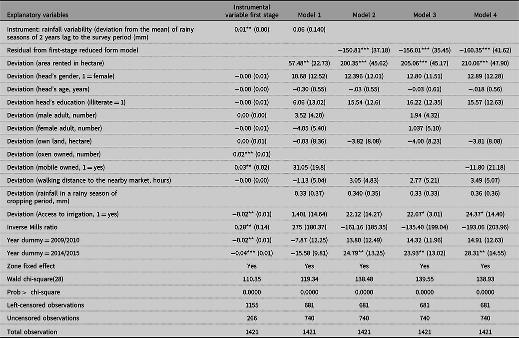
As mentioned earlier, there may also be attrition bias, and this problem is going to be taken care of using an attrition probit model, which is estimated using the baseline survey data of 1998/1999 and the subsequent survey rounds (i.e., 2005/2006, 2009/2010, and 2014/2015). The attrition probit estimation results are presented in Appendix Table A1, and results indicate that several of the explanatory variables are significant. This shows that attrition was nonrandom and there would have been a bias due to attrition. This potential bias is controlled for by including the Inverse Mills Ratio from the attrition regression as an additional regressor in the second-stage specifications.
4.3 Estimation strategy (endogeneity)
Access to rent in land is an endogenous variable and this needs to be taken into account when estimating its impact on output market participation and marketed output. The possible source of endogeneity could be unobservable individual heterogeneity. Providentially, this study uses panel data, which can ease the process of controlling the endogeneity problem. This implies that the unobservable individual heterogeneity effect is time-invariant within the household so that the Mundlak−Chamberlain specification removes the unobservable heterogeneity effect from the land rental and output market participation models (Wooldridge, Reference Wooldridge1995). Nonetheless, still, there is a possibility that area rented in could be an endogenous regressor in the outcome equation (6) due to potential correlation with leftover household and community-level unobservable time-varying heterogeneity.
The possible way of solving the endogeneity sourced from unobservable time-varying heterogeneity is using the instrumental variable (IV) method. Alternatively, for a linearly endogenous regressor, a control function approach relies on the alike kinds of identification conditions (Wooldridge, Reference Wooldridge2009, Reference Wooldridge2010). More specifically, equation (5) is specified separately into area rented in variable that is censored at zero in the first stage, equation (8), and market integration in the second stage, equation (9),Footnote 5 respectively as follows:
 $${R_{it}} = {\gamma _1}Z{{\rm{'}}_{it}} + {\gamma _2}X{{\rm{'}}_{it}} + {\gamma _3}D{{\rm{'}}_{it}} + {\gamma _4}{\overline X_\iota } + {\gamma _5}{Y_t} + {c_i} + {\xi _{it.}}$$
 $${m_q}_{it}\left| {Q_{it}^s = {\rm{}}{\rho _1}{{X'}_{it}} + {\rho _2}{R_{it}} + {\rho _2}\widehat {{\xi _{\iota t.}}} + {\rho _3}{{D'}_{it}} + {\rho _4}{Y_t} + {\rho _5}{{\overline X}_\iota } + {c_i} + {U_{it}}} \right|{\zeta _{it}}.$$
The control function approach requires exclusion restriction variables (
 $$Z{'_{it}})$$
in the reduced form equation (8). These have to be uncorrelated with the error term in equation (9),
$$Z{'_{it}})$$
in the reduced form equation (8). These have to be uncorrelated with the error term in equation (9),
 $${\rm{c}}ov\left( {{{Z'}_{it}},{U_{it}}|{\zeta _{it}}} \right) = 0$$
, and correlated with the endogenous variable
$${\rm{c}}ov\left( {{{Z'}_{it}},{U_{it}}|{\zeta _{it}}} \right) = 0$$
, and correlated with the endogenous variable
 $$cov\left( {{R_{it}},{{Z'}_{it}}} \right) \ne 0.$$
The error term generated from the random effect tobit model
$$cov\left( {{R_{it}},{{Z'}_{it}}} \right) \ne 0.$$
The error term generated from the random effect tobit model $\widehat {({\xi _{\iota t.}})}$
is then included as a regressor in equation (9). The statistical significance of the residual provides a test for endogeneity of the area rented in variable. As in a two-stage IV model, the control function approach requires exclusion restrictions as discussed above. In this case, rainfall variability (deviation from the mean) of the rainy season of 2 years lag to the survey period was used as an instrument.
Footnote 6,Footnote 7
The intuition is that production risk could be one of the important reasons for a preference for sharecropping contracts particularly by tenants who may be willing to pay only very low fixed rents as an alternative contract when production risk is high, thereby making sharecropping optimal for both parties. In this case, rainfall variability in 2 years lag rainy season to the survey period leads to increase landlords’ participation in the rental market after such shock. This is because, after shocks, landlords may have to rent out more land in sharecropping (the dominant land rental contract arrangement in the study region) as they prefer to share the production risk and reduced the risk of buying food crops in the next period as reported by Gebregziabher and Holden (Reference Gebregziabher and Holden2011). This may thus enhance tenant’s access to land through renting in the year after such shocks. I test the statistical validity of this by including the instrument in the output market participation equations in one specification. If the instrument was insignificant in the output market models but significant in the area rented in model, and if the error term from the first-stage model (the difference between the observed and predicted areas rented in) was significant in the output market models, then, endogeneity is an issue and was corrected for with the control function.
$\widehat {({\xi _{\iota t.}})}$
is then included as a regressor in equation (9). The statistical significance of the residual provides a test for endogeneity of the area rented in variable. As in a two-stage IV model, the control function approach requires exclusion restrictions as discussed above. In this case, rainfall variability (deviation from the mean) of the rainy season of 2 years lag to the survey period was used as an instrument.
Footnote 6,Footnote 7
The intuition is that production risk could be one of the important reasons for a preference for sharecropping contracts particularly by tenants who may be willing to pay only very low fixed rents as an alternative contract when production risk is high, thereby making sharecropping optimal for both parties. In this case, rainfall variability in 2 years lag rainy season to the survey period leads to increase landlords’ participation in the rental market after such shock. This is because, after shocks, landlords may have to rent out more land in sharecropping (the dominant land rental contract arrangement in the study region) as they prefer to share the production risk and reduced the risk of buying food crops in the next period as reported by Gebregziabher and Holden (Reference Gebregziabher and Holden2011). This may thus enhance tenant’s access to land through renting in the year after such shocks. I test the statistical validity of this by including the instrument in the output market participation equations in one specification. If the instrument was insignificant in the output market models but significant in the area rented in model, and if the error term from the first-stage model (the difference between the observed and predicted areas rented in) was significant in the output market models, then, endogeneity is an issue and was corrected for with the control function.
5. Results and discussions
5.1 Impacts of area rented in on smallholders’ commercialization
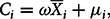
Table 2 provides the estimation results regarding factors that affect the probability of smallholder farmers’ output market participation as a crop seller. Regression results are presented in marginal effects as coefficients of marginal effects are more informative in nonlinear models. The second column in Table 2 is the first-stage IV model of area rented in estimated using CRE tobit model. As shown, the rainfall variability of rainy seasons of 2 years lag to the survey period was significant at the 1% level and has a positive sign. This indicates that weather shock has lagged positive effect on the extent of land rental market participation from the tenant side. As presented, the instrument is significant in the first-stage model (Model 1) at the 1% level while it is insignificant in the second-stage model (Model 2). Table 2 also includes the residuals from the first-stage reduced form equation along with the observed area rented in variable. The inclusion of the residual term tests and controls for the endogeneity of area rented in the output market models. The residual is significant at the 1% level with a negative sign in all second-stage models. Therefore, the control function approach appears to have worked properly.
Table 2. The impact of area rented in on smallholders’ commercialization (correlated random effect probit): (area rented in is treated as endogenous). Marginal effect after xtprobit
Notes: MC probit models using the mean (not reported) and deviation from the mean of time-variant variables. *: 10%, **: 5%, ***: 1%, refers to the level of significance. Numbers in parenthesis are robust standard errors.
Source: NMBU and MU household panel survey.
Four different specifications of the second-stage model are used to estimate the probability of output market participation in the output market as a crop seller by tenant households (see Table 2). Model 1 included the instrument as a test for its statistical validity, while Model 2 excluded the instrument but included the strict exogenous variables in their mean and deviation from the mean. Model 3 included the non-strict exogenous household labor endowment (adult male and adult female) variables in their deviation from the mean and mean value as a Mundlak−Chamberlain device. Model 4 included other household endowment variables such as mobile phone ownership. Alternative model specifications are used to assess the robustness of the results to the inclusion of potentially endogenous endowment variables that may improve the likelihood of participation in the output market.
The area rented in variable is found to have a significant effect with a positive sign on the likelihood of output market participation in all second-stage models (see Table 2). This supports the prior expectation that access to an extra unit of land by a tenant increases the probability of output market participation as a crop seller. The marginal effect shows that, on average, 1 hectare increase in the area rented in by tenant households leads to an increase in the probability of participation in the output market as a crop seller by about 60% (Model 2), ceteris paribus. This result is much higher than the likelihood of output market participation for equal changes in own land (see Table 2) and provides compelling evidence in support of land rental market positively affecting smallholder farmers’ commercialization.
Part of the reason to include other control variables in the models was to see whether variables other than area rented in influence smallholder farmers’ commercialization. To this end, I consider whether household head’s characteristics such as age, gender, and literacy status make a visible impact on the likelihood of output market participation. The findings indicate insignificant impact of head’s age, head’s gender, and head’s literacy status in the sample. I also assessed whether smallholder farmers’ output market participation has changed over the survey periods. The results show that the likelihood of smallholder farmers’ output market participation as a crop seller improved in the year 2014/2015 compared to 2005/2006 by about 18% (Model 2). The possible justification could be first, as a result of substantial public investment in irrigation, especially during the Growth and Transformation Plan Phase 1 (GTP-1) launched from 2010/2011 to 2014/2015, smallholders from the study region are accessible to irrigation and enable to harvest more than once per year and cultivate cash crops. Second, the development of infrastructure such as access to road, market, and transport service significantly reduces the transaction costs and enhanced smallholders’ market integration over time. Third, the recently established farmers’ union and cooperatives provide updated and better market information about the type of products to be produced, the right product price, the right customer, and market place and improved the bargaining power of smallholders over traders and customers. Fourth, the expansion of agricultural products supermarkets (vegetables, fruits, and grass-root crops) in urban areas boosts to the production of cash crops and improves the value chain system of the sector in various aspects, such as access to products market, extension services, and agro-processing activities.
Table 2 shows that access to irrigation has a strong effect with a positive sign on farmers’ output market integration. The marginal effect shows that, on average, access to irrigation increases the probability of output market participation of farm households as crop sellers by 12–13%, ceteris paribus. The result is consistent with the finding of Gebregziabher, Namara, and Holden (Reference Gebregziabher, Namara and Holden2009), which showed that irrigated farm households greatly participated in the output market compared to rainfed farm households in the same study region.
5.2 The impact of area rented in on marketed output
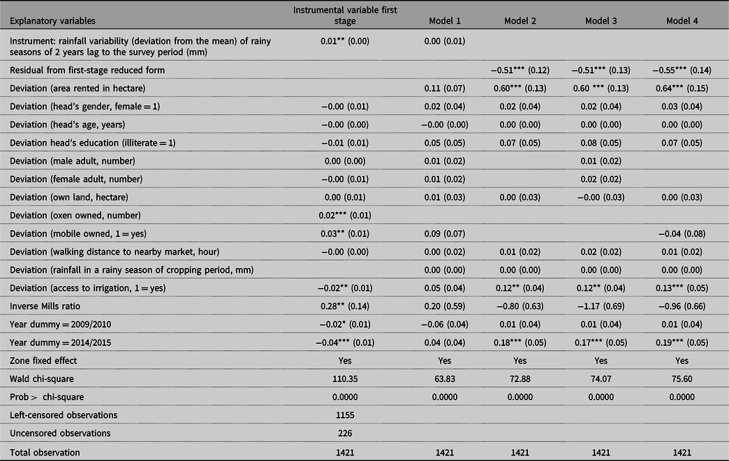
The results for the impact of area rented in on the extent of participation in the output market by smallholder farmers are presented in Table 3. These models also assess the extent of strictly exogenous variables and also control for individual unobserved heterogeneity effect using the Mundlak−Chamberlain technique. Estimating the impact of area rented in on the marketed output is also demonstrated as the first- and second-stage specifications in the same fashion to the probability of participation. Results show that the instrument variable is insignificant in the second-stage models while significant in the first IV stage.
Table 3. The impact of area rented in on the amount of marketed output (correlated random effect tobit): (area rented in is treated as endogenous).Marginal effect after xttobit
Notes: MC tobit models using the mean (not reported) and deviation from the mean of time-variant variables. *: 10%. **: 5%. ***: 1% refers to the level of significance. Numbers in parenthesis are standard errors bootstrapped at households with 400 replications.
Source: NMBU and MU household panel survey.
The area rented in variable has a strong positive effect on the intensity of smallholder farmers’ output market participation in three of the second-stage models at the 1% level. Exclusion of the endowment variables (adult male, adult female, and mobile ownership) from the second-stage estimation slightly reduces the coefficient of area rented in. This may indicate that the endowment variables adjust themselves over time and could possibly be endogenous variables. On average, the marginal effect results show that the change of area rented in by 1 hectare leads to an increase in the marketed output sold in the market by smallholder farmers from US$ 200 to US$ 210 per household per year. These results show to some extent that land rental market has facilitation power in smallholders’ agricultural commercialization.
Results from Table 3 also revealed that farm household endowments such as ownership of communication devices (i.e., mobile phone) have a positive but insignificant effect on the extent of output market participation by smallholder farmers in any of the models. The intuition was that farm households with mobile phone ownership are expected to enhance market integration of smallholder farmers by enabling them to acquire better market information thereby reducing fixed transaction costs, but show insignificant results. Access to irrigation is another variable found to have a strong and positive effect on smallholders’ level of commercialization. This might happen as irrigation reduces production risk and creates suitable situation for the cultivation of cash crops. The marginal effect shows that farm households with access to irrigation had increased their marketed output by about US$ 22–23/year compared to nonirrigated farm households at the 10% level. Even though adequate rainfall during the production season was supposed to increase total production and could contribute to higher crop selling, the results show that it does not. This may indicate that if smallholders’ commercialization is expanded with the expansion of irrigation, not dependence on rainfall, is the way to do it.
6. Conclusion and policy implication
This study employed the theory of tenant’s access to land and output market participation under imperfect input and output markets and transaction costs. Based on this theory and a panel data of rural farm households collected in 2005/2006, 2009/2010, and 2014/2015 cropping seasons in Tigrai, northern Ethiopia, this study assesses the effect of tenant’s access to land renting on participation in the product market as crop sellers and the amount of marketed output that they sell. The study employed the Mundlak−Chamberlain approach to fix the problem of individual unobservable heterogeneity effect with alternative model specifications to assess the robustness of the findings. Results showed that coefficients are fairly stable among the different specifications. Endogeneity issues with regard to land renting in were handled using the control function approach with 2 years lag to the survey period rainfall variability (deviation from the mean) serving as an instrument variable. The result showed that this variable is a significant determinant of area renting in but not smallholder farmers’ commercialization.
This study found that the extent of land rented in has a significant effect on both participation and the size of output sold in the product market (commercialization). This is happening despite the prevalence of imperfect input markets and high transaction cost of entry to land rental market in the study region (Holden and Ghebru, Reference Holden and Ghebru2013, Reference Holden and Ghebru2016), this result indicates that the current land rental market in Ethiopia to some extent contributes positively to rural transformation through more market-oriented production. This indicates the importance of having a mechanism that could enhance the transfer of land from an inefficient farmer to more efficient and progressive farmers even from smallholder farmers’ commercialization.
From a policy perspective, this study strengthens the existing knowledge in two points: first, promoting land rental markets is an important strategy to improve smallholder farmers’ commercialization in a land-scarce economy through land use right transfer from unproductive and inefficient farmer to productive, efficient, and an entrepreneurial farmer. Enhancing the tenure security of landholders through the implementation of the land registration and certification program facilitates this land rental transaction among smallholders. This may also provide an important pathway in attaining economic transformation through agricultural growth in which the Ethiopia government aims to do. Hence, it is necessary to design policies and strategies with a view to enhance the level of smallholders’ commercialization by means of land renting that provides room for more production for the market.
Second, there is a considerable and growing body of literature that suggests irrigation development serves as a vehicle of higher crop production, poverty reduction, and overall welfare improvement of farm households. The Ethiopian government in general and the regional government of Tigrai, in particular, consider that small-scale irrigation is a key and potential strategy to supplement rainfed agriculture and improve agricultural production and reduce rural poverty. In view of that, the regional government of Tigrai introduced an ambitious irrigation development plan, especially in the region’s GTP-1 that has been launched from 2010/2011 to 2014/2015. When looking at the practice of irrigated agriculture, from the total arable land of the region, area planted with irrigation has been increased from 9% in 2010/2011 to 15% in the 2013/2014 cropping period. This may affect smallholders’ commercialization in three ways: (a) irrigation potentially encourages to produce more than once per year and increased plot-level productivity. Then, farmers enable to produce surplus products, perhaps beyond home consumption and expected to improve the amount of crops sold in the market. On the mean time, irrigation enhances the production of high value or cash crops and improves smallholders’ market integration; (b) irrigation creates crowding-in effect on adoption of modern agricultural technologies such as inorganic fertilizer. More specifically, farmers prefer to use fertilizer in irrigated plots to rainfed plots as irrigation is a complementary input to inorganic fertilizer. Such practice increases plot-level productivity and potentially generates a surplus product that will be exported to the market for sale; and (c) irrigation also affects smallholders’ commercialization through land rental market. The intuition is that irrigation reduces production risk and potential and entrepreneurial farmers motivate to rent in extra area of irrigated plots to scale up their production and gradually shift the farming system from subsistence to market-oriented. Therefore, public investment in small-scale irrigation in the study region substantially drives to change the structure of land rental market and the value chain system of agricultural products and facilitates the rural transformation.
Acknowledgments
The author acknowledges to the Relief Society of Tigrai (REST) for providing satellite rainfall data for the study sites.
Financial support
Data collection has been funded by NORAD through the NOMA and NORHED programs, especially the “Climate-Smart Natural Resource Management and Policy” collaborative research and capacity-building program between the School of Economics and Business in Norwegian University of Life Sciences, the Department of Economics in Mekelle University, Ethiopia, and the Department of Agricultural Economics (LUANAR) in Malawi.
Conflict of interest
None.
Table A1. Probit estimation of attrition based on the baseline sample of 1998/1999
Notes: *, **, and *** represent 10%, 5%, and 1% level of significance, respectively. Numbers in parenthesis are robust standard errors.
Source: NMBU and MU household panel.


 Open access