


INTRODUCTION
The Greenland ice sheet discharges over 1000 Gt of freshwater to the oceans annually (Bamber and others, Reference Bamber, Van Den Broeke, Ettema, Lenaerts and Rignot2012); a rate that exceeded the annual accumulation of snow and ice by 378 Gt a−1 between 2009 and 2012 (Enderlin and others, Reference Enderlin2014). Freshwater flux takes the form of both liquid freshwater discharge and solid ice calved from tidewater glaciers, with the latter making up 32–50% of the total (van den Broeke and others, Reference van den Broeke2009; Enderlin and others, Reference Enderlin2014). Discharge of both solid and liquid freshwater increased at a rate of 25.4 Gt a−2 from 2003 to 2013 (Velicogna and others, Reference Velicogna, Sutterley and Van Den Broeke2014). Increases in freshwater discharge can decrease surface water salinity both locally in waters within fjords and on the continental shelf and more broadly throughout the North Atlantic, potentially affecting the Atlantic Meridional Overturning Circulation (Fichefet and others, Reference Fichefet2003; Stouffer and others, Reference Stouffer2006; Yang and others, Reference Yang2016). Thus, accurate observations of iceberg geometries (e.g., volumes, keel depths, waterline length) and their distributions in time and space are necessary to estimate their impact on seawater properties and for the initiation and validation of ocean circulation models that include thermodynamically active icebergs (e.g., Stern and others, Reference Stern, Adcroft and Sergienko2016).
Around Antarctica, iceberg size distributions have been described for limited numbers of medium to large (>100 m length) icebergs observed using radar and sextant (Wadhams, Reference Wadhams1988) or by direct visual observation (Neshyba, Reference Neshyba1980). Satellite data have been used to describe iceberg distributions throughout the Southern Ocean, though these observations are also restricted to lengths >100 m (Neshyba, Reference Neshyba1980; Tournadre and others, Reference Tournadre, Girard-Ardhuin and Legrésy2012; Tournadre and others, Reference Tournadre, Bouhier, Girard-Ardhuin and Rémy2016). These observations are informative but they are not directly analogous to iceberg distributions in Greenland fjords as they focus primarily on large, tabular icebergs in open ocean areas rather than in constricted fjords.
Observations of icebergs in the Arctic are scarce with distributions and dimensions of only a limited number (n < 600 within each study) of icebergs, bergy bits and growlers as described (Hotzel and Miller, Reference Hotzel and Miller1983; Smith and Donaldson, Reference Smith and Donaldson1987; Dowdeswell and Forsberg, Reference Dowdeswell and Forsberg1992; Crocker, Reference Crocker1993). Iceberg draughts were detected for 285 icebergs in Sermilik Fjord using an inverted echo sounder (Andres and others, Reference Andres, Silvano, Straneo and Watts2015), and sonar profiles of iceberg keels were obtained for nine icebergs near Labrador (Smith and Donaldson, Reference Smith and Donaldson1987). Using stereo satellite imagery Enderlin and Hamilton (Reference Enderlin and Hamilton2014) calculated iceberg volumes and melt rates, and estimated iceberg keel depths and Enderlin and others (Reference Enderlin, Hamilton, Straneo and Sutherland2016) found melt rates and calculated the freshwater flux of icebergs in ice mélange. Iceberg movements, important for determining residence times of icebergs in fjords, location of freshwater input and identifying broad circulation patterns, have been tracked with GPS transmitters (Sutherland and others, Reference Sutherland2014a; Larsen and others, Reference Larsen, Overgaard Hansen, Buus-hinkler, Krane and Sønderskov2015). Critically, there are no fjord-wide descriptions of iceberg distributions or investigations into the influence of glacier depth and calving style on iceberg properties.
Here, we use multiple satellite datasets to quantify and compare iceberg characteristics over larger spatial scales, for larger populations of icebergs (n > 105) and with finer resolution of size (~30 m) than has previously been achieved. We compare iceberg characteristics across three distinct fjords in Greenland and quantitatively assess the size-frequency distribution of icebergs and how they vary both along-fjord and in time. Our results provide statistically significant fits to iceberg size distributions and information on keel depths that allow a baseline estimate of total iceberg melt in these three Greenland fjords.
Physical setting
We examine three glacial fjord systems in two regions of Greenland: Sermilik Fjord (SF) in the southeast; and Rink Isbræ Fjord (RI) (also known as Karrats Isfjord) and Kangerlussuup Sermia Fjord (KS) on the west coast, both within the greater Uummannaq Bay (Fig. 1). These three fjords were chosen based on the availability of hydrographic data, tracked icebergs via GPS (e.g., Sutherland and others, Reference Sutherland2014a), and the diverse range of calving styles and grounding line depths of the glacier termini. Additional physical features of each fjord are identified in Figure S2.

Fig. 1. (a, inset) The location of the three study fjords Rink Isbrae (RI), Kangerlussuup Sermia (KS) and Sermilik Fjord (SF). (a) RI and KS are shown in a Landsat 8 image from 7/8/14, and (b) SF is shown in a Landsat 8 image from 7 August 2014 (NASA Landsat Program, 2014). Distances (km) from glacial termini are shown along colored lines in both panels, along with depths of major sills into each fjord.
Sermilik Fjord (SF)
SF is the outlet to the Irminger Sea for icebergs calved from Helheim Glacier (Fig. 1), as well as the smaller Fenris and Midgaard glaciers. Reaching speeds of 8–11 km a−1 along its trunk, Helheim Glacier is one of Greenland's most prolific iceberg producers (~25 Gt a−1) (Moon and others, Reference Moon, Joughin, Smith and Howat2012; Enderlin and others, Reference Enderlin and Hamilton2014). The northern portion of the ~600 m deep, ~5.5 km wide terminus is periodically at flotation, while the southern portion is grounded (Murray and others, Reference Murray2015). Ice calved from Helheim Glacier travels ~20 km to the east, often in a densely packed ice mélange, before extending to the south for ~80 km to the fjord mouth and the Irminger Sea. SF ranges from 8 to 12 km wide and 600–900 m in depth, and lacks a shallow sill at its mouth (Sutherland and others, Reference Sutherland2013). During summer, the fjord generally contains a layer of relatively cold (~0.5°C) and fresh Polar Water to depths in a range 100–200 m, above a layer of warmer (up to 4°C), saltier Atlantic Water (Sutherland and others, Reference Sutherland, Straneo and Pickart2014b). SF has been the subject of many investigations on circulation and hydrography (Straneo and others, Reference Straneo2010; Sutherland and others, Reference Sutherland, Straneo and Pickart2014b), calving dynamics (Murray and others, Reference Murray2015) and iceberg motion (Sutherland and others, Reference Sutherland2014a), melting (Enderlin and Hamilton, Reference Enderlin and Hamilton2014) and keel depth (Andres and others, Reference Andres, Silvano, Straneo and Watts2015). Hereafter, we will refer to the entire system between Helheim Glacier and the Irminger Sea as SF.
Rink Isbræ Fjord (RI)
RI is the fjord into which Rink Isbræ (glacier) terminates (Fig. 1). The average speed is ~4.2 km a−1 near its 4.7 km wide terminus. The glacier is partially floating, reaching a depth of 840 m in water deeper than 1000 m (Bartholomaus and others, Reference Bartholomaus2016; Rignot and others, Reference Rignot2016). The fjord is 6–12 km wide and 1100 m deep along much of its length, running primarily east to west for ~65 km to its mouth in Uummannaq Bay. Karrats Island splits the end of the fjord into north and south arms at ~50 km down-fjord. On the southeast side of the island is a sill with a depth of 400 m, while on the island's north side a sill rises to ~230 m below the surface. RI contains cold (~1°C) fresh water to depths of 100–200 m overlaying warmer AW with temperatures up to 3°C in summer (Bartholomaus and others, Reference Bartholomaus2016).
Kangerlussuup Sermia Fjord (KS)
KS is the next fjord containing a marine-terminating glacier to the south of RI (Fig. 1). Despite its close proximity, KS has significantly different properties than RI. The glacier moves more slowly (~1.8 km a−1) than the glacier feeding RI, and is only 4.2 km wide and 250 m deep at its grounded terminus (Bartholomaus and others, Reference Bartholomaus2016; Rignot and others, Reference Rignot2016). The KS fjord runs generally east to west for ~63 km before opening to Uummannaq Bay. At 37 km down-fjord the fjord splits into north and south arms. KS is much shallower than RI, reaching depths of only ~500 m. At the mouth of the north arm there is a sill at a depth of 430 m, and another sill rises to 290 m depth on the near-glacier end of the south arm. Waters in KS are generally colder than those at corresponding depths within RI, with waters near 0°C to 100 m depth overlying waters up to 2°C in summer (Bartholomaus and others, Reference Bartholomaus2016).
METHODS
Overview
Using optical satellite imagery and position records from GPS units mounted on large icebergs, we examine and compare total ice (including icebergs, bergy bits, growlers and sea ice) coverage, individual and total iceberg volume and iceberg size distributions within and between the SF, RI and KS systems. We calculate iceberg areas using Landsat 8 (L8) images, and we use high-resolution DEMs to calibrate an iceberg area to volume relationship. Additionally, we assume idealized iceberg shapes and calculate upper and lower bounds on iceberg keel depths.
Landsat 8 image processing
We collected all cloud-free L8 images of SF, RI, and KS captured between 2013 and 2015 (Table 1). Images in which fjords contained substantial sea ice (i.e., images from before 1 July in SF and before 15 July in RI and KS each season) were not used. We used the panchromatic band (band 8) in each scene to take advantage of its higher spatial resolution (15 m) compared with the multispectral bands (30 m). Icebergs were delineated and measured using tools available in ArcMap and Orfeo Toolbox (OTB). Briefly, we defined pixels containing ice as those having a brightness above a threshold and found the total area of coverage of all types of ice for each image. We then combined adjoining ice pixels into polygons. Those polygons that contained multiple icebergs were split into individual icebergs either by hand or using a structural feature set (SFS) texture analysis technique where icebergs and iceberg edges stand out as irregular from background ice mélange. Details regarding each step of the iceberg identification and delineation are presented below.
Table 1. Total ice coverage and total area and volume of classified icebergs for each analyzed image
Total ice area
All ice was first delineated using a thresholding technique. L8 image data are distributed as scaled digital numbers (DN), which vary between images depending on the sun elevation angle (SE) at the image acquisition time (Fig. 2a). To standardize the threshold across all images, we converted a representative set of images from DN to values of top of atmosphere (ToA) reflectance (USGS, 2016). By inspecting the ToA reflectance values of ~50 pixels that were evenly split between water and ice, we determined that a reflectance of 0.28 W m−2 robustly separated pixels containing ice from those containing water (Figs 2b, c). For all images, we then found the DN value corresponding to a ToA reflectance value of 0.28 W m−2 using the formula
 $${\rm DN =} \displaystyle{{\sin} {\rm (SE) \times 0.28 - {\rm RAV}} \over {{\rm RMV}}}$$
where RAV is the ‘reflectance add value’, and RMV is the ‘reflectance multiplication value’ (USGS, 2016), which are recorded within the L8 metadata. Pixels with values higher than the threshold DN were defined as ice. Adjoining ice pixels were converted into polygons, and their areas were calculated (Fig. 2). We summed the areas of all ice polygons to calculate the total fjord area covered in ice for each image. To compare ice coverage and iceberg properties within fjords, we split fjords into bins of roughly equal distance from the termini and found the area of ice coverage within each bin. Mean lengths of bins are 3 km in SF and RI and 5 km in KS.

Fig. 2. The iceberg classification process. (a): Band 8 of an L8 image from 15 September 2014 containing SF is shown with the extents of panels (b) and (c) outlined in yellow, and (d) and (e) outlined in blue. (b): Individual icebergs are surrounded by open water throughout much of the fjord. (c): Pixels with a DN above an equivalent TOA reflectance of 0.28 W m−2 (DN > 11 412 in this image), shown in red, are delineated in iceberg polygons. (d): Areas with ice mélange (upper half) are smoothed using a boosted-mean filter (lower half). (e): The ‘length’ output of an SFS extraction run on the filtered image is shown in black and white. Pixels with low SFS-Length values (darker pixels) are defined as belonging to icebergs with minimum bounding convex hull polygons (red outlines) shown.
Individual iceberg separation and classification
In order to avoid multiple adjacent icebergs being counted as a single iceberg, we split polygons containing multiple icebergs into individual icebergs using two different methods. Iceberg boundaries are visible in L8 images as linear regions that are slightly lighter or darker than their surroundings (Fig. 2). We visually inspected all polygons created by the above thresholding method with areas >2 × 10⁴ m2. Those polygons containing multiple icebergs were then either split into individual iceberg polygons manually if the number of icebergs contained was small (<~20) or the data was clipped and exported to a new raster file for automated analysis. Single pixels that were above the threshold but not adjacent to any other pixels that were also above the threshold were removed. Many of those single pixels would only be partially filled with ice, and identifying them all as icebergs with a length of 15 m could overestimate the total ice volume (Table 1). Minimum areas of classified icebergs were bounded by the area of a simplified polygon incorporating two L8 pixels (450 m2).
To delineate icebergs in an ice mélange via the automated approach, we first applied a boosted mean filter to the raster datasets containing the ice mélange to minimize noise in images while retaining iceberg edges (Fig. 2d) (Williams and Macdonald, Reference Williams and Macdonald1995). The filter is made up of two steps: first, a 3 × 3 low-pass filter in which each pixel is assigned a new value equal to the average of itself and the 8 pixels with which it shares vertices is applied. For the second step the result of the low pass filter is then averaged with the original image.
We used the structural feature set (SFS) tool available in Orfeo Toolbox OTB (Huang and others, Reference Huang, Zhang and Li2007) on the result of the boosted mean filter (Fig. 2). The SFS tool compares the similarity of pixels to their surroundings. For each pixel in the dataset, the spectral difference and spatial distance between the central pixel and the next nearest pixel along equally spaced direction lines is determined. The line is extended if those values do not exceed user defined thresholds. We were unable to use standardized threshold values because of differences in DN ranges, lighting, shadows, and ice mélange surface between images. Instead, we compared the first band (SFS-length: the maximum length of direction lines) of multiple SFS output images using 20 directional lines and varying the spectral (2500–5000 DN) and spatial (12–50 pixel) thresholds. We determined which threshold combination best separated individual icebergs from the ice mélange for each image using these SF-length values. Icebergs and especially iceberg edges, generally displayed less uniformity than the surrounding mélange, resulting in low values of SFS-length (Fig. 2). We assigned SFS-length thresholds for each image by visually inspecting each image, then used the threshold to distinguish icebergs from the mélange. We combined adjoining iceberg pixels into polygons and calculated their areas. As above, we inspected all icebergs with an area >2 × 10⁴ m2 and manually split polygons containing multiple icebergs. We then replaced iceberg polygons with the minimum bounding convex hull that contained all iceberg pixels in order to fill holes and connect unclosed outer boundaries (Fig. 2e).
We examined the uncertainty of using the SFS tool to delineate icebergs by comparing the results to a manual classification method. We visually inspected a 16 km2 region of ice mélange in each of 5 L8 images and manually delineated all icebergs. We compared total ice area and iceberg size distribution of the two methods. Small icebergs and many edges of icebergs often cannot easily be seen in L8 images. Therefore, we also inspected and delineated by hand icebergs that could be seen within a 5.4 km2 region of ice mélange from a very-high resolution (0.5 m) Worldview image from 7 June 2016.
Non-iceberg ice correction
The thresholding technique used to define ice in L8 images does not differentiate between icebergs and sea ice, ice rafts, or small pieces of ice (bergy bits and brash ice), and the resolution of L8 images is insufficient to visually differentiate these ice types. Therefore, to calculate correction factors, we quantified the average iceberg portion of the total ice found using the thresholding technique in very-high resolution (~0.5 m) Worldview imagery. In SF we analyzed a 3 km2 region where ice concentrations were high near the ice mélange (images from 21 August 2011 and 29 June 2012) and a 12 km2 region where ice concentrations were lower in the open fjord (images from 15 July 2010, 11 July 2013, 30 July 2013, 15 August 2012 and 8 June 2015). In RI we analyzed a 16 km2 region in images from 25 June 2013, 4 July 2013, 17 July 2013, 11 August 2013 and 19 July 2014, and in KS we analyzed an 18 km2 region in images from 25 June 2013, 4 July 2013 and 17 July 2013. We used a thresholding technique as described above to delineate ice polygons, then visually inspected each ice polygon to determine if it was or was not an iceberg.
In SF, sea ice made up 42% of the total calculated volume of ice (we describe how we obtain ice volume from images of ice area below) in the image that we analyzed from 8 June 2015. In all other images sea ice made up an average of 3.31% (ranging 0.39–9.12%) of the total calculated volume of ice. We therefore removed L8 images acquired before July of each year. In images after 1 July, we use the sea-ice percentages calculated from Worldview images to correct the overestimation of icebergs in L8 images by removing a random sample of delineated icebergs from each of four size classes using the correction factors calculated from Worldview. We removed 7.9% of icebergs between 0 and 105 m3, 7.8% of icebergs between 105 and 2 × 10⁵ m3, 3.6% of icebergs between 3 × 10⁵ and 4 × 10⁵ m3, and 4.1% of icebergs with volumes >3 × 10⁵ m3.
In RI, sea ice made up 33% and 12% of the total calculated volume of ice in the images that we analyzed from 25 June 2013 and 4 July 2013, respectively, but only 2.3% in images after 15 July. We therefore exclude L8 images acquired before 15 July of each year, and removed a portion of delineated icebergs in L8 images acquired after 15 July equivalent to the proportion of non-iceberg ice present in Worldview imagery. Because total ice amounts were lower in RI than in SF we identified sea-ice amounts in two rather than four size classes. We removed 7.4% of icebergs between 0 and 3 × 10⁵ m3 and 4.6% of icebergs with volumes >3 × 10⁵ m3. We removed the same proportion of icebergs in L8 images from KS as total ice amounts were too low to derive independent correction factors there.
Area/volume relationships
We constructed DEMs of icebergs in SF to establish a relationship between iceberg area and volume. Eight DEMs were generated using very high resolution (~0.5 m) stereo imagery from the Worldview 1–3 satellites. We created DEMs using either the NASA Ames Stereo Pipeline (ASP) (Moratto and others, Reference Moratto, Broxton, Beyer, Lundy and Husmann2010) or the Surface Extraction with TIN-based Search-space Minimization (SETSM) (Noh and Howat, Reference Noh and Howat2015) algorithms (Table S1). Comparisons between DEMs generated by the two algorithms revealed random, non-systematic differences, justifying the merger of the two DEM datasets. All DEMs have a horizontal resolution of ~2 m and random errors of 3 m (Enderlin and Hamilton, Reference Enderlin and Hamilton2014).
For each DEM, we manually created polygon boundaries around icebergs. We then found the area and average elevation of each polygon. We calculated the elevation of the ocean surface by taking the average elevation of at least ten ice-free pixels dispersed throughout each DEM, and subtracted that elevation from the mean elevation of pixels making up each iceberg. We multiplied that mean elevation with the visible area of each iceberg to find its above water volume. Assuming an iceberg density of 920 kg m−3 and a fjord-water density of 1025 kg m−3, we calculated the underwater volume and total volume of each iceberg (Fig. 3). We then fit all DEM data using the general power law
 $$V = aA^b, $$
where V is the calculated iceberg volume, A is the measured iceberg area, and a and b are empirically derived constants.

Fig. 3. Area versus volume of icebergs delineated in DEMs. Points are individual icebergs. Different colors represent different DEMs. The black line is the best fit of all data, and its equation is displayed, where 95% confidence intervals for the exponent (constant) are 1.26–1.33 (3.4–8.6). Note the log–log scale.
Iceberg characteristics and size distributions
We separated icebergs into bins of 1000 m2 by their cross-sectional areas at the waterline. For each fjord we fit power laws to data of iceberg area versus proportional abundance from all images combined. In SF, we separated distributions of icebergs in open water, delineated by the thresholding method, from icebergs in mélange, delineated by the SFS method. Using least squares we fit power laws to abundances of icebergs. We excluded icebergs with areas less than either 1000 or 2000 m2 and the largest icebergs by area in each fjord (see below for specific ranges for each region) in order match the power law fits with the observed data to 95% confidence. We compared the power law distributions to observed distributions using the Kolmogorov–Smirnov test (Massey, Reference Massey1951).
To approximate iceberg depths we used two different shapes to set lower and upper bounds for classified icebergs. For a minimum depth bound, we use a simple block type shape in which icebergs maintain the same cross sectional area displayed at the waterline throughout their depths (d). To calculate a maximum bound we use the lesser of the height of an inverted elliptical cone with a major axis length (L) equal to the measured major axis for each iceberg and a minor axis (B) equal to 4A/πL, and 1.43L, which has been observed as an upper boundary for keel depths relative to lengths (Hotzel and Miller, Reference Hotzel and Miller1983; Dowdeswell and Forsberg, Reference Dowdeswell and Forsberg1992). Real, non-tabular icebergs have variable shapes rather than maintaining a consistent shape throughout their depths or extending to a pointed cone (Robe, Reference Robe and Colbeck1980; Barker and others, Reference Barker, Sayed and Carrieres2004). Therefore, we assume that all real iceberg keel depths fall somewhere between these two end members according to
 $$\displaystyle{V \over A} \lt d \lt \min \left\{ {\displaystyle{{3V} \over A},\,1.43L} \right\}.$$
Seasonal calving flux
Glacier frontal ablation flux represents the amount of ice lost at the glacier terminus through both iceberg calving and submarine melting. To calculate the calving component of the frontal ablation fluxes we multiplied calving rates by the width and depth of the terminus, and assume that submarine melting is small (i.e., frontal ablation flux equals calving flux). For each velocity epoch, we calculate the calving rate (ċ) using the width-averaged terminus velocity (U t) and the width-averaged change in terminus position (L) between each velocity epoch as
 $$\dot c = U_{\rm t} - \displaystyle{{{\rm d}L} \over {{\rm d}t}}.$$
Velocity data are derived from a combination of radar (Joughin and others, Reference Joughin, Smith, Howat, Scambos and Moon2010a, Reference Joughin, Smith, Howat and Scambosb) and optical imagery (Rosenau and others, Reference Rosenau, Scheinert and Dietrich2015) and terminus position data were semi-automatically derived using both radar and optical imagery (after Foga and others, Reference Foga, Stearns and van der Veen2014). To determine the seasonal calving rate, we resampled the data to monthly averages before calculating the calving rate.
Iceberg trackers
Following methods established by Sutherland and others (Reference Sutherland2014a) we deployed either Axonn AXTracker GPS or GeoForce GT1 GPS tracking units from helicopters onto large (length >100 m) icebergs. In SF, five trackers were deployed in 2012, 2013 (Sutherland and others, Reference Sutherland2014a) and 2014, and ten trackers were deployed in 2015. In RI, three trackers were deployed in 2013. In KS, three trackers were deployed in 2013 and four were deployed in 2014.
RESULTS
Area/volume relationships
We first present the results of creating DEMs and establishing a relationship between iceberg area and volume to provide necessary context for other results. Iceberg volume was strongly correlated with cross-sectional area in all eight DEMs generated (Fig. 3; Table S1). Combining data from all DEMs, we found
 $$V = 6.0A^{1.30}. $$
We used this relationship to convert iceberg areas to volumes for use in further analyses. Results of fitting power laws of the same form (V = aAb ) to individual DEMs resulted in values ranging from 0.94 to 30.1 for the scalar a, and from 1.15 to 1.45 for the exponent b (Table S1), with 95% confidence intervals for the exponent a (constant b) are 1.26–1.33 (3.4–8.6). Note that the exponent b should vary from 1 (tabular icebergs) to 1.5 (spherical or cubic icebergs). From the 8 individual DEMs analyzed here, it is difficult to observe any meaningful variation in b, and thus, the tabularity of the icebergs.
Fjord ice cover
In SF, the total percentage of fjord covered in ice ranged from 2.3 to 34% (Fig. 4). Ice cover analyzed from all available images is presented in Figure S3. Ice covered up to 100% in the mélange that stretches 20 km down-fjord from the terminus of Helheim Glacier (Fig. 4 and Fig. S3). Other regions of consistently high ice coverage existed around the island at the north end of the fjord and, to a lesser extent, near the mouth (Fig. S1). Beyond the proglacial mélange ice coverage decreased for a distance of 55 km then remained steady throughout the fjord until the mouth where ice from the shelf may be transported into the fjord.
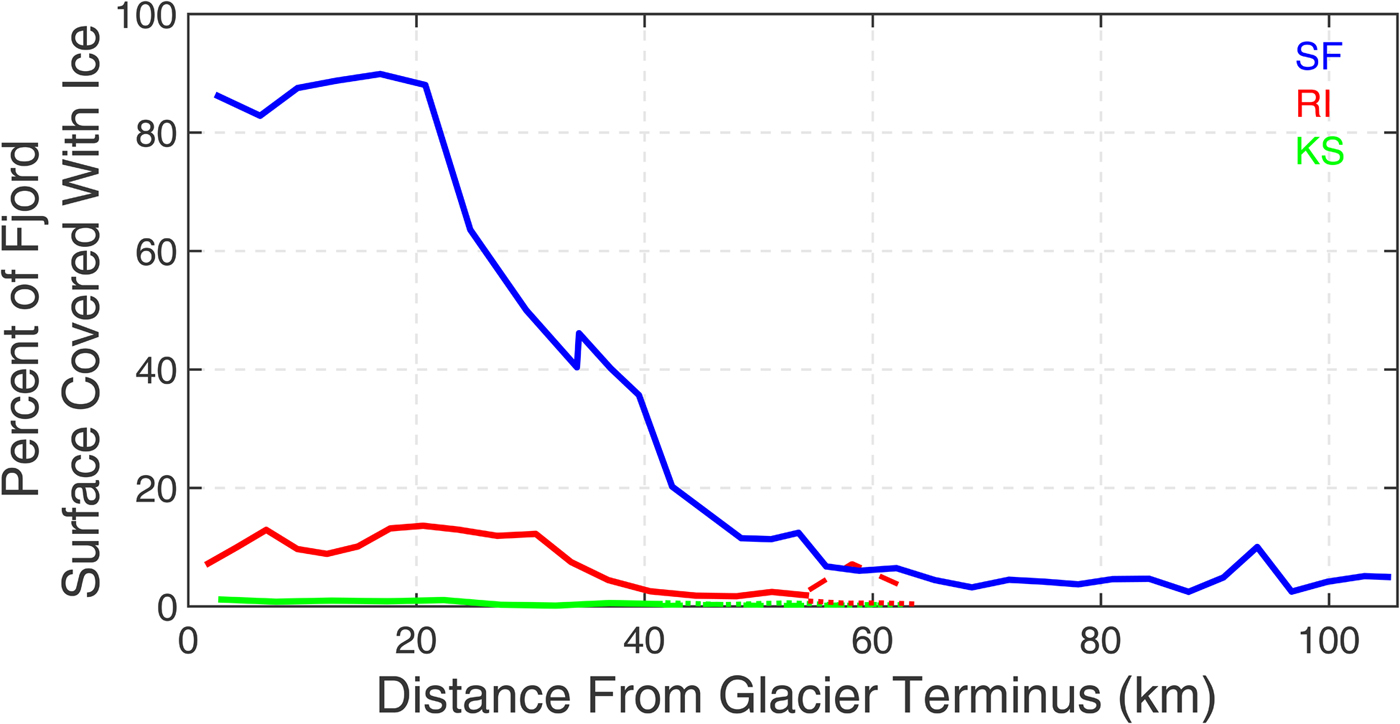
Fig. 4. Average percentage of fjord surface covered in ice for all images analyzed. In RI and KS, dashed lines represent the northern arms of the fjords, while dotted lines represent the southern arms. For temporal variability in percent ice cover from all images analyzed, see Figure S3.
In the Uummannaq region, RI total ice coverage ranged from 1.11 to 23.12% of the fjord surface. Two regions had ice concentrations higher than in the remainder of the fjord: near the glacier terminus and in the north arm of the split (Fig. 4, Figs S1, S3). Ice concentrations in RI were notably higher to the north than the south, suggesting that the majority of ice flows outward through the northern half of the fjord and/or that ice becomes grounded on the shallower sill there and thus spends more time in that region. KS had <2% of its surface covered with ice in all images (Table 1). Ice coverage was highest near the glacier terminus and coverage was slightly higher in the south arm of the fjord than the north (Fig. 4, Fig. S1).
The total iceberg portion that we classified ranged from 16 to99% of the total area of ice coverage (Table 1). Ice that was not classified was either ice in ice mélange that did not have boundaries that were detected by our method, single pixels that were above the brightness threshold for ice but were not adjacent to any other ice pixels, or classified icebergs that were subsequently removed to account for sea ice that was incorrectly categorized by our thresholding method.
Total volumes of classified icebergs were 2.4–7.5 km3 in SF, 1.0–2.0 km3 in RI and 0.04–0.30 km3 in KS (Table 1). In all three fjords, we calculated greater total volumes of ice in images from earlier in the summer (Fig. 5). We fit linear regressions to data of ice volumes versus date, and found the total volume of ice decreases at rates of 0.57 m3 km−2 month−1 in SF between July and late September, and at rates of 0.72 m3 km−2 month−1 in RI and 0.29 m3 km−2 month−1 in KS from mid-July to mid-September. F-tests show that the trend was significantly different from zero in KS (p < 0.001) but not in RI (p = 0.398) or SF (p = 0.400).
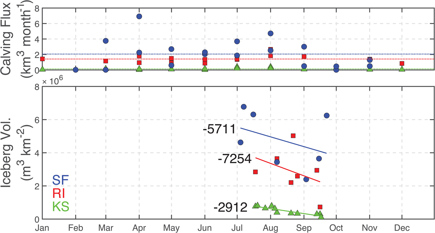
Fig. 5. Monthly calving fluxes (top panel) and total volume of classified icebergs observed in each image where the full fjord was visible (lower panel) throughout the year for SF (blue circles), RI (red squares) and KS (green triangles). Average annual calving fluxes are shown as dotted lines in the upper panel. Linear regression lines of best fit are shown on the lower panel and are annotated with their slopes (m3 km−2 month−1).
Comparisons with manual classification of ice mélange reveal that the SFS method tends to split large icebergs into several smaller icebergs (Table S2). Thus, we used a combination of the automatic SFS method combined with manual delineation for the larger icebergs. We were unable to use the manual delineation method to define a general correction factor for the automatic SFS method, as the resolution of L8 images is too low to accurately delineate all icebergs, and especially small icebergs, present in the ice mélange. Iceberg volumes reported for areas of ice mélange are therefore lower bounds on the total ice present as the sum of the volumes of several small icebergs is less than the volume of a single large iceberg covering the same area.
Iceberg characteristics
SF had the widest range of iceberg properties seen in the three fjords, with lengths of individual icebergs in the range 30–2550 m, yet also had the lowest average iceberg length at 67 m. KS had the smallest range of iceberg lengths (30–780 m) and the smallest maximum iceberg size, yet the highest average iceberg length at 84 m. RI had relatively large iceberg lengths (30–1940 m), with an average length equal to 74 m. Individual iceberg areas ranged to 5.6 × 10⁵ m2 in SF, to 9.5 × 10⁵ m2 in RI and to 1.9 × 10⁵ m2 in KS. The average area of icebergs in SF, RI and KS was 2360, 3670 and 4510 m2, respectively (Table 2).
Table 2. Iceberg size and depth ranges for all images analyzed of SF, RI and KS

Iceberg keel depth estimates were found to be in the range 28–260 m, 28–300 m and 28–190 m in SF, RI and KS, respectively, for block type icebergs (Table 2). For inverted cones, maximum depth estimates were truncated at glacial terminus depths (600 m in SF, 840 m in RI and 250 m in KS) for 0.037, 0.009 and 8.6% of icebergs in SF, RI and KS, respectively. All three fjords had substantial proportions (1–27% in SF, 2–28% in RI and 5–37% in KS) of icebergs reaching depths >100 m, below which fjord waters begin to warm (Fig. 6).
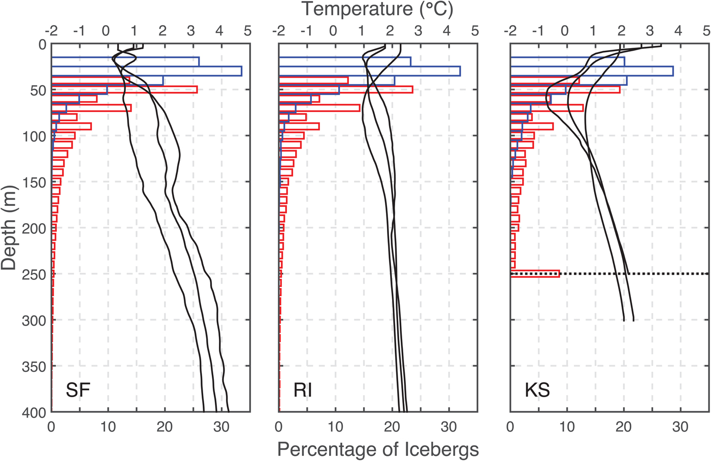
Fig. 6. Percentage of icebergs reaching various depths (bars) and average temperature at depth during three separate summer seasons (black lines) for SF (left), RI (center) and KS (right) fjords. Blue bars represent minimum depths (block shape icebergs) and red bars are maximum depths (cone shaped icebergs). The depth of the grounding line at KS is shown as a dotted line in the right panel.
Iceberg size distributions
By number, small icebergs dominated in all three fjord, but larger icebergs accounted for more of the total volume (Fig. 7). The smallest icebergs (<105 m3, ~65 m long) typically made up more than two thirds of the total number of icebergs in all three fjords, but accounted for <10% of the total ice volume. By contrast, icebergs larger than 107 m3 (~400 m long) accounted for just 0.28%, 1.4% and 0.49% of the number of icebergs but 29%, 58% and 14% of the total volume in SF, RI and KS, respectively (Fig. 7).
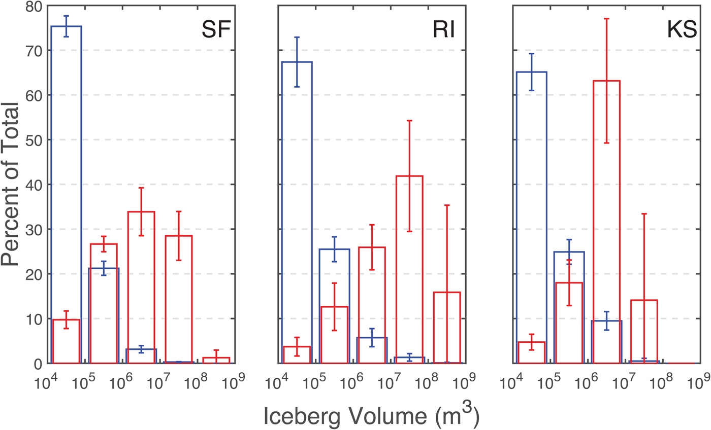
Fig. 7. Average (bars)±one standard deviation (error bars) of the total count (blue) and total volume (red) of classified icebergs across all images of SF (left), RI (center) and KS (Right).
Iceberg area distributions followed power laws with slopes of −2.00 ± 0.06 for SF icebergs delineated via the thresholding method, −1.90 ± 0.06 for SF icebergs delineated using the SFS method (icebergs in mélange), −1.87 ± 0.05 for RI icebergs delineated via thresholding, and −1.62 ± 0.04 for KS icebergs delineated using thresholding (Fig. 8). Power laws were calculated with only a subset of each region's total iceberg area range to achieve a fit to observed distributions with 95% confidence (ranges given are confidence limits for 95% significance). The specific iceberg areas used were 2–113 × 103 m2 for threshold delineated icebergs and areas of 1–88 × 103 m2 for SFS delineated icebergs in SF, 2–51 × 103 km2 in RI and 1–25 × 103 m2 in KS (Fig. 8).
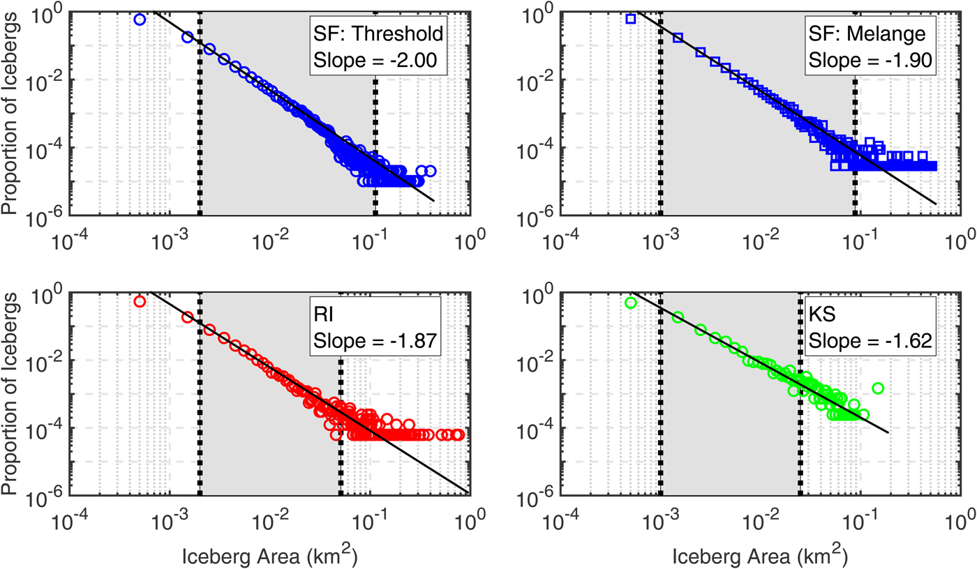
Fig. 8. Observed iceberg distributions (open symbols) and power law predictions (black lines) of the proportion of icebergs of different size classes. Confidence intervals for power law fits are given in the main text. Shaded areas represent the interval over which data match power law distributions with 95% confidence.
We tested the ability of lognormal, Generalized Pareto and Weibull distributions to describe observed distributions of icebergs. Kolmogorov–Smirnov tests revealed that these alternative distributions did not significantly match our observations, even over the more limited ranges than where power laws were statistically significant.
Ice calving flux
Ice calving flux was highest from Helheim Glacier into SF (24 km3 a−1), relatively high into RI (17 km3 a−1) and low into KS (1.6 km3 a−1) (Fig. 5). In all three fjords, a seasonal signal was apparent with low fluxes throughout the winter, and higher than average calving fluxes occurring in the summer months, most notably in August. In the spring of both years in SF we observed 1 month with a high calving flux during the transition between lower winter calving rates and higher summer rates (45 km3 a−1 in March 2013 and 83 km3 a−1 in April 2014) (Fig. 5).
Iceberg trackers
Of all 25 trackers placed in SF, 13 transmitted positions throughout the fjord and eventually exited (Fig. S2). All 13 icebergs tracked that exited the fjord did so in under a year from the date they were tagged. For those 13 icebergs the average residence over the entire fjord was 132 days. Average residence time in the proglacial mélange for the 12 icebergs that we tracked there was 70 days, though note that we did not track these icebergs starting at Helheim Glacier, but rather 3–15 km down-fjord from the calving face. For the 13 icebergs that traversed the entire north-south portion of the fjord (20 km from Helheim Glacier) the average residence time was 62 days.
In RI, two of the trackers that were placed on icebergs traversed the entire fjord and exited via the northern arm, while the third was lost after just two days. Residence times of the two tracked icebergs were 24 and 103 days. Both icebergs recirculated in the region between the glacier terminus and 16 km down-fjord of the terminus, spending 13 and 8 days there. One of the icebergs subsequently exited 11 days after leaving that area. The other recirculated for 44 days in the broad region between 35 and 64 km down-fjord before spending 51 days in the north arm of the fjord where it was likely grounded on the shallow (~240 m) sill and eventually exiting (Fig. S2).
In KS, two icebergs that were tracked in 2013 traversed through the entire fjord and exited the north arm after 11 and 21 days. In 2014 four trackers were deployed, one of which only transmitted data for 2 days so its data are excluded. The remaining three icebergs recirculated within 20 km of the glacier, spending 17, 64 and >35 days there (the tracker that was in the zone for 35 days stopped transmitting before leaving the area). Two of the icebergs then traveled down-fjord and one entered the southern arm of the fjord after 5 days, then stopped transmitting, while the other recirculated in the region between 20 and 30 km down-fjord for 20 days before entering the south arm and stopping transmissions 8 days later (Fig. S2).
DISCUSSION
Fjord ice volumes
To calculate iceberg volume from our observations of iceberg area, we used an area to volume conversion. To compare results with other studies, however, we also fit an empirical relationship between iceberg length (L) in meters and mass (M) in tonnes for 712 icebergs using the power law:
 $$M = aL^b $$
In our relationship, a = 2.35, b = 2.55 and the correlation coefficient R 2 = 0.93. These results are similar to those of Hotzel and Miller, (Reference Hotzel and Miller1983) (a = 2.009, b = 2.68, R 2 = 0.90) who used 168 icebergs observed off Labrador and Barker and others (Reference Barker, Sayed and Carrieres2004) (a = 0.43, b = 2.9, R 2 = 0.92) who used 14 measurements of nine icebergs observed in waters around Labrador by Smith and Donaldson, (Reference Smith and Donaldson1987). These similarities suggest a robust relationship that can be applied to icebergs produced by calving glaciers in other Arctic regions. Whether or not the trend of a lower value of the exponent b inside the glacial fjords compared with offshore Labrador is physically meaningful will have to be tested by a future study. This could imply that icebergs become more cube-like as they age and transit the North Atlantic.
The amount of ice per surface area of fjord water decreased in all three fjords between spring and late summer (Fig. 5). Decreases in ice coverage could be the result of decreased input from calving glaciers, increases in ice export out of fjords, and/or increased melt of icebergs and sea ice within fjords. We rule out decreased calving fluxes as we observed calving to be steady or increase over the same time period in each fjord (Fig. 5). Reductions in sea ice are also unable to account for the observed decrease in ice volume. Analysis of Worldview images show that the contribution of sea ice to total ice amount decreased by 1.4% between July and late August in SF, and 1.9% per month between mid-July and mid-August in RI. Total ice volumes calculated from L8 images decreased by 10–20% over the same timeframe.
Increases in export and melting likely both contribute to decreased total iceberg volume. In the winter, sea ice forms in RI and KS as well as outside of all three fjords (reaching a maximum in the early spring), effectively blocking export of icebergs from the fjords and leading to a buildup of icebergs. Break-up of sea ice in the late spring and summer allows the buildup of ice to be cleared resulting in a decrease in total ice volume. Additionally, freshwater runoff from the GrIS increases in summer causing stronger net down-fjord flow (Bamber and others, Reference Bamber, Van Den Broeke, Ettema, Lenaerts and Rignot2012; Box and Colgan, Reference Box and Colgan2013; Bartholomaus and others, Reference Bartholomaus2016; Jackson and Straneo, Reference Jackson and Straneo2016). Increased runoff may also cause higher rates of iceberg melt, as runoff can take the form of subsurface plumes with positive temperature anomalies that flow down-fjord at depths containing iceberg keels (Carroll and others, Reference Carroll2015; Cowton and others, Reference Cowton, Slater, Sole, Goldberg and Niewnow2015).
Using standard residence time calculations, we obtained first order approximations of ice fluxes using our measurements of total ice volume and tracked iceberg residence times. Using the equation
 $${\rm Ice}\,{\rm Flux =} \displaystyle{{{\rm Total}\,{\rm Ice}\,{\rm Volume}} \over {{\rm Ice}\,{\rm Residence}\,{\rm Time}}}$$
and average total ice volumes and residence times for each fjord we estimate ice fluxes of 18, 9.6 and 2.5 km3 a−1 for SF, RI and KS, respectively. These estimates are generally consistent with ice fluxes measured from glacier speed and terminus change data of 24, 17 and 1.6 km3 a−1, and demonstrate that we can obtain reasonable estimates of either ice flux, volume, or residence time if data for the other two properties are available.
Iceberg classification
While our method is able to quantify many of the icebergs seen in L8 images, we cannot classify all ice for two primary reasons: the difficulty of finding and connecting discrete edges of icebergs within ice mélange, and to a lesser extent the exclusion of very small bits of ice that occupy a single pixel or less of the images.
Ice mélange was most prevalent in SF: a persistent proglacial mélange existed in all available images, typically occupying the majority of the first 20 km of the fjord. In the images used in this study, we classified 4.7–39% of the total ice area in the mélange as icebergs. Despite the fact that our method splits up some large icebergs, we observe a larger average area of icebergs in the ice mélange (3.6 × 10² m2) compared with those in the remainder of the fjord (2.2 × 10² m2). Icebergs deteriorate through mechanical breakup and melt within fjords, so the largest icebergs will typically be found near parent glaciers (Kubat and others, Reference Kubat, Sayed, Savage, Carrieres and Crocker2007; Enderlin and Hamilton, Reference Enderlin and Hamilton2014; Wagner and others, Reference Wagner2014). Additionally, ice mélange has been shown to exert a back-stress sufficient to prevent calving from glacier termini (Amundson and others, Reference Amundson2010). Similar processes may prevent the breakup of large icebergs in mélange.
The volume of icebergs delineated in ice mélange by our automated classification process was on average 76% of the volume delineated manually (Fig. 2). To estimate the volume of ice unaccounted for by the misclassification of large icebergs as smaller icebergs, we assumed that the calculated volume of classified icebergs is 76% of the actual volume of those icebergs. In the DEMs used for area/volume relationships, ice in mélange that was not part of large icebergs generally had a freeboard height of <1 m. We therefore used an upper bound of 10 m for thickness of unclassified ice in mélange and calculate a volume of unclassified ice based on that thickness. Under these assumptions, we estimate that we were able to classify an average of 48% of the total ice mélange volume as icebergs (Table 3). This is likely an underestimate, as much of the ice in ice mélange is thin bergy bits and brash ice that has a thickness of <10 m.
Table 3. Estimated volumes of ice mélange that was not classified as icebergs in SF
Growlers, bergy bits and brash ice, collectively defined as pieces of ice smaller than 15 m in length (Canadian Ice Service, Reference Fequet2005), account for a portion of total ice area found using the threshold method that we did not include in our iceberg analyses. The area of this small ice that was removed ranged from 0.3 to 1.5%, 0.3–5.6% and 0.8–3.8% of the total ice area in images from SF, RI and KS respectively (Table 1). Even assuming a generous average depth of 10 m for these small bits of ice, the volume of this removed ice is below 1% of the calculated volume of classified icebergs in all images.
Iceberg distributions
The exponents of power laws that describe iceberg size distributions relate to the relative abundance of icebergs within different size classes. Exponents that are more negative suggest a higher relative abundance of small sized icebergs (Fig. 9). We interpret the differences in exponents to arise from differences in glacier calving style and total ice flux in each fjord.
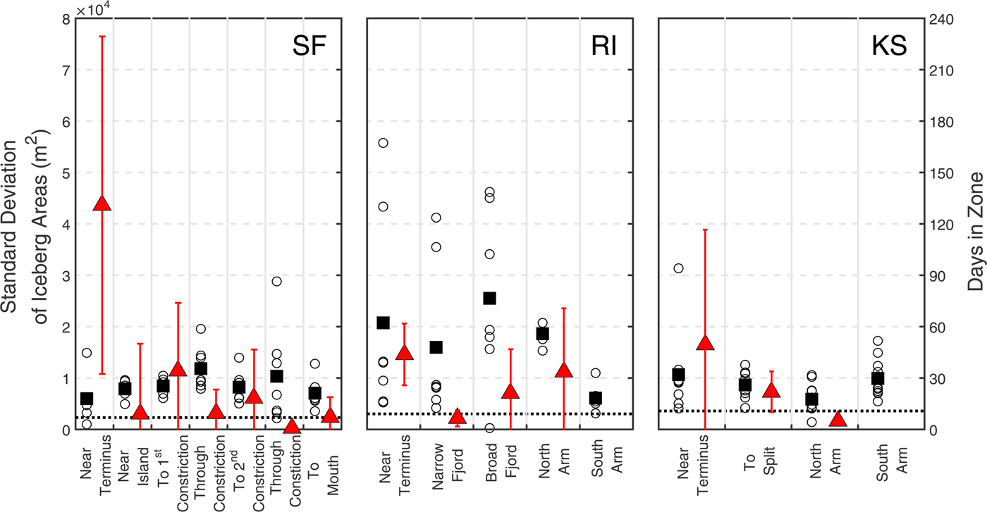
Fig. 9. Iceberg size variability and down-fjord speed in geographic zones in SF (left), RI (center) and KS (right). Zones are indicated in Figure S2. Standard deviation of iceberg areas is displayed for each image (black circles), and the average standard deviation is shown (black squares). Average iceberg area is shown (black dotted line) for reference. Red triangles represent average down-fjord speed of tracked icebergs in each zone. Red error bars are ±1 standard deviation in SF and KS and represent the range of values in RI where data consists of two icebergs only. No tracked icebergs traversed the southern arms of RI or KS, hence no data are presented for iceberg speeds in those zones.
The smallest average iceberg size and the most negative power law exponents, were observed in SF (Fig. 8). Calving from Helheim Glacier is dominated by large-scale calving events over its entire depth (~600 m) as buoyant forces lift the terminus, which may be held below flotation by its attachment to the rest of the glacier, and cause icebergs to calve with a bottom-out rotation (James and others, Reference James, Murray, Selmes, Scharrer and Leary2014; Murray and others, Reference Murray2015). This calving style results in ice rising quickly from depth, and in SF this ice rises into a tightly packed mélange where collision with other ice is likely. Several mechanisms may act to cause this small average iceberg size in Sermilik Fjord. First, continued collisions and friction between icebergs transiting the mélange may be responsible for additional breakdown of large icebergs into smaller pieces. Second, icebergs also move slowly through the mélange, spending more than 70 days there on average, allowing time for melting. SF has the highest water temperatures of the three fjords (near 0°C at the surface to 4.5°C at >400 m depth (Fig. 6)), and continued melting of transiting and circulating icebergs may also contribute to the lower average size of icebergs in the fjord (Straneo and others, Reference Straneo2010; Sutherland and others, Reference Sutherland, Straneo and Pickart2014b). Finally, since Helheim is largely grounded, it may be a prolific producer of numerous smaller-sized icebergs.
Power law exponents from RI suggest that icebergs breakdown following similar processes as in SF, rather than KS (Fig. 8), though iceberg sizes vary to a greater degree in RI than either of the other fjords (Fig. 9). The wider range of overall sizes may be a consequence of two separate calving processes: small-scale events that occur with high frequency and lead to detachment of non-tabular icebergs, most frequently from crevassed areas of the glacier; and large-scale events in which large tabular icebergs calve from the least crevassed portion of the glacier as buoyant forces act on portions of the glacier that are held below flotation and cause fracturing (Medrzycka and others, Reference Medrzycka2016). While the second mechanism is similar to the dominant style of calving in SF, icebergs calved in this manner in RI do not regularly roll as they calve, and generally do not calve into a compact ice mélange in summer. Icebergs in RI may therefore be subject to less fragmentation via collisions and grinding against other icebergs. We do observe an ephemeral ice mélange in RI when, after a large calving event, a temporary mélange made up of icebergs, bergy bits and sea ice, travels down-fjord staying in close proximity, potentially enhancing breakdown via collision (e.g., Fig. 1a).
In RI, high concentrations of ice occurred near the head of the fjord, throughout the north of the narrow section of the fjord and behind the sill north of the island (Fig. S1). High concentrations to the north may indicate the influence of rotation on surface and subsurface waters flowing down-fjord, which is also suggested by the trajectories of tracked icebergs (Fig. S2). High ice concentrations to the north of the island are likely the result of larger icebergs reaching depths exceeding the depth of the sill and becoming grounded, as did one of the tracked icebergs. Notably, we observed that the variability in iceberg areas decreased with increasing distance from the glacier terminus (Fig. 9). We attribute this decrease in variability to the fracture of the largest icebergs as they traverse the fjord, which results in more uniform pieces of ice with distance from the glacier terminus.
Total ice coverage in KS was too low to reveal any strong spatial or temporal patterns, but comparisons with RI and SF do reveal interesting contrasts. In KS, variability in iceberg areas, which we approximate using the standard deviation of iceberg areas, is the lowest of the three fjords and most consistent throughout the fjord (Fig. 9). The average iceberg area was largest in KS despite the glacier having the shallowest grounding line of the three. We attribute the consistency and larger size to a less dynamic style of calving where ice is not rolling and rising from great depths and therefore remains more intact. The low concentrations of ice also allow less chance of icebergs grinding or knocking together and subsequently breaking into smaller pieces. Water in KS is also colder at equivalent depths than in SF or RI leading to less melting (Fig. 7). Finally, though our data are limited, observed residence times of icebergs were lower in KS than the other two fjords, allowing less time for iceberg deterioration during transit through the fjord.
While the general shape of iceberg distributions in the three fjords was accurately described by power laws, these distributions fail to predict the very large icebergs, which can represent a significant proportion of total iceberg volume. Maximum observed individual iceberg volumes averaged 1.6 × 10⁸, 2.4 × 10⁸ and 1.6 × 10⁸ m3 in SF, RI and KS, respectively. Each of these maximum size icebergs falls outside the statistically significant power law fit found here, implying the need to carefully consider the addition of icebergs outside the range of the statistically significant distributions for use in models that include icebergs. Despite being rare in number, these largest icebergs that represent a significant portion of total iceberg volume, have the largest amounts of ice reaching to depths that contain warmer waters (Fig. 7) and the highest potential to exit the fjord. Since models (e.g., Stern and others, Reference Stern, Adcroft and Sergienko2016) are beginning to resolve these largest icebergs, care should be taken when parameterizing iceberg size distributions in models to account for the largest size classes.
Across the three fjords we observed power law exponents that are similar to the −2.0 reported for icebergs in the mélange of SF (Enderlin and others, Reference Enderlin, Hamilton, Straneo and Sutherland2016) and more negative than the −3/2 reported for Antarctic icebergs (Tournadre and others, Reference Tournadre, Bouhier, Girard-Ardhuin and Rémy2016). The difference between the distributions of Greenlandic and Antarctic icebergs highlights the importance of different breakdown mechanisms. In fjords with more productive glaciers (SF and RI) a greater proportion of small icebergs may be produced during calving, and/or high iceberg concentrations may cause greater fracture and breakdown as discussed above. In KS where iceberg concentrations are low breakdown processes will be more similar to those controlling the distributions of icebergs in open ocean, as exemplified by a more similar exponent to Antarctic distributions in KS (−1.62).
These results demonstrate the potential of observed iceberg distributions to act as a fingerprint of glacier productivity and calving style in fjords. More productive glaciers with deeper grounding lines tend to have more negative power law exponents than smaller less productive glaciers. While power laws under-predict the largest iceberg sizes in fjords, combined iceberg volume may be over-predicted outside of mélange regions in fjords with substantial ice mélange. Power laws more sufficiently cover the range of observed icebergs in fjords with smaller glaciers (Fig. 8). Future work could include examining a system before and after a significant retreat that resulted in a change in grounding line depth and/or adding to the number of systems examined here to test if these relationships hold.
Keel depths and melt
Icebergs reaching deeper, warmer fjord waters have the potential to affect subsurface water properties because of their direct freshwater contribution and their ability to entrain ambient water as the buoyant melt rises upwards. The melting of icebergs is analogous to the subaqueous melting of glacial termini, which has been investigated using observations, numerical modeling and laboratory experiments (e.g., Eijpen and others, Reference Eijpen, Warren and Benn2003; Jenkins, Reference Jenkins2011; Xu and others, Reference Xu, Rignot, Menemenlis and Koppes2012). We expect submarine melting of icebergs to be akin to the ambient melting of glacier termini, which create melt rates that are lower than the enhanced melting that occurs in the presence of subglacial discharge plumes (e.g., Motyka and others, Reference Motyka, Hunter, Echelmeyer and Connor2003; Jenkins, Reference Jenkins2011; Cowton and others, Reference Cowton, Slater, Sole, Goldberg and Niewnow2015; Carroll and others, Reference Carroll2016).
We calculated the total submerged surface area of icebergs at different depths based on block shaped icebergs. Our estimates of submerged surface area of icebergs exceed that of the glacier faces (grounding line depth multiplied by glacier width) by at least one order of magnitude throughout all three fjords (Table 4).
Table 4. Water temperature and average surface area (km2) of ice at depth. Temperatures are averages of measurements taken throughout each fjord over three summers. Iceberg areas assume that icebergs maintain their cross-sectional area at the water line throughout their depths
Icebergs have the greatest potential to modify subsurface water properties in SF because of the high concentration of icebergs and relatively high water temperatures. Water temperature in SF increases below the surface layer, reaching temperatures of 2°C at 200 m and rising to 3.5°C at 400 m in summers (Fig. 6) (Sutherland and others, Reference Sutherland, Straneo and Pickart2014b). Enderlin and others (Reference Enderlin, Hamilton, Straneo and Sutherland2016) calculated average summertime melt rates in the ice mélange in SF of 0.12 m d−1 (range 0.05–0.23 m d−1) for shallow-keeled icebergs and 0.40 m d−1 (range 0.31–0.67 m d−1) for deep-keeled icebergs. Applying those rates to submerged iceberg surface areas in SF, using a cutoff depth of 118 m for shallow vs deep keels (Enderlin and others, Reference Enderlin, Hamilton, Straneo and Sutherland2016), yields a freshwater contribution from iceberg melt of 620 ± 140 m3 s−1 to the fjord, with 240 ± 90 m3 s−1 inside the mélange and 380 ± 120 m3 s−1 outside the mélange region. These calculations are similar to other estimates of mélange melt of 214–823 m3 s−1 (Enderlin and others, Reference Enderlin, Hamilton, Straneo and Sutherland2016) and combined iceberg and glacier face melt of 1000–2000 m3 s−1 (Jackson and Straneo, Reference Jackson and Straneo2016), though our estimates are likely to underestimate the total freshwater flux because we exclude icebergs with lengths <30 m.
CONCLUSIONS
Icebergs are a significant component of total freshwater discharge from Greenland. This work represents the first attempts to describe iceberg characteristics and examine how they vary in Greenland. We used satellite data to quantify the first fjord-wide distributions of iceberg sizes and total ice coverage in three fjords. We constructed DEMs using high resolution satellite imagery and described a relationship between iceberg areas and volumes (V = 5.96A 1.30). We used that area to volume relationship to quantify the total volume of ice present in fjords, accounting for sea-ice contamination, and to estimate iceberg keel depths and subsurface iceberg surface area.
We found substantial differences in iceberg characteristics between the three fjords that we investigated. Variability is tied to differences in glacier grounding line depths, calving styles and fjord water properties and circulation. These differences are captured by exponents of power laws fit to observed iceberg size distributions, with exponents equal to −1.95 ± 0.06, −1.87 ± 0.05 and −1.62 ± 0.04 in Sermilik Fjord, Rink Isbræ and Kangerlussuup Sermia fjords, respectively. Additionally, these distributions suggest fundamental differences between processes controlling the breakdown of Greenlandic and Antarctic icebergs.
The new method developed here represents a significant first step towards quantifying iceberg properties on large scales and quantifying freshwater input from iceberg melt throughout Greenland. Future study includes applying these methods to other fjords, exploring the use of radar rather than optical satellite observations to obtain year-round coverage, using these distributions to seed icebergs in numerical ocean models, and refining estimates of iceberg keel depths, subaqueous surface areas and freshwater input from iceberg melt. This work highlights the need for more observations of iceberg keel shapes and depths. Expanding records of surface currents through continued use of icebergs as drifters or other means, as well as obtaining measurements of water properties and circulation within other fjords is also necessary to continue and expand this work.
SUPPLEMENTARY MATERIAL
The supplementary material for this article can be found at https://doi.org/10.1017/aog.2017.5.
ACKNOWLEDGEMENTS
We dedicate this paper to Gordon Hamilton. Funding was provided by NASA grant NNX12AP50G and National Science Foundation grant 1552232, with partial support from the University of Oregon. WorldView images were distributed by the Polar Geospatial Center at the University of Minnesota (http://www.pgc.umn.edu/imagery/) as part of an agreement between the US National Science Foundation and the US National Geospatial Intelligence Agency Commercial Imagery Program. We thank Laurie Padman and two anonymous reviewers for constructive comments and suggestions. Code for generating the iceberg distributions and analysis presented here is available by contacting the authors.


 Open access