


1. INTRODUCTION
The grounding zone, where ice transitions from grounded to freely floating, is a narrow but crucial portion of marine ice sheets. Ocean tides beneath the ice shelf lead to ice flow modulation far upstream of the grounding line (Anandakrishnan and others, Reference Anandakrishnan, Voigt and Alley2003; Bindschadler and others, Reference Bindschadler, King, Alley, Anandakrishnan and Padman2003; Gudmundsson, Reference Gudmundsson2006) and the flexure of ice in this region can be used as an indicator of grounding line (GL) position (Goldstein and others, Reference Goldstein, Engelhardt, Kamb and Frolich1993; Rignot, Reference Rignot1998a, Reference Rignotb; Sykes and others, Reference Sykes, Murray and Luckman2009; Rignot and others, Reference Rignot, Mouginot and Scheuchl2011) and migration (Brunt and others, Reference Brunt, Fricker and Padman2011). Ice-sheet mass balance is often estimated as the difference between net accumulation upstream of the GL and mass flux across it but this calculation is sensitive to uncertainty in the GL position and ice thickness at the GL (Shepherd and others, Reference Shepherd2012).
Studies of ice-shelf tidal flexure have been used frequently to seek insights into ice rheology and determine GL position based on a given flexure profile. Ice in the grounding zone bends to accommodate the vertical motion of the adjoining ice shelf resulting from ocean tides. In the past this has typically been modelled as some form of elastic beam/plate equation (Holdsworth, Reference Holdsworth1969, Reference Holdsworth1977; Lingle and others, Reference Lingle, Hughes and Kollmeyer1981; Smith, Reference Smith1991; Vaughan, Reference Vaughan1995; Schmeltz and others, Reference Schmeltz, Rignot and MacAyeal2002; Sykes and others, Reference Sykes, Murray and Luckman2009; Sayag and Worster, Reference Sayag and Worster2011, Reference Sayag and Worster2013; Walker and others, Reference Walker2013; Marsh and others, Reference Marsh, Rack, Golledge, Lawson and Floricioiu2014; Hulbe and others, Reference Hulbe2016). Some of these studies seek to determine the elastic (Young's) modulus of glacial ice in situ by matching beam theory to observed flexure profiles (e.g. Lingle and others, Reference Lingle, Hughes and Kollmeyer1981; Stephenson, Reference Stephenson1984; Kobarg, Reference Kobarg1988; Smith, Reference Smith1991; Vaughan, Reference Vaughan1995; Schmeltz and others, Reference Schmeltz, Rignot and MacAyeal2002; Sykes and others, Reference Sykes, Murray and Luckman2009; Hulbe and others, Reference Hulbe2016) as an alternative to seismic or mechanical laboratory experiments (e.g. Jellinek and Brill, Reference Jellinek and Brill1956; Dantl, Reference Dantl1968; Roethlisberger, Reference Roethlisberger1972; Hutter, Reference Hutter1983; Rist and others, Reference Rist1996; Petrenko and Whitworth, Reference Petrenko and Whitworth2002). Alternatively, assumptions about ice rheology have been made in order to invert tidal flexure curves for ice thickness in the grounding zone (Marsh and others, Reference Marsh, Rack, Golledge, Lawson and Floricioiu2014). Finally, (D)InSAR (Differential Interferometric Synthetic Aperture Radar) has become a common tool to determine GL position, either through fitting an elastic beam model to tidal fringes (Rignot, Reference Rignot1998a, Reference Rignotb; Sykes and others, Reference Sykes, Murray and Luckman2009) or by positioning it at the location in a differential interferogram where vertical motion is detected above noise for the first time (Rignot and others, Reference Rignot, Mouginot and Scheuchl2011). Here, we question the validity of some of the approaches listed above.
Ice stiffness, typically described by the Young's modulus (E), is important for the transmission of elastic stresses through ice and is a crucial parameter when considering its fracture or damage. Elastic stresses play a key role in the propagation of (relatively) high frequency tidal motion through ice (Gudmundsson, Reference Gudmundsson2007, Reference Gudmundsson2011; Walker and others, Reference Walker, Christianson, Parizek, Anandakrishnan and Alley2012; Thompson and others, Reference Thompson, Simons and Tsai2014; Rosier and others, Reference Rosier, Gudmundsson and Green2015; Rosier and Gudmundsson, Reference Rosier and Gudmundsson2016) and any weakening in shear margins due to crevasses could partly explain the large distances upstream that these signals are observed (Thompson and others, Reference Thompson, Simons and Tsai2014). Ice stiffness is also an important parameter for the fracture toughness of ice. Estimates of this parameter obtained by fitting a beam model to flexure profiles have recently been used to model strand crack formation in the grounding zone (Hulbe and others, Reference Hulbe2016).
Direct comparisons cannot be made between laboratory measurements of ice elasticity and those obtained from fitting models to ice-shelf flexure profiles, as ice is not purely elastic over tidal timescales (Schmeltz and others, Reference Schmeltz, Rignot and MacAyeal2002; Reeh and others, Reference Reeh, Christensen, Mayer and Olesen2003; Wild and others, Reference Wild, Marsh and Rack2017). The true elastic modulus and the ‘effective’ modulus observed in the field are material properties of two separate rheological models. In reality, deformation of ice crystal fabric and change in bulk structure due to accumulated strain leads to a nonlinear variation in strain rate and an overall softening of the ice over time. This cannot be observed in the instantaneous elastic response. As well as providing a misleading Young's modulus, a purely elastic model of ice at tidal timescales can only transmit stresses instantaneously with no phase lag. In contrast, while still not matching all time-dependent changes in ice fabric, a realistic viscoelastic rheology incorporates the delayed viscous signal, which changes ice stream response to tidal forcing and leads to long-period modulation in velocity (Rosier and Gudmundsson, Reference Rosier and Gudmundsson2016).
In the discussion that follows we will use the term ‘effective’ ice stiffness to denote the apparent ice stiffness that would be inferred from a simple interpretation of flexural profiles, as has been done frequently in the past. In reality, the Young's modulus is a material parameter that should not change as a result of crevassing (but could be altered by changes in ice temperature or fabric). It is well established that ice damage can cause a change in the ‘effective’ ice rheology. This is often accounted for using a continuum damage mechanics approach, which introduces a damage parameter into the rheological equation for ice (Pralong and others, Reference Pralong, Funk and Lüthi2003; Pralong and Funk, Reference Pralong and Funk2005; Tsai and others, Reference Tsai, Rice and Fahnestock2008; Borstad and others, Reference Borstad2012; Thompson and others, Reference Thompson, Simons and Tsai2014). Here, we adopt the alternative approach of directly including the crevasses in our model geometry, as has been done by Freed-Brown and others (Reference Freed-Brown, Amundson, MacAyeal and Zhang2012).
In this study we explore factors that influence flexure that have been previously ignored and how these factors could change the interpretation of ice rheology. A quantitive analysis of the effects of crevassing and vertical density variation on the tidal flexure of ice in the grounding zone are investigated for the first time. We compare results between a linear elastic beam model and a 2-D full-Stokes viscoelastic finite element model that has been used in the past to explore ice/tide processes (Gudmundsson, Reference Gudmundsson2011; Rosier and others, Reference Rosier, Gudmundsson and Green2014, Reference Rosier, Gudmundsson and Green2015; Rosier and Gudmundsson, Reference Rosier and Gudmundsson2016). The model domain is based on a comprehensive recent survey of the grounding zone of White Island on the Southern McMurdo Ice Shelf, including ice thickness measurements and locations of probable basal crevasses obtained by radar (Fig. 1). This extensive dataset provides a unique opportunity to investigate flexural processes in far more detail than has previously been possible. We show that using a linear elastic beam model to study a nonlinear viscoelastic process can provide an excellent fit to flexure profiles, provided any phase information is ignored. This flexibility of the elastic beam theory to successfully replicate observations should however not been taken as indication of the correctness of the rheological model on which the linear elastic beam theory is based. We show that even if ice thickness is known, the presence of basal crevasses can greatly alter the flexure profile, which would be misinterpreted as a change in Young's modulus. Considerable care should be taken when interpreting ice-shelf flexure profiles to determine ice rheology or thickness. In contrast, using flexure profiles to determine GL position is reasonably robust depending on the level of accuracy required.

Fig. 1. Differential interferogram from the Southern McMurdo Ice Shelf study site, derived from three TerraSAR-X scenes in 2014, showing the flexure zone as dense band of fringes. Each fringe corresponds to 2.2 cm of vertical displacement. Background image is a Landsat 8 scene from 23 February 2017. Also marked is the grounding line (solid black line), model domain (solid white line), radargram line (dashed black line), 30 m ice speed contours (dashed white line) and the location of the firn core (star). Inset shows the extent of the main figure (red box) in the context of the Ross Ice Shelf. Note the location of the shear margin between the Southern McMurdo and Ross Ice Shelves, shown by tightly packed ice speed contours. Image courtesy DLR.
2. METHODS
The full-Stokes solver MSC.Marc (MSC, 2016) is used to simulate a 20 km flowline (15 km floating, 5 km grounded) of the Southern McMurdo Ice Shelf grounding zone. It uses the finite element method in a Lagrangian frame of reference to solve for conservation of mass, linear momentum and angular momentum:
 $$\displaystyle{{D\rho} \over {Dt}} + \rho v_{i,i} = 0,$$
 $$\sigma _{ij,j} + f_i = 0,$$
 $$\sigma _{ij} - \sigma _{\,ji} = 0,$$
where D/Dt is the material time derivative, ρ is mass density, v i are the components of the velocity vector, σ ij are the components of the Cauchy stress tensor and f i are the components of the gravity force per volume. In this way, unlike most previous studies of tidal flexure, the model does not use any form of thin beam approximation. We use summation convention of dummy indices and the comma to denote partial derivatives, in line with standard Cartesian tensor notation. The model is 2-D plane strain such that all strain components with an across flow (y) term vanish. The deviatoric stress and strain components (τ ij and e ij , respectively) are defined as
 $$e_{ij} = {\epsilon} _{ij} - \displaystyle{1 \over 3}\delta _{ij}{\epsilon} _{\,pp}$$
and
 $$\tau _{ij} = \sigma _{ij} - \displaystyle{1 \over 3}\delta _{ij}\sigma _{\,pp},$$
where ε ij are the components of the strain tensor and δ ij is the Kronecker Delta.
Ice is treated as a Maxwell viscoelastic material. This is a two-element rheological model comprising a viscous damper and an elastic spring connected in series, such that an applied stress yields an instantaneous elastic strain and a time dependent viscous strain. The total deviatoric strain rate $\dot e_{ij}$
is therefore the sum of these two contributions:
$\dot e_{ij}$
is therefore the sum of these two contributions:
 $$\dot e_{ij} = A\tau _{\rm E}^{n - 1} \tau _{ij} + \displaystyle{1 \over {2G}}\mathop {\tau _{ij}} \limits^\nabla,$$
where the dot indicates a time derivative.
The first term on the right-hand side represents the viscous component of deformation where A is the temperature dependent rate factor in Glen's flow law, n is creep exponent (a nonlinear relation with n = 3 is used throughout) and
 $$\tau _{\rm E} = \sqrt {\tau _{ij}\tau _{\,ji}/2} $$
is the effective stress. The second term on the right-hand side of (6) is the elastic component of deformation, where the superscript $\nabla $
denotes the upper-convected time derivative:
$\nabla $
denotes the upper-convected time derivative:
 $$\mathop {\tau_{ij}} \limits^\nabla = \displaystyle{D \over {Dt}}\tau _{ij} - \displaystyle{{\partial v_i} \over {\partial x_k}}\tau _{kj} - \displaystyle{{\partial v_j} \over {\partial x_k}}\tau _{ik},$$
G is the shear modulus:
 $$G = \displaystyle{E \over {2(1 + \nu )}},$$
ν is the Poisson's ratio and E is the Young's modulus (Christensen, Reference Christensen1982). A standard value of 0.3 is used throughout for the Poisson's ratio (Lingle and others, Reference Lingle, Hughes and Kollmeyer1981; Stephenson, Reference Stephenson1984; Kobarg, Reference Kobarg1988; Smith, Reference Smith1991; Vaughan, Reference Vaughan1995; Schmeltz and others, Reference Schmeltz, Rignot and MacAyeal2002; Sykes and others, Reference Sykes, Murray and Luckman2009) and in line with previous studies the effect of changing this is negligible and not discussed further.
We choose to avoid the complication of matching the background flow of the ice stream, largely because the flow in this region is not aligned with the 2-D flexure line that we investigate. Following Thompson and others (Reference Thompson, Simons and Tsai2014) we set the body force f i = 0 in (2). This will only alter the viscous component of our model since the effective viscosity is a function of the effective stress. In this case, since we are only interested in the relative amplitude of the flexure profile and do not investigate its phase, any resulting difference between the two models will be very small. Without the body force there is no need to apply an ocean back pressure at the downstream end of the model, so instead a stress-free condition is applied.
Ice rests on seawater of uniform mass density ρ w = 1030 kg m−3 ,which exerts an ocean pressure normal to the base of the floating ice shelf given by
 $$p_{\rm w} = \rho _{\rm w}gS(t),$$
where g is gravitational acceleration, S(t) is the time varying sea level, consisting of a sine wave of diurnal period with an amplitude equal to the local ocean tide of ~0.3 m. Grounded ice rests on an elastic bed 5 m thick with stiffness k = E t/H t, where E t is the till elasticity and H t is the till thickness. Sayag and Worster (Reference Sayag and Worster2011, Reference Sayag and Worster2013) previously investigated the effects of till stiffness on the flexure profile and we do not expand on this analysis. We briefly show the effect of reducing k in one set of experiments for the sake of comparison, but in general k is fixed to a value of 1 GPa m−1, representing a relatively stiff bed (Sayag and Worster, Reference Sayag and Worster2013) to avoid complicating our results with soft till effects. At the GL ice is pinned to the bed such that the GL cannot migrate, in accordance with DInSAR analysis that shows no GL migration at this site (Wild and others, Reference Wild, Marsh and Rack2017). The GL position used in the model is the GL position as identified in the radargram with the aid of DInSAR interferograms.
It is worth pointing out here that, although the system of equations we solve in our model are very different from the purely elastic beam model, the boundary conditions we employ are almost exactly the same. In his derivation, Holdsworth (Reference Holdsworth1969) assumes that the ice is plane strain, resting on an elastic foundation and clamped vertically at the GL. At the downstream end of the beam the vertical deflection equals vertical tidal motion and its gradients in x are zero. All these conditions are satisfied in our model, provided that the domain is sufficiently long (which we show later in the results).
The model domain consists of an unstructured mesh of ~50,000, 2-D isoparametric triangular elements, refined around the grounding zone leading to a resolution of up to 4 m in this region. Radargrams in this area, obtained during a recent survey, indicate extensive basal crevassing in the grounding zone. In some simulations we manually add cracks into the finite element mesh at locations where we interpret likely basal crevasses based on one of the radargrams across the White Island grounding zone (Fig. 2a). Due to the difficulty in determining crevasse depths from the radargram we adopt the simpler approach of testing two scenarios, with depths chosen to be either 10% or 25% of local ice thickness and crack opening angles (α) of either 1° or 0.001°. An outline of the resulting model geometry, showing crevasse depths of 25% ice thickness and crack opening angles of 1°, is shown in Fig. 2b.
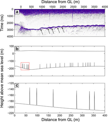
Fig. 2. (a) Radargram across the grounding zone of White Island, Southern McMurdo Ice Shelf, showing extensive basal crevassing (some of the more distinct basal crevasses are indicated by arrows). (b) Outline of the model domain in the grounding zone for a crevassed geometry: a = 0.25 H, α = 1°, where a is the crevasse depth through the ice thickness H and α is the crevasse opening angle. Note that the full model domain extends beyond this region (extent shown in Fig. 1). (c) Close up of the portion of the domain outlined in the red box of panel b, showing details of the crevasse geometry for α = 1°.
A 10 m firn core was taken in the survey area at the same time as radar measurements were made (location shown in Fig. 1). This was divided into 5–10 cm sections, which were weighed and measured to obtain estimates of firn densification (shown in Fig. 3a). These measurements were fitted to an exponential curve assuming glacial ice mass density (ρ ice) of 917 kg m−3 giving the following depth density relation:
 $$\rho _{\rm i}(z) = \rho _{{\rm ice}} - (573\;\exp ( - 0.0529z)).$$
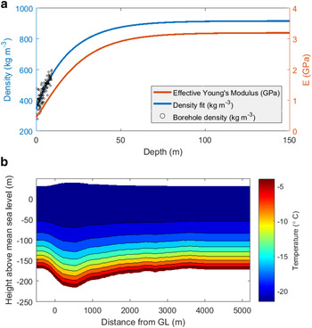
Along with the mass density profile given in (11) we use a simple relation of a form given by Gibson and Ashby (Reference Gibson and Ashby1988) to calculate a depth dependent Young's modulus as
 $$E(z) = \left( {\displaystyle{{\rho _{\rm i}(z)} \over {\rho _{{\rm ice}}}}} \right)^2E_{{\rm ice}}.$$
The resulting profiles for mass density and Young's modulus are shown in Fig. 3a. To make for a sensible comparison E ice is chosen to be 3.2 GPa so that the Young's modulus of glacial ice remains the same as that of the control simulation and the only difference is in the stiffness of the firn layer. Using this relation the depth averaged E becomes 2.9 GPa, however the change is not that simple given that the stiffness is only reduced at the ice surface. A variety of relations between mass density and stiffness exist and no measurements were made with which to test this particular form, however the firn stiffness will undoubtedly be lower and so this simplest approach provides a useful first step in investigating how the flexure profile would change as a result of reduced surface stiffness.
A temperature distribution was taken from recent measurements made in a nearby portion of the McMurdo Ice Shelf (Kobs and others, Reference Kobs, Holland, Zagorodnov, Stern and Tyler2014) and applied to the model with the simplifying assumption that there is no lateral variation in basal temperature (Fig. 3b). The rate factor A is then made a function of temperature using the relation derived by Smith (Reference Smith1981).
3. RESULTS
Our results are divided into two sections; firstly we use the full-Stokes viscoelastic model described in Section 2 to simulate ice flexure for a number of different geometries and parameter choices to show the effect of these changes on the surface flexure signal. We then use a nonlinear regression to fit an analytical elastic beam solution to our modelled flexure profiles in order to evaluate the performance of this technique and discuss what can be gained from such an exercise.
3.1. Full-stokes model
We begin by presenting results from a control run, whereby we use the full-Stokes viscoelastic model to calculate a flexure profile but without any additional perturbations i.e. not changing Young's modulus with depth and using a mesh without crevasses. Model simulations use a time varying sea level (10) and the flexure profile is the difference between the surface elevation at high tide and the surface with no tide. We approach this control run in the same way as previous studies, by taking the thickness profile and tuning the Young's modulus to match an observed flexure profile measured by differential interferometry. Figure 4 shows the DInSAR flexure profile (blue line) and the best fit obtained with an effective Young's modulus of 3.2 GPa (black line) i.e. the control run. As a next step, we introduce basal crevasses with depths of 25% ice thickness into the mesh as described in Section 2 and rerun the model. In this case the effective Young's modulus needed to match observations is 5.2 GPa (Fig. 4, red line).

Fig. 4. DInSAR flexure profile (blue curve) compared with best fits for the crevassed and control geometries (red and black lines, respectively). Both modelled curves are outputs from the full-Stokes viscoelastic model.
Figure 5 shows the difference between the control run and a more complete set of experiments. To aid comparison we include results of two simulations where the only change was to increase or decrease the Young's modulus of ice by $ \pm 25{\kern 1pt} \% $
to 4.0 and 2.4 GPa, respectively (Fig. 5a). The first experiment (yellow line in Fig. 5a) uses the density profile shown in Fig. 3 (blue line) to reduce near-surface ice elasticity according to the relation given by (12) (denoted E = f(ρ
i)). The effect is similar to reducing the overall Young's modulus of the entire ice shelf by 25% with no clear way to differentiate between the two cases.
$ \pm 25{\kern 1pt} \% $
to 4.0 and 2.4 GPa, respectively (Fig. 5a). The first experiment (yellow line in Fig. 5a) uses the density profile shown in Fig. 3 (blue line) to reduce near-surface ice elasticity according to the relation given by (12) (denoted E = f(ρ
i)). The effect is similar to reducing the overall Young's modulus of the entire ice shelf by 25% with no clear way to differentiate between the two cases.

Fig. 5. Difference in flexure profile between the control (E = 3.2 GPa, k = 103 MPa, no crevasses) and various experimental setups. (a) shows the effect of making Young's modulus a function of ice mass density, denoted E = f(ρ i) along with the most extreme scenario tested, with crevasse depths of 25% ice thickness and density dependent E. Difference in flexure profile obtained by simply altering the Young's modulus are included for the sake of comparison (b) shows the difference with crevassed geometries of crevasse depths 0.1 and 0.25 H and crevasse opening angles α = 1° and α = 0.001°. Dashed lines in panel b indicate the equivalent difference in flexure profile at low tide. Note that for large crack opening angles α = 1° low tide profiles overlap exactly with their respective high tide profiles and so are not shown. (c) shows the change in flexure profile as the bed is made more elastic, from k = 102 MPa to k = 100 MPa. All curves shown are outputs from the viscoelastic full-Stokes model.
Comparison of results between experiments that introduced basal crevasses into the model domain are shown in Fig. 5b. Where the crack opening angle is large (α = 1°) there is no difference between the flexure profiles at high and low tide (low tide profiles overlap exactly with their respective high tide profiles and so are not included) . For cracks that penetrate 25% of ice thickness the effect on the flexure profile is very large, equivalent to a reduction of Young's modulus of 40%. The effect for cracks that penetrate 10% of ice thickness is smaller but still important.
Where the crack opening angle is very small (α = 0.001°) there is a difference between the flexure profile at high and low tide (low tide flexure profiles are inverted and indicated by dashed lines). This is because the cracks are sufficiently narrow that at various stages in the tidal cycle cracks in a compression region might close fully at which point they no longer reduce the effective stiffness of the ice. This happens at different phases of the tide for different cracks and also explains why the overall effect of these cracks is smaller than for large opening angles.
In a number of previous studies it is assumed that ice rests on an elastic bed (Sayag and Worster, Reference Sayag and Worster2013; Walker and others, Reference Walker2013) and so we also include the effect of reducing the stiffness of the bed (Fig. 5c). This has a similar influence on the flexure profile as reducing the effective ice stiffness but also increases the reversed sign deflection upstream of the grounding line.
Several tests were performed to check that the 15 km length of floating shelf was sufficiently long. Due to the stress free boundary condition at the downstream end of the model, if the domain is much longer than the characteristic bending lengthscale (in this case 1/β ≈ 1 km) then the solution will approach that of an infinitely long ice shelf. Doubling the length of the ice shelf to 30 km for the a = 25 H, α = 1° geometry led to a maximum difference between the two resulting profiles of 2 × 10⁻⁵ m. Since this difference is three orders of magnitude smaller than the signals we investigate, we consider our domain to be sufficiently large that boundary effects are negligible.
3.2. Elastic beam fitting
We now attempt to fit an analytical elastic beam solution to our modelled flexure profiles to evaluate its performance and ability to provide useful information on elasticity and GL position. Following a similar approach to Rignot (Reference Rignot1998a), we assume an elastic tidal flexure profile for a positive vertical deflection of 1 m that takes the form
 $$y(x) = \left\{ {\matrix{ {1 - \exp ( - \beta {x}^{\prime})[\cos (\beta {x}^{\prime}) + \sin (\beta {x}^{\prime})]} \hfill & {x \gt x_0} \hfill \cr 0 \hfill & {x \le x_0} \hfill \cr}} \right.$$
(Holdsworth, Reference Holdsworth1969) where x′ = x − x 0, x 0 is the estimated GL position and
 $$\beta = \left( {3\rho _{\rm w}g\displaystyle{{1 - \nu ^2} \over {Eh^3}}} \right)^{1/4}$$
is the spatial wavenumber. We apply a nonlinear regression (e.g. Dennis and Schnabel, Reference Dennis and Schnabel1996) of the form
 $$b_i^{(k + 1)} = b_i^{(k)} + (K_{\,ji}^{(k)} K_{\,jk}^{(k)} )^{ - 1}K_{kl}^{(k)} (\hat y_l - y_l^{(k)} ),$$
where
 $$b = \left[ {\matrix{ \beta \cr {x_o} \cr}} \right],$$
 $$K_{ij} = \displaystyle{{{\rm d}y_i} \over {{\rm d}b_j}},$$ $\hat y$
is the observed flexural profile and k is the iteration number. After a few iterations we obtain the optimum values for β and x
0 that best fit each flexure profile using elastic beam theory. By first performing a regression on the control simulation with E = 3.2 GPa we calculate an ‘effective thickness’ h for the model, that does not vary spatially, of 221 m. Direct comparison between our model, which uses the measured ice thickness, and the linear elastic beam model of (13) that assumes constant thickness, means some of the differences can be attributed to this constant thickness approach. To check that this approach can still be informative we conducted two experiments where the only difference from the control was to change Young's modulus to 4.0 and 2.4 GPa. In this case the regression finds good agreement, fitting a spatial wavenumber equivalent to 3.96 and 2.42 GPa respectively.
$\hat y$
is the observed flexural profile and k is the iteration number. After a few iterations we obtain the optimum values for β and x
0 that best fit each flexure profile using elastic beam theory. By first performing a regression on the control simulation with E = 3.2 GPa we calculate an ‘effective thickness’ h for the model, that does not vary spatially, of 221 m. Direct comparison between our model, which uses the measured ice thickness, and the linear elastic beam model of (13) that assumes constant thickness, means some of the differences can be attributed to this constant thickness approach. To check that this approach can still be informative we conducted two experiments where the only difference from the control was to change Young's modulus to 4.0 and 2.4 GPa. In this case the regression finds good agreement, fitting a spatial wavenumber equivalent to 3.96 and 2.42 GPa respectively.
Using the ‘effective thickness’ value obtained above allows us to calculate an ‘effective’ Young's modulus from β using (14) for each experiment, the results of which are summarised in Table 1. For the most extreme experiment, where we introduce basal crevasses with a depth of 0.25 H and make Young's modulus a function of mass density, the elastic beam model finds a best fit for E = 1.47 GPa i.e. over a factor of two error from the actual Young's modulus used. The elastic beam model fit to profiles produced by the full-Stokes model was good in all cases, with typical RMSE of ~2–3 mm.
Table 1. Inferred properties obtained by regression of an elastic beam equation to the modelled curves presented in Fig. 5

Effective E, 1/β and x 0 are the Young's modulus, bending length scale and GL location estimated from each profile using this approach. Fringe pick shows where the GL would have been placed using the fringe picking method of interferometory. In both cases the estimated GL locations are given relative to the known GL location in the model, with a positive distance being downstream of this point. RMSE is the fitted beam model to each flexure profile. All experiments used a Young's modulus of 3.2 GPa and the crevassed geometries had a crack opening angle of 1°.
Various approaches have been used in the past to estimate GL position from SAR interferometry. Some previous studies fit an elastic beam model to the DInSAR flexure profile and assign the upper limit of tidal flexure (F) at the point x 0 (Rignot, Reference Rignot1998a, Reference Rignotb; Sykes and others, Reference Sykes, Murray and Luckman2009). Alternatively, the assumed GL position (G) is placed at the point that vertical motion of ice is detected for the first time above noise level in the interferogram. We replicate the fringe picking approach by differencing two modelled flexure profiles at random points in the tidal cycle and placing G where the flexure exceeds 2.2 cm, ie. the height equivalent to one interferogram fringe in TerraSAR-X interferograms. This is repeated 1000 times for each experiment, discarding any sampling where the difference in tidal elevation was <20 cm, and averaged to obtain an estimate of G based on this approach.
Table 1 compares the estimate of the GL position using both approaches with the known GL position in the model, where a positive distance indicates that the GL is determined to be downstream of its true location. In all cases F was located upstream of G, while the true GL position was located between these two points.
4. DISCUSSION
The results shown above demonstrate that the presence of crevasses and a firn layer could greatly alter tidal flexure profiles; changing the width of the grounding zone and thus leading to a very different ‘effective’ Young's modulus. In most cases it is impossible to attribute the cause of differences between flexure profiles when the only available information is the surface flexure signal. As previously stated, the Young's modulus does not actually change due to the inclusion of crevasses. The fact that a different effective Young's modulus is required to fit the observed flexural profile (Fig. 4) is due to the lack of a-priori knowledge about crevasses in the no crevasse simulation. Laboratory experiments on glacial ice under controlled conditions tell us about the true rheological parameters whereas effective values obtained through modelling flexural profiles can inform the extent to which factors such as crevassing are locally important.
Although the crevassed meshes used in this work are relatively crude they are a first step in assessing the importance of ice damage in this respect and we have the benefit of knowledge about crack spacing and frequency in this domain. It is unclear from the work presented here whether the basal crevasses on the Southern McMurdo Ice Shelf have formed due to the flexure itself, as a result of the shearing flow with the Ross Ice Shelf in this area or a combination of the two, however there is no doubt that many other grounding zones will be crevassed and these effects should be considered relevant to most tidal flexure studies. Differences in flexure curves between high and low tides might be indicative of very narrow crevasses closing or opening at different stages in the tide.
InSAR GL positions are defined as the inland limit of flexure and it is assumed that this lies close to the actual grounding line. The two approaches tested here appear to perform reasonably well, differing from the true GL position by ~80–150 m, however there are two caveats to this. Firstly the geometry used in this work can be considered an ideal case, with no lateral effects and a steep bed slope, so the accuracy of the GL position is likely a best case scenario. Shallower bed slopes in particular would likely lead to larger discrepancies between either F or G and the true GL position. Secondly it is worth noting that, taking this domain as an example, an error in GL position of 150 m would result in an error in ice thickness at the GL of over 8%.
Errors in the regression were always small, implying that a simple elastic beam model can be made to fit very well to a flexure profile with only two fitting parameters. These small errors are often cited in previous studies to provide confidence in this type of approach (Vaughan, Reference Vaughan1995; Rignot, Reference Rignot1998a, Reference Rignotb) however it is clear that care must be taken if this approach is used to estimate either H or E since other factors might be at play. In fact, since it is only the product of EH 3 that enters (14) (Holdsworth, Reference Holdsworth1969), it is impossible to independently estimate E or H without having some additional information. It is worth noting that, although a model based on the elastic beam approximation will never succeed in capturing this additional level of complexity, any model (i.e. viscoelastic) may lead to a misinterpretation of a flexure profile without prior knowledge of factors such as basal crevasses and mass density distribution.
We can use this same product of EH 3 in (14) to explore a first order estimate of what the change in effective ice stiffness due to crevasses using elastic beam theory would be. In the case of crevasses that penetrate to 25% of the ice thickness, this can be thought of in a most basic sense as reducing the effective ice thickness by the same amount. Using this simple approach and the EH 3 relation, a 25% reduction in ice thickness would be expected to manifest itself as a reduction in the effective ice stiffness of almost 60%. Using the full-Stokes model we find the actual reduction to be closer to 40% (Fig. 4). This discrepancy is unsurprising because the ice in our model is not completely crevassed along its entire length and so a lot of ice remains to provide bending resistance between crevasses. This difference highlights once again the dangers in applying the linear elastic beam theory far beyond its useful bounds.
Small surface strand cracks were observed in the grounding zone but are not visible in the radar profiles and so they have not been included in the cracked model domain. Including strand cracks would further alter the bending profile, although since strand cracks reduce the stiffness of the less dense firn layer this effect is likely to be smaller than basal crevasses.
Nearby thermal profiles of the Southern McMurdo ice shelf found temperatures of ${\rm \sim} - 20{\kern 1pt} {\rm ^\circ} {\rm C}$
at the ice surface, increasing to
${\rm \sim} - 20{\kern 1pt} {\rm ^\circ} {\rm C}$
at the ice surface, increasing to ${\rm \sim} - 4{\kern 1pt} {\rm ^\circ} {\rm C}$
at the base with an approximately exponential profile (Kobs and others, Reference Kobs, Holland, Zagorodnov, Stern and Tyler2014). Laboratory experiments investigating the temperature dependence of ice elasticity show that warmer temperatures lead to reduced stiffness but do not find a clear relation that can be applied to our model (Hobbs, Reference Hobbs1974; Schulson and Duval, Reference Schulson and Duval2009). Based on the experiments of Dantl (Reference Dantl1968) a temperature change of
${\rm \sim} - 4{\kern 1pt} {\rm ^\circ} {\rm C}$
at the base with an approximately exponential profile (Kobs and others, Reference Kobs, Holland, Zagorodnov, Stern and Tyler2014). Laboratory experiments investigating the temperature dependence of ice elasticity show that warmer temperatures lead to reduced stiffness but do not find a clear relation that can be applied to our model (Hobbs, Reference Hobbs1974; Schulson and Duval, Reference Schulson and Duval2009). Based on the experiments of Dantl (Reference Dantl1968) a temperature change of ${\rm \sim} 20{\kern 1pt} {\rm ^\circ} {\rm C}$
would result in only a ~3% change in ice stiffness whereas experiments by Jellinek and Brill (Reference Jellinek and Brill1956) suggest a larger sensitivity but with no clear trend. Schulson and Duval (Reference Schulson and Duval2009) suggest that a temperature range
${\rm \sim} 20{\kern 1pt} {\rm ^\circ} {\rm C}$
would result in only a ~3% change in ice stiffness whereas experiments by Jellinek and Brill (Reference Jellinek and Brill1956) suggest a larger sensitivity but with no clear trend. Schulson and Duval (Reference Schulson and Duval2009) suggest that a temperature range $0 - 50{\kern 1pt} {\rm ^\circ} {\rm C}$
causes the effective stiffness of ice to change by only 5%. Since there is no consensus on an appropriate temperature-elasticity relation for glacial ice and any changes to ice stiffness would be slight, we choose to ignore this effect. A more important effect of temperature is likely the change in viscosity, which shows a clearer and stronger dependence on temperature. Warmer ice is less viscous and so it might be that ice behaves more viscoelastically over tidal timescales at its base and more elastically at the surface.
$0 - 50{\kern 1pt} {\rm ^\circ} {\rm C}$
causes the effective stiffness of ice to change by only 5%. Since there is no consensus on an appropriate temperature-elasticity relation for glacial ice and any changes to ice stiffness would be slight, we choose to ignore this effect. A more important effect of temperature is likely the change in viscosity, which shows a clearer and stronger dependence on temperature. Warmer ice is less viscous and so it might be that ice behaves more viscoelastically over tidal timescales at its base and more elastically at the surface.
Tidal migration of the grounding line was not included in the viscoelastic model presented here because the lack of a body force to balance ocean pressure forcing the ice off the bed results in limitless upstream migration on the high tide. In order to check the influence of this the model was run with the local tidal amplitude and the body force included, allowing the grounding line to migrate for a purely elastic ice rheology, and compared with results with a fixed grounding line. Due to the very steep bedrock topography in the grounding zone of the White Island transect that we model, migration of the grounding line was only ${\rm {\cal O}}(1{\kern 1pt} {\rm m})$
and hence the effect on the flexure profile was negligible. Clearly on shallow sloping beds where tidal migration of the grounding line is potentially as much as several kilometers (Brunt and others, Reference Brunt, Fricker and Padman2011) the effect will be very considerable and the assumption of a fixed grounding line for either an elastic beam model or the full-Stokes model presented here would lead to an articially narrow grounding zone.
${\rm {\cal O}}(1{\kern 1pt} {\rm m})$
and hence the effect on the flexure profile was negligible. Clearly on shallow sloping beds where tidal migration of the grounding line is potentially as much as several kilometers (Brunt and others, Reference Brunt, Fricker and Padman2011) the effect will be very considerable and the assumption of a fixed grounding line for either an elastic beam model or the full-Stokes model presented here would lead to an articially narrow grounding zone.
Walker and others (Reference Walker2013) treat the GL as a fulcrum which, while it may be a suitable simplification for analysing tidal flexure, is implausible based on the known physical properties of ice and from geometrical considerations (Tsai and Gudmundsson, Reference Tsai and Gudmundsson2015). The limited evidence of reversed flexure upstream of the grounding line can be explained physically without this fulcrum if ice is resting on a soft till as shown in our experiments (Fig. 5c) and previously by Sayag and Worster (Reference Sayag and Worster2011, Reference Sayag and Worster2013). The recent use of a fulcrum as a mechanism to drive warm water upstream into the subglacial water system and speed up ice retreat (Parizek and others, Reference Parizek2013) is therefore inappropriate. It has been shown that change to the subglacial hydraulic potential due to ice flexure would not lead to suction of ocean water far upstream of the grounding line (Sayag and Worster, Reference Sayag and Worster2013).
5. CONCLUSIONS
Observations of tidal flexure in the grounding zone have been used extensively in previous studies to determine approximate grounding line position and ice properties. We have shown, using a viscoelastic full-Stokes model of flexure constrained by observations made in the grounding zone of the McMurdo ice shelf, that the interpretation of flexure measurements could vary considerably depending on the modeling assumptions made. Inclusion of observed basal crevasses and mass density dependent elasticity alters the effective Young's modulus obtained by fitting the model to the observed flexure by up to 200% in the set of experiments presented here. Conversely, estimates of GL position are reasonably accurate although this may be partly fortuitous as a consequence of the large gradients in geometry at the GL.
No previous model has included all of the processes investigated here and yet the misfit between these previous models and observations is always small unless ice thickness is poorly known. Factors such as extensive crevassing might be expected to change the shape of a flexure profile sufficiently that a linear elastic beam model would no longer provide a good fit and yet our results show that this is not the case and misfit remained small in all cases. The goodness of fit obtained by the beam theory does not imply that the rheological description on which it is based is correct but is a consequence of fitting only the amplitude of the flexure curve. Deriving values for the Young's modulus in this manner and comparing with laboratory derived values, as has been done in numerous previous studies, does not provide satisfactory insight into the relevant ice rheology. In addition, the derived rheological parameters are not transferrable to other ice streams where local conditions might be completely different. An elastic beam model will also fail to reproduce the phase relationship between tides and stresses acting at the grounding line, and such an approach is not suitable for studies of tidal modulation on ice streams. These results imply that extreme caution should be used when fitting models to flexure profiles to estimate either E or H since many other factors could be at play.
Acknowledgements
S. Rosier was supported by a SCAR fellowship grant for a research stay at Gateway Antarctica, University of Canterbury, Christchurch, New Zealand, and the NERC large grant ‘Ice shelves in a warming world: Filchner Ice Shelf System’ (NE/L013770/1). Field data were collected in 2014 during the NZARI project ‘Tidal flexure of ice shelves’ and supported by Antarctica NZ. TerraSAR-X satellite data for the InSAR analysis have been acquired by DLR (project HYD1421) during the same field work within that project. Landsat 8 data available from the US Geological Survey. We are grateful to R. Greve and two anonymous reviewers whose comments greatly improved the quality of this manuscript.


 Open access