


Introduction
Antarctic sea ice is a key element in the global climate system. Its presence contributes to the well-known albedo effect, provides buffering that help sustain Antarctica's ice sheets (Mossom and others, Reference Mossom2018), promotes an exchange of water with deeper layers of the ocean affecting ocean circulation and affects the rate of global warming by influencing ocean heat uptake in the Southern Ocean (Houghton and others, Reference Houghton2001). Although we understand that the growth and decay of sea ice is driven by a range of processes, a paucity of observations has meant these drivers are poorly understood. The region of broken floes near the sea-ice edge is referred to as the marginal ice zone (MIZ) and is typically tens to hundreds of kilometres wide. Kohout and others (Reference Kohout, Williams, Dean and Meylan2014) showed that trends in the retreat and expansion of the sea-ice edge are correlated to trends in mean significant wave height. This correlation is interpreted as a result of the wave-induced break-up of sea-ice floes as the waves undergo attenuation in the MIZ. Recent studies have begun coupling sea-ice and wave models (Montiel and Squire, Reference Montiel and Squire2017; Boutin and others, Reference Boutin2018; Roach and others, Reference Roach, Horvat, Dean and Bitz2018, Reference Roach, Bitz, Horvat and Dean2019) and understanding wave attenuation is key to the success of these models.
To describe the rate of total wave energy attenuation accurately, one must consider wave direction, ice conditions, ice extent, wave event duration and wave speed. In 2012, a series of waves-in-ice observation systems (WIIOS) were deployed on Antarctic sea ice (Kohout and others, Reference Kohout, Williams, Dean and Meylan2014, Reference Kohout, Penrose, Penrose and Williams2015; Meylan and others, Reference Meylan, Bennetts and Kohout2014) as part of the second Sea Ice Physics and Ecosystem Experiment (SIPEX-II). Due to the logistical challenges of the study site, complications due to the proximity of magnetic south and the survival rate of the WIIOS, these quantities were not comprehensively measured. Kohout and others (Reference Kohout, Williams, Dean and Meylan2014) compensated for these complexities by applying assumptions and using approximations from satellite imagery, excluding outliers and focusing on the significant wave heights and the median decay rates. A key finding was that the decay of large waves through sea ice appeared to be linear rather than the expected exponential decay (Wadhams and others, Reference Wadhams, Squire, Goodman, Cowan and Moore1988). This finding suggested that the amount of total wave energy that can propagate into the ice pack is larger and can cause more damage than previously thought. Interestingly, Montiel and others (Reference Montiel, Squire, Doble, Thomson and Wadhams2018) also found evidence of a linear decay of significant wave height for large waves during an experiment in the Arctic Ocean. They also analysed the decay experienced by each frequency component of the wave spectrum and found, with a dataset dominated by small waves, exponentially decaying wave profiles described the observed attenuation better, in line with the analysis conducted by Meylan and others (Reference Meylan, Bennetts and Kohout2014) for the SIPEX-II dataset.
To improve our understanding of wave attenuation processes, we conducted another wave-ice experiment during the Polynyas, Ice Production, and seasonal Evolution in the Ross Sea (PIPERS) expedition in 2017. The experiment design was very similar to the SIPEX-II experiment. We experienced similar limitations as those of the SIPEX-II experiment due to the challenging study site and proximity to magnetic south location. We however did manage to deploy more WIIOS (14 relative to 5) and the WIIOS generally survived much longer. As a result, we have a significantly larger dataset to analyse (over 23 000 wave records compared to just 268 during SIPEX-II). In addition to the larger size of the dataset, two other key differences are the location of deployment and time of year the WIIOS were deployed. SIPEX-II was a spring experiment in East Antarctica during the season of ice melt and retreat. PIPERS was an autumn experiment during the sea-ice growth period in the Ross Sea.
In this paper, we first describe the hardware and software of the WIIOS. We then describe the deployment of the WIIOS and the ice conditions during PIPERS. Finally, we provide an overview of the data and analysis with a focus on the attenuation of total wave energy.
Waves-in-ice observation system
Here we describe the key components of the WIIOS, the onboard wave processing procedure and quality control measures.
The main processor is an Edison supported by a 32-gigabyte secure digital (SD) memory card. It receives information from the inertial measurement unit (IMU), the GPS receiver, temperature probe and an optional high-resolution Kistler accelerometer. The Edison is a dual-core processor with 1 gigabyte random access memory (RAM) and 4 gigabytes of internal storage. A second support processor, an Atmega328, is a high-performance low-power 8-bit microcontroller. It has been added to allow a sleep mode, which allows the battery consumption to reduce to a few micro amps. The transceiver added to the system is a low-cost Iridium 9602 short burst data transceiver. This is a single board transceiver that does not require a subscriber identity module (SIM) card.
We use the TDK Ivensense IMU MPU-9250. This is an affordable 9-axis motion tracking device that combines a 3-axis vibratory gyroscope, a 3-axis accelerometer, a 3-axis magnetometer and a digital motion processor. The accelerometer has 286 mV g−1 sensitivity and a resolution of 4 mg LSB−1 (LSB is least significant bits). The MPU-9250 directly provides complete 9-axis motion fusion enabling reliable roll, pitch and yaw output. The MPU-9250, selected for its affordability, is limited by poor sensitivity to very small accelerations and cannot return wave directional spectra. The WIIOS has the option of including a high specification accelerometer in the vertical axis, a Kistler micro-electromechanical systems (MEMS) capacitive accelerometer. The Kistler is an analogue force feedback sensor incorporating a silicon micro-machined variable capacitance sensing element that provides excellent bandwidth, dynamic range, stability and robustness. The Kistler has a range of ±3 g (1 g = 9.80665 m s−2), a sensitivity of 1200 mV g−1 (mV = 10−3 V) and a resolution of 1.3 μg (μg = 10−6 g). As the Kistler only provides high precision in the vertical axis, it also cannot be used to return a clean wave directional signal but can be used to measure small waves with long periods in the vertical axis.
The GPS is an Adafruit Ultimate GPS Breakout, which is built around the MTK3339 chipset, an affordable high-quality GPS module that can track up to 22 satellites on 66 channels. It has an excellent high-sensitivity receiver (−165 dB tracking) and a built-in antenna. It can provide up to ten location updates a second for high speed, high sensitivity logging or tracking. Our primary motivation for choosing this GPS, however, is its incredibly low-power usage at only 20 mA during navigation.
The WIIOS also includes an internal case temperature sensor, the Dallas DS18B20. This sensor can measure temperatures down to −55°C with an accuracy of 0.5°C above −10°C.
The batteries are Panasonic LR20 Alkaline 1.5 V mounted below the printed circuit board in eight cell packs giving a nominal voltage of 12 v. Using the version of the WIIOS without a high-resolution accelerometer, the estimated battery life is 30 d with continuous usage. This, however, will vary depending on temperature. When not in use, power consumption is extremely small and the capability to make remote updates to the WIIOS modes allows the possibility of extending the battery life by weeks or months.
The electronics are housed in a Pelican Case #1400. The case includes a 3 μ hydrophobic purge vent, a purge O-ring and can withstand temperatures down to −40°C. The case is filled with desiccant packs to remove condensation and sealed with marine grade sealant. The case dimensions are 0.34 × 0.30 × 0.15 m. Four lifting hooks (for deployment) and four spikes (for anchoring to the ice) are attached to a steel plate fixed to the base of the Pelican Case (to provide extra stability and weight).
In total, 640 s (~11 min) bursts of wave acceleration were sampled at 64 Hz and a low-pass, second-order Butterworth filter was applied with a cut-off at 0.5 Hz and subsampled to 2 Hz. A high-pass filter was then applied and the acceleration integrated twice to provide the displacement. Welch's method, using a 10% cosine window and de-trending on four segments (each 256 s long) with 50% overlap, was applied to estimate the power spectral density. Spectral moments are also calculated and the significant wave height (H s) is obtained from the zeroth spectral moment, defining the total variance (or energy) of the wave system. The peak period (T p) is calculated from the power spectral density.
Quality control is maintained by returning data flags. If more than 20% of the Kistler data were unresponsive or the Kistler failed basic statistical tests, it is assumed the full-time series was corrupt and therefore flagged as a fail. If the IMU acceleration had an overall percentage of flagged data (the number of occasions of unchanged consecutive data and the number of spikes) >20% or fails the basic statistical tests, the IMU is flagged as a fail.
To improve the overall operation of the WIIOS, a web interface has been developed which enables mode changes, easy access to wave data, quality control and interactive maps. A key aspect of this is that it allows the rate of wave captures to be modified. For instance, if a large-wave event is forecast, we can command all WIIOS to transmit continuously (4 captures per hour), or conversely if there is no wave activity, we can slowdown the capture rate (i.e. once per hour) or even put them in sleep mode. This maximizes battery life and reduces transmission costs. For the PIPERS experiment, 4 captures per hour were transmitted the majority of the time.
We include a list of the relevant variables transmitted per capture in Appendix Table 1 and Table 2. Further details of the WIIOS (including testing procedures) can be found in Kohout and Williams (Reference Kohout and Williams2019).
Overview of pipers wave-ice deployment
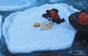
During PIPERS, we deployed 14 WIIOS. Four included the high-resolution Kistler accelerometers (Model A) and ten were the standard WIIOS (Model B). To capture both small-wave and large-wave attenuation, we deployed three WIIOS within or near the MIZ and one further south to ensure we capture the full attenuation of any large-wave events. The Model A WIIOS were deployed furthest south where the wave signal was expected to be smallest. Each WIIOS was deployed on the centre of an ice floe via slip line, zodiac, crane or man basket (Fig. 1). When possible, the thickness of the floes the WIIOS were deployed on was measured using an ice auger. When the WIIOS were deployed by slip line or crane, the ice thickness was determined by visual estimate. Ship-based sea-ice observations collected using the SCAR Antarctic Sea Ice Processes and Climate (ASPeCt) protocol (ASPeCt, 2017) are used to describe the ice conditions between deployments (Appendix B). Note that these ship-based observations are qualitative only and have limitations: the classification of ice conditions may vary between observers and the concentration estimate is made according to the field of view, which is typically only a few kilometres.

Fig. 1. An image taken from the R/V Nathaniel B. Palmer of the deployment of WIIOS B21 at 03:50 on 21 April 2017 at 69.1715833S and 171.8200167E.
Upon entering the ice, four WIIOS were deployed on the sea ice along a meridional transect line on 21 and 22 April 2017 (Fig. 2). The buoys were deployed over ~100 km. The first three (B21–B23) were deployed on pancake ice (<10 m diameter and <0.4 m thick). The ice concentration surrounding each deployment was high (> 90%) and consisted primarily of pancakes, with gaps generally filled with frazil or brash ice. A31 was deployed on continuous thin ice (0.4 m thick) (Appendix Fig. 20). The WIIOS were deployed during a lull in wave conditions and no waves were present. The deployment region was generally characterized by thin pancakes. Between WIIOS B21 and B22, the average ice thickness was 0.3 m. Between WIIOS B22 and A31, the average ice thickness was 0.5 m (Appendix Fig. 18 and Table 3).

Fig. 2. An overview of the inbound WIIOS deployments on the 21 and 22 April 2017. The markers represent the deployed location of each WIIOS. The contours show the sea-ice concentration from satellite imagery at the time of deployment (Meier and others, Reference Meier2017).
Prior to leaving the ice, ten WIIOS were deployed over ~500 km along a meridional transect between 30 May and 3 June 2017 (Fig. 3). The first four (A32–A34 and B24) were deployed furthest south in continuous ice, 0.5–0.7 m thick. B25 was deployed on a floe 100 m wide and 0.6 m thick. The remaining five WIIOS (B26–B30) were deployed on ice floes 20–40 m wide and 0.3–0.75 m thick (Appendix Fig. 21). Ice cores were taken during the deployment of WIIOS A32–A34, B25, B26 and B28. Generally, the ice concentration observed under the ASPeCt protocol during each deployment was high; only on one occasion (during deployment of B27) did it drop below 90%. Small waves were observed from the bridge for about an hour during the deployment of B24. B24 returned waves with 0.2 m significant wave height (H s) and 16 s peak period (T p) during deployment. Waves were also observed from the bridge for the deployments of WIIOS B26–B30. The WIIOS returned the following: B26 returned 0.1 m H s (the minimum limit of the WIIOS) and 17 s T p during deployment, B27 returned 0.1 m H s and 16 s T p 9.5 h after deployment, B28 returned 0.5 m H s and 16 s T p 5 h after deployment, B29 returned 0.6 m H s and 15 s T p 2 h after deployment, and B30 returned 0.7 m H s and 14 s T p 0.5 h after deployment. Generally, the ice floes over the deployment region were young grey-white ice (0.15–0.3 m thick) or first-year ice (0.3–0.7 m thick). Floe sizes over the southern half of the deployment region were generally medium to large (100–2000 m). Over the northern half of the deployment region, the floes were generally smaller (<100 m wide). The ice floes generally decreased in diameter with distance to north, and the floe thickness throughout the region varied between 0.15 and 0.75 m (Appendix Fig. 19 and Table 4)

Fig. 3. An overview of the outbound WIIOS deployments between 30 May and 3 June 2017. The markers represent the deployed location of each WIIOS. The contours show the sea-ice concentration from satellite imagery at the time of deployment (Meier and others, Reference Meier2017).
Results
Overview
In total, we captured 23 466 wave records over 3 months (21 April 2017–26 July 2017). In total, 7297 were captured by WIIOS deployed on the way into the sea ice (inbound) and 16 169 by WIIOS deployed on the way out of the sea ice (outbound). Unfortunately, WIIOS A32's GPS failed prior to deployment so we have not included its records within this dataset. Otherwise, the quality of the records was excellent, with only 123 records being rejected (based on our returned data quality flags). In total, 99.5% of IMU acceleration errors were <20% per record (i.e. <20% unchanged consecutive data or spikes). All of the Kistler records passed quality control and had <20% of errors per record.
WIIOS B22 from the inbound experiment survived the longest (from 21 April to 7 July) and WIIOS A31 from the inbound experiment survived the shortest length (from 22 April to 26 April) (Fig. 4).

Fig. 4. (a) The maximum significant wave height (m) across all WIIOS over time (UTC). (b) A timeline of when each WIIOS was deployed and transmitting wave data.
During the inbound experiment, the WIIOS generally drifted north-west. The sea ice grew in extent faster than the WIIOS drifted north and nearly 40% of the WIIOS wave records were measured at distances 400–500 km from the ice edge (Figs 5a, 6 and 7a). During the outbound experiment, the WIIOS initially drifted north-west. From 15 June 2017, they started to drift towards the east, presumably caught by the Ross gyre and/or strong westerly winds associated with a positive phase of the Southern Annular Mode and were within 150 km of the ice edge the majority of the time. Initially, the WIIOS were deployed in 80–100% ice concentration and spread meridionally. By the end of June, the southern WIIOS had drifted north and the WIIOS were spread zonally. The WIIOS predominately remained close or within the MIZ as they drifted east (Fig. 5b, Figs 8 and 9a). An analysis of the ERA5 reanalysis wind data (not shown here) indicates that the wind and buoy drift velocities time series are highly correlated, with Pearson correlation coefficient r > 0.7 for all buoys, suggesting the observed drift of the buoys is mainly caused by wind-induced stresses. For both the inbound and outbound experiments, the mean sea-ice concentration was >90% (Figs 7b and 9b). Note that the ice edge and MIZ is defined in this analysis by finding the maximum and minimum longitudes from the WIIOS for each sampling period. For each longitude in the range, the latitude is found where the ice concentration is first >15% (ice edge) and first >80% (MIZ southern boundary). We then average across the longitudes to find the mean ice edge and MIZ width at each time step. The distance from the ice edge of each sensor is calculated using only the sensor's latitude. This provides a lower bound estimate on the distance we assume the wave has travelled from the ice edge.

Fig. 5. (a) An estimation of the marginal ice zone width (blue) and the meridional spread of the WIIOS (red) during the inbound experiment. (b) An estimation of the marginal ice zone width (blue) and the meridional spread of the WIIOS (red) during the outbound experiment.

Fig. 6. The evolution of sea-ice concentration from satellite imagery (Meier and others, Reference Meier2017) during the inbound experiment. The large markers represent the location of each WIIOS at the time and date indicated for each subplot and the small markers represent the tracks of each WIIOS for the duration of their deployment. Dates shown are in UTC.

Fig. 7. The inbound experiment frequency distributions of (a) the distance each WIIOS is from the ice edge (km), (b) the mean concentration between WIIOS (%), (c) the significant wave height (H s; m) and (d) the peak period (T p; s).

Fig. 8. The evolution of sea-ice concentration from satellite imagery (Meier and others, Reference Meier2017) during the outbound experiment. The large markers represent the location of each WIIOS at the time and date indicated for each subplot and the small markers represent the tracks of each WIIOS for the duration of their deployment. Dates shown are in UTC.

Fig. 9. The outbound experiment frequency distributions of (a) the distance each WIIOS is from the ice edge (km), (b) the mean concentration between WIIOS (%), (c) the significant wave height (H s; m) and (d) the peak period (T p; s).
Overall, the majority of data collected had significant wave heights of <1 m and peak wave periods between 12 and 16 s (Figs 7 and 9). Note that the data presented in these figures exclude significant wave heights <0.1 m as the peak periods returned for very small waves are falsely too long due to the small signal to noise ratio. In the rest of the analysis, however, we include these data as no waves (or very small waves) remain a valuable data point. We show an example of data collected during one of these small wave events (Fig. 10). This event occurred shortly after deployment while the WIIOS were still spread meridionally. The significant wave height is calculated from the spectral moments and represents four times the std dev. of the surface elevation. The spectra show an increase of the peak wave period (the wave period corresponding to the maximum wave energy) with distance into the ice. We also captured a number of large-wave events (4 records with significant wave heights >9 m, 14 records with significant wave heights between 8 and 9 m and 42 records with significant wave heights between 7 and 8 m). For each of these events, we had multiple WIIOS simultaneously returning wave records (Fig. 4). We show an example of data collected during a wave event while the WIIOS are still meridionally spread (Fig. 11) and a larger wave event with more zonal spread between the WIIOS (Fig. 12).

Fig. 10. A calm wave event on 4 June 2017 at 13:00. (a) A map showing WIIOS locations (coloured markers) and ice concentration (contoured). (b) The significant wave heights leading up to and after the calm wave event. The markers highlight the event at 13:00 on 4 June 2017. (c) Wave spectra from each WIIOS averaged over 1 h.

Fig. 11. A wave event on 6 June 2017 at 22:00. (a) A map showing WIIOS locations (coloured markers) and ice concentration (contoured). (b) The significant wave heights leading up to and after the calm wave event. The markers highlight the event at 22:00 on 6 June 2017. (c) Wave spectra from each WIIOS averaged over 1 h.

Fig. 12. A wave event on 15 June 2017 at 05:00. (a) A map showing WIIOS locations (coloured markers) and ice concentration (contoured). (b) The significant wave heights leading up to and after the calm wave event. The markers highlight the event at 05:00 on 15 June 2017. (c) Wave spectra from each WIIOS averaged over 1 h.
Analysis
We calculate the attenuation of total wave energy by considering the decay rate of significant wave height over distance, i.e. dH s/dx, where H s is the significant wave height and x is distance in metres (Kohout and others, Reference Kohout, Williams, Dean and Meylan2014). Exponential decay of total wave energy with distance is represented by a linear relationship between dH s/dx and H s. Following the method presented in Kohout and others (Reference Kohout, Williams, Dean and Meylan2014), we assume that the wave field is consistent along the zonal spread of the sensors and that as waves enter the sea ice they refract and travel meridionally south. We define the distance between each pair of WIIOS as the difference in latitude. We also assume that for each record, the wave climate persisted long enough to ensure that the wave spectra captured deep within the ice pack is from the wavefront captured near the ice edge. We calculate the decay for each adjoining pair of sensors and present this using a box plot as it is non-parametric and its characterization of the distribution is resilient to outliers. The northernmost sensor determines which significant wave height bin the data point fits into. Each bin is sorted and the median, 25th percentile and 75th percentile are calculated. Note that in the analysis that follows, we remove all data exhibiting wave growth (4049 records or 17%).
We first consider a comparison between the SIPEX-II and the PIPERS datasets (Fig. 13 and Appendix B). Beyond 100 km from the ice edge (Fig. 13a), we see a sudden reduction in decay rates for significant wave heights >4 m in the PIPERS dataset. The PIPERS data do not indicate constant decay for large waves as was seen in the SIPEX-II data (Kohout and others, Reference Kohout, Williams, Dean and Meylan2014). We see a linear relationship between H s and decay rate in the SIPEX data when we consider waves within 100 km of the ice edge (Fig. 13b). We also see a linear relationship in the PIPERS data, but there are two distinct decay rates, with a faster decay rate for waves larger than 5 m. Also note the large decay rates for waves closest to the ice edge relative to waves beyond 100 km from the ice edge.

Fig. 13. A comparison of the significant wave height (H s) decay rates from SIPEX-II (Kohout and others, Reference Kohout, Williams, Dean and Meylan2014) (green circles) and PIPERS (blue squares). (a) Data from WIIOS beyond 100 km from the ice edge. (b) Data from WIIOS within 100 km from the ice edge. Data are binned in 1 m boxes. The markers are the median within each box. The shaded boxes show the range within which 50% of the data lie. The number of data points within each box is displayed above/below the box.
Using the NOAA/NSIDC Climate Data Record of Passive Microwave Sea Ice Concentration, Version 3 (Meier and others, Reference Meier2017), we consider the effect of ice concentration on the wave decay. To avoid coincidental dependence on H s, since high T p is related to high H s, we separate the data into two categories: peak periods >14 s and peak periods <14 s. We then compare the decay rates between the WIIOS in ice concentrations >80% relative to the WIIOS in ice concentrations <80% (Fig. 14). We approximate the ice concentration for each pair of WIIOS by finding all the ice concentration grid points within the region between the WIIOS and averaging. The region between the WIIOS is defined by the minimum/maximum north, south, east and west locations of the two WIIOS. For both short and long periods, the data suggest a linear relationship between H s and decay rate for ice concentrations <80%. For ice concentrations >80%, we see faster decay rates for H s >2 m. For short peak wave periods, there is a linear relationship. For long peak wave periods, there is also a linear relationship, but there are again two distinct decay rates; with a faster decay rate for waves larger than 5 m. The differences in magnitude and slope of decay rates in high concentration ice (>80%) vs low concentration ice (<80%) (Fig. 13) highlight the importance of considering sea-ice concentration when analysing wave-ice data. Sea-ice thickness observations were made from the ship until 5 June, and during this period, they varied between 15 and 75 cm, and we assume ice thickness would also be highly relevant when analysing wave-ice data.

Fig. 14. Decay rates of WIIOS in ice concentrations <80% (blue squares) and WIIOS in ice concentrations >80% (green circles). (a) Data from WIIOS with peak periods <14 s. (b) Data from WIIOS with peak periods >14 s. Data are binned in 1 m boxes. The markers are the median within each box. The shaded boxes show the range within which 50% of the data lie. The number of data points within each box is displayed above/below the box. The black lines show the least-squares regression line of best fit to the median values within each box.
The empirical model derived from Figure 14 is

where x is distance (m) and IC is ice concentration (%).
We also consider the impact of considering wave direction when calculating the wave attenuation between the WIIOS. As the WIIOS did not return wave direction, we consider a global implementation of the WAVEWATCH III (v4.18) third-generation spectral wave model, forced by ERA-Interim input fields (Gorman and Oliver, Reference Gorman and Oliver2018). Generally, this model estimated north westerly swells at a fixed position (65°S,183°E) just beyond the ice edge for the duration of our experiment, with the most frequent direction 300° true north (Fig. 15a). The WIIOS were oriented close to this incident wave direction, between 270 and 315°, 33% of the time (Fig. 15b). To estimate the wave attenuation, we assume that the wave field is consistent along the zonal spread of the sensors. We remove data where the northernmost WIIOS is east of the southernmost WIIOS. We ignore the longitude distance between the WIIOS and assume the angle between each WIIOS pair is 300°. Using basic trigonometry, we can then calculate an artificial distance between the buoys using the difference in latitude. Using this method, the data exhibiting wave growth was 2526 or 11%. The empirical model derived from this method is


Fig. 15. (a) Frequency distributions of the daily wave directions at (65°S,183°E) from a global implementation of the WAVEWATCH III (v4.18) third-generation spectral wave model, forced by ERA-Interim input fields (Gorman and Oliver, Reference Gorman and Oliver2018). (b) Frequency distributions of the zonal angle between each WIIOS pair.
We see that this method alters the attenuation coefficients and significantly reduces the noise in the dataset (Fig. 16).

Fig. 16. Decay rates of WIIOS with wave direction approximations in ice concentrations <80% (blue squares) and WIIOS in ice concentrations >80% (green circles). (a) Data from WIIOS with peak periods <14 s. (b) Data from WIIOS with peak periods >14 s. Data are binned in 1 m boxes. The markers are the median within each box. The shaded boxes show the range within which 50% of the data lie. The number of data points within each box is displayed above/below the box. The black lines show the least-squares regression line of best fit to the median values within each box.
We are now ready to compare the PIPERS empirical model with previous wave-ice empirical and parametric studies. Typically, wave ice attenuation (α) is expressed in terms of wave energy (E)

where x is distance (m), which gives

Assuming linear wave theory

where H is wave height. This gives

which gives

Note that α is frequency-dependent as the ice cover acts as a low-pass filter, so that high-frequency waves are diminished rapidly relative to low-frequency waves. Since α is non-constant, a component-by-component exponential attenuation does not yield a constant exponential attenuation of H s and complicates the relationship between H s and its slope. Nevertheless, the above relationship is a useful approximation to enable a comparison between the empirical model presented here and previous studies using α. We consider the empirical and parametric forms for the attenuation of waves in sea ice implemented into WAVEWATCH III (WW3DG; Collins and Rogers, Reference Collins and Rogers2017). Parametrizations designed for the Arctic include an exponential fit to the field data of Wadhams and others (Reference Wadhams, Squire, Goodman, Cowan and Moore1988) (IC4M1), a quadratic fit to the calculations of Kohout and Meylan (Reference Kohout and Meylan2008) given in Horvat and Tziperman (Reference Horvat and Tziperman2015) (IC4M3) with ice thickness = 0.5 m, and a simple step function with up to 4 steps (may be non-stationary and non-uniform) (IC4M5). For the Antarctic, we consider a polynomial fit in Meylan and others (Reference Meylan, Bennetts and Kohout2014) (IC4M2), Eqn (1) of Kohout and others (Reference Kohout, Williams, Dean and Meylan2014) (IC4M4) and a formula from Doble and others (Reference Doble, Carolis, Meylan, Bidlot and Wadhams2015) with ice thickness = 0.5 m (IC4M7). We also consider an empirical model from a storm event in the Beaufort sea (Montiel and others, Reference Montiel, Squire, Doble, Thomson and Wadhams2018) (Fig. 17). The attenuation coefficients we generate from the PIPERS dataset are comparable to the majority of previous findings. The attenuation coefficients from ICM3 and ICM5 are comparably high for high-frequency waves, but this may be altered depending on the ice thickness variable.

Fig. 17. The various empirical or parametric forms for the attenuation of waves in sea ice used in WAVEWATCH III (REF) compared to an analysis of a storm event in the Beaufort Sea marginal ice zone (REF) and the PIPERS dataset including the wave direction approximation. Attenuation coefficients from both the Antarctic (purple) and Arctic (red) are shown. The shaded regions show the range of attenuation coefficients across all significant wave heights.
Summary
Fourteen WIIOS were deployed on Antarctic sea ice during the PIPERS expedition in autumn 2017. The WIIOS were deployed during the inbound and outbound legs of the cruise. This paper describes the WIIOS and the returned dataset.
The sea ice throughout the experiments generally consisted of pancake and young thin ice (<70 cm). The four WIIOS deployed during the inbound experiment were deployed in the MIZ and remained within the MIZ for ~2 weeks. No major wave events were captured during this inbound experiment. Ten WIIOS were deployed during the outbound experiment, and generally remained within the MIZ for the duration of the experiment. Several large-wave events were captured, with the largest recorded wave over 9 m.
We give an overview of the data returned from the WIIOS and study the attenuation rate of the total wave energy during the PIPERS experiment. The large dataset is broken into long and short peak wave periods and high and low ice concentrations, showing that generally during this experiment, the total wave energy decayed exponentially through the ice with the rate of decay dependent on ice concentration. These results suggest that the conclusion in Kohout and others (Reference Kohout, Williams, Dean and Meylan2014), that large waves decay linearly, is an artefact of analysing a small dataset in different ice conditions. For example, it is possible that during SIPEX-II, the large-wave events predominantly occurred when low ice concentrations were present, thereby reducing the decay rates and leading to an appearance of linear wave decay. The PIPERS dataset is relatively a very large dataset and more analysis is required to understand the complex interaction of waves with ice thickness and concentration and how this is reflected through the attenuation of wave energy.
Supplementary material
The supplementary material for this article can be found at https://doi.org/10.1017/aog.2020.36
Acknowledgements
We thank Steve Ackley and the captain and crew of RV Nathaniel B. Palmer for their assistance in deploying the waves-in-ice instruments. We also thank Erick Rogers for his contribution and feedback, Lily Gamson for analysing the ERA5 reanalysis wind data and Richard Gorman for providing the WAVEWATCH III (v4.18) third-generation spectral wave model results. The work was funded through New Zealand's Deep South National Science Challenge Targeted Observation and Process-Informed Modelling of Antarctic Sea Ice, NIWA core funding under the National Climate Centre Climate Systems programme, the Australian Research Council Discovery Project ‘Investigating the impact of enhanced Southern Ocean wave penetration on Antarctic sea ice with robots from above, below and within’, and the Marsden Fund project ‘Breaking the ice: process-informed modelling of sea-ice erosion due to ocean wave interactions’ (18-UOO-216) administered by the Royal Society of New Zealand.


 Open access