


Introduction
Many key questions in political science have a temporal dimension, including set-relational questions that focus on necessary and/or sufficient conditions or combinations of conditions (configurations) (Schneider and Wagemann, Reference Schneider and Wagemann2012). A researcher may ask: is there (a lack of) stability in the necessary or sufficient conditions or configurations for strong economic performance (Vis et al., Reference Vis, Woldendorp and Keman2013)? Or: how do the configurations that are sufficient for party position change (see Fagerholm, Reference Fagerholm2016), or for public policy reform (see Fischer and Maggetti, Reference Fischer and Maggetti2017), change over time? Given the relevance of time (e.g. Aminzade, Reference Aminzade1992; Abbott, Reference Abbott2001; Pierson, Reference Pierson2004), it is not surprising that political scientists’ methodological toolkit by now includes numerous methods and techniques that put time at center stage. The toolkit includes quantitative methods and techniques, like (pooled) time series analysis (e.g. Beck and Katz, Reference Beck and Katz1995; Baltagi, Reference Baltagi2005), survival analysis (Hosmer et al., Reference Hosmer, Stanley and May2008), and event history modeling (e.g. Box-Steffensmeier and Jones, Reference Box-Steffensmeier and Jones2004). It also includes qualitative ones, such as process tracing (George and Bennett, Reference George and Bennett2005; Bennett and Checkel, Reference Bennett and Checkel2014) and sequence analysis (Mahoney et al., Reference Mahoney, Kimball and Koivu2009).
All these methods and techniques have their merits, but what they cannot do for a medium-to-large set of cases is tracking configurations over time – which is what is needed to answer the questions above. We, therefore, focus on an approach that can track configurations over time for a (much) larger set of cases than could a small-n qualitative approach such as process tracing, namely: Qualitative Comparative Analysis (QCA).
QCA is a configurational research approach that uses set-theory and formal logic, and Boolean and fuzzy-set algebra, to calibrate conditions and analyze truth tables, to identify necessary and/or sufficient conditions – or combinations of conditions, that is configurations – for an outcome (Berg-Schlosser et al., Reference Berg-Schlosser, De Meur, Rihoux, Ragin, Rihoux and Ragin2009; Schneider and Wagemann, Reference Schneider and Wagemann2012). QCA allows for equifinality and multifinality (Rihoux and Ragin, Reference Rihoux and Ragin2009; Schneider and Wagemann, Reference Schneider and Wagemann2012). Equifinality means that there may be multiple configurations that produce the same outcome. Multifinality means that depending on the configuration it is in, a condition may contribute to producing both the outcome (Y) and its negation (~Y). These phenomena are relevant for many questions in political science, which helps to explain the extensive use of QCA in the field.Footnote 1
Even though QCA itself is insensitive to time (e.g. Byrne and Callaghan, Reference Byrne and Callaghan2014), several authors have provided overviews of strategies to address time in QCA (see Schneider and Wagemann, Reference Schneider and Wagemann2012: 263ff; Fischer and Maggetti, Reference Fischer and Maggetti2017; Gerrits and Verweij, Reference Gerrits and Verweij2018: 120–33). These overviews, however, neither focus specifically on strategies to track configurations over time, nor do they include empirical demonstrations of the strategies. Our contribution is to demonstrate and discuss QCA-related strategies to track configurations over time and to highlight their differences. We assume that readers have basic knowledge of QCA; we refer those readers who don’t to available textbooks (Ragin, Reference Ragin1987, Reference Ragin2000, Reference Ragin2008; Rihoux and Ragin, Reference Rihoux and Ragin2009; Schneider and Wagemann, Reference Schneider and Wagemann2012).
We examine three strategies to track configurations over time: Multiple Time Periods, Single QCA (Strategy A); Multiple QCAs, Different Time Periods (Strategy B); and Fuzzy-Set Ideal Type Analysis (Strategy C). In each strategy, the researcher first segments the cases into different time points or periods. A case here is understood as a socio-spatial unit (e.g. country, government) that is studied on a number of explanatory conditions (e.g. economic growth and unemployment level; see Vis, Reference Vis2011) and an outcome of interest (e.g. labor market policy; see Vis, Reference Vis2011). The socio-spatial unit is segmented in different time points, creating multiple cases for a single socio-spatial unit. Strategy A includes all cases in one QCA, focusing on tracking solution terms (i.e. configurations) over time. Strategy B involves running different QCA’s for cases belonging to the same time period, focusing on tracking solution formulas (i.e. strings of configurations) over time. These first two strategies extend the full QCA research process by amending the comparative analysis of configurations. Strategy C focusses on tracking cases over time, tracing how a single socio-spatial unit develops over time. This strategy only addresses the fuzzy-set and calibration part of the QCA research approach. In the first two strategies, the focus is on the configurational solution terms or formulas (explanatory approach) and in the third strategy, the focus is on the cases-as-configurations (descriptive approach).
To date, not many studies aim to track configurations over time. Yet, doing so opens up a whole range of novel research directions. Let us take two recent studies from this journal as an example. The first is Haesebrouck and Van Immerseel’s (Reference Haesebrouck and van Immerseel2020) study on what explains the variation in the degree of contestation in parliament for military deployment. Their 69 cases are military deployments between 1991 and 2016, thus having a temporal dimension. Although Haesebrouck and Van Immerseel (Reference Haesebrouck and van Immerseel2020) do not focus on this dimension, their results can easily be grouped into a few time periods (cf. Table 1 below), enabling examining whether the configurations that are sufficient for high levels of political contestation remain (or change) over time. This would be an example of our Strategy A: ‘Multiple Time Periods, Single QCA’. The second example is Casal Bértoa and Rama’s (Reference Casal Bértoa and Rama2020) analysis of the rise in electoral support for anti-political-establishment parties between 1849 and 2017 in 20 countries. Casal Bértoa and Rama (Reference Casal Bértoa and Rama2020) are interested in the correlation of economic, institutional, and sociological change factors and support for anti-political-establishment parties. But if they would calibrate their data into crisp or fuzzy sets, the data would also allow for a research question on tracking configurations over time: are the conditions or configurations necessary and/or sufficient for support for such parties stable over time? In this case, both Strategy A and Strategy B: ‘Multiple QCAs, Different Time Periods’ would be possible. For Strategy A, the crisp-set or fuzzy-set data could be used as-is; for Strategy B, the crisp-set or fuzzy-set data would need to be split up into meaningful time periods.
Table 1 Multiple time periods, single QCA (Strategy A), extension of Vis (Reference Vis2011), conservative solution
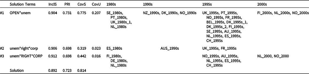
‘InclS’ is the consistency score of the solution terms, ‘PRI’ is the Proportional Reduction in Inconsistency, ‘CovS’ is the raw coverage score of the solution terms, and ‘CovU’ is the unique coverage score of the solution terms.
Of course, it depends on the specific topic of whether a research question that focuses on tracking configurations over time is relevant. Our point is to show three different strategies that researchers have at their disposal in case they want to track configurations over time.
Before we explain and demonstrate the three strategies, we first review existing literature on time and QCA in Sect. 2. We conclude from this review that only one strategy presented in that literature so far is suitable for tracking configurations over time. We discuss this strategy, and two other ones that we identified, in Sect. 3–5. The three strategies are compared in Sect. 6. Conclusions are drawn in Sect. 7.
Time and QCA
Thus far, QCA applications are typically cross-sectional and time-insensitive and this lack of attention to time is considered the main limitation of QCA (De Meur et al., Reference De Meur, Rihoux, Yamasaki, Rihoux and Ragin2009). Griffin (Reference Griffin1992), for example, argued that QCA sees time as temporal context, with explanations ensuing from its application having ‘nothing intrinsically to do with sequential unfolding, or historical movement through time’ (Reference Griffin1992: 412). Relatedly, Boswell and Brown (Reference Boswell and Brown1999) recognized that QCA indeed allows for the comparison of ‘whole cases’ but with the consequence of ‘static comparison that is not fully compensated by the use of temporally contingent determinants’ (Boswell and Brown, Reference Boswell and Brown1999: 181).
Approach to QCA and concept of time
Let us first clarify our approach to QCA, which affects how tracking configurations can be understood. This article follows a ‘realist’ (Schneider, Reference Schneider2018) or ‘substantive interpretability’ (Thomann, Reference Thomann, Peters and Fontaine2020; Thomann and Maggetti, Reference Thomann and Maggetti2020) approach to explanation in QCA. A basic premise is that social reality is deeply complex; certain conditions or configurations can trigger, under certain circumstances, mechanisms that cause events or phenomena, that is outcomes of interest (Gerrits and Verweij, Reference Gerrits and Verweij2013; Gerrits and Pagliarin, Reference Gerrits and Pagliarin2020). The idea is that QCA can be deployed to identify and analyze meaningful and plausible explanatory configurations (Thomann and Maggetti, Reference Thomann and Maggetti2020). This is the approach to QCA that is most widespread in practical social science research (Thomann, Reference Thomann, Peters and Fontaine2020). Tracking configurations, then, concerns identifying the development of configurations over time, to allow the researcher to identify how a certain outcome of interest may be explained differently at different times.
The notion of trajectory shows affinity with the concept of configuration. Aminzade (Reference Aminzade1992: 462) uses the term ‘paths’ as a synonym for ‘trajectories’; the term ‘paths’ has become nomenclature in the QCA literature to refer to the multiple solution terms or minimized configurations that are sufficient for an outcome (e.g. Rihoux and Ragin, Reference Rihoux and Ragin2009; Schneider and Wagemann, Reference Schneider and Wagemann2012). Clearly, however, ‘paths’ in terms of trajectories are temporal processes, whereas in QCA they typically refer to static configurations. Still, scholars have highlighted the resemblance between trajectories and configurations. Aminzade observed that ‘in studying the temporal intersection of different trajectories, sociologists have often emphasized the way in which this intersection produces key moments, or conjunctures that mark the coming together of relatively autonomous processes’ (Reference Aminzade1992: 467). Aminzade observed that the overlapping or intersecting of multiple trajectories creates points in time or events that may lead to certain outcomes. Byrne (Reference Byrne2005, Reference Byrne, Byrne and Ragin2009) also refers to the resemblance between trajectories and configurations, though in a subtly different manner. He views cases-as-complex-systems as configurations and considers that ‘the trajectories of systems are the histories of cases’ (Reference Byrne2005: 105) or the ‘path through time of a system’ (Reference Byrne, Byrne and Ragin2009: 104). Using Ragin’s (Reference Ragin1987) method, the Boolean truth tables are ‘representing specific configurations which have engendered particular trajectories towards an outcome’ (Byrne, Reference Byrne2005: 106). He adds the idea that Ragin’s (Reference Ragin2000) fuzzy-set QCA, in particular the cross-over point that distinguishes cases that are different-in-kind, may be used to think about the thresholds that indicate when a system undergoes a ‘phase shift’ (Byrne, Reference Byrne2005: 107, Reference Byrne, Byrne and Ragin2009: 109) or system change.
In both Aminzade and Byrne’s conceptualizations, trajectories and configurations are somehow consecutive. Their approaches are not concerned with the tracking of configurations over time per se. In this article, we view trajectory as the development of solution terms (Strategy A), solution formulas (Strategy B), or cases (Strategy C) over time. The solution terms, in turn, are represented by cases that are defined as configurations, that is combinations of conditions. Comparative methods have mainly focused on drawing conclusions about patterns across cases or the world in general, instead of about the trajectories of configurational cases (Bevan, Reference Bevan, Byrne and Ragin2009). The latter is what we intend to contribute to in this article.
Strategies from the existing literature to include time in QCA
As several authors have explained and demonstrated, QCA can be made more time-sensitive by conducting a mixed-methods study, in which a static QCA is followed by a qualitative or quantitative approach that is sensitive to time. A researcher can, for instance, first conduct a QCA and subsequently apply process tracing (see Schneider and Rohlfing, Reference Schneider and Rohlfing2016; Beach and Rohlfing, Reference Beach and Rohlfing2018). The researcher then examines the temporal dimension – specifically the process linking the configuration to the outcome – in the second stage. However, process tracing is necessarily limited to a select number of cases and is not focused on tracking configurations over time – the focus of the present article. A quantitative approach, like time series analysis, is applicable to a large set of cases. However, like process tracing, time series analysis is unsuited for tracking configurations over time. Moreover, the high number of cases that are required for time series analysis may be problematic for many questions QCA researchers are interested in. In addition to a mixed-methods approach, where QCA is combined with another method to make it more time-sensitive, strategies have also been proposed that seek to integrate time in the method itself.
Focusing on public policy analysis, Fischer and Maggetti (Reference Fischer and Maggetti2017) list five strategies to include time in QCA. The first strategy is the use of time-related conditions (p. 354, see also Schneider and Wagemann, Reference Schneider and Wagemann2012: 266). Examples include constructing a set of ‘old’ (or ‘young’) units of analysis or a set of ‘quick’ (or ‘slow’) ones. It is also possible to include a temporal order in the condition (e.g. ‘strong economic performance following democratization’). An advantage of this strategy is that it is simple and widely applicable; disadvantages are that it only indirectly incorporates time and that the adding of conditions increases the problem of limited diversity (Fischer and Maggetti, Reference Fischer and Maggetti2017). Another disadvantage is that just including one or more time-related conditions in what is otherwise a static QCA does not enable a researcher to track configurations over time.
The second strategy Fischer and Maggetti (Reference Fischer and Maggetti2017) list is the aggregate operationalization of procedural variables. The idea here is:
(…) to aggregate quantities that vary over time to incorporate a procedural element into calibrated conditions. For instance, (…) to account for the participation of an actor in the course of a given policy-making process, we could proceed as follows. First, we have to break the process in a number of discrete events, which are not necessarily sequential, such as (1) agenda setting; (2) explorations; (…); (8) sanctioning/evaluation. Then we can observe the participation of the target actor in each one of these events, and finally aggregate the obtained scores in a single condition to be included in the QCA analysis (Fischer and Maggetti, Reference Fischer and Maggetti2017: 355).
While we see the benefit of this strategy for analyzing political processes, it may not be widely applicable because many processes cannot be broken up into a number of discrete events. Regardless, the strategy does not allow a researcher to track configurations over time.
The third strategy Fischer and Maggetti (Reference Fischer and Maggetti2017: 356) mention, as do Schneider and Wagemann (Reference Schneider and Wagemann2012: 266), is to make temporal use of two-step QCA (Schneider and Wagemann, Reference Schneider and Wagemann2006; see Schneider, Reference Schneider2019 for a recent reconceptualization). There, the first part of the analysis of the remote conditions includes conditions that are remote in time. The analysis’s second part then includes the more proximate conditions immediately triggering an outcome. While the different conditions included in the two-step QCA vary in the degree to which they are temporally close to the outcome, the analysis itself remains cross-sectional. The strategy does not involve the tracking of configurations over time.
The fourth strategy they discuss is the comparison of separate analyses for each point in time, which is also mentioned by Schneider and Wagemann (Reference Schneider and Wagemann2012: 265) and which is similar to our Strategy B (‘Multiple QCAs, Different Time Periods’). This strategy is particularly apt for tracking configurations over time; we return to it in Sect. 4.
Fischer and Maggetti’s (Reference Fischer and Maggetti2017: 355) fifth strategy is the inclusion of noncommutative sequences of conditions. This is the approach taken in Temporal Qualitative Comparative Analysis (TQCA). TQCA is developed to incorporate time by exploring the causal relevance of sequences of events (Caren and Panofsky, Reference Caren and Panofsky2005). In their much-debated article on TQCA,Footnote 2 Caren and Panofsky (Reference Caren and Panofsky2005; updated by Ragin and Strand, Reference Ragin and Strand2008) add a temporal perspective to QCA by abandoning QCA’s commutativity rule – which is what Fischer and Maggetti (Reference Fischer and Maggetti2017) call the inclusion of noncommutative sequences of conditions.Footnote 3 The commutativity rule states that ‘the order in which two or more sets are connected through Logical-AND and Logical-OR is irrelevant’ (Schneider and Wagemann, Reference Schneider and Wagemann2012: 323). Caren and Panofsky (Reference Caren and Panofsky2005) introduced an operator they labelled THEN to examine whether it is, say, A before B that leads to an outcome. To use this THEN operator, two requirements should be met (Caren and Panofsky, Reference Caren and Panofsky2005): theory should account for the sequence of occurrence (here: A before B) and the researcher should know the sequence in which the conditions occurred empirically in the cases. Obviously, these are important requirements that must be considered when constructing the cases and collecting data. The larger the number of cases and the less in-depth the data generation process, the harder it will be to meet these requirements.Footnote 4 TQCA does not allow a researcher to track configurations over time, but instead examines the sequence in which an outcome unfolds.
Another strategy presented in the literature is Time-Series Qualitative Comparative Analysis (TS/QCA) (Hino, Reference Hino2009). It uses cross-temporal variations in the data to define and calibrate conditions. Subsequently, the truth table construction and its minimization proceed as normal. There are three variants of TS/QCA: Pooled QCA, Fixed Effects QCA, and Time Differencing QCA (Hino, Reference Hino2009). In Pooled QCA, each case is measured with respect to its conditions and the outcome for different time periods separately. Pooled QCA introduces the cases’ temporal dimensions in the definition and the calibration of the conditions, based on a cluster analysis of time series data (for details of this procedure, see Hino, Reference Hino2009). This means that the focus is not on tracking configurations over time, although it does not disallow it. In Fixed Effects QCA, the cases’ specific contexts and/or properties can be taken into account to assign the membership scores, setting thresholds separately for each socio-spatial unit (Hino, Reference Hino2009: 255). After the application of Fixed Effects QCA, as with Pooled QCA, the calibrated cases are included in a single QCA truth table minimization as normal. A drawback of TS/QCA is that it uses an inductive approach – cluster analysis – mechanically to set calibration thresholds, which may result in calibrated data that deviate from theoretical and/or substantive knowledge. This problem is compounded when the number of cases per socio-spatial unit is relatively small, as is often the case in political science. The third variant is Time Differencing QCA. Here, the researcher assigns values to cases based on an increase or a decrease in a given condition between two or more time periods, by calculating the differences (Δ) between these time periods. This results in a new case: Δ_Case_1. This case is then calibrated and included with other cases (e.g. Δ_Case_2, Δ_Case_3, etc.) in a calibrated data matrix, which is further analyzed as normal. The differences over time within a case are thus made relative. This approach is suitable ‘when the research is interested in an increase or decrease between two definite time points (…)’ (Hino, Reference Hino2009: 257), which means that it is not suitable for tracking configurations over time. In the next section, we discuss and empirically illustrate three strategies for incorporating time in QCA that do allow for tracking configurations over time.
Multiple time periods, single QCA (Strategy A)
We label the first strategy to track configurations over time using QCA ‘Multiple Time Periods, Single QCA’ (Strategy A). This strategy introduces the temporal dimension in the cases’ definitions (De Meur et al., Reference De Meur, Rihoux, Yamasaki, Rihoux and Ragin2009), with time serving as the primary boundary of a case. The cases’ social and spatial delineations are kept constant, but are split up in different time periods (Gerrits and Verweij, Reference Gerrits and Verweij2018). Some examples of this approach are available in the literature (e.g. Vis, Reference Vis2011; Never and Betz, Reference Never and Betz2014). Never and Betz (Reference Never and Betz2014), for instance, analyzed the climate change performance of seven emerging economies looking at four conditions. The countries were split up into two time periods – 2005 and 2010 – resulting in a total of 14 cases. The cases were then included in a single truth table analysis, identifying sufficient configurations for a weak climate change performance. To illustrate this strategy empirically, we replicate a study by Vis (Reference Vis2011).
Original study and dataset
Vis (Reference Vis2011) analyzed which combinations of conditions influenced the increase of spending on active labor market policies – labelled ‘ACTIVATION’ – of 53 governments in the period between 1985 and 2003 (see Table S.A1 in Supplementary Information A for the included cases). These cases’ socio-spatial delineations are kept constant – that is the 18 countries’ governments – but they are split into different time periods. To highlight the cases’ temporal dimension, we indicate in the fourth column in Table S.A1 the cases-in-a-country in the 1980s (‘1980s’), the period 1990–1994 (‘1990s’), the period 1995–1999 (‘1995s’), and the 2000s (‘2000s’).
The analysis of Vis (Reference Vis2011) included five conditions. The change in the level of unemployment in a country (‘UNEM’) and its economic growth (‘GROWTH’) captured a country’s socioeconomic situation. Because political parties’ room to maneuver increases when the economic situation is improving, fiscally as well as politically, Vis (Reference Vis2011) hypothesized an improving economic situation to be a necessary condition for ACTIVATION. However, her test for necessity did not return any necessary conditions.
To examine which conditions were sufficient for ACTIVATION, Vis (Reference Vis2011) examined three other conditions: partisanship (‘RIGHT’), economic openness (‘OPEN’), and corporatism (‘CORP’). She argued that both left partisanship (i.e. the negation of rightist partisanship) and right partisanship (‘RIGHT’) may contribute to ACTIVATION, depending on other conditions. A country’s economic openness (‘OPEN’) was measured as the total trade in current prices, as a percentage of GDP. Like partisanship, also the effects of ‘OPEN’ and the third condition ‘CORP’ were thus expected to depend on other conditions: that is they were hypothesized to be INUS conditions (see Mackie, Reference Mackie1965). The results of her analysis confirmed that ‘RIGHT’, ‘OPEN’, and ‘CORP’ were INUS conditions. Decreasing unemployment was combined with either an open economy (unem*OPEN), a non-corporatist country with a leftwing government (unem*corp*right), or with a corporatist country with a right-wing government (unem*CORP*RIGHT).
Illustration
Before discussing how we extended Vis’s (Reference Vis2011) analysis to track configurations over time, we first indicate the changes we had to make to the original dataset. Vis’s dataset contained seven cases that were calibrated as 0.5, which is problematic because it means that these cases were excluded from the truth table analysis.Footnote 5 Therefore, we recalibrated these seven cases. Supplementary Information A details the recalibration and the recalibrated data matrix.Footnote 6
Using the recalibrated data, we replicated Vis’s results. Table S.B1 in Supplementary Information B presents the truth table and Table 1 presents the results of the truth table analysis, whereby we extend the results by highlighting the cases’ temporal dimension.Footnote 7 Whereas the original study was a cross-sectional analysis of 53 governments, our analysis focuses on cases-in-a-country in different time periods. To highlight the results’ temporal dimension, we sorted the cases according to the periods they represent. Note that this means that cases that are represented by the same configuration in the truth table (e.g. cases FI_2000s, PT_1995s, and SE_1980s from truth table row #18, see Table S.B1) are now placed in separate columns (see Table 1), whereas normally they would have been presented together.
The results presented in Table 1 offer several insights. First, taking the three solution terms together, it can be observed that most cases are from the 1995s. In this specific analysis, this merely is an artifact of the governments included. Nonetheless, inspecting which period includes most cases may be insightful in other studies like those examining successful (or failed) policies or projects. Second, and substantively more relevant for our reanalysis and extension, on the level of a single solution term, it can for instance be observed that minimized configuration #1 (OPEN*unem) was increasingly empirically present up to the 2000s. That is, in the 1980s, decreasing unemployment (‘unem’), combined with an open economy (‘OPEN’), was sufficient for ACTIVATION in four out of the seven cases.Footnote 8 The other countries were characterized by the absence of corporatism combined with leftist governments, or by corporatism combined with rightist governments. In the 1995s, the combination of decreasing unemployment with an open economy (OPEN*unem) had become the most important explanation for ACTIVATION. Third, on the level of a single country, we can trace how different explanations apply over time. We take Portugal, the country with most cases in the dataset (five cases, see Table S.A1), as an example. Portugal’s decreasing unemployment combined with an open economy (OPEN*unem) explained increased spending in the 1980s and 1995s. The other three Portugal cases, for the 1990s and 2000s, are not covered by the results. The inspection of the data matrix and truth table shows that Portugal had very low spending in the 1990s, and that for the 2000s, no clear explanations are available (see the low PRI scores for configurations #22 and #23 in Table S.B1). This may prompt the researcher to explore other explanations for that period. For example, the data indicate that PT_2000s_1 had a leftist government and PT_2000s_2 had a rightist government, which may explain the above findings.
By presenting the different time periods to which the cases covering a solution term (i.e. configuration) belong – as in Table 1 – the researcher is able to map the development of cases in terms of how they are represented by different configurations over time or, conversely, of how different configurations are represented by different cases over time. This means that the strategy ‘Multiple Time Periods, Single QCA’ allows us to track solution terms over time. It can show how certain explanations – as represented by configurations – become less or more relevant in time, or how explanations apply in certain eras or periods and not others. In the next strategy, the focus shifts to tracking the solution formulas over time.
Multiple QCAs, different time periods (Strategy B)
Strategy B is to execute multiple, separate QCAs for the same sample of cases for different time periods. In the Vis (Reference Vis2011) data, this strategy means conducting separate QCAs for the 1980s, 1990s, 1995s, and 2000s. The researcher subsequently inspects the solution formulas for the different time periods (cf. Fischer and Maggetti, Reference Fischer and Maggetti2017). There are various ways to go about here. The simplest is to ‘eyeball’ the solution formula for the different time periods to examine which of the solution terms emerge in each time period, how many and which cases correspond to the solution terms in the time period, and how this changes over time. A more refined way would be to string the solution formulas for the different time periods together, creating a time series of minimized configurations leading to the outcome. This time series reveals both the conditions that remain constant over time and those that change. This latter way is particularly interesting when a researcher aims ‘to find a set of explanatory factors that are stable for a certain period, or, on the contrary, to discriminate between periods that are characterized by different explanatory factors, such as in the case of the identification of critical junctures and path-dependent processes’ (Fischer and Maggetti, Reference Fischer and Maggetti2017: 356).
The strategy Multiple QCAs, Different Time Periods have been applied in empirical research only a few times (e.g. Järvinen et al., Reference Järvinen, Lamberg and Pietinalho2012; Basurto, Reference Basurto2013; Vis et al., Reference Vis, Woldendorp and Keman2013), where solution formulas were produced for two or three time periods and then compared. Especially when stringing the different solution formulas together to examine how minimized configurations change over time, it can be challenging to interpret the results (Gerrits and Verweij, Reference Gerrits and Verweij2018).
Illustration using the Vis (Reference Vis2011) data
To empirically illustrate this strategy, we divided Vis’s (Reference Vis2011) 53 cases-in-a-country into four time periods: ‘1980s’, ‘1990s’, ‘1995s’, and ‘2000s’. While for Strategy A we pooled all the cases from these periods together, for Strategy B we split up the data into four separate data matrices: one for each period. These four data matrices can be derived simply from Table S.A1; they include 14, 15, 16, and 8 cases, respectively. With five conditions, this means that the cases-to-conditions ratio is off for the analyses of the cases from the 1980s and the 2000s and that it is just acceptable for the 1990s and 1995s (Marx, Reference Marx2010). The analyses presented here are therefore only intended to be illustrative for this specific strategy.
The truth tables for the four time periods, including the substantiations of the consistency cut-off points, are included in Tables S.C1 through S.C4 in Supplementary Information C. As expected, with five conditions, the truth tables include quite some logical remainders (not displayed in the tables in Supplementary Information C), leading to rather complex results. Therefore, and again for illustrative purposes only, we continue with the parsimonious results for the four periods, which Table 2 provides. For readability, we report the solution formulas and the covered cases only; the full results are displayed in Tables S.C5 through S.C8 in Supplementary Information C. For the 1990s and the 1995s, more than one model is identified (see Baumgartner and Thiem, Reference Baumgartner and Thiem2017), respectively, four and six (see Tables S.C6 and S.C7). Because our aim here is to illustrate this strategy, we simply picked the model for these periods that has the highest consistency and coverage scores and included those in Table 2. Each cell in the table presents one solution term for a specific time period, with the cases that are covered by the solution term.
Table 2 Multiple QCAs, different time periods (Strategy B), parsimonious solutions
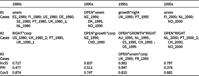
‘InclS’ is the consistency score of the solution terms, ‘PRI’ is the Proportional Reduction in Inconsistency, and ‘CovS’ is the raw coverage score of the solution terms.
Visualization can help to better understand QCA results. Figure 1 therefore visualizes the results. The solution per period can be read from left to right. Black (blank) symbols indicate the presence (absence) of a condition. The symbol’s shape indicates which conditions belong to the same solution term. For example, the solution formula for the 2000s is unem + RIGHT*OPEN. To reveal which conditions are (somewhat) stable over time, we included the blue elongated surfaces. The absence of unemployment (‘unem’) is, for instance, a stable condition across all periods. Growth, either present or absent, conversely, is not. Finally, to reveal which configurations (or subparts thereof) are (somewhat) stable over time, we added the red circular surfaces. For instance, the combination of RIGHT*OPEN, either as a solution term in itself (in the 2000s) or as part of a solution term (in the 1995s), reoccurs over time.

Figure 1. Visualization of the time series of minimized configurations, based on Vis (Reference Vis2011).
The shape of the symbols (circle, square, or triangle) indicates which conditions are part of the same solution term. Black symbols indicate the presence of a condition and blank symbols the negation of a condition. For example, the solution formula for the 1980s is: unem + RIGHT*corp, which is visualized as UNEM[![]() ] + RIGHT[
] + RIGHT[![]() ]*CORP[
]*CORP[![]() ]. The blue elongated surfaces indicate which conditions are (somewhat) stable over time. The red circular surfaces indicate which configurations (or subparts of configurations) are (somewhat) stable over time.
]. The blue elongated surfaces indicate which conditions are (somewhat) stable over time. The red circular surfaces indicate which configurations (or subparts of configurations) are (somewhat) stable over time.
How can we track configurations over time based on the results in Table 2 and Figure 1? To compare the formulas, a researcher can, for example, focus on the first moment or period and the last one, hence taking a longer-term perspective. In both the 1980s and the 2000s, one of the paths toward ACTIVATION was a decreasing level of unemployment (‘unem’), that is an improving socioeconomic situation. The other paths for those time periods are also somewhat similar: in both periods, it is a right-wing government (‘RIGHT’) combined with another condition.
Comparing only these two periods, a researcher might conclude that the changes have been relatively minor. This latter conclusion fails to hold if s/he would also examine the in-between periods of the 1990s and the 1995s. Whereas in the 1980s and the 2000s, a decreasing level of unemployment was an individually sufficient condition, in the 1990s and 1995s, it was ‘only’ an INUS condition.
The analysis also highlights which (combinations of) conditions are stable over time and which change. As indicated by the blue elongated surfaces in Figure 1, many countries with an increase in active spending were characterized by a decreasing level of unemployment through the four periods. Moreover, a low degree of corporatism has characterized the 1980s to the 1995s and high openness has characterized the 1990s to the 2000s; they were INUS conditions for ACTIVATION. The analysis also indicates that from the 1995s onwards, a right-wing government consistently combined with a high openness to explain ACTIVATION, as indicated by the red circular surfaces in Figure 1.
Fuzzy-set ideal type analysis (Strategy C)
Fuzzy-set ideal type analysis is an ideal type analysis that makes use of fuzzy-set theory (see e.g. Kvist, Reference Kvist2007). With two conditions, the multidimensional property space has 22 = four corners: the ideal types. These ideal types correspond to the rows in the truth table. The researcher calculates a case’s membership score to an ideal type by applying the ‘weakest link in the chain’ principle (Schneider and Wagemann, Reference Schneider and Wagemann2012: 44): an ideal type’s membership equals the minimum of the membership scores of the respective conditions. The configuration in which a case has a membership of >0.5 is the ideal type it represents. A case can only represent one ideal type at the same time (Schneider and Wagemann, Reference Schneider and Wagemann2012). When calculating the case’s ideal type for different periods in time, a researcher can analyze how cases move (or not) over time in the property space. Fuzzy-set ideal type analysis is still used relatively scantly in empirical research (see e.g. Kvist, Reference Kvist2007; Vis, Reference Vis2007; Hudson and Kühner, Reference Hudson and Kühner2009; Marchal and Van Mechelen, Reference Marchal and Van Mechelen2017). Yet, since it requires only a truth table and not the full QCA research process, it is a straightforward and promising strategy to track configurations over time. An important difference with the other two strategies is that fuzzy-set ideal type analysis focusses on the case’s conceptualization as a configuration of aspects, whereas the other two strategies place configurations as combinations of conditions in a solution term or formula at the forefront. The descriptive nature of fuzzy-set ideal type analysis makes it suitable for research questions of a more exploratory and case-focused nature, for instance for creating typologies. To illustrate the strategy, we make use of the Vis (Reference Vis2011) dataset as follows.
We develop four ideal types based on two sets. The first set is activation (‘ACTIVATION’), which was the outcome in Strategies A and B. ACTIVATION indicates whether a case’s welfare state is best characterized as active or as passive. We newly add the second set: generosity (‘GEN’), which captures whether a case has a generous benefit system (in the set of GEN) or a lean one (outside the set of GEN). Table 3 displays the property space with the resulting four ideal types: a generous activating welfare state, with high levels of benefit generosity and activation (AG); a generous passive welfare state, with high levels of benefit generosity and little activation (aG); a lean activating welfare state, with low levels of benefit generosity and a high level of activation (Ag); and a lean passive welfare state, with low levels of benefit generosity and little activation (ag). Combining the two sets enables a researcher to examine whether and how the welfare states of our cases – which, as in the first two strategies, are cases-in-a-country in different time periods – change over time. Changes can be quantitative (in degree) – when a case’s membership score to an ideal type increases or decreases over time – or qualitative (in kind) – when a case’s membership score shifts from one ideal type to another.
Table 3 Property space of activation and generosity
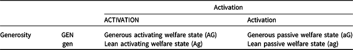
Capital letters indicate the presence of the condition and lowercase letters indicate the absence of the condition.
To measure generosity (‘GEN’), we follow Vis (Reference Vis2007) and use an index of the net replacement rates of unemployment insurance benefits and sick pay from the updated Comparative Welfare Entitlements Dataset (Scruggs et al., Reference Scruggs, Detlef and Kuitto2017). To turn the raw data for GEN into fuzzy sets, we followed Kvist (Reference Kvist2003) and set the first qualitative anchor point (0.0; fully out of the set of GEN) below 0.20 and the second qualitative anchor point (1.0; fully in the set of GEN) at ≥0.90.Footnote 9 The fuzzy scores between 0 and 1 are calculated in line with Vis (Reference Vis2007: 112): we have taken the raw data and subtracted the lower limit (0.20), and then divided the result by the upper limit minus the lower limit, here: 0.90 – 0.20 = 0.70.
Table S.D1 in Supplementary Information D displays the calibrated data matrix for the 53 cases-in-a-country (i.e. the governments) and the fuzzy-set membership scores of each case in each ideal type. Table 4 displays what we label an ‘adjusted truth table’ that was created using R (Duşa, Reference Duşa2018, Reference Duşa2019). The table is not a traditional truth table, because an outcome (Y or ~Y) plays no role. However, it does provide a succinct overview of which cases belong to which of the four ideal types. Table 4 can be used to assess a case’s changes. Looking into qualitative changes, we see that Portugal – highlighted in bold in Table 4 – moved from the ideal type AG in the 1980s to aG in the 1990s, and back again to the first ideal type in the 1995s and the first part of the 2000s, and finally to aG in the second part of the 2000s. Looking into quantitative changes, the exact membership scores of the cases in the ideal types need to be examined; they can be found in Table S.D1 in Supplementary Information D.Footnote 10 The Portuguese case, for instance, displays a quantitative change from having 0.70 membership in the ideal type AG in the 1995s to 0.57 in the first part of the 2000s.
Table 4 Adjusted truth table for the fuzzy-set ideal type analysis
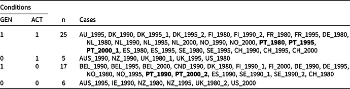
The Portugal cases are highlighted in bold to aid the example discussed below.
Figure 2, using again Portugal as an example, visualizes how the five cases-in-a-country map onto different ideal types over time. This also shows how a certain ideal type’s empirical presence varies over time, relative to that of the other ideal types. The figure can be easily constructed with Excel, by taking the fuzzy-set membership scores for the five cases in each of the four ideal types and then plotting them; it displays the fuzzy-set membership scores in different ways.
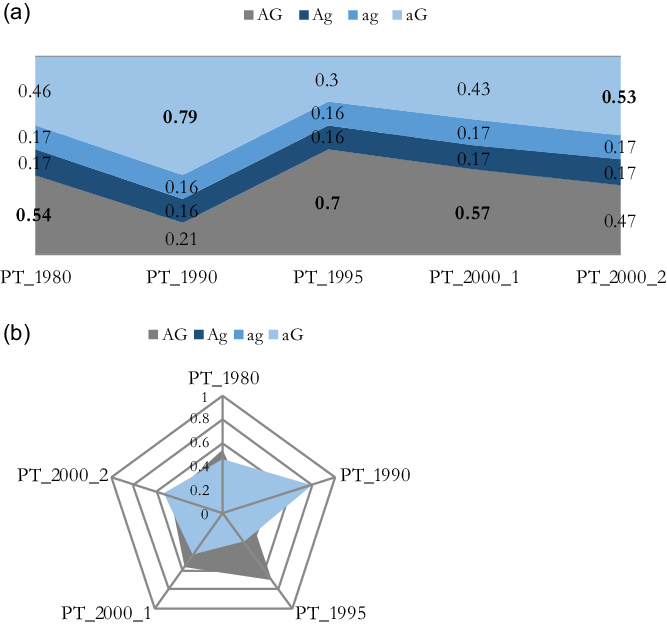
Figure 2. Example of fuzzy-set ideal type analysis for Portugal.
Figure 2 shows how Portugal’s governments moved across the property space over time. In the 1980s, for instance, this case has membership >0.5 to the ideal type AG. In the 1990s, under the third government led by Cavaco e Silva (see Table S.A1), the country had changed to a much less activating welfare state regime; it now had a membership of 0.79 in the ideal type aG. Recall that Portugal’s shift from a generous activating welfare state (AG) to a generous passive welfare state (aG) marks a qualitative shift.Footnote 11 This is perhaps best visible in Figure 2b. In the 1995s, Portugal had changed its welfare state regime back to that of AG, another ideal type (qualitative) shift. From the 1995s to the 2000s (i.e. 2001_1), the country’s welfare state regime became less activating, but not yet to the point that the country could be qualified as a passive welfare state: Portugal was still a member of the ideal type AG. Portugal’s movement from the 1995s to the beginning of the 2000s is, therefore, a quantitative change. This distinction between qualitative and quantitative change corresponds to the notion of difference in-kind and difference in-degree that can be found in the QCA literature on the calibration of sets. The figures can also be read with a focus on the configurations (i.e. ideal types). Then, Figure 2 for instance shows the development of ideal type AG from the 1980s to the 2000s and the relative dominance of this configuration in Portugal for two decades, except for the 1990s under the third government led by Cavaco e Silva.
This example shows how fuzzy-set ideal type analysis can be used to track configurations over time. Some studies also combine this strategy with the strategy of ‘Multiple QCAs, Different Time Periods’ (Strategy B). These studies first conduct a fuzzy-set ideal type analysis, followed by a QCA for each time period with the fuzzy-set membership scores of the different ideal types as the outcomes. Finally, they analyze to what extent the necessary and/or sufficient (combinations of) conditions leading to membership of these ideal types had changed over time (see e.g. Vis et al., Reference Vis, Woldendorp and Keman2013).
Comparison and applicability of the strategies
The three strategies all require data on multiple time points or periods for the same socio-spatial units. In our illustration, the socio-spatial units are countries’ governments and the time periods are the 1980s, 1990s, 1995s, and 2000s. Obviously, the cases need not be countries and can also be meso- or micro-level cases (e.g. organizations, individuals), as long as multiple data points in time for the cases are available. For Strategies A and B, when data are available for only one time period of a socio-spatial unit – that is Austria, Canada, and Ireland in the Vis (Reference Vis2011) dataset – the cases can still be included in the analysis. After all, the interest here is in the solution terms and how they are represented over time (Strategy A) or in the solution formulas and how they differ over time (Strategy B).
In Strategy C, however, it is required that data are available for at least two time points or periods for each socio-spatial unit. The reason is that the interest is in analyzing the trajectory of a case through the property space over time. It is highly preferable to have more than two time points available; with only two time points, the analysis will involve little more than the comparison of two snapshots. All three strategies’ datasets can be analyzed using existing software, in particular the QCA package in R (Duşa, Reference Duşa2019: 209–213).
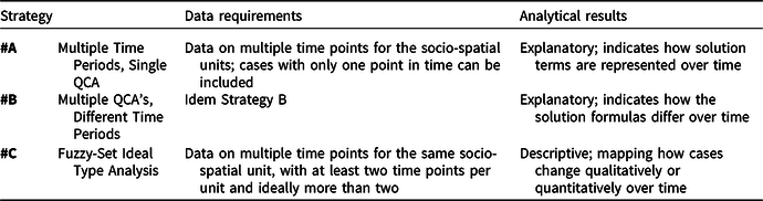
The strategies produce different types of analytical results, meaning that they are suitable for different types of research questions. The results for Strategies A and B express how the solution terms are represented over time or how the solution formulas differ over time. Strategy A allows for mapping the development of cases in terms of how they are represented by different configurations over time or, conversely, of how different configurations are represented by different cases over time. In Strategy B, the results of the multiple truth table minimizations are strung together, creating a time series of minimized configurations. These first two strategies may be particularly useful for more deductive or theory-evaluating research questions (see Thomann and Maggetti, Reference Thomann and Maggetti2020). As such, they also fit well with the ‘realist’, ‘substantive interpretability’ approach to QCA that focusses on finding explanatory configurations for an outcome of interest. What the strategies add compared to a regular, static QCA is that they allow testing whether the configurations are sensitive to era or zeitgeist. Over time, configurational theories, theoretical conjunctures, or configurational hypotheses may require adjustment; and tracking configurations over time with QCA may identify the need for such theoretical adjustments. Fuzzy-set ideal type analysis (Strategy C) distinguishes itself from the other two in that the results are not in the form of solution formulas but instead are a mapping of how a case moves through the property space over time (see Figure 2). This means that it produces rather descriptive results, which are more geared to exploratory and case-focused research questions including, obviously, the creation of typologies (Berg-Schlosser et al., Reference Berg-Schlosser, De Meur, Rihoux, Ragin, Rihoux and Ragin2009). The other two strategies are more explanatory, focused on causal patterns. It also means that the strategies have different configurational foci; Strategy C focusses on the configurational nature of cases, whereas the first two strategies focus on the configurational nature of solution terms or formulas. Table 5 summarizes the similarities and differences in terms of data requirements and analytical results.
Table 5 Differences across strategies: data requirements and analytical results
Finally, the three strategies differ in terms of the research steps involved (cf. Gerrits and Verweij, Reference Gerrits and Verweij2018). In each strategy, the cases are segmented into different time points or periods. The main difference between Strategies A and B, and Strategy C is that the latter does not necessarily involve a truth table analysis. The focus is as said on the construction of an ‘adjusted truth table’ (see Table 4) and a graphical representation thereof (Figure 2). With the first two strategies, instead, the researcher does minimize the truth table(s).
Conclusion
This article has discussed and empirically illustrated three QCA-related strategies that enable political scientists and other researchers to track configurations over time. An issue on the agenda is visualization. As we mentioned, visualization of QCA results can help to better understand them. There are recent, welcome developments in broadening the variety of ways in which QCA results can be visualized (Rubinson, Reference Rubinson2019). However, the visualization of time-sensitive QCA results in general, and the visualization of tracking configurations over time, in particular, has not yet received attention. Here, we have relied mostly on tabular layouts that we crafted manually. To our knowledge, the current QCA software is not yet equipped to accommodate the presentation of the results in the form of the tables as introduced in this article. This is one point that requires attention. Another point on the agenda is the visualization of results in more graphical formats. Whereas it is relatively easy to visualize how cases move through a two-dimensional (e.g. Figure 2) or three-dimensional property space over time, visualizing how solution terms – let alone solution formulas that comprise multiple solution terms – change over time is difficult. Figure 1 is the first attempt, but more work is needed. Especially when research results are complex, which they are increasingly so in Strategies A and B – compared to the regular, static QCAs – visualization is even more important to understand and communicate the results. For the Strategies A and B to get a foothold in QCA research – and for that matter also the other time-sensitive QCA strategies that exist, which are, as said, cited a lot but implemented not – it will help if communicable visualization formats are developed.
Each of the three strategies has its pros and cons. The strategies ‘Multiple Time Periods, Single QCA’ (Strategy A) and ‘Multiple QCAs, Different Time Periods’ (Strategy B) have the advantage that they follow the regular QCA research process and are relatively easy to perform. However, especially Strategy B can only be applied well if the number of conditions per time period is high enough. When the number of cases is rather low – which may regularly be the case in applied QCA – this aggravates the problem of limited diversity. This latter problem is absent in fuzzy-set ideal type analysis (Strategy C); however, it is restricted to the descriptive analysis of cases’ developments only and does hence not allow for a proper explanation. Ultimately, the choice for one, or several, of the strategies depends on the researcher’s research question and the state of the theories at hand.
The strategies discussed here have much potential for researchers who want to track configurations over time. Thus far, there have only been some QCA applications that have done so. We illustrated the strategies with a dataset with 53 cases and 5 conditions. To further the development of the strategies, we invite more empirical applications, involving both less and more cases and conditions, to further tease out their advantages and disadvantages. Still, also without these – welcome – further advancements, the strategies for tracking configurations over time can enrich political scientists’ methodological toolkits. As we have demonstrated, these strategies enable answering a whole series of novel research questions in which time takes a center stage.
Supplementary material
To view supplementary material for this article, please visit https://doi.org/10.1017/S1755773920000375.
Acknowledgments
An earlier version of this paper was presented at the International QCA Expert Workshop in Zurich (2018). We thank the workshop participants, the editors, and the anonymous reviewers for their constructive feedback on the earlier versions of the paper.


 Open access