


1. Introduction
In the standard model, radio pulsars are highly magnetised rapidly rotating neutron stars that emit a coherent light-house beam of often highly polarised radio emission directed by their magnetospheres (Lorimer & Kramer Reference Lorimer and Kramer2004). The weak braking torques caused by their rapidly rotating magnetic fields and their high moments of inertia make them extremely stable flywheels, and it is often possible to predict the pulsar spin period and indeed pulse phase years in advance of observation (Taylor Reference Taylor1992b). Most radio pulsars regularly emit irregular single-pulse shapes that usually sum to an average profile within 1 000 rotations that is often remarkably constant (Liu et al. Reference Liu, Keane, Lee, Kramer, Cordes and Purver2012). Timing of these mean profiles against a template produces an arrival time which can be used to derive a model of the pulsar’s spin-down, astrometric and binary parameters, and propagation through the ionised interstellar medium. The frequency dependence of the pulse arrival time is well described by the cold plasma dispersion relation, and allows observers to compute the column density of free electrons along the line of sight to the observer. The integral of this column density is referred to as the pulsar’s dispersion measure (DM). The most accurate pulse arrival times require observers to remove the broadening of the pulse profile across the finite channel bandwidths using a process known as coherent dedispersion (Hankins & Rickett Reference Hankins and Rickett1975) and accurately monitor changes in the DM (Keith et al. Reference Keith2013).
According to version 1.62 (February 2020) of the Australian Telescope National Facility pulsar catalogueFootnote a (Manchester et al. Reference Manchester, Hobbs, Teoh and Hobbs2005), there are currently 2 800 pulsars known,  $\sim 97\%$
of which are visible at radio wavelengths. Radio pulsars range in pulse period (P) from 1.4 ms to 23.5 s, and have inferred dipolar magnetic field strengths from
$\sim 97\%$
of which are visible at radio wavelengths. Radio pulsars range in pulse period (P) from 1.4 ms to 23.5 s, and have inferred dipolar magnetic field strengths from  $5\times10^7$
to
$5\times10^7$
to  $\sim10^{15}\,\mbox{G}$
. Over 10% of known pulsars are members of binary systems, and the majority of these are the so-called ‘recycled pulsars’ that have had their magnetic fields weakened and spin periods shortened by mass accretion from a donor (Bhattacharya & van den Heuvel Reference Bhattacharya and van den Heuvel1991). The fastest pulsars (
$\sim10^{15}\,\mbox{G}$
. Over 10% of known pulsars are members of binary systems, and the majority of these are the so-called ‘recycled pulsars’ that have had their magnetic fields weakened and spin periods shortened by mass accretion from a donor (Bhattacharya & van den Heuvel Reference Bhattacharya and van den Heuvel1991). The fastest pulsars ( $P<20\,\mbox{ms}$
) are usually referred to as ‘millisecond pulsars’ (MSPs). There pulsars are often in very dynamically clean systems well approximated by point masses and are ideal for tests of gravitational and stellar evolution theories (Weisberg & Huang Reference Weisberg and Huang2016).
$P<20\,\mbox{ms}$
) are usually referred to as ‘millisecond pulsars’ (MSPs). There pulsars are often in very dynamically clean systems well approximated by point masses and are ideal for tests of gravitational and stellar evolution theories (Weisberg & Huang Reference Weisberg and Huang2016).
State-of-the-art pulsar timing allows us to measure pulse arrival times to better than one part in  $10^4$
of the pulse period (van Straten et al. Reference van Straten, Bailes, Britton, Kulkarni, Anderson, Manchester and Sarkissian2001), leading to sub-microsecond arrival times for the MSPs. In their most recent data release (dr2), the International Pulsar Timing ArrayFootnote b lists an rms timing residual for the bright 5.7 ms MSP PSR
$10^4$
of the pulse period (van Straten et al. Reference van Straten, Bailes, Britton, Kulkarni, Anderson, Manchester and Sarkissian2001), leading to sub-microsecond arrival times for the MSPs. In their most recent data release (dr2), the International Pulsar Timing ArrayFootnote b lists an rms timing residual for the bright 5.7 ms MSP PSR  $\mbox{J}0437{-}4715$
of just 110 ns and 14 others with residuals below
$\mbox{J}0437{-}4715$
of just 110 ns and 14 others with residuals below  $1\,\mu\mbox{s}$
(Perera et al. Reference Perera2019).
$1\,\mu\mbox{s}$
(Perera et al. Reference Perera2019).
Modern radio telescopes can detect radio pulsars with a mean flux density (i.e. averaged over the pulse period) down to just a few  $\mu\mbox{Jy}$
in very deep pointings, and the large-scale surveys of much of the galactic plane are complete to
$\mu\mbox{Jy}$
in very deep pointings, and the large-scale surveys of much of the galactic plane are complete to  $\sim0.1\mbox{ mJy}$
(Ng et al. Reference Ng2015). The population exhibits a standard
$\sim0.1\mbox{ mJy}$
(Ng et al. Reference Ng2015). The population exhibits a standard  $\mbox{log}N\mbox{/log}S$
distribution consistent with a largely planar distribution with a slope of approximately
$\mbox{log}N\mbox{/log}S$
distribution consistent with a largely planar distribution with a slope of approximately  $-1$
. The most compelling pulsar science is usually derived from accurate pulse timing which for most pulsars is signal-to-noise limited as the vast majority of known pulsars have flux densities less than 1 mJy at 1 400 MHz. For this reason, the field has been dominated by the world’s largest radio telescopes that possess low-temperature receivers and digital back ends capable of coherently dedispersing the voltages induced in the receiver by the radio pulsars. These telescopes can produce the high signal-to-noise profiles required to test theories of relativistic gravity, determine neutron star masses, clarify the poorly understood radio emission mechanism, and relate the latter to the magnetic field topology.
$-1$
. The most compelling pulsar science is usually derived from accurate pulse timing which for most pulsars is signal-to-noise limited as the vast majority of known pulsars have flux densities less than 1 mJy at 1 400 MHz. For this reason, the field has been dominated by the world’s largest radio telescopes that possess low-temperature receivers and digital back ends capable of coherently dedispersing the voltages induced in the receiver by the radio pulsars. These telescopes can produce the high signal-to-noise profiles required to test theories of relativistic gravity, determine neutron star masses, clarify the poorly understood radio emission mechanism, and relate the latter to the magnetic field topology.
The galactic centre is at declination  $\delta=-29^\circ$
and this makes the Southern hemisphere a particularly inviting location for pulsar studies. For many years, the Parkes 64-m telescope has had almost exclusive access to radio pulsars south of declination
$\delta=-29^\circ$
and this makes the Southern hemisphere a particularly inviting location for pulsar studies. For many years, the Parkes 64-m telescope has had almost exclusive access to radio pulsars south of declination  $\delta=-35^\circ$
, and consequently discovered the bulk of the pulsar population. When choosing a site and host country for the forthcoming Square Kilometre Array (SKA; Dewdney et al. Reference Dewdney, Hall, Schilizzi and Lazio2009) SKA1-mid telescope, the strong pulsar science case made Southern hemisphere locations particularly desirable. MeerKAT (Jonas Reference Jonas2009) is the South African SKA precursor telescope located at the future site of SKA1-mid and the full array has four times the gain (i.e.
$\delta=-35^\circ$
, and consequently discovered the bulk of the pulsar population. When choosing a site and host country for the forthcoming Square Kilometre Array (SKA; Dewdney et al. Reference Dewdney, Hall, Schilizzi and Lazio2009) SKA1-mid telescope, the strong pulsar science case made Southern hemisphere locations particularly desirable. MeerKAT (Jonas Reference Jonas2009) is the South African SKA precursor telescope located at the future site of SKA1-mid and the full array has four times the gain (i.e.  $2.8\,\mbox{K Jy}^{-1}$
) of the Parkes telescope (
$2.8\,\mbox{K Jy}^{-1}$
) of the Parkes telescope ( $0.7\,\mbox{K Jy}^{-1}$
). The first receivers (L-band) to come online possess an excellent system temperature (
$0.7\,\mbox{K Jy}^{-1}$
). The first receivers (L-band) to come online possess an excellent system temperature ( $\sim18\,\mbox{K}$
) along with 856 MHz of recorded bandwidth. The pulsar processor often just records the inner 776 MHz of this for science purposes. The telescope is located at latitude
$\sim18\,\mbox{K}$
) along with 856 MHz of recorded bandwidth. The pulsar processor often just records the inner 776 MHz of this for science purposes. The telescope is located at latitude  $-30^{\circ}43'$
and is ideal for studies of the large population of southern pulsars and those in the Large and Small Magellanic Clouds. Much of pulsar science is signal-to-noise limited until a pulsar hits its ‘jitter limit’ [the lowest timing residual obtainable due to pulse-to-pulse variability in the individual pulses—see Shannon et al. (Reference Shannon2014a)]. When far from the jitter limit, the timing error is inversely proportional to the signal-to-noise ratio. For most pulsars in the Parkes Pulsar Timing Array (PPTA; Manchester et al. Reference Manchester2013), the limit is rarely reached when observed with the Parkes 64-m telescope unless the pulsar is experiencing a scintillation maximum (Shannon et al. Reference Shannon2014b). A notable exception is the bright MSP PSR
$-30^{\circ}43'$
and is ideal for studies of the large population of southern pulsars and those in the Large and Small Magellanic Clouds. Much of pulsar science is signal-to-noise limited until a pulsar hits its ‘jitter limit’ [the lowest timing residual obtainable due to pulse-to-pulse variability in the individual pulses—see Shannon et al. (Reference Shannon2014a)]. When far from the jitter limit, the timing error is inversely proportional to the signal-to-noise ratio. For most pulsars in the Parkes Pulsar Timing Array (PPTA; Manchester et al. Reference Manchester2013), the limit is rarely reached when observed with the Parkes 64-m telescope unless the pulsar is experiencing a scintillation maximum (Shannon et al. Reference Shannon2014b). A notable exception is the bright MSP PSR  $\mbox{J}0437{-}4715$
, that is always jitter-limited when observed at the Parkes telescope (Osłowski et al. 2011) due to its large 1 400 MHz mean flux density of 150 mJy (Dai et al. Reference Dai2015). As telescopes become more sensitive, the number of pulsars in the same integration time being jitter-limited increases.
$\mbox{J}0437{-}4715$
, that is always jitter-limited when observed at the Parkes telescope (Osłowski et al. 2011) due to its large 1 400 MHz mean flux density of 150 mJy (Dai et al. Reference Dai2015). As telescopes become more sensitive, the number of pulsars in the same integration time being jitter-limited increases.
The South African Radio Astronomy Observatory (SARAO) owns and operates MeerKAT and, before it was commissioned, called for Large Survey Projects (LSPs) that could exploit the telescope’s scientific potential. The MeerTimeFootnote c (Bailes et al. Reference Bailes2018) collaboration was successful at obtaining LSP status and commenced its first survey observations in February of 2019. This paper reports on MeerTime’s validation of MeerKAT as a pulsar telescope and presents some early science results from its four major themes: Relativistic and Binary Pulsars, the Thousand Pulsar Array (Johnston Reference Johnston2020), Globular Clusters, and the MeerKAT Pulsar Timing Array.
A glimpse of MeerKAT’s potential as a pulsar telescope was presented in Camilo et al. (Reference Camilo2018) when it was part of a campaign that observed the revival of the magnetar PSR  $\mbox{J}1622{-}4950$
. Since then there have been a number of developments of the system that enable a wider range of pulsar observing modes that will be discussed forthwith.
$\mbox{J}1622{-}4950$
. Since then there have been a number of developments of the system that enable a wider range of pulsar observing modes that will be discussed forthwith.
The structure of this paper is as follows: In Section 2, we provide an overview of MeerKAT as a pulsar telescope including examples of the Ultra-High Frequency (UHF) and L-band radio bands, the Precise Time Manager (PTM), choice of polyphase filter banks (PFBs), and the SKA1 prototype pulsar processor PTUSE developed by Swinburne University of Technology. In Section 3, we describe our validation of the system and pulsar hardware before presenting new science from observations of selected pulsars and globular clusters in Section 4. Finally, we briefly discuss some of the prospects for the future of this facility including new modes, receivers, and extensions and ultimate extension to become SKA1-mid in Section 5.
2. The MeerKAT telescope as a pulsar facility
A high-level block diagram of the system is provided in Figure 1 that describes the system all the way from the antennas to the final data product archive. The back-end system design largely followed the CASPER philosophy of transferring as much of the transport between the digital subsystems to commodity-off-the-shelf (COTS) components and industry standard protocols (e.g. ethernet) that involve commercial switches and are interfaced to the pulsar processor which is itself a modern server comprised entirely of COTS components.
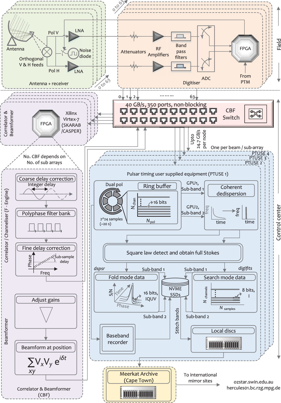
Figure 1. A block diagram of the signal chain for MeerTIME observations. Signals from all antennas are digitised in the field and sent to the correlator–beamformer (CBF) engine in the building via the CBF switch. For pulsar observations, CBF performs channelisation (1K or 4K mode) and beamforms at the requested sky position. The beamformed voltages are sent to the PTUSE machines via the CBF switch at a data rate of up to  $24.7 \mbox{Gb s}^{-1}$
. Each PTUSE node can process one beam/sub-array. In each PTUSE node, the incoming voltages are temporarily stored in a ring buffer from which they are sent to the two GPUs, each processing one half of the band. The GPUs perform coherent dedispersion and square law detection to obtain 16-bit, full Stokes data, which, depending on the observation, is either folded into pulsar archives or scrunched into 8-bit, total intensity filter bank data. The GPUs write the end products to the NVME discs via the CPUs, from which the two bands are stitched together and transferred to the local discs. The baseband recorder, when triggered, can dump baseband data to the NVME discs for a period of about 40 min. The data from the local discs are eventually transferred to the MeerKAT archive in Cape Town, from which they are transferred to international mirror sites.
$24.7 \mbox{Gb s}^{-1}$
. Each PTUSE node can process one beam/sub-array. In each PTUSE node, the incoming voltages are temporarily stored in a ring buffer from which they are sent to the two GPUs, each processing one half of the band. The GPUs perform coherent dedispersion and square law detection to obtain 16-bit, full Stokes data, which, depending on the observation, is either folded into pulsar archives or scrunched into 8-bit, total intensity filter bank data. The GPUs write the end products to the NVME discs via the CPUs, from which the two bands are stitched together and transferred to the local discs. The baseband recorder, when triggered, can dump baseband data to the NVME discs for a period of about 40 min. The data from the local discs are eventually transferred to the MeerKAT archive in Cape Town, from which they are transferred to international mirror sites.
2.1. The MeerKAT radio frequency spectrum
MeerKAT is located in the Karoo, some 450 km north-east of Cape Town in the Northern Cape Province. Its low population density makes it an attractive site to pursue radio astronomy. The low-frequency HERA experiment (DeBoer et al. Reference DeBoer2017) and the future 197-dish SKA1-mid telescope (Dewdney et al. Reference Dewdney, Hall, Schilizzi and Lazio2009)—of which MeerKAT will be a part—will be located at the site which is protected by legislation against radio transmissions in many bands of relevance to radio astronomers.
The technology behind low-noise amplifiers and radio receivers has greatly improved since the dawn of radio astronomy in the 1950s. Whilst even just a couple of decades ago it was necessary to sacrifice fractional bandwidth to minimise system temperature new engineering practices and technologies now permit the development of low-noise ( $\sim20\,\mbox{K}$
) receivers over a full octave or more of bandwidth, e.g. Hobbs et al. (Reference Hobbs2019).
$\sim20\,\mbox{K}$
) receivers over a full octave or more of bandwidth, e.g. Hobbs et al. (Reference Hobbs2019).
The original MeerKAT radio telescope specification had a target effective collecting area per unit receiver temperature of  $A_{\rm eff}/T = 220\,\mbox{m}^2\mbox{ K}^{-1}$
but remarkably achieved 350–450
$A_{\rm eff}/T = 220\,\mbox{m}^2\mbox{ K}^{-1}$
but remarkably achieved 350–450  $\mbox{m}^2\mbox{ K}^{-1}$
(depending upon radio frequency), well over a factor of 2 increase in observing efficiency over the design specification. These figures equate to a system equivalent flux density (SEFD) of
$\mbox{m}^2\mbox{ K}^{-1}$
(depending upon radio frequency), well over a factor of 2 increase in observing efficiency over the design specification. These figures equate to a system equivalent flux density (SEFD) of  $\textrm{SEFD}=T/G\sim7\,\mbox{Jy}$
, where T is the system temperature in K and G is the total antenna gain
$\textrm{SEFD}=T/G\sim7\,\mbox{Jy}$
, where T is the system temperature in K and G is the total antenna gain  $G= A{\eta}/(2k)$
, A is the collecting area,
$G= A{\eta}/(2k)$
, A is the collecting area,  $\eta$
is the aperture efficiency, and k is Boltzmann’s constant. The total MeerKAT antenna gain is
$\eta$
is the aperture efficiency, and k is Boltzmann’s constant. The total MeerKAT antenna gain is  $2.8\,\mbox{K Jy}^{-1}$
and the system temperature about 18 K in the optimal location of the 1 400 MHz band. The receivers have two orthogonal linear polarisations (H and V for horizontal and vertical, respectively).
$2.8\,\mbox{K Jy}^{-1}$
and the system temperature about 18 K in the optimal location of the 1 400 MHz band. The receivers have two orthogonal linear polarisations (H and V for horizontal and vertical, respectively).
In Figure 2, we present the radio spectrum as observed from the MeerKAT site for the UHF (544–1 088 MHz) and L-band (856–1 712 MHz) receivers taken from observations of the double pulsar PSR  $\mbox{J}0737{-}3039\mbox{A}$
. Pulsar observations are usually made with 1 024 or 4 096 frequency channels. The UHF band is remarkably clean, with just some small (strong but narrow-bandwidth) residual mobile phone-related transmissions visible around 940 MHz. In most countries that house large-diameter (64 m class and above) telescopes, the UHF band is so badly polluted by digital television and mobile phone transmissions that it is often unusable except in very narrow frequency windows some 10 s of MHz wide. Both of the SKA sites appear to have been chosen well and offer a renewed opportunity to explore the Universe at these frequencies. For pulsars, this is especially relevant, as most possess steep spectra (Jankowski et al. Reference Jankowski, van Straten, Keane, Bailes, Barr, Johnston and Kerr2018; Maron et al. Reference Maron, Kijak, Kramer and Wielebinski2000; Toscano et al. Reference Toscano, Bailes, Manchester and Sandhu1998), with spectral indices of between
$\mbox{J}0737{-}3039\mbox{A}$
. Pulsar observations are usually made with 1 024 or 4 096 frequency channels. The UHF band is remarkably clean, with just some small (strong but narrow-bandwidth) residual mobile phone-related transmissions visible around 940 MHz. In most countries that house large-diameter (64 m class and above) telescopes, the UHF band is so badly polluted by digital television and mobile phone transmissions that it is often unusable except in very narrow frequency windows some 10 s of MHz wide. Both of the SKA sites appear to have been chosen well and offer a renewed opportunity to explore the Universe at these frequencies. For pulsars, this is especially relevant, as most possess steep spectra (Jankowski et al. Reference Jankowski, van Straten, Keane, Bailes, Barr, Johnston and Kerr2018; Maron et al. Reference Maron, Kijak, Kramer and Wielebinski2000; Toscano et al. Reference Toscano, Bailes, Manchester and Sandhu1998), with spectral indices of between  $-1$
and
$-1$
and  $-3$
above 1 GHz.
$-3$
above 1 GHz.

Figure 2. The post-calibration bandpasses of a tied-array beam, for MeerKAT’s UHF and L-band receivers. The flux density scale is arbitrary. It is often difficult to completely flatten the band in regions of persistent interference such as that near 1 530–1 600 MHz.
The 1 400-MHz (L-band) receiver band is not as pristine as the UHF band, but still has much of the spectrum available for science (see a quantified analysis in the following), depending upon the flux density of the target pulsar. The tied-array beam helps dilute interfering signals by dephasing them but the large number of bits in the digitisers and beam former that deliver accurate channelisation of the data have one drawback in the sense that the interference-to-noise ratio can be extremely high. This makes deletion of at least some frequency channels essential before integration across frequency channels.
Like all modern observatories, the 1 400 MHz band suffers from transmissions from Global Navigation Satellite Systems (GNSS) and other satellites that are extremely strong and impossible to avoid. The small apertures (and hence large side lobes) that the 14-m dishes of MeerKAT provide make satellite transmissions in the band almost omnipresent. The L-band spectrum is shown in Figure 2(b).
The first of the S-band ( $1.75$
–
$1.75$
– $3.5\,\mbox{GHz}$
) receivers of the Max-Planck-Institut für Radioastronomie (Kramer et al. Reference Kramer2016) are currently being installed and tested. When fully installed, these will provide the possibility of performing high-precision timing at even higher frequencies.
$3.5\,\mbox{GHz}$
) receivers of the Max-Planck-Institut für Radioastronomie (Kramer et al. Reference Kramer2016) are currently being installed and tested. When fully installed, these will provide the possibility of performing high-precision timing at even higher frequencies.
2.2. Precise time systems in MeerKAT
2.2.1. Background on requirements
The SKA phase I (comprising SKA1-low and SKA1-mid) has been strongly motivated by two key science projects, the Epoch of Reionisation and strong-field tests of gravity, respectively (e.g. Kramer et al. Reference Kramer2016). Despite the advent of direct gravitational wave detection (Abbott et al. Reference Abbott2016) and black hole imaging (Event Horizon Telescope Collaboration et al. Reference Event Horizon Telescope2019), a number of precision strong-field tests can only be achieved at radio wavelengths using pulsars. This includes the detection of a gravitational wave background from supermassive black holes using pulsar timing arrays (e.g. Arzoumanian et al. Reference Arzoumanian2018b; Lentati et al. Reference Lentati2015; Shannon et al. Reference Shannon2015), which will require timing an ensemble of MSPs to precisions well below 100 ns and possibly down to 10 ns. In order to achieve such precisions, two of the SKA1 specifications are especially relevant, one related to the calibration of the polarimetry that otherwise leads to systematic errors in timing, see, e.g., Foster et al. (Reference Foster, Karastergiou, Paulin, Carozzi, Johnston and van Straten2015), and the other the knowledge of absolute time with respect to Coordinated Universal Time (UTC) over a full decade. The SKA1-mid specification on calibratable polarisation purity is  $-40\,\mbox{dB}$
, and on time 5 ns over 10 yr.
$-40\,\mbox{dB}$
, and on time 5 ns over 10 yr.
The precise time systems in MeerKAT are specified to provide time products accurate to better than 5 ns, relative to UTC. The telescope was designed for absolute, not just relative timing which is the norm. This is achieved via a first-principles approach, by managing the time delays associated with every element of the geometric and signal paths.
2.2.2. Realisation of system timing for the MeerKAT telescope
MeerKAT has defined a reference point on the Earth to which all time is referred. It is a location a few hundred metres approximately north of the centre of the array with the ITRF coordinates  $X=5\,109\,360.0$
,
$X=5\,109\,360.0$
,  $Y=2\,006\,852.5$
,
$Y=2\,006\,852.5$
,  $Z= -3\,238\,948.0\,\mbox{m}$
.
$Z= -3\,238\,948.0\,\mbox{m}$
.  $\pm0.5\mbox{ m}$
. The position of the reference point was chosen as the circumcentre of the array, roughly a metre above the ground. There is no antenna at this point; all pulsar timing is ultimately referred to when an incident radio wave would have struck this point. This location for MeerKAT is installed in the observatory coordinate file for the pulsar timing software tempo2 (Hobbs, Edwards, & Manchester Reference Hobbs, Edwards and Manchester2006), and used for all work in this paper.
$\pm0.5\mbox{ m}$
. The position of the reference point was chosen as the circumcentre of the array, roughly a metre above the ground. There is no antenna at this point; all pulsar timing is ultimately referred to when an incident radio wave would have struck this point. This location for MeerKAT is installed in the observatory coordinate file for the pulsar timing software tempo2 (Hobbs, Edwards, & Manchester Reference Hobbs, Edwards and Manchester2006), and used for all work in this paper.
The coordinates of the source, antenna, and UT1 define the geometric delay, and every attempt is made to derive the further delays incurred by the signal as it reflects off the telescope surfaces, passes through the feed/receiver/cable/filter, and is ultimately sampled by the analogue-to-digital converters (ADCs). Round-trip measurements account for cable and fibre delays and are accurate to typically 1 ns. Estimates of the error in each stage of the path are also recorded for later dissemination to the pulsar processor to be recorded with the data.
At each antenna, a digitiser is mounted close to the focus (see the lower panel in Figure 3). The digitiser ADC is driven by the digitiser sample clock, derived from the Maser frequency standards and disseminated directly to the digitisers by optical fibre. The input voltages are sampled at the Nyquist rate after passing through an analogue filter for the selected band. The L-band receiver digitises the data at exactly 1 712 MHz (real samples) and passes the second Nyquist zone (i.e. top half of the band 856–1 712 MHz) to the CBF via optical fibre Ethernet. The digitiser maintains a 48-bit ADC sample counter, used to tag every packet. The counter is reset every day or two by telescope operators, before it overflows. The 10-bit digitiser offers excellent resistance to radio frequency interference (RFI) and makes it possible to confine RFI to only the relevant frequency channels unless it causes saturation of the ADC.

Figure 3. MeerKAT time systems showing time transfer from GNSS, the local clock ensemble, and transfer of time to the digitisers. Here Rb stands for the element Rubidium, and WR is the White Rabbit sub-ns accuracy Ethernet-based time transfer system. PPS is the 1 pulse per second used in precision timing experiments, and FPGAs are Field Programmable Gate Arrays. See text for further details.
Optical timing pulses are generated by the Time and Frequency Reference (TFR) system in the processor building and disseminated to all antennas via dedicated optical fibres. The digitiser records the time of arrival of the optical pulse from the masers; it is also used to reset the digitiser sample clock when necessary. The timing fibres are buried 1 m deep to minimise diurnal temperature variations, but change length over the year as the site temperature varies. A round-trip measurement system continuously measures their length by timing the round trip of the timing pulse as reflected back from the digitiser (Adams et al. Reference Adams2018; Siebrits et al. Reference Siebrits and du Plessis2017). This falls within a general class of time-of-flight measurement which is traceable to the SI unit of time (Terra & Hussein Reference Terra and Hussein2015).
In the correlator, prior to channelisation, the signals from all antennas are buffered and aligned using the ADC sample counter. Integer samples of delay are applied to compensate for physical delays. A multi-tap Hann-window PFB is used to filter the data along with a phase gradient to eliminate the remaining (sub-sample) geometrical delay. Pulsar timing observations at L-band usually use the 1 024 channel mode, giving a time resolution of  $1/B$
of
$1/B$
of  $1.196\,\mu\mbox{s}$
. The narrowest mean MSP profile features are 10s of
$1.196\,\mu\mbox{s}$
. The narrowest mean MSP profile features are 10s of  $\mu\mbox{s}$
in width although ‘giant’ pulses have been observed with time resolution from the Crab pulsar with timescales of down to 1 ns (Hankins et al. Reference Hankins, Kern, Weatherall and Eilek2003).
$\mu\mbox{s}$
in width although ‘giant’ pulses have been observed with time resolution from the Crab pulsar with timescales of down to 1 ns (Hankins et al. Reference Hankins, Kern, Weatherall and Eilek2003).
The PTM is a program that collects and aggregates all known delays in the system: geometric, physical delays in the antenna, analogue and digital delays in the receiver and digitiser, the correlator delay, and the digitiser clock offset. PTM computes the time that the wavefront corresponding to a certain ADC sample crossed the array phase centre, and the uncertainty in this time. This time is passed to PTUSE for recording in the header of the pulsar observation. In September 2019, the uncertainty in this value was 3–4 ns.
2.2.3. Tracking of telescope time: Karoo Telescope Time
The station clock is referred to as KTT (Karoo Telescope Time). This timescale is generated by the TFR subsystem using an ensemble of two active hydrogen masers, two Rubidium clocks, and a quartz crystal. It is a physical timescale, defined at a connector in the system. The masers drift by typically just a few nanoseconds per day; KTT is kept  $\sim1\,\mu\mbox{s}$
from UTC by adjusting their synthesised frequency every few months to keep them in defined offset bands.
$\sim1\,\mu\mbox{s}$
from UTC by adjusting their synthesised frequency every few months to keep them in defined offset bands.
The TFR system provides a 10 MHz frequency reference, from the Maser currently in use. Fractional frequency offset is kept to smaller than  $2\times10^{-13}$
with respect to UTC; no significant drift in time occurs during any observing campaign. Frequency synthesisers in the building, one per band, are locked to the reference frequency and generate the 1 712 and 1 088 MHz sample clocks for distribution to the digitisers.
$2\times10^{-13}$
with respect to UTC; no significant drift in time occurs during any observing campaign. Frequency synthesisers in the building, one per band, are locked to the reference frequency and generate the 1 712 and 1 088 MHz sample clocks for distribution to the digitisers.
The TFR also provides accurate time to other components of the telescope via Precision Time Protocol (PTP): this is used amongst other things in the pointing of the telescope and control of the precision timing systems (Adams et al. Reference Adams2018).
Pulsar timing requires the difference between UTC and KTT to be measured. At MeerKAT, this is done with a set of calculations to calculate ensemble time using interclock differences between five clocks, and measurements of four clocks with respect to GPS via two dual-band GNSS receivers and two single-band GPS-only receivers (Burger et al. Reference Burger, Siebrits, van Tonder, Adams, Welz, Ramudzuli, Kapp and du Plessis2019). The multiple measurements then lead to clock solutions for each of the clocks in the ensemble via linear combinations of the different measurements. The usage of multiple clocks enables error/instability detection in any one of the clocks and a lower variance estimate in any one of the clocks as with standard ensembling used in timescale generation (Levine Reference Levine2012).
Reference is made to the UTC via common-view comparison with the National Metrology Institute of South Africa (NMISA) in Pretoria, and by direct comparison with UTC(USNO) via GPS time dissemination. The uncertainty of the absolute time difference between KTT and UTC is specified to be less than 5 ns. At present, the systematic (non-varying) offset is only stated to 50 ns due to verification of absolute offset calibration being undertaken. The offset calibration was performed using absolutely calibrated GPS receivers before main observations were being undertaken, and will in future be done using an electromagnetic compatibility-quiet calibrator (Gamatham et al. Reference Gamatham2018) in order not to disrupt the observations. The repeatability between observations is thought to be about 5 ns, implying that the systematics and the stability will finally converge to the latter number; final absolute calibration via a GPS simulator traceability chain will lower the absolute offset to <1 ns. As we shall see later on, there is evidence from our pulsar timing results that we are approaching these levels of clock correction/stability. Furthermore, the clock tracker is currently being improved from a semi-real time predictive method, to a fully post facto non-causal filtering type, using Savitzky–Golay filtering (Savitzky & Golay Reference Savitzky and Golay1964) on which provisional internal self-consistency checks suggest a numerical error of <1 ns. Post facto (Levine Reference Levine2012), non-causal calculation is always better in improving timing compared to real-time ‘UTC-like’ timescale estimation, due to an increased data set, administrative oversight, ability to correct for non-idealities, and the inherent outperformance of smoothers as compared to causal filters (Einecke Reference Einecke2012; Jensen et al. Reference Jensen and Benesty2012).
2.3. The polyphase filter banks
The MeerKAT channeliser (the F-engine) uses a PFB to channelise the digitised bandwidth into 1 024 or 4 096 critically sampled frequency channels with configurations described in Table 1. A PFB filter design with a 16-tap Hann window was deployed aiming to achieve high sensitivity for continuum mapping with minimal bandwidth losses. This design uses only 6 dB of attenuation at the channel edges which however gives rise to significant aliasing from adjacent channels in pulsar observations. To address this, an alternate 16-tap Hann window design that provides superior spectral purity performance at a modest price in sensitivity (due to reduced effective bandwidth) was implemented. This was achieved by reducing the 6 dB cut-off frequency to 0.91 times the channel width, sacrificing  $\sim5\%$
of the sensitivity to reduce the leakage by 10 dB. Delay compensation is done in the F-engine. The requested delay polynomial is re-computed at every Fast Fourier Transform. Coarse delay is done with a whole-sample delay buffer before the PFB. Fine delay is applied by phase rotation after the PFB. The channelised voltages in each packet from the F engine are timestamped with the same 48-bit counter as the original digitiser voltages, delayed by the delay tracking system, and the impulse response of the channeliser. The F-engine operates internally with 22-bit complex numbers; these are requantised to 8 bits real + 8 bits imaginary for transmission over the network. The requantisation gain is chosen to provide adequate resolution on the quietest channels, which results in some of the strongest RFI channels being clipped. The requantisation gain register is also used to flatten the bandpass, equalise the gain of H and V polarisations, and correct for per-channel phase variations found during phase-up.
$\sim5\%$
of the sensitivity to reduce the leakage by 10 dB. Delay compensation is done in the F-engine. The requested delay polynomial is re-computed at every Fast Fourier Transform. Coarse delay is done with a whole-sample delay buffer before the PFB. Fine delay is applied by phase rotation after the PFB. The channelised voltages in each packet from the F engine are timestamped with the same 48-bit counter as the original digitiser voltages, delayed by the delay tracking system, and the impulse response of the channeliser. The F-engine operates internally with 22-bit complex numbers; these are requantised to 8 bits real + 8 bits imaginary for transmission over the network. The requantisation gain is chosen to provide adequate resolution on the quietest channels, which results in some of the strongest RFI channels being clipped. The requantisation gain register is also used to flatten the bandpass, equalise the gain of H and V polarisations, and correct for per-channel phase variations found during phase-up.
Table 1. MeerKAT F-Engine Configurations, with each producing dual polarisations quantised to 8 bits per sample. Frequencies and bandwidths are quoted in MHz and the sampling interval in microseconds.

The F-engine PFB implementation lowers the precise centre frequency of all channels by half a fine channel width (i.e. by  $BW / N_{\rm chan} / 2$
), where BW is the total bandwidth. For example, the precise centre frequency of the first channel for L-band with 1 024 channels is 856 MHz.
$BW / N_{\rm chan} / 2$
), where BW is the total bandwidth. For example, the precise centre frequency of the first channel for L-band with 1 024 channels is 856 MHz. $^{\dagger}$
The F-engine PFB implementation lowers the precise centre frequency of all channels by half a fine channel width (i.e. by
$^{\dagger}$
The F-engine PFB implementation lowers the precise centre frequency of all channels by half a fine channel width (i.e. by  $BW / N_{\rm chan} / 2$
), where BW is the total bandwidth. For example, the precise centre frequency of the first channel for L-band with 1 024 channels is 856 MHz.
$BW / N_{\rm chan} / 2$
), where BW is the total bandwidth. For example, the precise centre frequency of the first channel for L-band with 1 024 channels is 856 MHz.
A comparison of the shape of the transfer function for the two modes is shown in Figure 4. The level magnitude response at channel boundaries (–0.5 and +0.5) determine the level of spectral leakage artefacts in pulsar timing observations. This effect is discussed in Section 3.3, which shows the 0.91 filter design greatly reduces the artefacts and hence why this design has been deployed for most MeerTime observations (exceptions are those made with the 4 096 channel mode).
2.4. The beamformer
The MeerKAT beamformer (the B-engine) creates a dual polarisation tied-array beam by adding together the channelised complex voltages for all antennas, as produced by their individual F-engines. Thus the beam is also Nyquist-sampled like the antenna voltages. The B-engine is distributed among (typically) 64 SKARABs custom boards developed by SARAO for digital signal processing designed to be used with the CASPER tools Hickish et al. Reference Hickish2016), each processing a subset of frequencies for all antennas. Samples are aligned by a timestamp before addition. A per-antenna real gain is provided for beam shaping; this is generally left at unity, but can be set to zero to eliminate an antenna from the beam, perhaps if it is not working properly. The B-engine output is also an 8-bit complex number and uses a requantisation gain to scale down the sum of the antenna voltages; this is typically scaled by  $1/\sqrt{N_{\rm ants}}$
. The output data is sent back onto the switch as speadFootnote d streams, one for each polarisation, using UDP multi-cast for consumption by downstream users. The packet sizes and rates are listed in Table 2. The B-engine can produce up to four tied-array beams from up to four simultaneous sub-arrays for downstream processing by the PTUSE pulsar processing servers. The computational burden on each server is identical regardless of the number of antennas in the sub-array.
$1/\sqrt{N_{\rm ants}}$
. The output data is sent back onto the switch as speadFootnote d streams, one for each polarisation, using UDP multi-cast for consumption by downstream users. The packet sizes and rates are listed in Table 2. The B-engine can produce up to four tied-array beams from up to four simultaneous sub-arrays for downstream processing by the PTUSE pulsar processing servers. The computational burden on each server is identical regardless of the number of antennas in the sub-array.
Table 2. MeerKAT B-engine output configurations, based on the F-engine sampling interval and data rates.
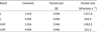

Figure 4. Magnitude response of the two evaluated channeliser filter designs. The original filter design (dashed) led to significant artefacts in pulsars with high ratios of DM to period—see text.
Table 3. PTUSE hardware deployments, detailing the hardware configuration of the commissioning and deployment systems used with MeerTIME.
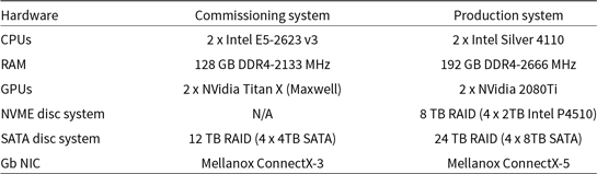
Table 4. PTUSE processing capabilities.

With polarisations H and V, 1 denotes Stokes I (HH + VV), 2 denotes the square law detected power for each polarisation (HH, VV), and 4 denotes the square law detected power in each polarisation and the real and imaginary components of the covariance between the polarisations (HH, VV, Real(H*V), Imag(H*V)). $^{\dagger}$
With polarisations H and V, 1 denotes Stokes I (HH + VV), 2 denotes the square law detected power for each polarisation (HH, VV), and 4 denotes the square law detected power in each polarisation and the real and imaginary components of the covariance between the polarisations (HH, VV, Real(H*V), Imag(H*V)).
$^{\dagger}$
With polarisations H and V, 1 denotes Stokes I (HH + VV), 2 denotes the square law detected power for each polarisation (HH, VV), and 4 denotes the square law detected power in each polarisation and the real and imaginary components of the covariance between the polarisations (HH, VV, Real(H*V), Imag(H*V)).
2.5. PTUSE: An SKA pulsar processing prototype
PTUSE stands for Pulsar Timing User Supplied Equipment in the standard SARAO nomenclature. This sub-system receives channelised voltage time series from the B-engines. Each of the tied-array beams are received on separate high end server class machines and processed to produce reduced data products which are then transferred to the MeerKAT data archive for long-term storage and subsequent processing. The system design was developed by Swinburne University of Technology as the pulsar timing prototype for SKA pre-construction.
Two commissioning servers were deployed in 2015 for development and early science activities and were used until December 2019. Four production servers were then deployed to be used for the MeerTime key science program, allowing for increased processing capabilities and simultaneous processing of four tied-array beams. The configuration of servers for each deployment is described in Table 3.
Each PTUSE server subscribes to two spead streams from the B-engines via a tree of Mellanox 40 Gb switches, one for each polarisation. The spipFootnote e software library receives the two streams, merging them and writing them to a psrdadaFootnote f ring buffer in CPU memory. The ring buffer is configured to hold approximately 20 s of data, providing buffer space to absorb any downstream processing lag. The ring buffer uses shared memory to facilitate asynchronous I/O between the smaller, faster writes of the UDP receive process and the larger, slower reads of the signal processing software. Monitoring software can also periodically sample the data streams to provide signal displays and diagnostics.
Regardless of the number of channels, the data are split into two equal sub-bands which are independently processed in parallel by the pipelines in the dspsr (van Straten & Bailes Reference van Straten2011) software library. The pipelines perform the major signal processing functions on the GPUs which provide sufficient performance to process sub-bands in real time. dspsr performs coherent dedispersion and can produce folded pulsar profiles (fold mode) or filter banks (filter bank mode), significantly reducing the output data rate. The fold mode and filter bank mode both support flexible configuration parameters defining the output data resolutions subject to the limits listed in Table 4.
Both fold-mode and filter bank-mode data write the sub-banded results to disc in psrfits (Hotan, van Straten, & Manchester Reference Hotan, van Straten and Manchester2004) format, which are subsequently combined into a single file and transferred to both the MeerKAT Data Archive and the Swinburne OzSTAR supercomputer. The volume of filter bank data can be extreme when observing at the highest filter bank time resolutions, typical of globular cluster observing, recording data at over  $400\,\mbox{MB s}^{-1}$
(
$400\,\mbox{MB s}^{-1}$
( $30\,\mbox{TB day}^{-1}$
). These data products may be reduced on machines on-site prior to transfer to the data archive but also copied to future mirror sites planned in Europe (e.g. Max Planck Institute für RadioAstronomie).
$30\,\mbox{TB day}^{-1}$
). These data products may be reduced on machines on-site prior to transfer to the data archive but also copied to future mirror sites planned in Europe (e.g. Max Planck Institute für RadioAstronomie).
2.6. PTUSE: Challenges and upgrades
During commissioning, it was found that capture of small UDP multi-cast packets at the high rates required is challenging on the Intel E5-2623v3 CPUs in the Commissioning System. The Commissioning System suffered from occasional packet loss, with an average loss rate of 700 bytes per minute (less than about 4 parts per billion) when observing at L-band in 1 024 channel mode. Rather than having ‘holes’ in the data, the samples from the previous cycle of the ring buffer were used to maintain the system noise level. This can occasionally replace what should be system noise by a pulse and vice versa. The issue was traced to insufficient CPU memory bandwidth, and to eliminate potential artefacts, the switch to the Production System has eliminated virtually all packet loss.
PTUSE supports a raw baseband observing mode which records the raw channelised voltage time series produced by the B-engines. The Commissioning Systems could only store  $<30\,\mbox{s}$
of data in this mode which would then require many minutes to slowly write out to the SATA disc system. The Production Systems each feature an Non-volatile memory express RAID disc which can record at 6 GB
$<30\,\mbox{s}$
of data in this mode which would then require many minutes to slowly write out to the SATA disc system. The Production Systems each feature an Non-volatile memory express RAID disc which can record at 6 GB  $\mbox{s}^{-1}$
, which adds the capability to record up to 40 min of raw baseband data to disc on each server. This baseband mode allows recording at the native
$\mbox{s}^{-1}$
, which adds the capability to record up to 40 min of raw baseband data to disc on each server. This baseband mode allows recording at the native  $1.196\, \mu\mbox{s}$
time resolution of the PFB channel bandwidths, enabling the study of giant pulses, pulse microstructure or the timing of many globular cluster pulsars at Nyquist time resolution upon playback.
$1.196\, \mu\mbox{s}$
time resolution of the PFB channel bandwidths, enabling the study of giant pulses, pulse microstructure or the timing of many globular cluster pulsars at Nyquist time resolution upon playback.
The Commissioning Systems will be retained for data distribution and monitoring with the Production Systems used for all future PTUSE observations.
The dspsr software library supports the creation of multiple frequency channels within each coarse channel (using the −F option on the command line) but to date there has been no call for it from observers and the user interface does not yet support it. Writing baseband data to disc and running dspsr on the command line would achieve this functionality if required.
3. System verification
3.1. System equivalent flux density
Most pulsars at high DM (i.e. with  $\mbox{DM} > 200\,\mbox{pc\,cm}^{-3}$
) show only modest (
$\mbox{DM} > 200\,\mbox{pc\,cm}^{-3}$
) show only modest ( $< 1 \mbox{dB}$
) flux density variation at the MeerKAT observing frequencies and can be used to perform a first-order calibration of the system performance. Three such pulsars are PSRs
$< 1 \mbox{dB}$
) flux density variation at the MeerKAT observing frequencies and can be used to perform a first-order calibration of the system performance. Three such pulsars are PSRs  $\mbox{J}1602{-}5100$
(
$\mbox{J}1602{-}5100$
( $\mbox{B}1558{-}50$
),
$\mbox{B}1558{-}50$
),  $\mbox{J}1651{-}4246$
(
$\mbox{J}1651{-}4246$
( $\mbox{B}1648{-}42$
), and
$\mbox{B}1648{-}42$
), and  $\mbox{J}1809{-}1917$
with flux densities of 7.0, 21.4, and 2.8 mJy at 1 369 MHz as measured by the Parkes telescope (Johnston & Kerr Reference Johnston and Kerr2018). Each of these pulsars was observed on four separate occasions with MeerKAT using the L-band receiver and here we investigate the system performance they imply for the telescope. The data were excised of interference and split into two bands each of 194 MHz centred near 1 200 and 1 400 MHz in order to best compare with the Parkes data. We derived an SEFD (including the sky contribution) of 8.1, 8.0, and 10.3 Jy in the central part of the band for the three pulsar locations. It is difficult to accurately estimate the sky contribution with the current MeerKAT system, but the Parkes observations would imply values of 4, 4, and 10 K in the direction of the three pulsars. We therefore conclude that the SEFD is consistent with 7 Jy across 400 MHz of bandwidth.
$\mbox{J}1809{-}1917$
with flux densities of 7.0, 21.4, and 2.8 mJy at 1 369 MHz as measured by the Parkes telescope (Johnston & Kerr Reference Johnston and Kerr2018). Each of these pulsars was observed on four separate occasions with MeerKAT using the L-band receiver and here we investigate the system performance they imply for the telescope. The data were excised of interference and split into two bands each of 194 MHz centred near 1 200 and 1 400 MHz in order to best compare with the Parkes data. We derived an SEFD (including the sky contribution) of 8.1, 8.0, and 10.3 Jy in the central part of the band for the three pulsar locations. It is difficult to accurately estimate the sky contribution with the current MeerKAT system, but the Parkes observations would imply values of 4, 4, and 10 K in the direction of the three pulsars. We therefore conclude that the SEFD is consistent with 7 Jy across 400 MHz of bandwidth.
3.2. Bandwidth utilisation
To quantify the effect of RFI on our pulsar science, we took observations of the narrow duty-cycle MSP PSR  $\mbox{J}1909{-}3744$
from Feb 2019 until Nov 2019 and eliminated interference by looking for deviations in the pulsar’s baseline that exceeded 5 sigma after averaging the pulse profile every 8 s. In total, we analysed 2 825 8-s integrations. These results are shown in Figure 5. In the central 928 channels of the 1 024, we only had to delete 12.8% of the 1 400 MHz band, on average. Although, some of these channels have very persistent RFI and their deleted fraction is close to 100%, particularly those channels associated with Global Positioning Satellites and the mobile phone band near 950 MHz. Other RFI sources are very time-dependent like those associated with aircraft.
$\mbox{J}1909{-}3744$
from Feb 2019 until Nov 2019 and eliminated interference by looking for deviations in the pulsar’s baseline that exceeded 5 sigma after averaging the pulse profile every 8 s. In total, we analysed 2 825 8-s integrations. These results are shown in Figure 5. In the central 928 channels of the 1 024, we only had to delete 12.8% of the 1 400 MHz band, on average. Although, some of these channels have very persistent RFI and their deleted fraction is close to 100%, particularly those channels associated with Global Positioning Satellites and the mobile phone band near 950 MHz. Other RFI sources are very time-dependent like those associated with aircraft.

Figure 5. The fraction of 8-s folded integrations on PSR  $\mbox{J}1909{-}3744$
, where the baseline had an integrated boxcar greater than
$\mbox{J}1909{-}3744$
, where the baseline had an integrated boxcar greater than  $5\,\sigma$
from the mean and were consequently deleted between February and November 2019 using the L-band receiver.
$5\,\sigma$
from the mean and were consequently deleted between February and November 2019 using the L-band receiver.
On short timescales, the fraction of affected integrations is similar. In an analysis of a 7 200-s observation of the giant-pulse emitting pulsar PSR  $\mbox{J}0540{-}6919$
(B0540-69 Johnston & Romani Reference Johnston and Romani2003), we created single-pulse timing archives with an approximate integration time of 50.6 ms. We followed the same procedure we used for the PSR
$\mbox{J}0540{-}6919$
(B0540-69 Johnston & Romani Reference Johnston and Romani2003), we created single-pulse timing archives with an approximate integration time of 50.6 ms. We followed the same procedure we used for the PSR  $\mbox{J}1909{-}3744$
observations to delete RFI-affected frequency channels. Single-pulse integrations make weaker RFI easier to detect as it is not washed out by the process of pulsar folding but also means RFI with an on/off timescale greater than (in this case) 50 ms can lead to integrations with less or almost no RFI. We found that, in a single 2-h observation, 9.6% of the band was deleted using the same criteria as for the integrated pulse profile tests.
$\mbox{J}1909{-}3744$
observations to delete RFI-affected frequency channels. Single-pulse integrations make weaker RFI easier to detect as it is not washed out by the process of pulsar folding but also means RFI with an on/off timescale greater than (in this case) 50 ms can lead to integrations with less or almost no RFI. We found that, in a single 2-h observation, 9.6% of the band was deleted using the same criteria as for the integrated pulse profile tests.
To place these results in context, for much of the last two decades, observations at the Parkes 64-m telescope have used bandwidths of 256–340 MHz in the 20-cm band. Our results suggest that, for pulsar timing and single-pulse studies, effectively 87–90% of the 928 central frequency channels can be used for a total bandwidth of 675–700 MHz centred at 1 400 MHz. This is very competitive with almost all existing large-aperture telescopes and comparable to the fraction of the 1 400 MHz band at the NRAO Green Bank telescope (GBT) and only exceeded by the recent development of the ultra-wideband receiver (Hobbs et al. Reference Hobbs2019) at the Parkes telescope that operates from 704 MHz to 4.032 GHz. In Figure 6, we show the examples of broadband observations of the double pulsar PSR J0737–3039A that demonstrate the high fractional bandwidths available for pulsar observations at UHF and L-band with MeerKAT.

Figure 6. Observations of PSR  $\mbox{J}0737{-}3039\mbox{A}$
with MeerKAT’s UHF and L-band receivers.
$\mbox{J}0737{-}3039\mbox{A}$
with MeerKAT’s UHF and L-band receivers.
3.3. Spectral leakage
The effect of spectral leakage, due to the shape of the PFB filter magnitude response in the F-engines, is demonstrated with 700-s observations of PSR J1939+2134 (B1937+21). These observations were coherently dedispersed, folded, and integrated into a single profile. The difference between an average frequency-dependent profile for the two filter designs (described in Section 2.3) as a function of frequency and pulse phase is shown in Figure 7. The original filters gave rise to frequency-dependent pulse profiles that possessed ‘reflections’ of the main and inter-pulses due to spectral leakage from the adjacent channels. At lower frequencies, the reflected pulses are offset further from the true pulse with the magnitude of the reflection being inversely proportional to the amplitude response at the channel boundary in the filter design. This is very bad for precision timing experiments, as depending upon the location of scintillation maxima it can systematically alter the shape of the pulsar’s frequency-integrated profile and lead to systematic timing errors. The new filter greatly reduces the amplitude of these artefacts which are now seemingly negligible.

Figure 7. Average pulsar profiles after the bright main pulses and weaker interpulse are subtracted using a frequency-dependent mean analytical profile. This reveals the extent of the artefacts that were present in the original filters (left panel) and the extent to which they have been removed with the 0.91 filter design (right panel).
3.4. Artefacts
To explore the level of any potential system artefacts, we compared the pulse profile of the MSP PSR J1939+2134 observed with MeerKAT/PTUSE with archival observations from the CASPSR (CASPER-Parkes-Swinburne-Recorder) coherent dedisperser on the Parkes 64-m radio telescope in the same frequency band. CASPSR digitises the entire downconverted 400 MHz band and uses the dspsr library to coherently dedisperse the data using graphics processing units. PTUSE, on the other hand, dedisperses the narrow PFB channels produced by the B-engine using the same software library. There is perhaps a danger that each of these methods may create different artefacts in the profile that affect precision timing and interpretation of pulse features.
PSR J1939+2134 has a steep spectrum and is prone to strong scintillation maxima in narrow (few MHz) frequency bands around 1 400 MHz hence it is important to focus on a relatively narrow fractional bandwidth to identify potential artefacts. We selected the relatively narrow bandwidth between 1 280 and 1 420 MHz at both sites and produced a Stokes I profile for each. As we saw earlier (Section 2.3) in some MeerKAT F-engine modes (e.g. the early 1 024 channel mode), the spectral leakage is significant between neighbouring channels, and the relative heights of the two pulse components from the MeerKAT profile did not agree with the CASPSR data with the weaker of the two pulses being reduced in amplitude by circa 10%. We then repeated the exercise using the new 1K mode of MeerKAT/PTUSE with the sharper filters and found the MeerKAT and Parkes profiles to be consistent within the noise. We attribute this improvement to the choice of filters now in use in MeerKAT’s F-engine that eliminate spectral leakage. The Parkes, MeerKAT, and difference profiles are shown in Figure 8. This is encouraging for comparisons of pulsar profiles not only between different pulsars at MeerKAT but between observatories that use digital signal processing and common software libraries.

Figure 8. Observations in the same frequency band of PSR J1939+2134 at Parkes (top panel), MeerKAT (middle panel), and their difference (bottom panel) in normalised units to the profile peak. The agreement between the telescopes and back ends is excellent.
3.5. Polarimetry
The boresight polarimetric response of the MeerKAT tied-array beam was estimated using the Measurement Equation Modelling (MEM) technique described in van Straten (Reference van Straten2004). Motivated by the results of Liao et al. (Reference Liao, Chang, Kuo, Masui and Oppermann2016), the MEM implementation was updated to optionally include observations of an artificial noise source that is coupled after the orthomode transducer (OMT) and to remove the assumption that the system noise has insignificant circular polarisation. The updated model was fit to observations of the closest and brightest MSP, PSR  $\mbox{J}0437{-}4715$
, made over a wide range of parallactic angles, and both on-source and off-source observations of the bright calibrator PKS
$\mbox{J}0437{-}4715$
, made over a wide range of parallactic angles, and both on-source and off-source observations of the bright calibrator PKS  $\mbox{J}1934{-}6342$
.
$\mbox{J}1934{-}6342$
.
The best-fit model parameters include estimated receptor ellipticities that are less than  $1^\circ$
across the entire band, indicating that the degree of mixing between linear and circular polarisation is exceptionally low. The non-orthogonality of the receptors is also very low, as characterised by the intrinsic cross-polarisation ratio (IXR; Carozzi & Woan Reference Carozzi and Woan2011), which varies between 50 and 80 dB across the band. Noting that larger values of IXR correspond to greater polarimetric purity, the MeerKAT tied-array beam exceeds both the minimum pre-calibration performance (
$1^\circ$
across the entire band, indicating that the degree of mixing between linear and circular polarisation is exceptionally low. The non-orthogonality of the receptors is also very low, as characterised by the intrinsic cross-polarisation ratio (IXR; Carozzi & Woan Reference Carozzi and Woan2011), which varies between 50 and 80 dB across the band. Noting that larger values of IXR correspond to greater polarimetric purity, the MeerKAT tied-array beam exceeds both the minimum pre-calibration performance ( $\sim$
30 dB; Foster et al. Reference Foster, Karastergiou, Paulin, Carozzi, Johnston and van Straten2015) and the minimum post-calibration performance (
$\sim$
30 dB; Foster et al. Reference Foster, Karastergiou, Paulin, Carozzi, Johnston and van Straten2015) and the minimum post-calibration performance ( $\sim$
40 dB; Cordes et al. Reference Cordes, Kramer, Lazio, Stappers, Backer and Johnston2004; van Straten Reference van Straten2013) recommended for high-precision pulsar timing.
$\sim$
40 dB; Cordes et al. Reference Cordes, Kramer, Lazio, Stappers, Backer and Johnston2004; van Straten Reference van Straten2013) recommended for high-precision pulsar timing.
The reference signal produced by the incoherent sum of the noise diode signals from each antenna significantly deviates from 100% linear polarisation; its polarisation state varies approximately linearly from  $\sim$
20% circular polarisation at 900 MHz to
$\sim$
20% circular polarisation at 900 MHz to  $\sim$
60% circular polarisation at 1 670 MHz. Therefore, if an observation of the reference signal were to be used to calibrate the differential gain and phase of the tied-array response, then the technique described in Section 2.1 of Ord et al. (Reference Ord, van Straten, Hotan and Bailes2004) would be necessary.
$\sim$
60% circular polarisation at 1 670 MHz. Therefore, if an observation of the reference signal were to be used to calibrate the differential gain and phase of the tied-array response, then the technique described in Section 2.1 of Ord et al. (Reference Ord, van Straten, Hotan and Bailes2004) would be necessary.
However, the reference signal also exhibits evidence of a significantly non-linear tied-array response. This is observed as over-polarisation of the reference signal (e.g. degree of polarisation as high as 105–110%) and is also observed in the goodness of fit (e.g. reduced  $\chi^2$
between
$\chi^2$
between  $\sim$
300 and
$\sim$
300 and  $\sim$
800) reported when performing MEM with reference source observations included. The origin of the non-linearity is currently not understood; therefore, given that the best-fit values of differential receptor ellipticity are very small,Footnote g all reference source observations (including on-source and off-source observations of PKS
$\sim$
800) reported when performing MEM with reference source observations included. The origin of the non-linearity is currently not understood; therefore, given that the best-fit values of differential receptor ellipticity are very small,Footnote g all reference source observations (including on-source and off-source observations of PKS  $\mbox{J}1934{-}6342$
) were removed from the MEM input data, yielding good fits to the pulsar signal with reduced
$\mbox{J}1934{-}6342$
) were removed from the MEM input data, yielding good fits to the pulsar signal with reduced  $\chi^2$
between
$\chi^2$
between  $\sim$
1.6 and
$\sim$
1.6 and  $\sim$
1.9.
$\sim$
1.9.
To test the stability of the polarimetric response, observations of PSR  $\mbox{J}0437{-}4715$
made on 2019 September 4 were modelled and calibrated using MEM and then integrated to form a template with which to model observations made on 2019 October 3 using Measurement Equation Template Matching (METM; van Straten Reference van Straten2013). The template, formed from an integrated total of 2 h of observing time, has a signal-to-noise ratio of
$\mbox{J}0437{-}4715$
made on 2019 September 4 were modelled and calibrated using MEM and then integrated to form a template with which to model observations made on 2019 October 3 using Measurement Equation Template Matching (METM; van Straten Reference van Straten2013). The template, formed from an integrated total of 2 h of observing time, has a signal-to-noise ratio of  $3.8 \times 10^4$
. In each frequency channel that was not flagged as corrupted by RFI, the METM model fit the data well, with reduced
$3.8 \times 10^4$
. In each frequency channel that was not flagged as corrupted by RFI, the METM model fit the data well, with reduced  $\chi^2$
values ranging between
$\chi^2$
values ranging between  $\sim$
1.1 and
$\sim$
1.1 and  $\sim$
1.3. The integrated total of the METM-calibrated data are plotted in Figure 9.
$\sim$
1.3. The integrated total of the METM-calibrated data are plotted in Figure 9.

Figure 9. Calibrated polarisation of PSR  $\mbox{J}0437{-}4715$
, plotted as a function of pulse phase. In the top panel, the position angle of the linearly polarised flux is plotted with error bars indicating 1 standard deviation. In the bottom panel, the total intensity, linear polarisation, and circular polarisation are plotted in black, red, and blue, respectively.
$\mbox{J}0437{-}4715$
, plotted as a function of pulse phase. In the top panel, the position angle of the linearly polarised flux is plotted with error bars indicating 1 standard deviation. In the bottom panel, the total intensity, linear polarisation, and circular polarisation are plotted in black, red, and blue, respectively.
As a final consistency check, the calibrated polarisation of PSR  $\mbox{J}0437{-}4715$
observed at MeerKAT was quantitatively compared with that observed at the Parkes Observatory using CASPSR. After selecting the part of the MeerKAT band that overlaps with the 400 MHz band recorded by CASPSR, the calibrated MeerKAT data were fit to the calibrated Parkes template using Matrix Template Matching (MTM; van Straten Reference van Straten2006). The MeerKAT data fit the Parkes data well, with reduced
$\mbox{J}0437{-}4715$
observed at MeerKAT was quantitatively compared with that observed at the Parkes Observatory using CASPSR. After selecting the part of the MeerKAT band that overlaps with the 400 MHz band recorded by CASPSR, the calibrated MeerKAT data were fit to the calibrated Parkes template using Matrix Template Matching (MTM; van Straten Reference van Straten2006). The MeerKAT data fit the Parkes data well, with reduced  $\chi^2$
values ranging between
$\chi^2$
values ranging between  $\sim$
1.2 and
$\sim$
1.2 and  $\sim$
1.5. The Jones matrices that transform the MeerKAT data to the basis defined by the Parkes template in each frequency channel were parameterised using Equation (19) of Britton (Reference Britton2000). All model parameters were close to zero, except for the differential ellipticity,
$\sim$
1.5. The Jones matrices that transform the MeerKAT data to the basis defined by the Parkes template in each frequency channel were parameterised using Equation (19) of Britton (Reference Britton2000). All model parameters were close to zero, except for the differential ellipticity,  $\delta_\chi$
, which varied between
$\delta_\chi$
, which varied between  $+1^\circ$
and
$+1^\circ$
and  $-2^\circ$
as a function of frequency, and the rotation about the line of sight,
$-2^\circ$
as a function of frequency, and the rotation about the line of sight,  $\sigma_\theta$
, which varied between
$\sigma_\theta$
, which varied between  $-5^\circ$
and
$-5^\circ$
and  $-8^\circ$
. Non-zero values of
$-8^\circ$
. Non-zero values of  $\delta_\chi$
, which describes the mixing between Stokes I and Stokes V, are expected; as described in Appendix B of van Straten (Reference van Straten2004), this mixing must be constrained by introducing assumptions that may be correct only to first order. Non-zero values of
$\delta_\chi$
, which describes the mixing between Stokes I and Stokes V, are expected; as described in Appendix B of van Straten (Reference van Straten2004), this mixing must be constrained by introducing assumptions that may be correct only to first order. Non-zero values of  $\sigma_\theta$
are also expected owing to unmodelled Faraday rotation in Earth’s ionosphere.
$\sigma_\theta$
are also expected owing to unmodelled Faraday rotation in Earth’s ionosphere.
After initialising the array, a standard operating procedure is to run the so-called delay calibration observation. During the observation, the noise diode as well as bright, well-known sources are used to calculate and apply time-variable solutions for the antenna-based delays. The delay calibration observation consists of multiple stages: initially predefined F-engine complex gains are applied in the correlator for each antenna; a suitable calibrator is observed and simple antenna-based delays are calculated; next, a noise diode is activated and cross-polarisation delay as well as phase is measured for the entire array. The delays are derived and combined by the real-time calibration pipeline before being applied to the data with the exception of the cross-polarisation phases which are stored in the observation metadata and can be applied at a later stage. At present, the parallactic angle is assumed to be the same for every antenna. Pulsars that transit  $6^\circ$
from the zenith have at most about a
$6^\circ$
from the zenith have at most about a  $0.2^\circ$
error because of this assumption.
$0.2^\circ$
error because of this assumption.
3.6. Timing
To test the timing stability of the telescope, we routinely observed the bright, narrow MSP PSR  $\mbox{J}1909{-}3744$
over a period of about 11 months from March 2019.
$\mbox{J}1909{-}3744$
over a period of about 11 months from March 2019.
This pulsar has a well-established ephemeris that we took from the PPTA (Kerr et al. Reference Kerr2020). We first excised RFI in the data cube using the coastguard package (Lazarus et al. Reference Lazarus, Karuppusamy, Graikou, Caballero, Champion, Lee, Verbiest and Kramer2016), which we modified to work with MeerKAT data. Importantly, we used frequency-dependent model templates to identify on- and off-pulse regions from which to calculate a set of statistics that could be used to identify contaminated profiles that should be excised. We updated the DM in the data sets to a value near the mean over the observing interval. We then averaged to 32 channels in frequency and completely in time for each observation. Using a template with 32 frequency channels to capture profile evolution (derived using the technique of Pennucci Reference Pennucci2019), we derived arrival times using the Fourier-domain phase-gradient algorithm (Taylor Reference Taylor1992a) with Monte Carlo estimates for the arrival time uncertainties.
We analysed the arrival times using temponest (Lentati et al. Reference Lentati, Alexander, Hobson, Feroz, van Haasteren, Lee and Shannon2014). To first order, MSPs only drift slowly from their timing models, so we started the PPTA ephemeris from its second data release (Kerr et al. Reference Kerr2020) and modelled only the minimum number of additional parameters: the pulsar spin and spin down rate; DM and first derivative DM; and the tempo2 FD (‘frequency dependent’) parameters to account for pulse profile evolution with frequency. FD parameters model systematic offsets in the average frequency-resolved timing residuals (Arzoumanian et al. Reference Arzoumanian2015). The model is a simple polynomial as a function of log $_{10}$
of the observing frequency, where each FD parameter is one of the polynomial coefficients. However, it should be noted that FD parameters can absorb other systematic effects besides unmodelled evolution of the profile shape.
$_{10}$
of the observing frequency, where each FD parameter is one of the polynomial coefficients. However, it should be noted that FD parameters can absorb other systematic effects besides unmodelled evolution of the profile shape.
We searched for three forms of stochastic noise in the data. We searched for red noise and DM variations using the established Bayesian methods now commonly employed. To model the white noise, we searched for both EQUAD and EFAC (using the temponest definitions), and a new parameter, TECORR, which accounts for correlated white noise, by adding an additional term to the noise covariance matrix
 \begin{equation}\sigma^2_{ij}=\delta(t_i-t_j) \sigma^2_{\rm TECORR, hr} \sqrt{3600 {\rm s}/T},\end{equation}
where  $\delta(t_i-t_j)=1$
if the data are from the same integration, and T is observation integration time in seconds. The noise parameter is similar to the ECORR that has been employed notably in NANOGrav data analyses (Alam et al. in preparation, Arzoumanian et al. Reference Arzoumanian2018a, Reference Arzoumanian2015). However, the noise accounts for varying observing lengths. Correlated noise introduced by stochasticity in pulse shape variations is predicted to reduce in proportion to the square root of time. We find no evidence for red noise in our data set, which is unsurprising given its short length. We note that the Bayesian methodology employed accounts for covariances between noise and the timing model, so it would be able to detect red noise if it were sufficiently strong. We find strong evidence for DM variations, which are visible by eye in our 512-s observations. We also find evidence for band-correlated white noise (TECORR), but no evidence for EQUAD and EFAC. We measure
$\delta(t_i-t_j)=1$
if the data are from the same integration, and T is observation integration time in seconds. The noise parameter is similar to the ECORR that has been employed notably in NANOGrav data analyses (Alam et al. in preparation, Arzoumanian et al. Reference Arzoumanian2018a, Reference Arzoumanian2015). However, the noise accounts for varying observing lengths. Correlated noise introduced by stochasticity in pulse shape variations is predicted to reduce in proportion to the square root of time. We find no evidence for red noise in our data set, which is unsurprising given its short length. We note that the Bayesian methodology employed accounts for covariances between noise and the timing model, so it would be able to detect red noise if it were sufficiently strong. We find strong evidence for DM variations, which are visible by eye in our 512-s observations. We also find evidence for band-correlated white noise (TECORR), but no evidence for EQUAD and EFAC. We measure  $\sigma_{\rm TECORR,hr} \approx 24$
ns, which is approximately a factor of two larger than the expected jitter noise measurements inferred from our short observations (Shannon et al. Reference Shannon2014b). The excess noise is the subject of current research, but we suspect it includes contributions from unmodelled DM variations Cordes, Shannon, & Stinebring (Reference Cordes, Shannon and Stinebring2016); Shannon & Cordes (Reference Shannon and Cordes2017).
$\sigma_{\rm TECORR,hr} \approx 24$
ns, which is approximately a factor of two larger than the expected jitter noise measurements inferred from our short observations (Shannon et al. Reference Shannon2014b). The excess noise is the subject of current research, but we suspect it includes contributions from unmodelled DM variations Cordes, Shannon, & Stinebring (Reference Cordes, Shannon and Stinebring2016); Shannon & Cordes (Reference Shannon and Cordes2017).
After subtracting the maximum likelihood model for DM variations and forming the weighted average of the sub-banded residual arrival times, we found evidence for marginal orbital phase-dependent variations in the residuals. After accounting for this by fitting for the companion mass, we measure the root-mean square of the average residual arrival times to be  $\approx 66$
ns as shown in Figure 10. It is possible that the fitting (in particular of the position and spin down) is absorbing some noise in the data set. If we start from the ephemeris published in PPTA-DR2 (Kerr et al. Reference Kerr2020), fitting only DM variations and FD parameters we measure the rms of the averaged residuals to be 76 ns. We note that the PPTA-DR2 ephemeris was intended to be initial ephemeris for future studies, and only crude noise modelling was undertaken.
$\approx 66$
ns as shown in Figure 10. It is possible that the fitting (in particular of the position and spin down) is absorbing some noise in the data set. If we start from the ephemeris published in PPTA-DR2 (Kerr et al. Reference Kerr2020), fitting only DM variations and FD parameters we measure the rms of the averaged residuals to be 76 ns. We note that the PPTA-DR2 ephemeris was intended to be initial ephemeris for future studies, and only crude noise modelling was undertaken.

Figure 10. Epoch-averaged residual arrival times for PSR  $\mbox{J}1909{-}3744$
.
$\mbox{J}1909{-}3744$
.
Figure 11 shows the residual arrival times plotted versus pulse phase when ignoring entirely (panel (a)) and accounting for the Shapiro delay caused by the radio waves propagating through the gravitational field of the companion.

Figure 11. Epoch-averaged residual arrival times for PSR  $\mbox{J}1909{-}3744$
plotted against orbital phase in cycles. Residual arrival times are plotted using the maximum-likelihood model without (panel a) and with accounting for the Shapiro delay induced by the companion. The predicted signal is shown as the solid line in panel (a).
$\mbox{J}1909{-}3744$
plotted against orbital phase in cycles. Residual arrival times are plotted using the maximum-likelihood model without (panel a) and with accounting for the Shapiro delay induced by the companion. The predicted signal is shown as the solid line in panel (a).
To test the timing stability of the system on short timescales, we made use of the bright Fermi source PSR  $\mbox{J}2241{-}5236$
(Keith et al. Reference Keith2011). This 2.18 ms MSP has a narrow duty cycle (
$\mbox{J}2241{-}5236$
(Keith et al. Reference Keith2011). This 2.18 ms MSP has a narrow duty cycle ( $\sim$
3%) and is regularly timed as part of the PPTA. It has a mean 1.4 GHz flux density of 3-4 mJy and often experiences bright scintillation maxima. On 2019 April 22 UTC, this pulsar produced a 5 030
$\sim$
3%) and is regularly timed as part of the PPTA. It has a mean 1.4 GHz flux density of 3-4 mJy and often experiences bright scintillation maxima. On 2019 April 22 UTC, this pulsar produced a 5 030  $\sigma$
profile in just 512 s in 64
$\sigma$
profile in just 512 s in 64  $\times$
8 s integrations. After forming an appropriate smoothed template, we produced arrival times every 8 s after summing over the full bandwidth and obtained an rms residual of the resultant 8-s integrations of only 90 ns using the existing ephemeris (shown in Figure 12). This is the lowest rms residual in 8 s ever seen in pulsar timing and implies a very small jitter upper limit of only
$\times$
8 s integrations. After forming an appropriate smoothed template, we produced arrival times every 8 s after summing over the full bandwidth and obtained an rms residual of the resultant 8-s integrations of only 90 ns using the existing ephemeris (shown in Figure 12). This is the lowest rms residual in 8 s ever seen in pulsar timing and implies a very small jitter upper limit of only  $90/(3600/8)^{1/2} = 4.2$
ns in an hour.
$90/(3600/8)^{1/2} = 4.2$
ns in an hour.

Figure 12. Times of arrival during a 512-s observation of PSR  $\mbox{J}2241{-}5236$
with MeerKAT using the L-band receiver. The post-fit rms residual is just 90 ns using 8-s integrations. This implies a jitter limit of less than 4.2 ns in 1 h.
$\mbox{J}2241{-}5236$
with MeerKAT using the L-band receiver. The post-fit rms residual is just 90 ns using 8-s integrations. This implies a jitter limit of less than 4.2 ns in 1 h.
Both of these results auger well for the future of MSP timing at the MeerKAT telescope and are a testament to the engineering care that has been achieved with the TFR, PTM, and PTUSE.
3.7. Filter bank mode
The globular cluster Ter 5 was observed in filter bank mode for 9 000 s on 2019 May 27 with 9.57  $\mu$
s time resolution and full polarimetry. Profiles for the 34 detected pulsars are shown in Figure 13 showing the high time resolution and signal-to-noise ratios for many of the pulsars. These observations only used the central dishes within 500 m radius of the core. A trade-off has to be made between the sensitivity of the tied beam and its width. With this configuration, all of the pulsars except Ter 5 A, D, X, and J were within the half-power point of the beam at the centre frequency of the observation. Ter 5 A is so bright that it was easily detected regardless, but the others were heavily attenuated. The detections of Ter 5 ah and Ter 5 aj are marginal. The pulsar profiles were obtained in a two-stage process. First, the pulsars were folded with the latest ephemerides available from the GBT program (Ransom, private communication). Some required minor refinement of their periods to correct for minor drifts in pulse phase. It is not uncommon for black widow pulsar systems to accumulate orbital phase drifts that manifest themselves as changes in the observed period for fractions of their orbit. A comparison of S/N was made for 29 of the pulsars that are routinely detected at the GBT in an equivalent observing time. Of these, 15 were better with MeerKAT and another 9 within 25% of the GBT value. The four poorest (A, D, X, and J) were all outside the half-power point of the MeerKAT tied beam.
$\mu$
s time resolution and full polarimetry. Profiles for the 34 detected pulsars are shown in Figure 13 showing the high time resolution and signal-to-noise ratios for many of the pulsars. These observations only used the central dishes within 500 m radius of the core. A trade-off has to be made between the sensitivity of the tied beam and its width. With this configuration, all of the pulsars except Ter 5 A, D, X, and J were within the half-power point of the beam at the centre frequency of the observation. Ter 5 A is so bright that it was easily detected regardless, but the others were heavily attenuated. The detections of Ter 5 ah and Ter 5 aj are marginal. The pulsar profiles were obtained in a two-stage process. First, the pulsars were folded with the latest ephemerides available from the GBT program (Ransom, private communication). Some required minor refinement of their periods to correct for minor drifts in pulse phase. It is not uncommon for black widow pulsar systems to accumulate orbital phase drifts that manifest themselves as changes in the observed period for fractions of their orbit. A comparison of S/N was made for 29 of the pulsars that are routinely detected at the GBT in an equivalent observing time. Of these, 15 were better with MeerKAT and another 9 within 25% of the GBT value. The four poorest (A, D, X, and J) were all outside the half-power point of the MeerKAT tied beam.

Figure 13. Folded pulse profiles of the 34 pulsars in Terzan 5 from a 9 000-s integration.
Ter 5 O was observed in parallel using the fold mode of PTUSE, and after calibration, we derived a rotation measure for the cluster of  $174.6\pm0.8\mbox{ rad m}^{-2}$
, which is consistent with the value (178.5
$174.6\pm0.8\mbox{ rad m}^{-2}$
, which is consistent with the value (178.5 $\pm$
3.5) for the cluster obtained by You et al. (Reference You, Manchester, Coles, Hobbs and Shannon2018) for Ter 5 A. The pulse profile and polarimetry are shown in Figure 14.
$\pm$
3.5) for the cluster obtained by You et al. (Reference You, Manchester, Coles, Hobbs and Shannon2018) for Ter 5 A. The pulse profile and polarimetry are shown in Figure 14.

Figure 14. Calibrated polarisation profile of PSR  $\mbox{J}1748{-}2446$
O, plotted as a function of pulse phase. In the top panel, the position angle of the linearly polarised flux is plotted with error bars indicating 1 standard deviation. In the bottom panel, the total intensity, linear polarisation, and circular polarisation are plotted in black, red, and blue, respectively.
$\mbox{J}1748{-}2446$
O, plotted as a function of pulse phase. In the top panel, the position angle of the linearly polarised flux is plotted with error bars indicating 1 standard deviation. In the bottom panel, the total intensity, linear polarisation, and circular polarisation are plotted in black, red, and blue, respectively.
4. New results
4.1. A giant pulse from PSR J0540–6919
PSR J0540–6919 is a young pulsar in the Large Magellanic Cloud that has been observed by the Parkes telescope to emit giant pulses (Johnston & Romani Reference Johnston and Romani2003) and possesses a twin-peaked average pulse profile (bottom panel Figure 15). In a test of the PTUSE filter bank mode, we observed this source for 2 h on 2019 March 26 and detected a large number of giant pulses. The brightest giant pulse has a peak flux density of 5.4 Jy and a mean flux density of 92 mJy and is shown in Figure 15. These flux values are estimated using the MeerKAT SEFD values. At its assumed distance (Johnston et al. Reference Johnston, Romani, Marshall and Zhang2004) of 50 kpc, this giant pulse would have a peak luminosity of  $13\,500\,\mbox{Jy\,kpc}^2$
. If placed in M31, this giant pulse would have a peak flux of
$13\,500\,\mbox{Jy\,kpc}^2$
. If placed in M31, this giant pulse would have a peak flux of  $\sim$
25 mJy and would be detectable by the FAST telescope.
$\sim$
25 mJy and would be detectable by the FAST telescope.

Figure 15. Top and middle: Giant pulse from PSR  $\mbox{J}0540{-}6919$
with a peak flux density of 5.4 Jy and an estimated mean flux density of
$\mbox{J}0540{-}6919$
with a peak flux density of 5.4 Jy and an estimated mean flux density of  $\sim$
92 mJy. Using the SEFD of MeerKAT, the off-pulse rms is estimated to be 20 mJy. The shaded region in the top panel shows the selected on-pulse region. The pulsar at these frequencies is subject to scattering that gives rise to the exponential tail. Bottom: The averaged 2-h pulse profile.
$\sim$
92 mJy. Using the SEFD of MeerKAT, the off-pulse rms is estimated to be 20 mJy. The shaded region in the top panel shows the selected on-pulse region. The pulsar at these frequencies is subject to scattering that gives rise to the exponential tail. Bottom: The averaged 2-h pulse profile.
4.2. Nulling in PSR J0633–2015
The raw sensitivity of MeerKAT makes it ideal to study single-pulse phenomenology in a larger number of pulsars previously too weak for such studies. For example, understanding the population and characteristics of nulling pulsars and how the pulsar sets the timescale for the on- and off-periods are key questions of the emission physics. PSR  $\mbox{J}0633{-}2015$
is a long-period pulsar discovered by Burgay et al. (Reference Burgay2006) who made no mention of its unusual pulse–pulse characteristics. Figure 16 shows a 5-min observation made with MeerKAT on 2019 October 27. Each horizontal row shows a colour-coded representation of the flux density each individual pulse from the pulsar. Short-duration nulling is clearly visible.
$\mbox{J}0633{-}2015$
is a long-period pulsar discovered by Burgay et al. (Reference Burgay2006) who made no mention of its unusual pulse–pulse characteristics. Figure 16 shows a 5-min observation made with MeerKAT on 2019 October 27. Each horizontal row shows a colour-coded representation of the flux density each individual pulse from the pulsar. Short-duration nulling is clearly visible.

Figure 16. Short-term nulling in PSR  $\mbox{J}0633{-}2015$
in observations made on 2019 October 27. Each horizontal row shows an individual pulse, with the colour coding denoting the flux density of the pulsar.
$\mbox{J}0633{-}2015$
in observations made on 2019 October 27. Each horizontal row shows an individual pulse, with the colour coding denoting the flux density of the pulsar.
4.3. Double pulsar timing
A full orbit of the double pulsar PSR  $\mbox{J}0737{-}3039$
A (Burgay et al. Reference Burgay2003; Lyne et al. Reference Lyne2004) was observed to assess the precision of its arrival times with MeerKAT using 56 antennas. Using
$\mbox{J}0737{-}3039$
A (Burgay et al. Reference Burgay2003; Lyne et al. Reference Lyne2004) was observed to assess the precision of its arrival times with MeerKAT using 56 antennas. Using  $16 \times 53.5$
MHz sub-bands and 64 s integrations, we obtained a post-fit rms residual of just 9.3
$16 \times 53.5$
MHz sub-bands and 64 s integrations, we obtained a post-fit rms residual of just 9.3  $\mu$
s. Averaging across the full band yields a post-fit arrival time rms of just 2.3
$\mu$
s. Averaging across the full band yields a post-fit arrival time rms of just 2.3  $\mu$
s in 64 s. By comparison, a 2013 archival observation of J0737–3039A with the Parkes 64 m telescope using the multi-beam receiver and the 340 MHz CASPSR coherent dedisperser 64 s integrations yielded 15
$\mu$
s in 64 s. By comparison, a 2013 archival observation of J0737–3039A with the Parkes 64 m telescope using the multi-beam receiver and the 340 MHz CASPSR coherent dedisperser 64 s integrations yielded 15  $\mu$
s rms residuals. The improvement in timing is therefore a factor of 6.5.
$\mu$
s rms residuals. The improvement in timing is therefore a factor of 6.5.
We now examine how this compares with the radiometer equation expectations. The SEFD of the Parkes telescope/multi-beam receiver is  $\sim$
30 Jy whereas MeerKAT is
$\sim$
30 Jy whereas MeerKAT is  $\sim$
7 Jy and the effective (RFI-free) bandwidths used are 340 and
$\sim$
7 Jy and the effective (RFI-free) bandwidths used are 340 and  $\sim$
756 MHz, respectively. Therefore, we would expect the ratio of the MeerKAT residuals to that of the Parkes multi-beam CASPSR residuals to be of order
$\sim$
756 MHz, respectively. Therefore, we would expect the ratio of the MeerKAT residuals to that of the Parkes multi-beam CASPSR residuals to be of order  $56/64 \times 7/30\times\sqrt{340/756}\sim 1/7$
, in good agreement with our measured ratio of 6.5. Given the flux density variations exhibited by pulsars at the DM of this pulsar (
$56/64 \times 7/30\times\sqrt{340/756}\sim 1/7$
, in good agreement with our measured ratio of 6.5. Given the flux density variations exhibited by pulsars at the DM of this pulsar ( $48.9\,\mbox{pc\,cm}^{-3}$
) due to interstellar scintillation, this is perfectly consistent with expectations based on our impressive telescope gain and system temperature figures quoted for MeerKAT’s L-band receiver. A factor of 6.5 in timing residuals increases observing efficiency by a factor of
$48.9\,\mbox{pc\,cm}^{-3}$
) due to interstellar scintillation, this is perfectly consistent with expectations based on our impressive telescope gain and system temperature figures quoted for MeerKAT’s L-band receiver. A factor of 6.5 in timing residuals increases observing efficiency by a factor of  $6.5^2 \sim 40$
.
$6.5^2 \sim 40$
.
These test observations imply that MeerKAT will be important for studies of the double pulsar, in particular its eclipse, Shapiro delay, and hunts for the (now invisible) ‘B’ pulsar that demand high sensitivity (see, e.g., Lorimer & Kramer Reference Lorimer and Kramer2004). In the longer term, extremely high precision will be required to separate the contributions of Lense–Thirring precession to the relativistic advance of periastron and hence determine the moment of inertia of the neutron star in a novel way.
5. Discussion and outlook
The MeerKAT telescope was designed both to be a powerful stand-alone instrument and to be integrated into SKA1-mid. The development and commissioning of the PTUSE instrument has demonstrated that it is achieving excellent sensitivity, pulsar timing, and polarimetric accuracy, and already making discoveries such as new records on pulse jitter and timing stability. But MeerKAT has the potential to break other new ground. It is an extremely agile mechanical telescope, and can slew at  $2 \mbox{deg s}^{-1}$
in azimuth and
$2 \mbox{deg s}^{-1}$
in azimuth and  $1\,\mbox{deg s}^{-1}$
in elevation. The current dead time between pulsar observations is now just
$1\,\mbox{deg s}^{-1}$
in elevation. The current dead time between pulsar observations is now just  $\sim$
5 s leading to high observing efficiencies. In many regions of the galaxy, many pulsars will occupy the same primary beam, and in future array releases it will be possible to place a tied-array beam on up to four objects at once to further enhance the timing program efficiency. However other opportunities exist to further enhance pulsar timing at MeerKAT. The TRAPUM and Breakthrough Listen compute clusters currently being commissioned on site receive the voltages from every individual antenna and can form coherent beams that can be independently steered within the primary beam. TRAPUM will form up to (depending upon bandwidth) 900 coherent beams to search for pulsars and Fast Radio Bursts (Stappers & Kramer Reference Stappers and Kramer2016) whilst the Breakthrough Listen cluster intends to search for techno-signatures from advanced civilisations (Gajjar et al. Reference Gajjar2019). These instruments can complement PTUSE by placing a tied beam on all known pulsars within the primary beam to maximise efficiency when timing the dozens of MSPs that inhabit globular clusters like 47 Tucanae and Terzan 5.
$\sim$
5 s leading to high observing efficiencies. In many regions of the galaxy, many pulsars will occupy the same primary beam, and in future array releases it will be possible to place a tied-array beam on up to four objects at once to further enhance the timing program efficiency. However other opportunities exist to further enhance pulsar timing at MeerKAT. The TRAPUM and Breakthrough Listen compute clusters currently being commissioned on site receive the voltages from every individual antenna and can form coherent beams that can be independently steered within the primary beam. TRAPUM will form up to (depending upon bandwidth) 900 coherent beams to search for pulsars and Fast Radio Bursts (Stappers & Kramer Reference Stappers and Kramer2016) whilst the Breakthrough Listen cluster intends to search for techno-signatures from advanced civilisations (Gajjar et al. Reference Gajjar2019). These instruments can complement PTUSE by placing a tied beam on all known pulsars within the primary beam to maximise efficiency when timing the dozens of MSPs that inhabit globular clusters like 47 Tucanae and Terzan 5.
In February 2020, four completely independent sub-arrays were tested, each of them observing a different pulsar. It will soon be possible to time over 1 000 pulsars in just an 8-h period using these modes.
All of the low DM MSPs ( $DM<40\mbox{ pc cm}^{-3}$
) exhibit scintillation maxima on the timescale of hours that can easily amplify/deamplify their mean flux by factors of several. If we could observe MSPs during such maxima, the benefits in observing efficiency are significant. In the absence of limits from pulse jitter, a factor of just 2 in mean flux density is worth a four-fold improvement in timing efficiency according to the radiometer equation. Hence in the future we intend to use the bulk of the array to time a timing array MSP whilst a small group of antennas conduct an audit of potential targets that may be in a bright scintillation state. This could lead to dramatic increases in the sensitivity of the MeerKAT pulsar timing array and its contribution to the IPTA’s goal of detecting nanohertz gravitational waves.
$DM<40\mbox{ pc cm}^{-3}$
) exhibit scintillation maxima on the timescale of hours that can easily amplify/deamplify their mean flux by factors of several. If we could observe MSPs during such maxima, the benefits in observing efficiency are significant. In the absence of limits from pulse jitter, a factor of just 2 in mean flux density is worth a four-fold improvement in timing efficiency according to the radiometer equation. Hence in the future we intend to use the bulk of the array to time a timing array MSP whilst a small group of antennas conduct an audit of potential targets that may be in a bright scintillation state. This could lead to dramatic increases in the sensitivity of the MeerKAT pulsar timing array and its contribution to the IPTA’s goal of detecting nanohertz gravitational waves.
The MeerTime LSP consists of four major sub-projects or themes: relativistic and binary pulsars, globular clusters, the MeerTime Pulsar Timing Array, and the Thousand Pulsar Array. These all aim to create a legacy data set for current and future generations of astronomers. Data on the first three projects will be made available according to SARAO LSP data release guidelines and upon publication. The Thousand Pulsar Array (Johnston Reference Johnston2020) has an ambitious objective to make its data public once it is cleaned, calibrated, and the timing corrections are secure. As of 2020 February 26 MeerTimeFootnote h has already observed 1 005 unique target pulsars in 825 h of observing and shows that MeerKAT should be an exceptional pulsar facility in the lead-up to its incorporation into the SKA. Many of the pointings were of globular clusters, and hence well over 1 000 individual pulsars have already obtained pulse profiles suitable for timing and polarimetry.
Acknowledgements
Parts of this research were conducted by the Australian Research Council Centre of Excellence for Gravitational Wave Discovery (OzGrav), through project number CE170100004. FJ acknowledges funding from the European Research Council (ERC) under the European Union’s Horizon 2020 research and innovation programme (grant agreement No. 694745). AS and JvL acknowledge funding from the Netherlands Organisation for Scientific Research (NWO) under project ‘CleanMachine’ (614.001.301). YM, AS, and JvL acknowledge funding from the ERC under the European Union’s Seventh Framework Programme (FP/2007-2013)/ERC Grant Agreement no. 617199. A. Ridolfi gratefully acknowledges financial support by the research grant ‘iPeska’ (P.I. Andrea Possenti) funded under the INAF national call PRIN-SKA/CTA approved with the Presidential Decree 70/2016. Pulsar research at the Jodrell Bank Centre for Astrophysics is supported by a consolidated grant from the Science and Technology Facilities Council (STFC). The National Radio Astronomy Observatory is a facility of the National Science Foundation operated under cooperative agreement by Associated Universities, Inc. SMR is a CIFAR Fellow and is supported by the NSF Physics Frontiers Center award 1430284. Pulsar research at UBC is supported by an NSERC Discovery Grant and by the Canadian Institute for Advanced Research. The MeerKAT telescope is operated by the SARAO, which is a facility of the National Research Foundation, an agency of the Department of Science and Innovation. SARAO acknowledges the ongoing advice and calibration of GPS systems by the National Metrology Institute of South Africa (NMISA) and the time-space reference systems department of the Paris Observatory. MeerTime data are housed on the OzSTAR supercomputer at Swinburne University of Technology. The MeerTime Pulsar Timing Array acknowledges support of the Gravitational Wave Data Centre funded by the Department of Education via Astronomy Australia Ltd. MK and DCJ acknowledge significant support from the Max-Planck Society (MPG). PTUSE was developed with support from the Australian SKA Office and Swinburne University of Technology.


