


1. Introduction and motivation
An area in which computational fluid dynamics (CFD) is challenged to produce accurate predictions is complex fluid phenomena often encountered in off-design aerodynamic conditions. For example, a key finding by Slotnick et al. (Reference Slotnick, Khodadoust, Alonso, Darmofal, Gropp, Lurie and Mavriplis2014) states that ‘the use of CFD in the aerospace design process is severely limited by the inability to accurately and reliably predict turbulent flows with significant regions of separation’. As noted by Simpson (Reference Simpson1981), the term ‘separation’ involves the entire process of the breakdown of boundary layer flow in terms of both a thickening of the rotational flow region and a large increase in the wall-normal velocity leading to detachment from the surface. The inaccurate prediction of turbulent boundary layer (TBL) separation is a very well-known deficiency of many CFD methods (Malik Reference Malik2012; Slotnick et al. Reference Slotnick, Khodadoust, Alonso, Darmofal, Gropp, Lurie and Mavriplis2014; Witherden & Jameson Reference Witherden and Jameson2017).
Deck (Reference Deck2012) describes three categories of separation as shown in figure 1. Category I is defined as flows where separation is largely fixed by the geometry (e.g. the backward-facing step), category II are flows where separation occurs over a smooth surface and is primarily dictated by the pressure gradient and surface curvature, while category III includes flows where the boundary layer dynamics, along with the pressure gradient and curvature, all strongly influence separation. Slotnick et al. (Reference Slotnick, Khodadoust, Alonso, Darmofal, Gropp, Lurie and Mavriplis2014) emphasized that ‘while all turbulent separated flows are difficult to predict, smooth-body separation (i.e. categories II and III) stands out as the most challenging’. Due to the wide variety of industrial applications that involve separated flow conditions, there remains a need for accurate and efficient computational tools that can provide capabilities commensurate with the large variation in problem requirements. Although CFD has made considerable progress in recent decades, Reynolds-averaged Navier–Stokes (RANS) simulations frequently fall short in their ability to reliably predict smooth body separating, reattaching and recovering flows. With the increased reliance on CFD in the aerodynamic design process, it is even more imperative that these codes be validated. Malik & Bushnell (Reference Malik2012) concluded that ‘predicting the onset of separated flows across the speed range and the character and impact that separated flow has on aircraft capabilities, is the single most critical fundamental issue to be addressed and should receive a very high priority in aerodynamic R&D programs’.

Figure 1. Classification of typical flow separation problems: I, separation fixed by the geometry; II, separation induced by a pressure gradient on a curved surface; III, separation strongly influenced by the dynamics of the incoming boundary layer (figure adapted from Deck Reference Deck2012).
The backward-facing step is one of the most studied flow separation geometries. Due to the relatively simple geometry and consequent two-dimensionality of the separation, many studies have focused on the downstream reattachment (e.g. Bradshaw & Wong Reference Bradshaw and Wong1972; Eaton & Johnston Reference Eaton and Johnston1981; Armaly et al. Reference Armaly, Durst, Pereira and Schönung1983; Troutt, Scheelke & Norman Reference Troutt, Scheelke and Norman1984; Driver & Seegmiller Reference Driver and Seegmiller1985). The sharp step fixes the separation location, allowing the remaining flow parameters (i.e. step height and width, incoming boundary layer thickness and turbulence level, Reynolds number, etc.) to dictate the reattachment location and process.
For the prediction of smooth body flow separation, Slotnick et al. (Reference Slotnick, Khodadoust, Alonso, Darmofal, Gropp, Lurie and Mavriplis2014) noted that two critical components of the flow physics need to be modelled accurately: the location of separation is controlled by both the TBL physics and upstream feedback from the separated shear layer and its reattachment. Some two decades ago, researchers began modifying the traditional backward-facing step by replacing the sharp edge with a large arc in an effort to allow the pressure gradient, instead of the geometry, to dictate the separation location. Several experimental studies utilizing rounded backward-facing steps (i.e. ramps) have been conducted. Song, DeGraaf & Eaton (Reference Song, DeGraaf and Eaton2000) investigated the separation, reattachment and recovery process of a TBL developing over a rounded backward-facing step. Later, Song & Eaton (Reference Song and Eaton2004a,Reference Song and Eatonb) conducted follow-up studies of the flow structures and Reynolds-number effects. Since the boundary layer thickness to ramp height ratio at the start of the ramp (δ/H) was 1.2, their work would be considered a category III flow as defined by Deck (Reference Deck2012). Their experimental results show that for  $R{e_\theta } > 3400$ ‘the mean separation and reattachment points are at most a very weak function of Reynolds number’.
Large-eddy simulations (LES) and RANS simulations were conducted by Wasistho & Squires (Reference Wasistho and Squires2005) on the same geometry but with a much lower δ/H (thus a category II flow) and yielded significant differences in the resulting flow-field properties when compared with the experiments of Song & Eaton (Reference Song and Eaton2004a,Reference Song and Eatonb). Shortly thereafter, Radhakrishnan et al. (Reference Radhakrishnan, Piomelli, Keating and Lopes2006) conducted multiple RANS and wall-modelled LES (WMLES) at  $R{e_\theta } = 13\;200$. All the RANS and WMLES simulations were able to predict the separation location to within 12 %; however, the reattachment prediction was far worse, with up to 37 % and 14 % differences for the RANS and WMLES simulations, respectively. Additionally, RANS and WMLES produced the opposite error with too early reattachment for RANS and late reattachment for WMLES. Even the more recent LES simulations of El-Askary (Reference El-Askary2009) conducted at $R{e_\theta } = 1100$, which showed good overall agreement with the experiment regarding separation, poorly predicted reattachment.
In the experiments of Song et al. (Reference Song, DeGraaf and Eaton2000) there was a sharp discontinuity in surface curvature at the end of the ramp and this was centred on the separated flow region. One could argue that this limited the extent of feedback from the reattachment region to the separation location. Additionally, while the separation location was dictated, in part, by the pressure gradient, the flow was bound to separate due to the surface discontinuity. A geometry that avoids this issue is the wall-mounted hump model representing the upper surface of a modified Glauert–Goldschmied 20 % thick airfoil, first investigated in separation control experiments by Seifert & Pack (Reference Seifert and Pack2002). This well-documented, canonical geometry has been used for TBL separation studies, validation campaigns and flow control experiments and is the focus of many experimental (Seifert & Pack Reference Seifert and Pack2002; Koklu Reference Koklu2017; Otto et al. Reference Otto, Tewes, Little and Woszidlo2019) and computational (Postl & Fasel Reference Postl and Fasel2006; Uzun & Malik Reference Uzun and Malik2017) studies. Like the rounded, backward-facing step, the separation process over the hump model is a smooth-body flow separation; however, the surface curvature is continuous throughout the separation region, which makes the influence of feedback from the separated shear layer and reattachment more significant. The location of separation is largely insensitive to Reynolds number and incoming TBL thickness, which may be why simulations match the experimentally determined separation location fairly accurately. However, the differences in the reattachment locations from the simulations remain quite significant, occurring both early and late, with RANS models performing noticeably worse than direct numerical simulation and LES. Rumsey, Neuhart & Kegerise (Reference Rumsey, Neuhart and Kegerise2016) pointed out that this may be because the Reynolds stresses are seriously under-predicted by the RANS models in the separated region. As for discrepancies in the LES predictions, Uzun & Malik (Reference Uzun and Malik2017) recently found that the span of the computational domain highly influenced the predicted separated region length. For this reason, they caution against employing simulations with spanwise-periodic domains that omit the effects of end plates and wind tunnel walls used in the experiments.
To address sidewall issues associated with finite-span models, axisymmetric geometries have also been employed as a test bed for two-dimensional TBL separation studies (Disotell & Rumsey Reference Disotell and Rumsey2017). For separation on axisymmetric afterbodies, Gildersleeve & Rumsey (Reference Gildersleeve and Rumsey2019) show that RANS predicts the separation location reasonably well but not the reattachment location. While axisymmetric geometries eliminate some of the effects associated with conventional finite-span models, they too are not immune to three-dimensional influences. If high spatial resolution is desired, the increased blockage associated with larger models may result in slightly non-uniform azimuthal pressure distributions when a circular cross-sectional geometry is placed in a wind tunnel with a rectangular cross-section. Perhaps more importantly, while many studies focus on examining two-dimensional separation regions, real engineering flow separations are invariably three-dimensional. This has led to a more recent push to examine fully three-dimensional separated flows. The experimental geometries often take the form of three-dimensional wall-mounted bumps or hills. A few notable three-dimensional flow separation studies are the FAITH ‘Hill’ model (Bell et al. Reference Bell, Heineck, Zilliac, Mehta and Long2012), the NASA juncture flow experiment (Rumsey et al. Reference Rumsey, Neuhart and Kegerise2016; Kegerise & Neuhart Reference Kegerise and Neuhart2019), the Virginia Tech wall-bounded bump (Lowe et al. Reference Lowe, Borgoltz, Devenport, Fritsch, Gargiulo, Duetsch- Patel, Roy, Szoke and Vishwanathan2020) and the Boeing ‘speed bump’ (Gray et al. Reference Gray, Gluzman, Thomas, Corke, Lkebrink and Mejia2021), the last three of which have attempted or are attempting new levels of experimental validation.
Our experiments focused on the acquisition of an archival benchmark smooth body flow separation database for improved model development and validation. The work involved a comprehensive study on a smooth, two-dimensional backward-facing ramp geometry (described in § 2) with zero first- and second-derivative end conditions undergoing: (a) large-scale separation (i.e. extending over a large fraction of the model geometry) with subsequent reattachment, (b) a smaller-scale separation bubble and reattachment and (c) adverse pressure gradient (APG) attached flow. As outlined below, all of these conditions were achieved with a fixed canonical ramp geometry by controlling the imposed streamwise APG. The full archival dataset for each case including supporting documentation is available at the NASA Turbulence Modeling Resource website (https://turbmodels.larc.nasa.gov/Other_exp_Data/notredame_sep_exp.html).
As one part of the aforementioned investigation, an extensive surface flow visualization study was conducted on the ramp surface. The primary objective of the work reported here is to characterize both the three-dimensional smooth body flow separation and reattachment surface topography and topology and compare with that documented in previous studies. This, in turn, serves to establish its generic character and provides guidance regarding the physical parameters responsible.
Section 2 describes the experimental apparatus and ramp geometry. Supporting measurements in § 3 characterize the large-scale separation case that forms the focus of the surface flow topography study. Section 4 characterizes the separation and reattachment surface flow topography. In § 5 the associated surface flow topology is presented, its generic aspects are discussed and conclusions drawn regarding the underlying smooth body flow separation physics. Section 6 provides a summary of conclusions from the study.
2. Experimental geometry and flow facility
2.1. Wind tunnel facility and test section assembly
The experiments were conducted in the Notre Dame Mach 0.6 closed-circuit wind tunnel facility. This is the same facility and test section as documented in Simmons, Thomas & Corke (Reference Simmons, Thomas and Corke2017, Reference Simmons, Thomas and Corke2018), and hence only essential aspects are discussed here.
The wind tunnel test section has a cross-section of 0.91 m × 0.91 m (3 ft × 3 ft) and a length of 2.74 m (9 ft) and is powered by a 1750 horsepower variable-speed AC motor. With an empty test section, the tunnel can achieve Mach 0.6 while maintaining a low free-stream turbulence intensity of approximately 0.05 %. For all the experiments conducted, the tunnel free-stream Mach number was maintained at  ${M_\infty } = 0.2$ corresponding to a free-stream velocity of approximately ${U_\infty } = 70\;\textrm{m}\;{\textrm{s}^{ - 1}}$. A schematic of the test section with the installed ramp model geometry and accompanying features is shown in figure 2. On the lower portion of the wind tunnel inlet contraction an internal inlet contour brings the flow smoothly up to a flat boundary layer development plate. There, the incoming flow is tripped with a 101.6 mm (4 in) wide strip of distributed sand grain roughness with an average roughness element size of 200 μm, located 1.2 m (47.2 in) upstream of the ramp leading edge. The boundary layer development plate provides spanwise uniform TBL growth under nominally zero pressure gradient conditions before reaching the ramp. At the termination of the boundary layer development plate, a ramp geometry with zero first- and second-derivative end conditions is encountered, and forms the focal point of the experiments. Downstream of the ramp, the flow smoothly transitions into the diffuser via removable contours installed on the diffuser floor. The intent of the design is to allow continuous, smooth transition from the wind tunnel inlet to the tunnel diffuser section.
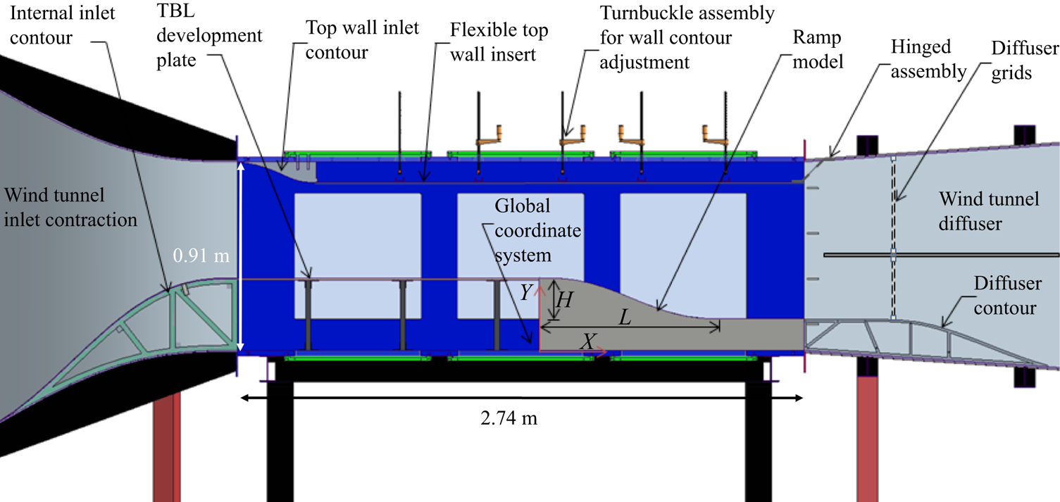
Figure 2. Schematic of the test section and model with key elements labelled.
On the top of the test section, a wall inlet contour smoothly transitions the flow from the inlet onto a flexible top wall insert. This flexible insert covers most of the test section and acts as an adjustable internal ceiling. It features two rows of turnbuckles that allow a continuous modification of the imposed streamwise pressure gradient. At the end of this flexible insert (which roughly corresponds to the end of the test section) is a hinge assembly that transitions the flexible ceiling into the diffuser and (1) provides rigidity to the design and (2) prevents feedback via the passage of flow above the flexible insert.
The experimental geometry was designed to provide initial two-dimensional, TBL growth under nominally zero pressure gradient conditions followed by the imposition of an adjustable APG that would be selected to achieve various extents of separated flow on the ramp.
The ramp geometry for these experiments is a fifth-order polynomial contour with zero first- and second-derivative end conditions. It is given by the following parametric form:
 \begin{equation}Y(X) = {a_1} + {a_2}{X^3} + {a_3}{X^4} + {a_4}{X^5},\end{equation}
where X denotes the streamwise distance from the end of the boundary layer development plate and Y(X) is the height of the ramp, both in the global coordinate system (see figure 2). The constants in (2.1) are given explicitly in terms of the ramp length, L = 0.9 m, the ramp height, H = 0.2 m (also shown in figure 2), and the vertical offset from the tunnel floor, Hoff = 0.152 m, as follows:
 \begin{equation}{a_1} = (H + {H_{off}}),\quad {a_2} ={-} 10H/{L^3},\quad {a_3} = 15H/{L^4},\quad {a_4} ={-} 6H/{L^5}.\end{equation}
A schematic of the ramp contour (without the offset Hoff) is depicted in figure 3.

Figure 3. Convex ramp model geometry (without the offset Hoff).
The ramp model is two-dimensional and extends the entire width of the test section. It was machined in-house from aluminium stock to a surface smoothness within 0.025 mm (0.001 in). Note that in addition to the contoured section of the ramp, there is a flat section of length 0.381 m (15.0 in) downstream of the ramp. Manufactured as part of the ramp model, this provides the flow with a recovery region prior to entering the wind tunnel diffuser. A photograph of the installed ramp model is shown in figure 4. This figure also highlights the global (X, Y, Z) and local (x, y, z) coordinate systems used in the study, and note that the y axis is locally normal to the ramp surface and the spanwise z axis is shared by both coordinate systems aligned with the ramp centre span.

Figure 4. Photograph of the test section model with wind tunnel sidewall door removed and the local and global coordinate systems highlighted.
2.2. Flow-field diagnostics
2.2.1. Static pressure measurements
In the experiments, it was exceedingly important to document the imposed streamwise pressure gradient on the convex ramp surface as well as its degree of two-dimensionality. To facilitate this, the convex ramp had a streamwise array of static pressure taps drilled locally orthogonal to the ramp surface, each with a diameter of 1.6 mm (0.063 in). The array contains 49 taps located at the ramp centrespan position. In addition, over a range of seven representative streamwise locations, spanwise arrays of five static pressure taps each allow the two-dimensionality of the imposed pressure gradient to be assessed. This, combined with 12 additional taps located on the upstream boundary layer development plate, yielded a total of 89 static taps. Static pressure measurements were acquired via a Scanivalve SSS-48C9 pneumatic scanner which houses a PDCR23D pressure transducer and an SCSG2 signal conditioner. This system has 48 pressure ports that can be measured sequentially using the internal pressure transducer, which has a differential range of 10 in of H2O (2490.8 Pa) with an accuracy of 0.30 % of full scale. Three Scanivalve 31-port circular quick connectors were used sequentially to measure surface static pressure from the 89 pressure taps along the ramp and boundary layer development plate. The channels were sampled sequentially at 1 kHz and pressure data are reported as a pressure coefficient defined as follows:  ${C_p} = ({P_i} - {P_\infty })/({P_o} - {P_\infty })$, where Pi is the local wall static pressure, Po is the free-stream stagnation pressure and P∞ is the free-stream static pressure. The reference pressure for each measurement was the free-stream static pressure collected via a Pitot-static tube located at X = −0.97 m, Y = 0.58 m and Z = 0.19 m.
2.2.2. Velocity measurements
With the exception of constant-temperature hot-wire surveys of the TBL upstream of the ramp, velocity measurements were performed using laser Doppler velocimetry. These were collected using a two-component Dantec Dynamics Fiber Flow System featuring a BSA F60 Flow processor and BSA Flow Version 6.5 software. The system was operated in 180° backscatter mode and a Bragg cell was used to unambiguously detect flow direction. Two different focal length lenses were used on the two-dimensional 60 mm fibre optic probe head. A 600 mm focal length lens was used for all profiles taken on the centrespan location. For many of the off-span profiles, a 400 mm focal length lens was utilized for its ability to yield higher data rates. The probe measurement volume has a maximum wall-normal dimension of 0.38 mm (0.015 in) which sets the effective spatial resolution of the measurements. Particle seeding was injected into the boundary layer at select spanwise locations via the lower internal inlet contour in the wind tunnel inlet contraction. The seed particles consisted of diethylhexyl sebacate and utilized a TSI Six-Jet Atomizer 9306 high-volume liquid droplet seeding generator to achieve particles of nominally 1 μm in diameter.
2.2.3. Surface flow visualization
As described in Merzkirch (Reference Merzkirch1987), there exist several approaches to surface flow visualization. One of the classic methods is that of oil-film flow visualization. Here the objective is to visualize the skin-friction lines on the surface. Lu (Reference Lu2010) noted that it is difficult to suggest a single method since facilities and applications are so varied. The approach used in this study was inspired, in part, by a recently developed method from NASA Langley Research Center as reported by Koklu & Owens (Reference Koklu and Owens2017) which used aviation oil, kerosene and nanosized silica particles. The surface mixture used in the work reported here consists of: (67 %) kerosene, (20 %) w100 aviation oil, (12 %) titanium dioxide and (1 %) oleic acid all combined by weight and applied to the surface via lightly brushing. Aviation oil fluoresces under ultraviolet (UV) light, leaving luminous flow patterns on the surface. It was found that titanium dioxide, with the addition of oleic acid to prevent clumping, aids the aviation oil in enhancing the surface skin-friction lines. The basic idea is that when a light coating of the mixture is applied to the surface and a flow-induced shear is applied, via running the wind tunnel, the kerosene acts as a carrier agent and allows the aviation oil and titanium dioxide to flow along the surface. The air flow promotes the evaporation of kerosene and after an extended period of time, O(30–60 min), most of it has evaporated leaving behind the titanium dioxide powder and aviation oil. Since the layer of oil on the surface is extremely thin, it retains the surface flow pattern with plenty of time to stop the tunnel, apply a UV light and photograph the results.
3. The large-scale flow separation case
Several ceiling configurations were examined and the one selected to yield a large-scale separation that forms the focus of this paper is shown in figure 5. Also shown are the corresponding streamwise pressure coefficient and pressure coefficient gradient distributions. The pressure gradient is initially mildly favourable due to the upper ceiling contour at the test section inlet, followed by a region of nominally zero pressure gradient on the plate upstream of the ramp. The location X = −0.56 m was chosen as the initial condition, and velocity profiles taken there using constant-temperature anemometry showed both spanwise uniformity and canonical zero pressure gradient TBL characteristics. There is a favourable pressure gradient near the ramp leading edge, followed by a strong APG commencing near X = 0.2 m. In terms of the Clauser parameter,  $({\delta ^\ast }/{\tau _w})\,\textrm{d}{P_\infty }/\textrm{d}x$, the flow is highly non-equilibrium. For example, on the boundary layer development plate upstream of the ramp $\beta ={-} 0.03$ while near the leading edge of the ramp, X = −0.04 m, $\beta ={-} 1.07$ due to the flow acceleration suggested in figure 5. On the ramp itself, $\beta > 1$ upstream of TBL separation.

Figure 5. (a) Ceiling configuration and (b) streamwise pressure coefficient and pressure coefficient gradient for the large-scale separation case.
Figure 6(a) presents outer-variable-scaled mean velocity profiles at X = −0.56 m, demonstrating the spanwise uniformity of the TBL upstream of the ramp. The centrespan mean velocity profile in figure 6(b) shows the classic logarithmic law of the wall behaviour for approximately 30 < y + <700. Both the Clauser method and oil-film interferometry were used to determine the upstream local wall shear stress for inner-variable scaling. Table 1 summarizes the TBL parameters at X = −0.56 m.

Figure 6. (a) Outer-variable-scaled mean velocity at X = −0.56 and (b) inner-variable-scaled mean velocity at the centrespan location (the red line denotes logarithmic law of the wall).
Table 1. The TBL parameters upstream of the ramp.
The spanwise variation in static pressure was measured at seven selected streamwise locations on and just downstream of the ramp. At each of these locations five pressure taps covering approximately the central 40 % of the span were used to record and analyse the uniformity of the flow. If any significant spanwise variation in pressure was observed, the side-to-side flexible ceiling positioning was adjusted to eliminate this behaviour. Figure 7 shows the spanwise pressure distribution for the large-scale flow separation case and indicates that there was no significant spanwise pressure gradient. While the spanwise static pressure uniformity does not in any way imply two-dimensional flow, it does indicate that the upper flexible tunnel ceiling was properly oriented in the spanwise direction.

Figure 7. Spanwise variation of static pressure on and downstream of the ramp (central 40 % of the tunnel span).
The streamwise evolution of the mean flow at three spanwise locations is shown in figure 8. All the profiles were taken via laser Doppler velocimetry measurements in the local wall-normal coordinate y (see figure 4) and are referred to by their starting streamwise, X, wall location. The centrespan profiles (z = 0) are marked with blue diamonds, the mid-span profiles (z = −0.13 m) with black circles and the near-sidewall profiles (z = −0.26 m) with green triangles. Initially, over the boundary layer development plate, the profiles exhibit a shape factor  $(H \equiv {\delta ^\ast }/\theta )$ typical of zero pressure gradient TBLs, $H \approx 1.3- 1.4$, and are quite uniform in spanwise extent. Along the ramp, however, three-dimensionality of the flow starts to become evident with the spanwise variation in the mean velocity profiles. The first noticeable spanwise deviation in the profiles commences near X = 0.1 m with the centre profile showing signs of acceleration greater than that of the off-centre profiles. Between X = 0.2 m and X = 0.3 m, the pressure gradient becomes adverse and the signs of a spanwise variation in the mean flow become more readily apparent. From this X value onward, the off-centre profiles have a progressively larger velocity deficit, compared to the centreline profile. Around X ≈ 0.45 m, the flow closest to the tunnel sidewall separates, in the mean sense, followed by the middle profile and the centre profile by X ≈ 0.55 m. Shape factor H begins to grow at X = 0.3 m until separation occurs, at X = 0.45–0.55 m, where H varies from H = 2.5 to 3.0. Interestingly, each of these values is individually in good agreement with intermittent transitory detachment separation values of H sep 2.76 ± 0.23 reported by Castillo, Wang & George (Reference Castillo, Wang and George2004).

Figure 8. Streamwise evolution of locally wall-normal profiles of mean velocity starting from the boundary layer development plate, X = −0.56 m, and continuing along the ramp through separation, reattachment and recovery at X = 0.95 m.
The approximate separation and reattachment locations, as inferred from the sequence of mean velocity profiles like those shown in figure 8, are shown in table 2. Spanwise variations in the separation location range from X = 0.53 m to X = 0.44 m while variations in the reattachment location range from X = 0.83 m to X = 0.84 m. In terms of a percentage of the total ramp length (L = 0.9 m) over the spanwise region measured, the variation in separation location was 10 % of the ramp length whereas the spanwise variation in reattachment location was only approximately 1 % of the ramp length. The extent of the streamwise separation region ranged from 33 % to 44 % with the mean extent over this span being 39 % of the ramp length.
Table 2. Approximate separation and reattachment locations, and the streamwise extent of the separation, at three spanwise locations.

From figure 8 it is apparent that, despite the spanwise uniform approach flow and fully two-dimensional ramp geometry, the flow separation is three-dimensional. This has been observed in many previous studies involving fully two-dimensional geometries but is typically not considered in detail. Often the separation is treated as quasi-two-dimensional or the focus is on separation control strategies. It is this three-dimensionality of the flow separation that forms a focal point of this paper. Note also that the extent of the flow three-dimensionality is not confined to the near-wall region.
4. Flow separation topography
In this section, the topography of the surface flow pattern for large-scale separation on the ramp is described. The surface flow topography is the surface flow pattern observed over the ramp using the fluorescent oil-film flow visualization technique previously described. It presents the relationship between surface flow features, including their respective sizes and positions. Our approach follows Legendre's (Reference Legendre1956) postulate that streamline patterns adjacent to a surface have properties consistent with a continuous vector field. Only one trajectory passes through each regular point. Furthermore, singular points of the field can be categorized mathematically. Flow features in the form of singular points (or critical points) are identified throughout these images as they are used in a following section to construct surface flow topological maps of the separation and reattachment regions. The taxonomy of the associated flow separation topology is shown to be ubiquitous and follows that characterized by Perry & Hornung (Reference Perry and Hornung1984) and Chong & Perry (Reference Chong and Perry1987). As noted by those authors, the patterns are created by vorticity departing from the wall and carried into the free stream. Isolated singular points are those locations where the subject vector is zero and the direction is undefined. There are two primary types of singular points: the node (N) and saddle (S) points, with the node also taking the form of a focus (F) or centre (C). Any of these generic singular points can take on an attachment or separation form. For example, a node of separation or attachment would behave as a sink or source, respectively, thus differing in the sign of the flow direction along the surface.
A saddle point acts to separate the skin-friction lines that issue from adjacent nodal points of attachment. Lighthill (Reference Lighthill1963) describes the existence of a saddle point from which a line emerges that separates the streamline pattern into two families as a necessary condition for a line of separation. Lighthill (Reference Lighthill1963) also argues that limiting streamlines near a line of separation must leave the surface rapidly. In what follows we take the term ‘separation’ to be synonymous with ‘flow detachment’ from the surface. It is also worth clarifying that topology primarily differs from topography in that while the topography is concerned with the flow features, including size, strength and their respective locations to one another, topology is only concerned with the connections between these features.
At the outset, it should be noted that multiple experimental trials were performed and the resulting flow patterns were found to be highly repeatable between experimental runs. Hence, the flow visualization images and associated surface flow topography described in this section may be considered representative of those encountered over multiple trials. Also, the surface flow visualization provides details of the time-mean, near-wall flow pattern but not its unsteadiness.
The global surface flow visualization of the ramp, consisting of the pattern of skin-friction lines, is presented in figure 9. The wind tunnel sidewalls are at the edges of the lighter blue oil visualization on the ramp surface in the figure. As originally described by Legendre (Reference Legendre1956), these skin-friction lines are the limit of the streamlines as the flow approaches the surface and, as such, have the characteristic that the flow must be locally tangent to them. Each unique, regular point on the surface lies on one skin-friction line and follows one distinct trajectory. In three-dimensional flow fields, the local wall shear stress vector has two components. The two components are both uniquely zero at singular points.

Figure 9. Surface flow visualization of the ramp flow with four interrogation regions highlighted. Incoming flow is from right to left.
The surface flow pattern shown in figure 9 is clearly dominated by the presence of two large, symmetric, counter-rotating vortical structures in the central region of the ramp, and a spanwise uniform reattachment farther downstream; together these features extend over nearly 50 % of the ramp surface. Here the term vortical structure equates to a topological singular point of a focus (an inward- or outward-spiralling node). Despite the spanwise uniform approach flow and the two-dimensional ramp geometry, the surface flow pattern indicates an inherently three-dimensional flow field above the majority of the ramp. Over the ramp, the APG, model finite span and wall curvature morph the flow field into a complex three-dimensional structure that exhibits a considerable degree of side-to-side symmetry with respect to the ramp centre plane. Hence, describing the ramp flow separation in terms of two space variables, while simplifying, is clearly inappropriate.
Due to the large spatial extent of the ramp and the detailed surface flow features to be examined, four interrogation regions indicated in figure 9 are explored in detail before a global analysis of the entire ramp surface is presented.
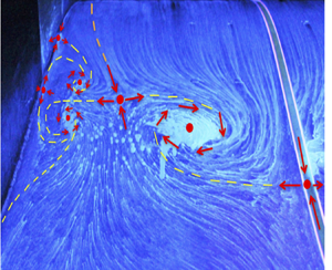
View 1 of figure 9 is highlighted in figure 10, showing the surface details of the separation structure and surrounding smaller-scale flow topography on the far side of the ramp surface (corresponding to the inner loop side of the wind tunnel). The flow is from top to bottom. There are two prominent saddle points. Along the centreline of the ramp, fluid is drawn towards saddle point 1, whereas the fluid nearer the sidewall is drawn towards saddle point 3. Both saddle points then divert fluid into the central focus 2, where the flow must lift off of the surface to satisfy the Helmholtz circulation theorem (Batchelor Reference Batchelor1967). The line dividing the upstream region from the downstream region – shown as the yellow dashed line in figure 10 – is the line of separation. This line of separation forms the base of the stream surface, which is called a dividing surface (Tobak & Peake Reference Tobak and Peake1982), where the flow detaches from the ramp. This dividing surface extends both into the flow and downstream.

Figure 10. View 1 from figure 9; the yellow dashed line is the line of separation; the orange dashed line shows how the near-sidewall flow is directed towards the central flow separation. Flow is from top to bottom.
Nearer the tunnel sidewall, there are a number of smaller-scale features (also connected to the dividing surface just mentioned). Two appear to be the counter-rotating foci, denoted F4 and F5, which are bounded by two saddle points, denoted S6 and S7, which are located very near the tunnel sidewall. The farthest upstream saddle point, S6, is the source of the sidewall separation. The extent of its effect is limited by S3 as the skin-friction lines away from the sidewall are diverted back and around F4.
View 2 of figure 9 is shown in figure 11 and presents the separation topography on the opposite side of the ramp corresponding to the wind tunnel outer loop. Comparison with figure 10 shows that the centreline symmetry of the two foci F2 and F12 is very high. From images taken on both sides of the tunnel centre span it is apparent that the sidewall separation saddle points S6 (in figure 10) and S16 (in figure 11) direct the flow towards saddle points S3 and S13, respectively. Hence, from a skin-friction line point of view, the sidewall flow separation does not directly cause the central separation structures. Instead, any direct influence the sidewall boundary layers have on the central vortical structures is limited to the area farther upstream, prior to the location where separation occurs. While sidewall separation does not directly give rise to the central vortical structures, figures 10 and 11 clearly show that it is associated with centrespan-directed fluid motion consistent with the rotation of the central vortices.

Figure 11. View 2 from figure 9; the yellow dashed line is the line of separation; the orange dashed line shows how the near-sidewall flow is directed towards the central flow separation. Flow is from top to bottom.
The reattachment region, which is highlighted in views 3 and 4 of figure 9, is shown in figure 12. While the separation initiation is obviously not spanwise uniform, in contrast the reattachment is. This is highlighted by the red dashed line. Central reattachment initiates at node N22, which acts as a source, feeding in all directions with an almost pure cross-flow component along the reattachment line. Just upstream or downstream of this line there is still a major cross-flow component that appears to vary only slightly with spanwise location, indicating some limited degree of three-dimensionality. Near the tunnel side wall, the cross-flow component changes direction. In this region are identified saddle point S21 and nodal point N20. N20 feeds into S21 as well as into the upstream focus F15. Due to the virtually perfect symmetry, the inner tunnel wall reattachment topography is not presented here.

Figure 12. Close-up views of the reattachment in the central ramp region (view 4) and near the wind tunnel outer loop sidewall (view 3). Incoming flow in view 4 is from right to left and for view 3 from bottom to top.
In order to further emphasize the degree of spanwise uniformity of the flow reattachment, figure 13 shows the result of surface flow visualization in which oil that illuminates blue under UV lighting was placed in the expected region of separated flow and an oil solution that illuminates green under UV light was placed just downstream of the expected reattachment region. After approximately an hour of run time, the flow was stopped and the results photographed. Remarkably, there is virtually no mixing of the two solutions, thereby indicating the temporal stability of the flow reattachment pattern. Where the blue dye is placed, almost all the flow is reversed – a characteristic of the separation region. In contrast, where the green dye is placed, all the flow is directed downstream, characteristic of attached flow. The only region where mixing occurs is on the far side in the image where the reattachment line is positioned slightly upstream from where the blue dye was first placed and hence the fluid diverted by saddle point S21 can be clearly seen heading downstream. The mixing of the blue dye near S21 shows just how much surface movement in the fluid occurs. Furthermore, this mixing is only apparent since the blue dye was initially applied just downstream of the reattachment line, highlighting just how remarkably spanwise uniform the reattached flow is.

Figure 13. Two-dimensionality and temporal stability of the reattachment region, captured using two different UV illuminating surface flow solutions. Incoming flow is from left to right in both images.
Surface flow visualization was also conducted on each tunnel sidewall in order to individually capture the associated topography there. Close-up photographs were taken in situ, as well as with the tunnel window insert removed. Figure 14 shows the surface flow visualization on the wind tunnel outer loop sidewall and highlights the character of both the sidewall juncture flow separation and sidewall reattachment. Figure 14(b) shows the initial stages of separation from the sidewall juncture which initiates from saddle point S16 (as shown previously in figure 11) and terminates into focus F14. It is likely that in the flow above the surface, F14 and F18 are connected by the same stream surface spiralling into their cores. In essence, one vortex curves and impinges on the surface leaving ‘footprints’, F14 and F18, on the ramp and sidewall. Saddle point S17, which is not visible in figure 11, is located on the sidewall. It is connected to F14 – determined via flow visualization experiments not presented here. Figure 14(c) highlights the reattachment region. The reattachment line on the surface of the ramp passes through N20, as also seen in figure 12, and then leads up the sidewall surface into saddle point S19. A close look reveals many reattached source lines leaving node N20 and heading upstream before being diverted back downstream in the vicinity of S19. This saddle point is the last singular point in the reattachment line and divides the separated fluid, which is directed upstream into F15 (see figure 11) from the reattached fluid.

Figure 14. (a) Visualization on the ramp surface and wind tunnel outer loop sidewall, (b) with close-up views highlighting the sidewall juncture flow separation and (c) sidewall reattachment. Flow is from left to right in all images.
It is important to address the question of how common is the previously described surface flow separation pattern? One of the most widespread smooth body backward-facing ramp geometries is the Stratford ramp originally proposed by Stratford (Reference Stratford1959a,Reference Stratfordb). Previous work conducted on the Stratford ramp geometry (which is similar to the geometry used here) has yielded remarkably similar surface flow patterns in studies by Koklu & Owens (Reference Koklu and Owens2017) and Koklu (Reference Koklu2018). Figure 15 shows the two-dimensional ramp geometry used by Koklu and the resulting baseline surface flow separation and reattachment patterns. The similarity to the flow separation pattern observed in this study is apparent. Every work tied to the Stratford ramp concept, both experimental (e.g. Stratford Reference Stratford1959a,Reference Stratfordb; Elsberry et al. Reference Elsberry, Loeffler, Zhou and Wygnanski2000; Kumar & Alvi Reference Kumar and Alvi2006, Reference Kumar and Alvi2009) and computational (e.g. Zhang & Fasel Reference Zhang and Fasel1999; Fasel, Gross & Postl Reference Fasel, Gross and Postl2001), has reported a related form of flow separation three-dimensionality. However, the type of three-dimensional flow separation observed in our study is not limited only to Stratford-type ramp geometries. Other non-Stratford ramp geometries feature similar separation characteristics. These include the smooth but steeper backward-facing ramp geometry studied by Gardarin & Jacquin (Reference Gardarin and Jacquin2009), a two-dimensional bump with leeward separation studied by IMP, Gdansk, as described in Délery (Reference Délery2013) and serpentine inlet ducts, or S-ducts, studied by Anderson, Reddy & Kapoor (Reference Anderson, Reddy and Kapoor1994). Many researchers have noted central vortical flow patterns similar to those shown in figure 9 and have likened them to secondary flow and vortex lift-off in a duct, but few have considered the matter further. While the central vortical patterns are important due to their prominence in the region of measurement, the previously presented images show that there are many other topological features, i.e. singular points, which make up the surface flow pattern and these have not been previously noted or discussed. Investigating these features, and their connections to one another, provides clues as to why the patterns form and insight regarding their inherent sensitivity.

Figure 15. (a) Ramp geometry and (b) ramp surface flow visualization pattern (taken from Koklu Reference Koklu2018).
It has been common to try to produce a two-dimensional flow separation for experimental study because it simplifies the problem. However, for smooth body backward-facing ramp geometries this ‘two-dimensionality’ is, as demonstrated above, the exception and not the rule. To examine this aspect further, Simmons (Reference Simmons2020) compared the ramp geometries from both the current and eight previous smooth body flow separation experiments including those previously cited. With the exception of the rounded backward-facing step of Lin (Reference Lin1992), all the geometries are remarkably similar, possessing an initial region of convex surface curvature followed by concave curvature. Other than the similar two-dimensional profile of the geometries, the main defining physical feature exhibited by these studies is the aspect ratio, or the ratio of the ramp length (L) to width (W) to height (H) and these are tabulated in Simmons (Reference Simmons2020). Most of the geometries had similar aspect ratios of L/H ~ 3–5 (L/H = 4.5 in the current study). The ratio of length to height (L/H) has a significant impact on the streamwise pressure gradient, influencing the occurrence and extent of flow separation.
One might expect the ramp length-to-width ratio (L/W) to affect the degree of spanwise uniformity of the flow separation. If  $L/W \ll 1$, the flow might be expected to be relatively uniform, with the secondary flow effects confined to regions near the sidewall. However, when L/W ~ 1 it is expected that the flow will exhibit a significant region of three-dimensionality. Of the geometries used, most fall in the range of $L/W\sim 1$ ( $L/W = 0.98$ in the current study). Exceptions were the studies by Debien et al. (Reference Debien, Aubrun, Mazellier and Kourta2014) and Lin (Reference Lin1992), whose values of $L/W = 0.24$ and 0.176, respectively, were due to a uniquely wide, 2 m, test section and a comparatively small ramp length, respectively. It is interesting to note that these two studies did not mention three-dimensional effects and the flows were treated in terms of two-dimensional terminology.
In an effort to examine whether the extent of the flow separation topography scales with the ramp aspect ratio L/W, three-dimensional RANS simulations were conducted by Wang & Zhou (Reference Uzun and Malik2018) and the results are presented in Simmons (Reference Simmons2020). The simulations utilized the SA-RC turbulence model and were conducted on three different scaled versions of the ND ramp, all having the same streamwise pressure gradient at corresponding streamwise positions. The scaling was such that the L/H ratio was fixed at 4.5 (as in the current experiment) and three geometrically identical ramps of different heights, H, H/2 and H/4, were simulated. In effect, reduction in H increases the relative spanwise width of the ramp and reduces L/W. The three-dimensional simulations show twin central vortical separation structures qualitatively similar to those observed in the current experiment. The results show that as L/W decreases the vortical structures move closer to the sidewall, thereby extending the central region of uniform flow. This provides supporting evidence that to achieve a spanwise uniform flow, the width of the ramp must be significantly longer than its length,  $L/W \ll 1$. Perhaps most importantly the results show that while the relative uniformity of the flow scales with the aspect ratio of the geometry, they do not suggest that the flow ever becomes two- dimensional. In fact, it appears that the primary separation structure does not depend on the ramp aspect ratio, but instead remains relatively unchanged with only its location and size altered.
5. Flow separation topology
Having documented the surface flow topography, attention is next given to the corresponding flow topology – the underlying structure of the flow separation. Topology primarily differs from topography in that, while topography is concerned with the flow features, including their size, strength and location(s) with respect to one another, topology is only concerned with the connections between these features. Topology follows a set of rules that constrain the reconstruction of the surface flow patterns and clarify the possible connections between singular points.
Using the information gleaned from the topographical images presented in the previous section, a picture of the global flow topology can be created. Every effort has been made to accurately capture all the flow features and their singular points. As Hunt et al. (Reference Hunt, Abell, Peterka and Woo1978) note, ‘one of the main reasons for classifying the zero-shear-stress or singular points in topological terms as nodes and saddle points is because there is a relation between the number of nodes and the number [of] saddles’. This relation, which comes from the Poincaré–Bendixson theorem (e.g. Tobak & Peake Reference Tobak and Peake1982; Hunt et al. Reference Hunt, Abell, Peterka and Woo1978), takes many forms with the most common being
 \begin{equation}{\varSigma _{nodes}} - {\varSigma _{saddles}} = 2.\end{equation}
Equation (5.1) applies to an isolated body without holes or handles. Its Euler characteristic is 2 as is the sum of the indices of its singular points. It is colloquially known simply as the summation rule and states that there must be two more nodes than saddle points. Perhaps a more useful form of the summation rule is derived when (5.1) is modified for a three-dimensional body (designated B) and plane surface (designated P) in a wind tunnel. This occurs by treating the upstream flow as emanating from a source and the downstream flow as terminating in a sink. When this source and sink are accounted for, the following form is reached:
 \begin{equation}{[{\varSigma _{nodes}} - {\varSigma _{saddles}}]_{P + B}} = 0.\end{equation}
Here the body (B) represents the given flow-field geometry, which is connected to the wind tunnel interior walls, the plane surface (P). This is the form commonly used in wind tunnel surface flows and states that the number of saddle points must equal the number of nodes.
Care should be taken when using these equations to validate a possible flow field. Because complete isolation of the body is rare, wind tunnel experiments must account for the model, support, test section walls, etc., as noted by Délery (Reference Délery2013). In the flow of interest here, if it is assumed that all of the singular points occur on the ramp surface and adjacent wind tunnel sidewalls, and any other singular points occur in offsetting pairs (a reasonable assumption), then (5.2) and (5.3) can be readily applied. If the equation is satisfied, the map is a possible solution to the flow field. If it does not hold, there is an error in either the identified singular points or their connectivity, or there is missing information. Satisfying (5.2) and (5.3) indicates that the proposed map is a mathematically viable portrayal of the flow. In other words, while satisfying the summation rule does not confirm the flow pattern, it quickly rules out numerous erroneous patterns, and this is its primary utility. Note that an alternative approach of obtaining the appropriate topological constraint for the problem is that described in Foss (Reference Foss2004) and Foss et al. (Reference Foss, Hedden, Baros and Christensen2016).
5.1. Surface flow topology
In order to create a topological map, the entire surface flow field was carefully inspected, and the flow features and their singular points were identified as described in § 4. This was then checked against (5.2) to ensure that a valid number of singular points were identified. Subsequently, a connection between singular points was proposed that agreed with the surface flow visualization pattern including the consistency of flow direction in the vicinity of singular points. Once a valid map was proposed, it was checked with additional surface flow visualization trials and close-up inspection of the singular points. This process was iterated until a satisfactory solution was reached. The resulting topological map is shown in figure 16. It contains 22 identifiable singular points on the ramp and sidewall surfaces: 11 nodes and 11 saddle points.

Figure 16. Topological map (phase portrait) of the flow for the large-scale separation case, drawn to scale based on the flow-field topography presented in the previous section.
The map's orientation is such that the top corresponds to the leading edge of the ramp while the ramp trailing edge is located at the bottom. The map in figure 16 spans part way up both wind tunnel sidewalls. For ease of comparison with the previously presented topographical images, the map is drawn roughly to the scale of the flow features. Note that while the topology is symmetric about the tunnel centreline, the topography of some of the flow features near the sidewalls varies slightly from run to run; to represent this variation, some of the singular points at these locations are not presented in a purely centreline-symmetric fashion. The topological map shown in figure 16 provides a visual interpretation of the overall surface flow that previously was only available in fragmentary pieces in the surface flow visualization photographic images.
Topological analysis can also serve to provide a qualitative understanding of the character of the off-surface flow field. Hunt et al. (Reference Hunt, Abell, Peterka and Woo1978) developed a form of the summation rule that can be applied to streamlines via planar slices of the flow. For a two-dimensional streamwise or cross-sectional slice, singly connected, (5.2) takes the form
 \begin{equation}[{\varSigma _{nodes}} + {\textstyle{1 \over 2}}{\varSigma _{N\mathrm{^{\prime}}}}] - [{\varSigma _{saddles}} + {\textstyle{1 \over 2}}{\varSigma _{S^{\prime}}}] = 0,\end{equation}
where nodes include foci, N′ indicates half-nodes and S′ half-saddle points bound with a surface. This approach as applied to flow around surface-mounted obstacles is presented in Hunt et al. (Reference Hunt, Abell, Peterka and Woo1978). As noted by Dallmann (Reference Dallmann1985), while there is no unique relationship between the surface flow pattern and the topology of the entire three-dimensional flow, some off-surface flow information can be inferred from the skin-friction patterns. One such example here is the flow along the tunnel centreline plane that includes separation saddle point S1 and reattachment node N22, both of which are shown in figure 16. Chapman & Yates (Reference Chapman and Yates1991) point out that whenever a saddle point and node of opposite type are formed from a bifurcation (as is the case here), an isolated singular point appears in the flow above the surface.
This singular point is depicted as focus F27 in figure 17, which also shows a qualitative rendering of streamlines taken in a wall-normal plane along the ramp centreline. Here the fluid separates at S1 and wraps around the newly discussed singular point, F27. Downstream from this point, the fluid reattaches at N22. In figure 17, S1 and N22 are the same singular points identified in the surface topology shown in figure 16; however, along this plane they are both half-saddle points. The ‘half’ distinction is due to their being joined with the ramp surface, while node N22 is technically a saddle point since flow enters on one axis (the free stream) and departs along another (the ramp surface). This topology satisfies the summation rule (equation (5.3)) for a streamwise slice with two half-saddle points and one node in the form of a focus. While the formation of a centre instead of a focus is possible, this is not likely here, as it is a singular case rooted in the limit of two- dimensional separation – an example of an unstable saddle-point-to-saddle-point connection. As for stability, F27 must be stable and spiral inward as drawn in figure 17. Physically, it consists of spanwise vorticity, created by the shearing at the wall. The flow, separating from the surface via S1, travels along an inward-spiralling plane and orthogonally out through the vortex core, F27.

Figure 17. Streamwise slice of the centreline flow topology.
5.2. The owl-face pattern
The qualitative similarity between the surface flow patterns in both the current and prior experiments was discussed in § 4 with emphasis placed on the flow topography. Here we show that the topological structure is even more ubiquitous. The core topological structure in figure 16 is the connection of S1–F2–S3–N22 and its symmetric side S1–F12–S13–N22. This forms a recognizable pattern known as an ‘owl-face pattern (OFP) of the fourth kind’. There are at least four types of OFPs which are described in Perry & Hornung (Reference Perry and Hornung1984) and these are reproduced in figure 18. They note that these patterns are created by vorticity departing from the wall and being carried into the free stream. Since the vorticity is concentrated along the core, they claim that these OFPs can be generated via Biot–Savart induction by the vortex cores. Chong & Perry (Reference Chong and Perry1987) later numerically generated many of these OFPs using local Taylor series expansion solutions of the Navier–Stokes equations. The OFP was first identified by Fairlie (Reference Fairlie1980); they are ubiquitous in flows over both two- and three-dimensional geometries. Fairlie (Reference Fairlie1980) notes that the OFP, or some variation thereof, appears in flows from many different physical geometries ranging from bodies of revolution at incidence (Fairlie's own work), to nominally two-dimensional airfoils, shallow bell-shaped hills and nominally two-dimensional diffusers (the case investigated here) and ‘seems to be one of the most commonly occurring structures to be found in three-dimensional separations’. While many authors have recognized OFPs in their own work, few have tried to explain why these patterns form so frequently. What follows is an attempt to clarify this aspect.

Figure 18. Topological structures of OFPs of the first (a), second (b), third (c) and fourth (d) kinds as defined by Perry & Hornung (Reference Perry and Hornung1984).
Since a topological map is only concerned with the connections between features, not their locations relative to one another, the topological map shown in figure 16 can be drawn in a manner that is easier to visually interpret. Figure 19(a) presents the same topological map, but simplified to highlight the distinct separation and reattachment structures. This is equivalent to taking the map of figure 16, unfolding and stretching it while fully maintaining all the connections between flow features. In other words, the topology of figure 19(a) is identical to that of figure 16. Only the topography has been changed. The figure clearly presents a repeating pattern of saddle points and foci for separation, as well as nodes and saddle points for reattachment. This repeating pattern, regardless of the number of saddle–focus and node–saddle pairs, represents a generalized OFP. In particular, the OFP of the fourth kind noted by Perry & Hornung (Reference Perry and Hornung1984) can be identified in figure 19(a) as the grouping of S1–F2–S3–N22 and its symmetric side S1–F12–S13–N22. What is really striking about the topological map in figure 19(a) is that the global line of separation can be neatly unravelled in such a simple manner. Thus, although the surface separation pattern is far from spanwise uniform, its core topological structure is not complex.
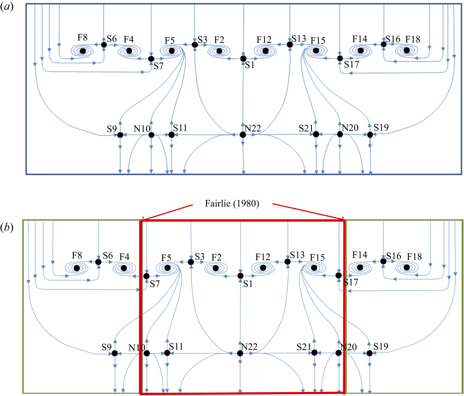
Figure 19. (a) An equivalent redrawing of the topological map in figure 16 highlighting the repeating separation and reattachment regions which together form a ‘generalized OFP’. (b) The ramp surface flow topology map with the common topology of the Fairlie (Reference Fairlie1980) spheroid at angle of incidence highlighted.
The OFPs do not always occur as the isolated structures defined by Perry & Hornung (Reference Perry and Hornung1984). Re-examining the work of Fairlie (Reference Fairlie1980) in which the OFP was first identified provides an example of this. The topology provided by Fairlie (Reference Fairlie1980) is sketched in figure 20(a). This highlights the flow patterns observed on a prolate spheroid at 5° angle of incidence. One can identify OFPs of both the first (flank) and fourth (leeward and windward) kinds. Figure 20(b) depicts the synthesized version of the topology, where the top and bottom saddle–node pairs are the same and are repeated for clarity.

Figure 20. (a) Topology sketch based on Fairlie's (Reference Fairlie1980) flow visualization and (b) synthesized topology of the surface flow over the prolate spheroid at 5° angle of attack.
Just as the OFP observed in Fairlie's (Reference Fairlie1980) study was part of a larger structure, the OFP of the fourth kind observed in the current investigation is also part of the larger structure shown in figure 19(a) which has been labelled the generalized OFP. Figure 19(b) shows that the topology observed in Fairlie's (Reference Fairlie1980) work (highlighted by the red box) is also contained within the structure of the generalized OFP observed for the ramp flow investigated here. That is, S7–N10 and S17–N20 of figure 19(a) correspond to the top/bottom saddle–node pair shown in figure 20. The extra saddle–focus pairs and corresponding nodes on the ramp surface are a result of the tunnel sidewall boundary condition, whereas the central structures that are common to both the ramp and spheroid must be purely a result of the remaining driving forces: pressure gradient and surface curvature.
This stems from the fact that Fairlie's work was conducted on bodies of revolution at incidence, hence no sidewalls were present; only surface curvature and pressure gradient effects influenced the surface flow patterns.
What it is important to note about the experimental study by Fairlie (Reference Fairlie1980) is that the angle of incidence yielded azimuthally asymmetric flow conditions, even though the geometry was axisymmetric. In addition to the streamwise APG, there was also a spanwise pressure gradient driving a cross-flow and the three- dimensional separation via the OFPs.
The generalized three-dimensional separation structure previously presented provides the form that separation takes. However, this is a repeating pattern, so it does not describe the exact number of ‘links in the separation chain’. For example, in the flow over Fairlie's spheroid, four foci and four saddle points made up the separation line (see figure 20), while in the smooth body ramp flow under consideration here, eight foci and seven saddle points were connected to form the separation lines (see figure 19). Of course, other combinations of saddle–focus pairs are also topologically possible.
The common flow topology of the current experiment and that of the spheroid at incidence of Fairlie (Reference Fairlie1980) suggests the importance of the combined influence of APG and a secondary flow. In the case of the spheroid, the secondary flow is generated due to the incidence angle. In the ramp experiment, it is in large part associated with the sidewall separation. Separation at the sidewall–surface junction is well recognized. The presence of the sidewall boundary layers, in conjunction with the ramp boundary layer, provides a momentum deficit that will naturally lead to flow separation provided a sufficient streamwise APG exists. Additionally, a spanwise pressure variation with higher pressure near the sidewalls and lower pressure near the tunnel centreline can also be expected due to the momentum deficit and earlier separation at the sidewall–ramp junction. This will serve to produce a significant spanwise flow component as is apparent from figures 10 and 11. Thus, the imposed pressure gradient in combination with the ramp–sidewall flow condition is consistent with formation of the central flow separation topology.
Key to the formation of the central vortical separation structures F2 and F12 is the combination of the upstream flow separation at saddle points S3 and S13 and the centrally located saddle point S1 farther downstream. Together, these give rise to spanwise flow consistent with the direction of rotation of the central foci F2 and F12. Saddle points S3 and S13, in turn, are intimately related to the sidewall separation. Figure 16 shows that sidewall separation initiates at saddle points S6 and S16 near the inner and outer walls of the tunnel, respectively. Associated pairs of foci F8 and F4 near the inner wall and F14 and F18 near the outer wall are ‘footprints’ of the associated corner vorticity that develops as a consequence of this separation. These features are located upstream of the central flow separation, S1. Saddle points S3 and S13 are, in turn, associated with the two counter-rotating foci pairs F4, F5 and F14, F15, respectively. These draw fluid towards the wall and further exacerbate the propensity of the ramp flow to separate via S3 and S13 upstream of the centreline. Consistent with this scenario, the three-dimensional RANS simulations of Wang & Zhou (private communication, 2018) show that the central vortical separation structures persist as the ramp is widened (i.e. as L/W is reduced at fixed L/H) but move closer to the sidewalls as the ramp is widened such that the central separation becomes more spanwise uniform.
6. Conclusion
Fluorescent surface oil-film flow visualization experiments demonstrate that, despite both a fully two-dimensional ramp geometry of finite span and spanwise-uniform approach TBL, the resulting flow separation over the ramp is inherently three-dimensional and appears dominated by two spanwise-symmetric, counter-rotating vortical structures. It is also shown that, while this type of flow separation appears to be quite common for smooth, backward-facing ramp geometries with length-to-width ratios of order 1, there has been very little documentation or characterization of its topography or topology. Of the multiple studies that feature similar separation patterns, many focused on flow control applications with only brief discussions of the baseline surface flow. In all cases, the sidewall flow interaction was not examined at all.
Detailed surface flow visualization of both the ramp and wind tunnel sidewalls showed, via topographical patterns, that the central vortical separation structures, while appearing distinct from the sidewall–ramp junction flow separation, are part of the same global line of separation. That is, there is an intimate coupling between the ramp and sidewall flow topography. While the ramp flow separation is highly three-dimensional, the reattachment is found to be quite uniform in spanwise extent. The only significant deviation from two-dimensionality was a spanwise flow directed towards each sidewall. Furthermore, the separation and reattachment pattern was very replicable over multiple experimental trials.
A deeper investigation into the separation structure was conducted to reveal the flow topology. Using the singular points identified in the surface flow topography pattern, a surface flow topology map is developed that presents a concise description of the surface flow field for both the ramp surface and wind tunnel sidewalls (figure 16). It is consistent with both the available singular-point data as well as the constraints imposed by the rules of topology.
The three-dimensional flow separation topology takes on the OFP of the fourth kind. These OFPs are some of the most generic forms of flow separation and the simplest that occur for three-dimensional flows as described by Fairlie (Reference Fairlie1980) and Perry & Hornung (Reference Perry and Hornung1984). Through detailed analysis of the ramp flow separation we find that the OFP is a part of a larger structure, called a ‘generalized OFP’. This pattern is a simplified surface flow topology structure, consisting of a repeating pattern of saddle points and foci for separation and a sequence of nodes and saddle points for reattachment as shown in figure 19(a). This figure shows that although the surface flow topography may appear complex, the topology of the ramp and sidewall separation and reattachment is actually remarkably simple.
Comparison of the ramp flow separation topology with that on a prolate spheroid at an angle of attack shows a remarkable similarity as depicted in figure 19(b). This indicates the importance of both streamwise pressure gradient and secondary flow in giving rise to the ramp flow separation topology. In the case of the prolate spheroid the secondary flow is associated with finite angle of attack. In the ramp flow, it is due to sidewall separation associated with the finite span of the ramp. The similar topology shown in figure 19(b) further serves to highlight the generic character of the ramp flow separation.
Declaration of interests
The authors report no conflict of interest.


 Open access