


1. Introduction
It is widely accepted that sea spray droplets greatly influence the exchange of mass, momentum and energy between the ocean and the atmosphere; see, for example, Melville (Reference Melville1996). In recent years, significant effort has been devoted to studying the sea spray droplet generation through theory, experiments and field measurements, and Veron (Reference Veron2015) and de Leeuw et al. (Reference de Leeuw, Andreas, Anguelova, Fairall, Lewis, O'Dowd, Schulz and Schwartz2011) have recently reviewed the subject in detail. Much of the research has focused on the relationship between droplet production and wind conditions. Though it is accepted that droplets are produced primarily by breaking wind waves, only a few studies have focused on the details of the production processes. The present series of two papers is aimed at elucidating a fundamental part of the droplet generation process: the relationship between characteristic events in mechanically generated deep water plunging breaking events and the production and motion of droplets. In this first paper in the series, the breaker behaviour is addressed through measurements of the spatiotemporal evolution of the wave profile while the droplet generation is addressed in Reference Erinin, Liu, Wang, Liu and DuncanPart 2 with the aid of the material presented herein. In the remainder of this introduction, we focus on previous research on the profile evolution of plunging breakers and the identification of flow structures relevant to droplet production. The introduction to Reference Erinin, Liu, Wang, Liu and DuncanPart 2 will address the literature on droplet production.
A number of papers have examined the profiles of deep-water breaking wave crests in order to explore the incipient breaking conditions, the dynamics of the plunging jet, the series of splash-ups initiated by the plunging jet impact, and the relationship between these quantities and various aspects of the ensuing turbulent flow. A host of parameters have been measured during wave breaking in experiments and simulations including the height of the crest, the depth of the troughs upstream and downstream of the crest, measures of front face and crest-to-trough wave steepness, measures of crest asymmetry, plunging jet trajectories and impact speeds, the height from the wave crest to the plunging jet tip at impact and the area of the air cavity entrapped under the plunging jet at the moment of jet impact. Experimental studies that are directed toward these measurements include Miller (Reference Miller1972), Myrhaug & Kjeldsen (Reference Myrhaug and Kjeldsen1979), Bonmarin (Reference Bonmarin1989) and Rapp & Melville (Reference Rapp and Melville1990). Many studies use some of the parameters measured at or leading to the moment of jet impact as independent variables describing the breakers for studies of air entrainment (Lamarre & Melville Reference Lamarre and Melville1991; Blenkinsopp & Chaplin Reference Blenkinsopp and Chaplin2007) and dynamic properties of the resulting turbulent flow (Rapp & Melville Reference Rapp and Melville1990; Lin & Hwung Reference Lin and Hwung1992; Drazen, Melville & Lenain Reference Drazen, Melville and Lenain2008; Drazen & Melville Reference Drazen and Melville2009; Tian, Perlin & Choi Reference Tian, Perlin and Choi2008, Reference Tian, Perlin and Choi2012). Numerical simulations of breaking waves have been quite successful in simulating various aspects of plunging breakers including the turbulent flow, air entrainment and droplet production for relatively short wavelength breakers ( $\lambda \approx 30$–50 cm), see Chen et al. (Reference Chen, Kharif, Zaleski and Li1999), Watanabe & Saeki (Reference Watanabe and Saeki2002), Watanabe, Saeki & Hosking (Reference Watanabe, Saeki and Hosking2005), Lubin et al. (Reference Lubin, Vincent, Abadie and Caltagirone2006), Derakhti & Kirby (Reference Derakhti and Kirby2014), Lubin & Glockner (Reference Lubin and Glockner2015), Pizzo, Deike & Melville (Reference Pizzo, Deike and Melville2016), Derakhti & Kirby (Reference Derakhti and Kirby2016), Wang, Yang & Stern (Reference Wang, Yang and Stern2016), Deike, Pizzo & Melville (Reference Deike, Pizzo and Melville2017) and Mostert, Popinet & Deike (Reference Mostert, Popinet and Deike2022). Some investigators use pre-jet-impact geometrical parameters to describe the breakers and most present quantities such as volume fraction, bubble and vorticity distributions in snapshots at various instants in time. For discussions of these and other studies on plunging breakers, the interested reader is referred to recent review articles by Banner & Peregrine (Reference Banner and Peregrine1993), Kiger & Duncan (Reference Kiger and Duncan2012) and Perlin, Choi & Tian (Reference Perlin, Choi and Tian2013). In the discussion of results in the present paper, comparisons with previously published findings will be noted where available.
As mentioned previously, the present article is Part 1 of a two-part presentation of the results of an experimental study of droplet generation in plunging breaking waves. In this combined study, spatiotemporal profile and droplet measurements are made in three plunging breakers and the combined results are used for two main goals: (1) to determine the characteristics of the populations of droplets generated in each wave and the correlation of these characteristics with the characteristics of the profile as the crest approaches plunging jet impact; and (2) to relate the various times and locations of droplet production and the associated droplet characteristics to events in the breaking process as seen in the profile evolution. In this two-article sequence, the wave profile measurements are discussed herein (Part 1) and droplet measurements are discussed in Reference Erinin, Liu, Wang, Liu and DuncanPart 2. As is explained in Reference Erinin, Liu, Wang, Liu and DuncanPart 2, in order to measure droplets with diameters as small as 100  $\mathrm {\mu }$m using a cinematic holographic system at various locations in a plane covering about 1.2 breaker wavelengths in streamwise distance, 140 repetitions of each breaker are required. In order to identify events in the profiles that correspond to droplet ejection events localised in time and position, it is necessary to understand the repeatability of the breaking events. To this end, profile measurements over a streamwise distance of 1.1 nominal breaker wavelengths and 3.4 nominal wave periods in time were made with a cinematic lased-induced fluorescence (LIF) system capable of high spatial and temporal resolution. The profile measurements were repeated for 10 realisations of each breaker. These measurements are used to analyse the repeatability of the various events in the breaking process, to track various features in time and position and to create true ensemble averages of the evolving breaker profile and profile standard deviation (SD). Though many experimental and numerical studies have identified profile phenomena including jet impact, crest phase speed, jet impact speed and multiple splash-up locations, we believe that the examination of the run-to-run repeatability and mean and fluctuating components of the profile is unique to this study. In addition to the above attributes of the work, the profile information is intended to be useful to researchers who may attempt to simulate these experiments with numerical models. Many of these calculations simulate breaking waves in modulated periodic wavetrains rather than the dispersively focusing wave packets used here. For comparisons of, say, droplet production with these numerical studies, the present profile measurements are intended to aid in the adjustment of the breaker generation parameters in the simulations in an effort to create geometrical parameters, such as the crest to jet tip height, the jet tip impact speed and the area under the plunging jet, that match the values found in the experiments. In this way, the droplet data can be more effectively compared between the calculations and experiments.
The remainder of this paper is divided into several sections with the experimental details given in § 2, the results and discussion in § 3 and the conclusions in § 4.
2. Experimental details
The data presented in this paper were collected in the wind–wave tank in the Hydrodynamics Laboratory at the University of Maryland. The facilities, experimental methods and data-processing techniques used to generated the breaking waves, measure their profile histories and monitor the air–water surface tension are presented in this section. The droplet and humidity measurement techniques are presented in Reference Erinin, Liu, Wang, Liu and DuncanPart 2 of this two-part series.
2.1. Experimental facility
The wind–wave tank is 14.8 m long, 1.15 m wide and 2.2 m tall and the experiments were performed with a water depth of 0.91 m, see figure 1. The tank includes a programmable wave maker consisting of a vertically oscillating wedge that spans the width of the tank at one end. The tank also includes an instrument carriage that is supported by hydraulic oil bearings that ride on tracks that are attached to the top of the tank and run parallel to the length of the tank. Most of the optical and camera systems used to measure breaker profiles and droplets in this study are mounted on the instrument carriage. With this mounting system, the optical measurement equipment can be moved without realignment to various locations along the tank length with an accuracy of  $\pm$0.25 mm. During each experimental run, the carriage, and attached measurement systems, remain stationary. A water filtration system consisting of particle filters and a skimmer is used extensively in this experiment to clean the water surface between experimental runs. More details about the experimental facility can be found in Wang et al. (Reference Wang, Ikeda-Gilbert, Duncan, Lathrop, Cooker and Fullerton2018).

Figure 1. Schematic drawing of side and plan views of the wave tank and LIF wave profile measurement system. See § 2 for details. (a) Side view, (b) plan view.
2.2. Breaking wave generation
The wave maker motion used to generate the three breakers is nearly identical to that used in Wang et al. (Reference Wang, Ikeda-Gilbert, Duncan, Lathrop, Cooker and Fullerton2018) which is based on the dispersively focused wave packet technique first proposed by Longuet-Higgins (Reference Longuet-Higgins1976) and used extensively by Rapp & Melville (Reference Rapp and Melville1990) and others. In this technique, a packet of linear deep-water gravity waves with varying frequencies is generated such that it converges as it travels along the tank. If the waves are generated with sufficient amplitude, the largest wave crest at the wave packet focal point will break. In the present experiments, the vertical position of the wave maker wedge vs time is given by
 \begin{equation} z_{w} = w(t)\frac{A}{N}\lambda_0\sum_{i=1}^{N}\left(\frac{k_0}{k_{i}}\right)^{7/4}\cos \left[x_{b}\left(\frac{\omega_{i}}{\bar{c}_{g}}-k_{i}\right)-\omega_{i}t +\frac{\rm \pi}{2}\right], \end{equation}
where  $w(t)$ is a window function which is described in Wang et al. (Reference Wang, Ikeda-Gilbert, Duncan, Lathrop, Cooker and Fullerton2018), $A$ is a non-dimensional adjustable constant called the wave maker amplitude, $x_b$ is the nominal streamwise position of the breaking event (as predicted by linear theory) measured from the back of the wedge, $t$ is time, $k_i$ and $\omega _i$ are the wavenumber and frequency of each of the $i=1$ to $N$ wave components ( $\omega _i = 2 {\rm \pi}f_i$ where $f_i$ is the frequency in cycles per second), respectively, and $\bar {c}_g$ is the average of the group velocities ( $(c_g)_i=0.5\omega _i/k_i$) of the $N$ components. The frequencies are equally spaced, $\omega _{i+1}=\omega _i+\Delta \omega$, where $\Delta \omega$ is a constant, and the average frequency of the $N$ components is given by $\bar \omega$.
For the three breakers studied in the present experiments,  $N=32$, $N \Delta \omega /\bar {\omega } = 0.77$, $f_0 = \bar \omega /(2{\rm \pi} )= 1.15$ Hz and $\lambda _0= 2{\rm \pi} g/\bar {\omega }^2=118.06$ cm. The mean position of the wedge is set at $h/\lambda _0 = 0.3579$ (where $h$ is the vertical distance between the still water level and the vertex of the wedge) and the above-mentioned water depth of $H=0.91$ m corresponds to $H/\lambda _0=0.7708$. The variations of the breaking events between the three waves were created primarily by changing $A$. The values of $A$ and $x_b/\lambda _0$ for each of the three breakers are given in table 1. For values of $A$ slightly less than the minimum value in the table, spilling breakers are produced while for $A$ slightly greater than the maximum value, the first breaker in a given run is located at a distance of approximately one $\lambda _0$ upstream (toward the wave maker) of the main breaker location.


2.3. Breaker surface profile measurements
Surface profiles of the waves were measured with a cinematic LIF technique that has been used extensively in the Hydrodynamics Laboratory; see, for example, Duncan et al. (Reference Duncan, Qiao, Philomin and Wenz1999). In this technique, illumination is provided by a 7-W argon-ion laser. The laser beam is focused on the still water surface by two convex spherical lenses and a vertically oriented laser light sheet is created along the centre plane of the tank by a 12-sided polygonal mirror rotating at 35 000 r.p.m. The light sheet is approximately 1 mm thick and 1.6 m long at the still water surface. The water is mixed with a low concentration of Fluorescein dye, which fluoresces with a neon-green colour when illuminated in the light sheet.
Images of the intersection of the laser light sheet with the water surface are captured by three high-speed cameras (Phantom V640 and V641) set up with slightly overlapping fields of view and with time-synchronised image capture. Each camera has a sensor with  $2560 \times 1600$ pixels and 12-bit grey level sensitivity. The combined field of view of the three cameras covers approximately 1.30 m in the horizontal direction and 0.30 m in the vertical direction with a spatial resolution of approximately 180 $\mathrm {\mu}{\rm m}$ pixel $^{-1}$. This wide field of view covers the plunging jet formation, jet impact and the ensuing turbulent flow region. During each experimental run, a total of 2000 triplet images were captured at a frame rate of 650 Hz. The resulting recording time is 3.08 s, i.e. $3.54T_0$, where $T_0=1/f_0$ is the period corresponding to the average wave frequency. The laser beam scans approximately 10 times during the capture of each set of three images. The camera typically has an unobstructed view of the profile formed by the intersection of the light sheet and the water surface including the upper surface of the plunging jet and the jet tip. This profile forms the data presented herein. In this camera view, the profile of the under surface of the jet, including the entrained air cavity, is distorted because it is viewed through the portion of the plunging jet between the plane of the light sheet and the camera. Thus, this region of the water surface profile is not measured. When the water surface is highly three-dimensional, the line of sight of the cameras is sometimes blocked by surface structures between the light sheet and the cameras.
To correct for image distortion created by the camera lenses and oblique viewing angles, triplet images of a flat calibration checkerboard, which is placed in the plane of the light sheet, are captured. These calibration images are also used to ‘stitch’ the three camera images into a single image with coordinates in the physical plane of the light sheet. It should be noted that the stitching process does not always produce a smooth transition of the surface profile from one camera image to another. These small errors are most noticeable when the free surface becomes rough and three-dimensional structures appear in the image foreground.
The water surface profile in each stitched image triplet is the upper boundary of the wavy bright line at mid height in the images. For the smooth water surface before jet impact, this edge is determined automatically to an accuracy of approximately  $\pm$1.0 pixels ( $\pm$0.2 mm in the plane of the light sheet) for all 650 profiles s $^{-1}$. Using this profile sequence, the time of jet impact is determined to an accuracy of 1/650 s. After jet impact, the regions of the water surface are rough and the determination of the profiles frequently requires operator intervention, a time consuming process. Thus, every eighth stitched image triplet is processed and 81.25 profiles s $^{-1}$ are determined. In addition, the start time of the sequence of every eighth processed images was not registered to the moment of jet impact. Thus, the time of each profile relative to the time of jet impact is determined with an accuracy of $1/162.5 = 0.006$ s.
In order to assist those who wish to perform numerical simulations of the three breakers studied herein, measurements of the water surface height vs time at a position 4 m downstream from the back face of the wave maker wedge are provided in the supplementary material, see file Surface_height_records_at_x=4 m.zip available at https://doi.org/10.1017/jfm.2023.379
2.4. Surface tension measurements
It is found that the surface tension as affected by ambient surfactants plays a critical role in the breaker behaviour. Thus, the surface tension isotherm of the tank water is measured during the experiments to ensure nearly clean-water surface conditions. To accomplish these measurements, samples of the tank water are extracted from below the free surface and placed in a Langmuir trough (KSV NIMA, model KN 1003). The surface tension in the trough is measured with a Wilhelmy plate while the local water surface is slowly compressed by two Teflon barriers that barely touch the water surface and move towards the measurement site at a constant rate. The surface tension before compression was maintained at  $73.0\pm 0.5$ dyn cm $^{-1}$ (the value for clean water) throughout the experiments, and in all cases the surface tension after compression of the water surface area by 75 % over a 60 s period resulted in a drop in surface tension of less than 0.5 dyn cm $^{-1}$. As the barriers continued to move, creating even higher compressions, the surface tension eventually experienced a sudden drop at compressions ranging from 80 % to 95 %. The water temperature was also measured and maintained at $\approx$20 C.
2.5. Experimental procedure
The breaker profile experiments reported herein were conducted over a 2-day period. Prior to the start of experiments, the tank was filled with filtered tap water mixed with sodium hypochlorite at a concentration of 10 p.p.m. This high level of chlorination was used to maintain low levels of bacteria and other organic material which are know to produce soluble surfactants. Once filled, the tank water was skimmed and filtered via the diatomaceous filter system for a period of 2 days. Just before the breaking wave experiments began on the third day, the free chlorine level in the tank was reduced by the addition of hydrogen peroxide (H $_2$O
$_2$O $_2$) and fluorescein dye was mixed into the tank water at a concentration of approximately 5 p.p.m. The chlorine concentration reduction is necessary to prevent the chlorine from degrading the fluorescein dye. At the start and end of each day, the surface pressure isotherm was measured using the method described in § 2.4.
Approximately 15 breaking wave events were measured each day. Before each run, the water surface was skimmed for 15 min using the diatomaceous earth filtration system while a very light wind in the direction toward the water surface skimmer was applied via the tank's wind tunnel system. After the skimming period, the filter and wind were turned off and the tank water was allowed to come to rest over a 15 min period. Each experimental run, consisting of the wave maker motion and the imaging of the breaking events, began with a triplet image of the undisturbed water surface.
In order to estimate the amplitude of reflected waves and seiches that might be present during the wave profile and droplet measurements, linear finite-depth wave theory and surface height vs time measurements at a position just upstream of the deep end of the beach were used. It was found that the seiche amplitude was on the order of 0.2 mm and estimated that reflected waves with frequencies of approximately 0.45 Hz and amplitudes less than 0.4 mm would reach the wave profile/droplet measurement region during breaking. Thus, the seiche and reflected waves are insignificant compared with the breaking waves whose amplitudes are of the order of 11 cm.
3. Results and discussion
Breaker profile measurements for the weak, moderate and strong breaking waves are presented and discussed in this section. Ten realisations of the surface profile evolution are measured for each breaker in order to characterise the spatially and temporally evolving mean and fluctuating geometric surface features. In § 3.1, the run-to-run repeatability of the three breakers up to the instant of jet impact is assessed and the alignment of the profile sequences to the profile at the moment of jet impact is described. Then, in § 3.2, the three breakers are characterised by their prominent geometric features during the period from the onset of jet formation to jet impact. In § 3.3, the behaviour of the breaker profile after jet impact is presented by examination of the spatiotemporal distribution of the ensemble averaged height and two measures of the profile SD.
The variables used to denote the measured geometric quantities are often accompanied by superscript and subscript notation. The superscripts refer to the time when the quantity was measured while the subscripts indicate the profile feature of interest.
3.1. Breaker repeatability and profile sequence alignment
The run-to-run repeatability of the breaking wave is assessed using measurements of the wave profile history up to the point of jet impact. After jet impact, the surface profiles exhibit a significant naturally occurring random component which substantially reduces the repeatability and is one of the main issues addressed herein. A sequence of profiles equally spaced in time during jet formation and impact from one realisation of the moderate breaker is given in figure 2. The plot details are given in the figure caption. The time of jet formation ( $t^f$) is defined as the time when the local tangent to the wave crest profile first becomes vertical at any point on the wave's front face and is determined for each of the 10 runs by visually inspecting the breaker profiles. The third profile from the bottom in figure 2 was recorded at a time very close to $t^f$. Similarly, the time of jet impact ( $t^i$) is defined as the time when the shape of the tip of the plunging jet changes from convex (when the tip is in the air) to concave on the tip's upper surface shortly after first touching the water surface. The time of jet impact is also determined by visual inspection of the image sequence. The last profile in figure 2 was recorded at a time very close to $t^i$. It is estimated that $t^f$ and $t^i$ are determined to an accuracy of $\pm$1 one frame in the LIF movies ( $\pm 1/650$ s). The values of $t^f$ and $t^i$ relative to their ensemble average values are given for each of the 10 runs of the 3 breakers in table 6 of the Appendix. The ranges of $t^f$ and $t^i$ are on the order of seven image frames ( $=7/650$ s) for each of the three waves. In the following, the $(x,y)$ coordinates of the crest point and the jet tip, which are marked by the red triangle and green squares, respectively, on each profile in figure 2, are denoted with subscripts $c$ and $j$, respectively.

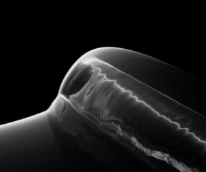
Figure 2. Measured crest profiles from a time shortly before jet formation to the time of jet impact for one realisation of the moderate breaker. Each surface profile, shown in blue, is obtained from one LIF image. Note, only the top portion of the plunging jet is visible in the surface profiles as discussed in § 2.3. Each successive profile is separated by a time interval of  $\Delta t = 0.0123$ s (every 8th frame in the LIF movie) and plotted ${{\rm d}\kern 0.05em y} = 25$ mm above the previous profile for clarity. The first profile, $n=1$, is located at the bottom of the plot. The locations of the crest point (the highest point on the wave crest) and jet tip are marked by green squares and red triangles, respectively, on each profile.
Wave crest profiles at  $t^f$ and $t^i$ from the 10 realisations of the strong breaker are presented in figure 3(a,b), respectively. The zero point of the $x$ coordinate in these plots is taken as the average horizontal position of the point of jet impact. In both plots, it can be seen that the 10 wave profiles are quite similar in shape, but the horizontal position of the profiles varies by approximately $3.5$ cm which is approximately 3 % of $\lambda _0$ and 50 % of $\overline {\langle r^i_x\rangle }$, the average horizontal distance from the jet impact point to the crest point, see figure 4. The crest height varies by approximately 1 mm, which is approximately 1.6 % of $\overline {\langle r^i_y\rangle }$, the vertical distance from the jet impact point to the crest point. It is thought that these variations are the result of slight variations in wave maker motion and in wave propagation through the tank water, which is probably contaminated by some residual motion from repeated runs. These residual motions include drift currents from the water surface skimming between runs and a small-amplitude seiche motion, which is typical of wave tank experiments with repeated runs, see § 2.5 for more details on the seiche. A table of the SD of the vertical and horizontal positions of the wave crest point at the moment of jet formation, denoted by $x^{f}_c$ and $y^{f}_c$, respectively, and the moment of jet impact, denoted by $x^{i}_{c}$ and $y^{i}_{c}$, respectively, are reported in table 5 of the Appendix.

Figure 3. Breaker profiles from 10 runs of the strong plunging breaker are shown in red at the time of (a) jet formation and (b) jet impact, respectively. The origin of the  $x\lambda ^{-1}_0$ axis in (a,b) is located at the mean of the 10 streamwise positions of jet impact. The profiles are otherwise not spatially or temporally aligned and therefore give an idea of the run-to-run repeatability of the strong breaker. Spatially and temporally aligned breaker profiles for 10 runs of the three breakers are shown in (c) for $t=t^f$ and (d) for $t=t^i$. The weak and strong breakers are indicated by the call-outs $W$ and $S$, respectively. In the axes legends of panels (c,d), $\tilde x\lambda _0^{-1} = (x-\Delta x^i_{b})\lambda _0^{-1}$ and $\tilde y\lambda _0^{-1} = (y-\Delta y^{i}_{c})\lambda _0^{-1}$. Details of the calculation of the alignment parameters $\Delta x^{i}_b$ and $\Delta y^{i}_c$ are discussed in the text.

Figure 4. Sketch showing the definition of various geometric and kinematic parameters of the wave profiles at the moment of jet formation, blue profile, and the moment of jet impact, red profile. Numerical values of the parameters for each of the three waves are given in table 2. The  $x$ and $y$ component of the wave crest speed are represented by $u_c$ and $v_c$, respectively, while $V^i_j$ and $\theta _{V^i_j}$ are the speed and angle of the jet tip velocity at impact. The slope of the front face of the jet around the point of jet impact is $\theta ^i_{j}$. The area under the plunging jet at impact, denoted by the pink background and labelled $Q^i$, is defined along with the major and minor axes of this area, $r^i_x$ and $r^i_y$.
Table 2. Geometric and kinematic wave parameters for the three breakers at the times of jet formation and jet impact. The  $\pm$ values with each average quantity indicate one SD as measured from the profiles of each of the 10 realisations of the breaker, while quantities without a $\pm$ value are measured directly from averaged breaker profiles. Most of the parameters are defined in figure 4. The time and $x$ and $y$ displacement of the jet tip from formation to impact are represented by $\Delta t^{f \text {-} i}$, $\Delta x^{f \text {-} i}_j$, $\Delta y^{f \text {-} i}_j$, respectively. The averaged $x$ and $y$ components of the accelerations of the wave crest and jet tip are represented by $a^{f \text {-} i}_{c,x}$, $a^{f \text {-} i}_{c,y}$, $a^{mj \text {-} i}_{j,x}$, $a^{mj \text {-} i}_{j,y}$ respectively. The maximum wave crest height relative to the still water level is given by $\langle y_{max} \rangle$.

In order to facilitate the creation of ensemble-averaged mean and SD profile histories for each of the three breakers during the ensuing turbulent phase of the breaking events, the profile sequences were aligned in time and space at the moment of jet impact. To perform this alignment, the time in each run is measured relative to the time of jet impact,  $\tilde t = t-t^i$, and offsets in $x$ and $y$ were determined as follows. The $x$ offsets were determined by sliding the individual profiles at $t^i$ from the 10 runs for each wave horizontally to minimise the difference between each profile and the average profile in the constant slope region (around the mean water level) on the back face of the wave. (This region of the profile was chosen for the alignment because it is nearly a straight line and of highly repeatable slope.) Thus, each profile of height is plotted vs $\tilde {x} = x-\Delta x^i_{\! b}$, where $\Delta x^i_{\! b}$ is the shift in $x$ required to align each profile with the average profile in the back face region. Recall also that $x=0$ is the average horizontal position of the jet tip at impact. The vertical coordinate of the aligned profiles is $\tilde y = y - \Delta y^i_{\! c}$ where the offsets, $\Delta y^i_{\! c}$, were determined by moving the profiles vertically, by at most a fraction of $1\ {\rm mm} =0.016\overline {\langle r^i_y\rangle }$, to align all profiles at their crest points with the average crest point height at the moment of jet impact. The variations of positions and times of the crest point and back face from each of the 10 realisations are listed in table 6 in the Appendix. The results of this alignment are shown in the plots of the jet formation and jet impact profiles in $(\tilde {x}\lambda _0^{-1},\tilde {y} \lambda _0^{-1})$ coordinates for the three breakers in figure 3(c,d), respectively. As can be seen from the profiles in figure 3(d), the maximum thickness of the band of aligned profiles for each of the three breakers is approximately $3.0\ {\rm mm} = 0.04\overline {\langle r^i_x\rangle }=0.0025\lambda _0$ and occurs in the jet tip region. It is believed that this small region of maximum misalignment is caused by run to run variations in the jet tip shape caused by transverse instabilities in the falling jet as observed in the LIF movies, see supplementary Movie 1, discussed in previous experimental studies including Perlin, He & Bernal (Reference Perlin, He and Bernal1996) and analysed theoretically in Longuet-Higgins (Reference Longuet-Higgins1995). Throughout the remaining regions of the profiles, the band thickness is no more than $1\ {\rm mm} = 0.014\overline {\langle r^i_x\rangle }=0.0009\lambda _0$. This alignment is critical to obtaining a reliable zero level of the SD of the non-breaking part of the breaker profile.
The profiles at  $t^f$ are plotted in $\tilde x$– $\tilde y$ coordinates in figure 3(c). The 10 crest profiles for each breaker are nearly as well aligned as those at $t^i$. The relative change in the locations of the wave crest in $\tilde x$– $\tilde y$ coordinates between jet formation and jet impact indicates that the horizontal distance travelled by the waves increases with increasing breaker intensity as does the increase in crest point height. Details of these results are given in the following subsection.
3.2. Breaker characterisation up to jet impact
In this subsection, the breaker profile histories are used to obtain quantitative measures of geometric and kinematic parameters describing the three breakers during the time between jet formation and jet impact. Values of many of these parameters at the moment of jet formation and/or jet impact are defined in figure 4 and reported in table 2. This set of parameters is similar to the set defined in figure 3 of Bonmarin (Reference Bonmarin1989) and includes the height from the jet impact point to the wave crest point, herein called  $r^i_y$, that was called $h$ and identified in Romero, Melville & Kless (Reference Romero, Melville and Kless2012), Derakhti & Kirby (Reference Derakhti and Kirby2014), Derakhti & Kirby (Reference Derakhti and Kirby2016), Deike, Popinet & Melville (Reference Deike, Popinet and Melville2015) and Deike, Melville & Popinet (Reference Deike, Melville and Popinet2016) as a key parameter characterising the post-impact breaking wave flows. Several of the measured quantities reported herein will be used later in this paper in correlations with features of the post-impact profiles and, in Reference Erinin, Liu, Wang, Liu and DuncanPart 2, with the measurements of droplet production.
Two quantities that describe the large-scale characteristics of the wave profile are the vertical distance  $H$ from the lowest point on the trough upstream of the breaking crest, called herein the trough point, to the crest point and the overall slope of the wave, $H/L$, where $L$ is the horizontal distance from the trough point to the crest point. Values of $\langle H \rangle$, $\langle L \rangle$ and $\langle H/L \rangle$ at $t=t^f$ and $t^i$ are given in table 2. The wave steepness at jet formation is calculated as $H^f/L^f$, see figure 4. From the values in the table, it can be seen that $H_f$ increases and $L^f$ decreases with increasing breaker strength, resulting in a 16 % increase in $H^f/L^f$ from the weakest to the strongest breaker. Comparisons of the measured values of $\langle H^f \rangle$ and $\langle H^f/L^f \rangle$ with the limiting form Stokes wavetrain and previously published experimental data is also useful. For a uniform wavetrain of frequency $f_0$ at the Stokes limit, the wave steepness is $H/\lambda = 0.1411$ (where $H$ is the crest-to-trough height and $\lambda$ is the wavelength) and $g\lambda /(2{\rm \pi} c^2) =0.8381$; see, for example, Longuet-Higgins (Reference Longuet-Higgins1984), Cokelet (Reference Cokelet1977), Schwartz (Reference Schwartz1974) and Zhong & Liao (Reference Zhong and Liao2018). Given that $c = f_0\lambda$ and taking $f_0=1.15$ Hz, we find $H_{Stokes} = 0.198$ m, $\lambda _{Stokes} = 1.193\lambda _0 = 1.408$ m and $c_{Stokes} = 1.193c_0=1.620$ m s $^{-1}$, where $c_0 = g/(2{\rm \pi} f_0) = 1.358$ m s $^{-1}$. In experimental data from breakers produced by various methods, see Ochi & Tsai (Reference Ochi and Tsai1983), Ramber & Griffin (Reference Ramberg and Griffin1987), Bonmarin (Reference Bonmarin1989) and Perlin et al. (Reference Perlin, He and Bernal1996), the measured values of $H$ are typically plotted against $gT^2$. In the present experiments, $gT_0^2= 7.42$ m and at this value the approximate range of $H$ in the above published experiments is from 8 cm to 17 cm. Thus, the values of $H$ in the present experiments (9.8–10.6 cm) are in the lower range of the values in the literature and all are below the value from the Stokes theory.
The ensemble-averaged horizontal and vertical positions of the wave crest point,  $\langle \tilde x_c \rangle \lambda _0^{-1}$ and $\langle \tilde y_c \rangle \lambda _0^{-1}$, respectively, for the three breakers are plotted vs $\tilde tf_0$, in figure 5(a,b), respectively. The $\langle \tilde x_c\rangle \lambda _0^{-1}$ vs $\tilde tf_0$ data for each of the three breakers form a single nearly straight line. The horizontal speed of the wave crest at jet formation, $\langle u^f_c \rangle$, was calculated by fitting a third-order polynomial to the ensemble-averaged dataset for each wave and evaluating the first derivative of the fitted curves at $t^f$. The values of $\langle u^f_c \rangle$, see table 2, are nearly the same for the three waves and the average of the three speeds is $1.52$ m s $^{-1}$. For reference, consider the phase speeds of linear and limiting form Stokes wave trains, $c_0 =1.358$ m s $^{-1}$ and $c_{Stokes} = 1.620$ m s $^{-1}$, respectively, as computed in the previous paragraph. The curves of the ensemble averaged crest point height, $\langle \tilde y_c\rangle \lambda _0$ vs $\tilde t f_0$, see figure 5(b), have an overall maximum at a time between $\langle t^f\rangle$ and $\langle t^i\rangle$. Near the time of jet formation, $y_c$ increases nearly linearly with time. A third-order polynomial was fitted to this ensemble-averaged data, see table 7, and the first derivative of the fits were evaluated at the moment of jet formation to yield the rate of rise of the crest, $\langle v^f_c \rangle$, with values of 0.105, 0.144 and 0.152 m s $^{-1}$ for the weak, moderate and strong breakers, respectively. From the moment of jet formation to the time when the crest reaches its maximum height, the vertical displacement of the crest point is approximately 8 mm for all three waves. After this maximum, the crest point drops about 2 mm before the moment of jet impact and continues to fall for a short time thereafter, eventually exhibiting irregular motion. The small SD found in this region of the plots indicates the high repeatability of this irregular motion of the crest point.

Figure 5. Ensemble-averaged dimensionless horizontal and vertical positions of the crest point,  $\langle \tilde x_c \rangle \lambda _0^{-1}$ and $\langle \tilde y_c\rangle \lambda _0^{-1}$, respectively, are plotted vs $\tilde t f_0$ in (a,b), respectively. Data are shown for the weak (green solid line), moderate (blue dashed line) and strong (red dotted line) breakers. The three coloured vertical lines indicate the average values of $\tilde t$ at the moment of jet formation for each of the three waves, whereas the vertical black line is the moment of jet impact ( $\tilde t =0$) for all three waves. The vertical half-width of the colour bands on each curve represents the SD of the data at each time instant. The coloured bands representing the SD for the data in (a) are too small to see in the plot. The slope of the dotted straight line in (a) is equal to the phase speed of a linear wave with frequency $f_0$, i.e. $c_p = 1.357$ m s $^{-1}$. The coloured squares mark the time of maximum wave crest height on each curve.
In the moments leading up to jet formation and impact, the wave becomes asymmetric as its forward face steepens. Just after the moment of jet formation, the jet tip begins to form and moves out ahead of the crest. The jet tip then, as is well known, simultaneously moves forward and falls to the water surface on the front face of the wave, entraining a pocket of air upon impact. The motion of the jet tip from jet formation to impact is presented in a plot of the ensemble average jet tip height,  $\langle \tilde y_j \rangle \lambda _0^{-1}$, vs $\tilde t f_0$ and a plot of the jet tip trajectory, $\langle \tilde y_j \rangle \lambda _0^{-1}$ vs $\langle \tilde x_j \rangle \lambda _0^{-1}$, in figure 6(a,b), respectively. Similar data for a single realisation of a plunging breaker can be found in Drazen et al. (Reference Drazen, Melville and Lenain2008). A cyan coloured ballistic curve is included in figure 6(a) for comparison with the jet tip data. Third-order polynomials were fitted to the ensemble-averaged $\langle \tilde x_j \rangle \lambda _0^{-1} - \tilde t f_0$ and $\langle \tilde y_j \rangle \lambda _0^{-1} - \tilde t f_0$ points from the time of maximum jet tip height to immediately before jet impact, see table 7. The jet tip velocity components at the moment of jet impact were obtained as the derivatives of these polynomials evaluated at $\tilde t = 0$ and the average speed $\langle V^i_j \rangle$ and angle $\langle \theta _{V^i_j} \rangle$ of this velocity for the three waves are given in table 2. The jet tip impact speed increases monotonically by 5.6 % (from 1.904 to 2.010 m s $^{-1}$) and the angle $\langle \theta _{V^i_j} \rangle$ increases from 21.9 $^\circ$ to 27.6 $^\circ$ as the breaker intensity increases from the weak to the strong breaker. It should be kept in mind that this is the angle made by the jet tip velocity vector; the angle of the front face of the jet as measured in a single LIF image, $\theta ^i_{\! j}$, at the time of jet impact is also included in the table. This angle is relatively independent of breaker intensity.

Figure 6. Ensemble-averaged dimensionless jet tip height,  $\langle \tilde y_j \rangle \lambda _0^{-1}$ is plotted vs $\tilde t f_0$, in panel (a) and vs the ensemble-averaged dimensionless jet tip horizontal position, $\langle \tilde x_j \rangle \lambda _0^{-1}$, in panel (b). See the caption of figure 5 for the key to the colours and line types of the curves and vertical lines in the plots. In panel (a), the solid cyan line is the free-fall ballistic trajectory and the coloured triangles indicate the location of the maximum jet tip height.
Brocchini & Peregrine (Reference Brocchini and Peregrine2001) used scaling arguments to predict the various types of disturbances of an air–water free surface produced by turbulent fluid motions. These surface disturbance types are identified in regions on a diagram with vertical axis,  $q$, defined as a ‘turbulent velocity scale’, and horizontal axis, $L$, defined as a length of the ‘most energetic turbulent scales’, see their figure 10. There are no direct measurements of these quantities in the present experiments, but if $q$ is taken as the speed of the jet tip at impact, $\langle V^i_j\rangle$, and $L$ as the vertical height from the jet tip to the crest point at impact, $\langle r^i_y\rangle$, then the three points for the present breakers, see table 2, when plotted in figure 10 of Brocchini & Peregrine (Reference Brocchini and Peregrine2001) are all in the zone at the top of their plot, which is labelled ‘ballistic’ and ‘splashing’.
The vertical acceleration of the jet tip was determined by taking the second derivative of the above-described third-order polynomials. It should be kept in mind that as second derivatives of measured trajectories, the accuracy of the accelerations is limited, approximately  $\pm$1.0 m s $^{-2}$. The average vertical component of the jet tip acceleration over the time span of the data, $\langle \bar {a}_{j,y} \rangle$, is found to be 7.43, 7.00 and 7.35 m s $^{-2}$ for the weak, moderate and strong breakers, respectively. These accelerations are about 18 % lower than the acceleration expected for a free falling object (see the curve from ballistic theory curve in figure 6a) and probably indicate the influence of surface tension and/or aerodynamic forces on the motion of the jet just before impact. In addition, the jet tip in this study is a temporally evolving geometrical point on the curved jet tip surface, not the position of a particle of mass. The average horizontal component of the acceleration of the jet tip over the same period of time, $\langle \bar {a}_{j,x} \rangle$, is found to be 1.030, 1.059 and 1.281 m s $^{-2}$ (in the direction of wave propagation, i.e. downstream) for the weak, moderate and strong breakers, respectively. The value of the horizontal acceleration in ballistic theory is, of course, equal to zero. Given the aforementioned accuracy figure, we cannot confidently identify any significant trend in the three vertical or horizontal acceleration values. The horizontal and vertical components of the distance travelled by the jet tip from formation to impact, $\Delta x_j$ and $\Delta y_j$, respectively, can be seen in figure 6(b) and are given in table 2. Both distances increase monotonically with increasing breaking intensity.
As can be seen from table 2, the variations in many of the above-described measured parameters are  $\lesssim$10% of their mean values over the three breakers. However, from qualitative observations of the LIF movies, one has the impression of a substantial increase in the scale and energy of the breaking region between the weak and the strong breaker, see Movies 2 and 3 given in the supplementary material. In addition, as will be described in Reference Erinin, Liu, Wang, Liu and DuncanPart 2, there is a substantial increase in the number of droplets as the breaker strength is increased. Exceptions to the geometrical quantities that vary by small percentages are the vertical component of the velocity of the crest at the moment of jet formation (50 % increase from the weak to the strong breaker), the vertical distance travelled by the jet tip (28 % increase) and the parameters $r^i_x$, $r^i_y$ and $Q^i$, that describe the geometry of the crest region at the moment of jet impact and increase by approximately, 42 %, 31 % and 86 %, respectively. The parameter $Q^i$ is the area under the upper surface of the plunging jet at impact, as shown by the coloured area labelled $Q^i$ in figure 4. (It should be emphasised that $Q^i$ is a geometrical parameter that is defined using only the profile of the upper surface of the jet and wave crest. The relationship between $Q^i$ and the cross-sectional area of the air tube entrapped under the jet at impact, $Q^i_{air}$, is likely to depend on the intensity of breaking as defined above and, through surface tension, the wavelength of the breaker. As noted in § 2.3, it is not possible to measure $Q^i_{air}$ with the present LIF technique. In lieu of measurements of $Q^i_{air}$, $Q^i$ will be used in Reference Erinin, Liu, Wang, Liu and DuncanPart 2 to correlate with the characteristics of the droplets generated by the breakers.) The increases in $r^i_x$ and $r^i_y$ are consistent with the increase in the upward vertical velocity of the crest, which is likely to indicate an increase in the vertical upward velocity of the jet tip as it is launched from the wave crest at $t=t^f$. This increase in vertical velocity might contribute to the increase in the horizontal distance travelled by the jet tip, resulting in impact with the wave face farther downstream where the water surface is lower. Plots of $\langle Q^i\rangle$ vs $\langle H^i/L^i\rangle$ at jet impact and $\langle v_c^f\rangle$ are given in figure 7(a,b), respectively. The plots indicate a nearly linear relationship (from only three data points) in both cases, however; the data in figure 7(a) conform to the linear fit more closely.

Figure 7. Estimated volume under the jet at the time of jet impact per unit length of crest,  $Q^i$, is plotted vs $\langle H^i/L^i\rangle$ and $\langle V^f_c\rangle$ in panels (a,b), respectively. In (a) the solid straight line is a linear fit of the form $Q= p_1\ (H^i/L^i)+p_2$ where $p_1 = 81\,250$ and $p_2 = -9786$, with $R^2 = 1$. In (b) the solid straight line is a linear fit of the form $Q= n_1\ \langle v^f_c \rangle +n_2$ where $n_1 = 37\,810$ and $n_2 = -1783$, with $R^2 = 0.96$.
3.3. Wave crest profile evolution after jet impact
The behaviour of the surface profile in the post-jet-impact time period is presented and discussed in this subsection. Detailed measurements of profiles over the breaking crest are examined first in § 3.3.1 with profile sequences presented in a reference frame moving with the wave crest. This is followed by an examination of the profile measurements covering the entire measurement plane in § 3.3.2, presented in laboratory-fixed coordinates. In all cases, ensemble averages and SDs are computed from profile sequences that are spatially and temporally aligned, see § 3.1.
3.3.1. Breaking region development and evolution after jet impact
After jet impact, significant run-to-run variations of the profiles are found in some spatial regions while in other regions the profiles are quite repeatable. The run-to-run variations are to be expected since at jet impact the flow begins transition to a temporally evolving and spatially non-uniform turbulent flow. An illustration of the run-to-run variation of the surface profiles after jet impact is given in figure 8(a) in which 10 profiles, one from each realisation of the strong breaker, all recorded  $\tilde t = 171\pm 12.3$ ms after jet impact, are shown along with the ensemble-averaged profile and a measure of SD, $n_{sd}$, see figure 8(b) for definition. Starting from the right and proceeding to the left (downstream in laboratory coordinates), the profiles are at first well aligned; the first local height maximum is the original crest of the breaker and the second maximum is both the current wave crest point (the highest point on the profile) and the top of the first splash zone. The local minimum, referred to below as an indentation, between these two maximums is the point where the upper surface of the plunging jet is now submerging under the splash zone. Farther downstream of the indentation, the run-to-run variation in surface height increases with the maximum variation occurring near the leading edge (called the toe) of the splash zone (also called the turbulent breaking region). In the region downstream of the toe, the profiles are nearly the same in each run. It should be noted that the entire region shown in the plot is downstream of the jet impact location, $\tilde x =0$.

Figure 8. (a) Breaker profiles in  $\tilde y\lambda _0^{-1}$– $\tilde x\lambda _0^{-1}$ coordinates from 10 realisations of the strong breaker (solid black lines) all measured $171 \pm 12.3$ ms after jet impact. The thick coloured line is the ensemble-averaged profile, where the colour contour along this line indicates the SD of the normal distance $n$,
$n$,  $n_{sd}=\sqrt {\langle [n-\langle n\rangle ]^2\rangle }/\lambda _{gc}$, where $n$ is defined in (b) as the distance between the average profile and the individual profiles measured at each point along the average profile in the direction of its local normal and $\lambda _{gc}=1.7$ cm, is the wavelength of the gravity-capillary wave with minimum phase speed. A second measure of profile variability, based on the profile local arc length, is also defined in (b) as the SD of the difference between the local arc length of the ensemble-averaged profile ( $s_m$) and the corresponding local arc length ( $s$) of the profile of a single realisation of the breaker non-dimensionalised by $s_m$, $s_{sd}=\sqrt {\langle [s/s_m-1]^2\rangle }$.
Details of the evolution of the ensemble-averaged profile and the SD profile histories of the crest region for the weak, moderate and strong breakers are more clearly seen in the sequences of profiles in figure 9(a–c), respectively. The plots are shown in a reference frame moving with the speed of the crest point at the moment of jet impact,  $\langle u^i_c\rangle$ (see table 2), and cover a streamwise width of $0.4\lambda _0$ and a time interval of $0.55f_0^{-1}$. Further details of the plots are given in the figure caption. In the moving reference frame of these plots, profile features that move faster (slower) than $\langle u^i_c\rangle$, move to the left (right) as time increases. The profiles in figure 9(a–c) are coloured locally according to the corresponding local value of $n_{sd}$. The horizontal and vertical positions of the indentations, the crest point and the toe of the splash, all extracted from the profiles in figure 9, are plotted vs time ( $\tilde t f_0$) in figure 10. Finally, for comparison, a profile history from a single realisation of the strong breaker is given in figure 9(d). Comparison of the ensemble-averaged (figure 9c) and single realisation (figure 9d) profile histories helps to demonstrate the repeatability of the process, particularly the space–time locations of the indentations and splashes.

Figure 9. Evolution of the ensemble-averaged crest profiles of the weak, moderate and strong breakers are presented in panels (a–c), respectively. Each line is the average profile at an instant in time,  $\tilde t_k$, after jet impact ( $k=0$) and the colour indicates the local value of the non-dimensional SD of the local normal distance, $n_{sd}$, see figure 8 its for definition. Each successive profile is plotted $\mathrm {d}\kern 0.05em y = 10$ mm above the previous profile and the temporal separation between profiles is $\tilde t_{k+1}- \tilde t_k = 0.0123$ s. The ninth breaker profile is marked by (i) and occurs at $\tilde{t} = 0.1107$ s; subsequent profiles marked by Roman numerals are 10 profiles apart. The profiles are shown in a reference frame moving with the speed of the crest point at the moment of jet impact, $\langle u^i_c\rangle$. The green squares mark the location of the highest point on each profile and the magenta upside down triangles are the local minimums of height in the indentations. A similar set of surface height profiles, but for only one realisation of the weakest breaker and plotted in the laboratory reference frame, was presented in Erinin et al. (Reference Erinin, Wang, Liu, Towle, Liu and Duncan2019). Panel (d) is a profile evolution plot for one realisation of the strong breaker.

Figure 10. Plots of the dimensionless coordinates of several features of the breaking wave crest are plotted vs  $\tilde t f_0$ in the laboratory reference frame. (a,b) The horizontal coordinates of the leading edge of the turbulent region (toe, $\tilde x_{toe} \lambda _0^{-1}$) and the local minima of the three indentations ( $\tilde x_k \lambda _0^{-1}$), respectively. (c,d) The horizontal ( $\tilde x_c \lambda ^{-1}$) and vertical ( $\tilde y_c \lambda ^{-1}$) coordinates of the crest point, respectively. The time range in each plot is from the moment of jet impact to $\approx$730 ms after jet impact, the same time interval as the profiles shown in figure 9. The vertical red dashed lines labelled (i) to (vi) in (c) are plotted at the times of the profiles in figure 9 with the same labels.
The repeatability of the early phase of the breaking process, including the jet impact and several cycles of splash generation and impact is demonstrated by the structure of each of the ensemble-averaged profile histories as well as the qualitative similarity of the profile histories of the three breaking waves in figure 9. Despite the fact that profiles are taken from the period in which the flow transitions from a laminar to a turbulent flow, many features of the profile histories are repeatable enough in space and time in each realisation to survive the ensemble averaging. The first repeatable feature is, of course, the average crest profile at the moment of jet impact, which is the first (lowest) profile. These are the same profiles of the crest region that are shown in figure 3(d). The  $n_{sd}$ magnitude along the first profile is essentially zero for each of the three breakers. Immediately after impact, an indentation forms between the plunging jet's upper surface and the splash generated by the first impact. This indentation quickly slows down and connects to the zone of very high $n_{sd}$ (between profiles (iii) and (iv) and centred near the horizontal position $-$0.2) that is associated with the bursting of bubbles entrapped under the plunging jet at the moment of impact, see Movie 4 included as supplementary material. The $n_{sd}$ level in this region increases monotonically with increasing breaking intensity, see § 3.3.2 for more details. The first indentation is also discussed in a number of studies including the experiments in Bonmarin (Reference Bonmarin1989) and the two-dimensional numerical computations in Iafrati (Reference Iafrati2009). In Bonmarin (Reference Bonmarin1989), the idea of air entrainment via this indention is discussed along with a few surface profiles, while in Iafrati (Reference Iafrati2009), analysis of the surface profile contours show that the indentation is deep and closes near the surface, entrapping a pocket of air. The LIF method in the present study only records the full depth of the indentation if the laser light rays are falling along the centreline of the cross-stream shape of the indentation and if the camera's line of sight is aligned with the indentation across the width of the tank. With a fixed camera, as in the present measurements, this alignment would only occur at one instant in time during a given breaking event. Since the cameras are stationary and not pointed across the tank width, the measured profiles indicate the location of the indentation, but not the deep centre of the cross section. In Reference Erinin, Liu, Wang, Liu and DuncanPart 2, it will be shown that a sheet of droplets is ejected at the instant in time when the indentation disappears in the profile sequence and that this disappearance is the result of the rapid rise of the bottom of the thin nearly vertical air crater at the indentation site.
The splash generated by the plunging jet impact forms a region of high  $n_{sd}$ but the motion of its leading edge, the toe, is highly repeatable, see the region of the splash zone between profiles (i) and (ii) and to the left of the first indentation in figure 9(a–c). Another two cycles of splash impact and generation are also visible with the second splash impact occurring between profiles (ii) and (iii) and the third between profiles (iii) and (iv). The impact–splash cycles are particularly prominent in the profiles from the two stronger breakers. After the initial jet impact, the leading edge of the turbulent breaking region accelerates downstream in all three profile histories and goes through cycles of accelerating and decelerating between profiles (ii) and (iv) as the splashes form and impact the wave face. The speed of the front splash region is close to the initial phase speed of the wave at several times, between surface profile (ii) and (v), but then decelerates by the time it reaches surface profile (vi). The horizontal position of the leading edge (toe) of the breaking region, $\langle \tilde x_\mathrm {toe}\rangle \lambda _0^{-1}$, is plotted vs $\tilde t f_0$ in figure 10(a). The toe position increases monotonically in time and, at any time, increases with breaker strength. There is evidence of some surging forward and backward in some of the curves, but the amplitude is small.
In a manner similar to the formation of the first indentation, with each splash impact an indentation forms between the plunging splash and the secondary splash that forms ahead of it. Each of these indentations at first moves at or near the speed  $\langle u_c^i\rangle$ and quickly slows down and falls behind the crest. The streamwise positions of these indentations, $\langle \tilde x_k\rangle$, were extracted from the ensemble-averaged profiles and are plotted in figure 10(b). The streamwise trajectory of the first indentation is nearly the same for the three breakers. The three trajectories of the second and third indentations are spread out in time and streamwise position, with the trajectories starting later in time and farther from the initial jet impact point as the breaker strength is increased.
The horizontal and vertical positions of the crest point (the highest point on each profile),  $\langle \tilde x_c\rangle \lambda _0^{-1}$ and $\langle \tilde y_c\rangle \lambda _0^{-1}$, respectively, are plotted vs $\tilde t f_0$ in figure 10(c,d), respectively. The crest point is also depicted as the green squares in the profile history plots in figure 9. The three curves of horizontal position in subplot (c) follow a similar trend with regions of nearly linear increase connected by jumps downstream at 0.201 $f_0^{-1}$, 0.437 $f_0^{-1}$, and 0.575 $f_0^{-1}$. Comparison with the profiles in figure 9(a–c), indicates that the jumps in $\langle \tilde x_c\rangle \lambda _0^{-1}$ occur as the crest point jumps across an indentation from the main crest to the first splash, from the first to the second splash, etc. The jumps occur at increasingly later times as the breaker intensity is increased. If one imagines a smooth curve going through the dataset for each wave, one can see that the curves for the three waves would be nearly the same, as are the raw data curves between each of the jumps. In addition, the local curve slope is higher for the overall curve than for the regions between jumps. The speed of the crest point in each of the linear segments, which are labelled by uppercase Roman numerals in figure 10(c), are listed in table 3. These speeds are substantially less than $\langle u^i_c\rangle$ and $c_0 =1.358$ m s $^{-1}$. The variable $\langle u^p/c\rangle$ in line one is the speed from a least-squares fit of a straight line to the data for each breaker over the entire range of the plot. These speeds are only a little less than $c_0$. As seen in figure 10(d), the height of the crest point, $\langle \tilde y_c\rangle \lambda _0^{-1}$, decreases dramatically after jet impact, approximately 0.05 $\lambda _0$ (a little more than 50 % of the maximum crest height, see last line of table 2) in a time interval $\Delta \tilde tf_0^{-1}=0.8$. It is thought that this decay is due partially to the conversion of wave energy to energy in the turbulence and due to the wave crest moving past the peak of the wave packet envelope. On top of this decaying curve is an oscillation with decaying amplitude; each local minimum occurs at the jump points in figure 10(c), where the crest point moves from one ripple to the next. The overall slopes and shapes of the curves are similar in the three breakers, but the decay occurs later in time as the breaker intensity is increased. This general behaviour of $x_c$ and $y_c$ is also seen in Bonmarin (Reference Bonmarin1989) (figures 23, 24, 26 and 28) where the positions of the breaking crest and the first and second splash-ups are plotted vs time for a single plunging breaking event.
Table 3. Post-impact horizontal speeds of the crest point and the toe of the three breakers. The speeds  $\langle u^P_c \rangle$ are from the slopes of straight lines fitted to the entire range of data in figure 10(c). The speeds $\langle u^I_c\rangle$ to $\langle u^{IV}_c\rangle$ are from the slopes of straight lines fitted to the nearly linear segments of the $\langle \tilde x_c\rangle$– $\tilde t f_0$ curves in figure 10(c). The horizontal speed of the splash front, $\langle u_{toe} \rangle$, is measured immediately following jet impact from $\tilde t = [0\ \mathrm {to}\ 0.14]$ using the data shown in figure 10(e).

3.3.2. Wave field evolution after jet impact
In this subsection, the surface profile measurements over the entire measurement region in time ( $-500\ {\rm ms} \leq \tilde t \leq 2500\ {\rm ms}$) and space ( $-0.3\ {\rm m} \leq \tilde x \le 1.0\ {\rm m}$) are presented and discussed. Data for the ensemble averaged surface height, the local surface normal distance SD ( $n_{sd}$), and the local arc length SD ( $s_{sd}$) on the $\tilde x \lambda _0^{-1}-\tilde t f_0$ plane are shown in figures 11–13, respectively. Each figure contains subplots for the weak, moderate, and strong breakers in (a–c), respectively. The profile and $n_{sd}$ data in figure 9 are from a diagonal band (tilted toward increasing $\tilde t f_0$ and $\tilde x \lambda _0^{-1}$) starting at the jet impact location in the contour plots in figures 11 and 12. The definitions of the local surface normal distance ( $n$) and the local arc length of the mean and instantaneous surface profiles ( $s_m$ and $s$), respectively, are given in figure 8(b). These two measures of SD were chosen to emphasise different features of the run-to-run variations of the profile shape, as is discussed in the following.

Figure 11. Contour maps of the non-dimensional mean surface height  $\langle \tilde y\rangle \lambda _{gc}^{-1}$ from 10 breaker realisations on the $\tilde x \lambda _0^{-1} \mathit {-} \, \tilde t f_0$ plane for the weak, moderate and strong breakers are given in panels (a), (b) and (c), respectively. The wavelength $\lambda _{cg} = 1.71$ cm is the wavelength of the gravity-capillary wave with minimum phase speed. The contour maps are shown in the laboratory reference frame for the full measurement region, $\approx$1300 mm in streamwise distance and $\approx$3000 ms in time and have a spatial and temporal resolution of $\Delta x = 0.165$ mm and $\Delta t = 12.3$ ms, respectively. The position and time of the maximum height of the wave crest point and the jet tip impact and are indicated by the green square and the red triangle, respectively. The call-outs A–E and the magenta downward triangles are discussed in the text. During the time approaching the maximum crest elevation, the back face of the breaking wave crest becomes partially obscured from the camera view and is not measured, as indicated by the white region just to the right of the green square in panels (a) and (b).

Figure 12. Contour maps of the non-dimensional SD of the local surface normal distance  $n_{sd}$ generated from 10 realisations on the $\tilde x \lambda _0^{-1} - \tilde t f_0$ plane for the (a) weak, (b) moderate and (c) strong plunging breakers. See figure 8(b) for definitions of $n_{sd}$. Plot details are given in the caption to figure 11.

Figure 13. Contour maps of the non-dimensional SD of the local arc length  $s_{sd}$ generated from 10 realisations on the $\tilde x \lambda _0^{-1} - \tilde t f_0$ plane for the (a) weak, (b) moderate and (c) strong plunging breakers. See figure 8(b) for definitions of $s_{sd}$. The dashed orange line in all three plots is the horizontal trajectory of a surface particle according to linear wave theory modified to include a large drift current, see the text for a discussion. The spatial resolution is $\Delta x = 2.740$ mm, other plot details are given in the caption to figure 11.
From the surface height contour maps shown in figure 11, the mean spatiotemporal evolution of the large-scale surface motion of the focusing wave packet can be analysed. The height contour maps for the three breakers are quite similar. Perhaps the most important wave feature in these plots is the trajectory of the main breaking wave crest, the yellow band indicated by A and travelling from right to left as time increases (vertically up in the subplots). The sharp yellow–green transition on the lower side of the breaker crest is near the toe of the turbulent breaking region. In the moments leading up to jet impact, the mean wave crest height reaches a maximum, indicated by the green square. The jet tip impact point is denoted by the red triangle at  $(\tilde x \lambda _0^{-1} , \tilde t f_0) = (0,0)$, after which the surface becomes irregular as the wave breaks, see discussion in § 3.3.1. In laboratory coordinates, the jet tip impact point for the weak breaker is located at $5.93$ m downstream from the back face of the wave maker, while the focusing distance parameter for the wave maker motion equation is $x_b = 6.17$ m, see (2.1). After the jet impact point, the breaking crest continues to decrease in amplitude while the amplitude of the crest following the breaker, indicated by D in the subplots, increases. This behaviour is consistent with the expected evolution of a deepwater wavetrain moving at its phase velocity through an amplitude envelope that moves in the same direction at the group velocity. A third crest of smaller height is barely visible in the upper right corner of the subplots. Shortly after jet impact, three indentations form sequentially on the main wave crest. The indentations are seen as faint dark orange lines in the otherwise yellow region at the breaker crest and are identified by the three sets of three magenta downward triangles drawn beginning at the heads of the three arrows at B in the three contour plots. These features were discussed in reference to the crest profile plots in figure 9 where the indentations can be seen more clearly in the sequences of profiles shown in crest-fixed coordinates. The downward magenta triangles for each indentation are the first, midrange and last downward magenta triangles of the corresponding indentation in figure 9(a–c).

Figure 14. Normalised arc length parameter  $\Delta s /\Delta x= (s-s_m)/\Delta x$ and normalised average normal displacement $\bar n/\Delta x$ both over a measurement interval $\Delta x$, see figure 8 for definitions, with the mean profile taken as a straight horizontal line ( $y=0$, length $s_m=\Delta x$) and an individual profile realisation taken as a sine wave, $y = a\sin kx$, where $k=2{\rm \pi} /\lambda$ and $\lambda$ is the wavelength. The measurement interval $\Delta x$ is from $x=0$ to $x=\lambda /2$. The slope of the $\bar n/\Delta x$ curve is $1/{\rm \pi} ^2=0.101$, while the slope of the $\Delta s/\Delta x$ curve is zero at $ak=0$ and asymptotes to a straight line with a slope of approximately 0.52 at $ak = 2.0$.
As mentioned previously, two measures of the local SD of the breaker profiles are presented herein: the normal distance SD,  $n_{sd}=\sqrt {\langle [n-\langle n\rangle ]^2\rangle }/\lambda _{gc}$, and the arc length SD, $s_{sd}= \sqrt {\langle [s/s_m -1]^2\rangle }$. Both quantities are dimensionless and are defined in figure 8(b). The normal distance SD was used in the discussion of the crest profile evolution in § 3.3.1. The normal distance was chosen rather than the vertical height as a measure of the difference between two water surface profiles because the height change exaggerates the miss match of the two curves when a small phase difference occurs between them at sharp profile features such as the bottom of the indentations discussed in § 3.3.1. The arc length SD is a measure of the relative shape of two profiles. If the individual and average profiles have the same shape and orientation over $\Delta x$, the difference in $s_{sd}$ is zero no matter the displacement ( $\bar {n}$) between the two curves. For the same curves, $n_{sd}$ would equal the displacement. If the shapes of the two curves are different over $\Delta x$ but the curves are on top of one another, the $n_{sd}$ may be small, while $s_{sd}$ can be large. In order to explore this difference numerically, a plot of these two quantities for an interval with an average profile consisting of a straight line (say $y=0$) and an individual profile consisting of a sine wave, $y = a\sin {kx}$, where $k = 2{\rm \pi} /\lambda$ and $\lambda$ is the wavelength, is given in figure 14. The arc length and $\bar n$ are computed over the interval $0\leq x \leq \lambda /2$. In this case, $\bar n$ is due to the shape of the profile within the interval $\Delta x$ and $\bar n = 2a/{\rm \pi}$. As can be seen from the figure, $\bar n$ varies linearly with $ak$ whereas the arc length at first increases more slowly than $\bar n$ but soon increases more rapidly. Thus, compared with $n_{sd}$, $s_{sd}$ is less sensitive to small slope disturbances and more sensitive to large slope disturbances. These differences in the behaviour of the two measures of SD create contour plots that emphasise different features of the surface roughness.
The contour plots of  $n_{sd}$ and $s_{sd}$ are given in figures 12 and 13, respectively. In these plots, the call-outs $A$ through $D$, the points of maximum crest height and jet impact, and the downward magenta triangles marking the locations of the indentations are identical to those in the corresponding subplots in figure 11. The most striking feature of all of the $n_{sd}$ and $s_{sd}$ contour plots is the sharp boundary between the low-SD-level region in the lower left (downstream, i.e. in the direction of wave travel) and the high-SD-level region of the front face of the wave crest. This boundary is slightly ahead, down and to the left, of the sharp blue–yellow transition in the panels in figure 11 and corresponds to the leading edge (toe) of the breaking region. The same boundary is visible in the $n_{sd}$ colour contours on each of the ensemble-averaged profiles shown in crest-fixed coordinates in figure 9. The lower left regions of the $n_{sd}$ and $s_{sd}$ contour plots correspond to the water surface upstream of the breaker and the low values of $n_{sd}$ and $s_{sd}$ in these regions are a testament to the repeatability of the ten realisations of the non-breaking sections of the wave profile in $\tilde x$– $\tilde t$ coordinates.
The  $n_{sd}$ contour plots in figure 12 show a number of interesting features. In the case of the weak breaker, figure 12(a), one can see three diffuse bright elongated regions along the locations of the three indentations in the height contour plots at positions $B$. The bright regions along the indentation locations become less distinct as the breaker intensity increases, see figure 12(b,c). A small region of high $n_{sd}$ contour levels is found at location $E$, in all three subplots. This location is in line with but well past the end of the first indentation. The $n_{sd}$ levels in these small regions, approximately 2.07, 3.20 and 3.43 mm in the weak, moderate and strong breakers, respectively, are the highest in each contour map. These dimensional values correspond to $0.025 H^i$, $0.036 H^i$ and $0.038 H^i$ and $0.039\langle r^i_y\rangle$, $0.049\langle r^i_y\rangle$ and $0.049\langle r^i_y\rangle$, for the weak, moderate and strong breakers, respectively. See figure 4 for the definitions and table 2 for values of $H^i$ and $\langle r^i_y\rangle$ for each breaker. Observations of the diffuse-light movies indicates that the patch of high-SD level corresponds to the location where the large air bubbles entrapped under the jet at impact escape from the back face of the wave well past the end of the trajectory of the first indentation, see Movie 4 given as supplementary material. The closing of the indentation crater, as discussed above, occurs well before the emergence of the bubbles entrapped under the plunging jet. This large bubble bursting region was also noted by other investigators in experiments, including Bonmarin (Reference Bonmarin1989) and Blenkinsopp & Chaplin (Reference Blenkinsopp and Chaplin2007), and in numerical calculations, including Wang et al. (Reference Wang, Yang and Stern2016) and Mostert et al. (Reference Mostert, Popinet and Deike2022).
In the remaining areas of the  $n_{sd}$ contour maps, the $n_{sd}$ level is lower than in the breaking crest region but exhibits some interesting well-organised features. The magnitude of $n_{sd}$ decreases in the trough ( $C$) between the breaking crest and following wave crest, increases again at the following wave crest ( $D$) to a lower level than on the breaker crest and falls off again after the second crest. The pattern of light blue small-scale features in the $n_{sd}$ contour plots in the area bounded by the breaking crest on the lower left edge and approximately by the location corresponding to that of the red dashed wavy line between $E$ and $D$ in the $s_{sd}$ contour plots in figure 13 is likely the manifestation of the breaker-generated turbulent flow. The slow downstream mean motion of the wavy boundary is consistent with the idea of turbulent vortical flow features moving with the fluid rather than the wave crest. The relatively high level of $n_{sd}$ at the following wave crest may be associated with an interaction between the flow field of the long wavelength carrier wave of the packet and the short waves generated by the turbulence (Phillips Reference Phillips1981; Longuet-Higgins Reference Longuet-Higgins1987; Miller, Shemdin & Longuet-Higgins Reference Miller, Shemdin and Longuet-Higgins1991), or the modification of the turbulence by the carrier wave flow field (Tucker & Reynolds Reference Tucker and Reynolds1968; Reynolds & Tucker Reference Reynolds and Tucker1975; Kevlahan & Hunt Reference Kevlahan and Hunt1996, Reference Kevlahan and Hunt1997; Hadzic, Hanjalic & Laurence Reference Hadzic, Hanjalic and Laurence2001). A larger-scale faint wavelike structure is visible in the upper right portion of the plot ( $F$) where as many as five waves measuring approximately 120 mm in wavelength can be seen. This wavy feature is clearly visible in the plot for the weak breaker. The source of these waves is unknown, but may be associated with the interaction of the waves with the tank walls.
Contour plots of  $s_{sd}$, are shown in figure 13. The bright regions of the $s_{sd}$ contour plots are located in the same general areas as those in the $n_{sd}$ contour plots and consist of many small bright spots and short streaks. Some of the highest average contour levels are at the leading edge of the breaking region, just to the left of the each of the three indentations and at the location of large bubble bursting that was also prominent in the $n_{sd}$ contour maps. The faint vertical lines at $\tilde x \lambda _0^{-1} \approx 0.18$ and 0.55 are due to the slight mismatching of the profiles at the boundaries of the three images from which each profile is extracted. The local arc length seems to be particularly sensitive to errors in profile continuity at these boundaries. The collections of bright spots and streaks form striations with swaying motion. The three brightest of these striations issue from the three indentations (the first (right most) is labelled $S1$), and striations with similar shape and lower intensity are constantly produced all along the breaking crest region. The striations persist for the entire time span of the plot, about 2.7 wave periods, and sway to the left on the back face of the two wave crests and to the right on the front face of the following wave crest. With the exception of the striation marked by the call-out $S_0$ and issuing from approximately the end of the rightmost arrow at call-out $B$, there is, on top of the swaying motions, a general motion downstream (to the left). A visual inspection of some of the LIF images indicates that many of the bright spots and streaks that make up these striations are signatures of short wavelength ripples and individual bubbles that are in the light sheet during one or more frames of one or more of the LIF movies. These signatures seem to be strong enough to survive the ensemble averaging. This supports the hypothesis that the striations are collections of signatures of surface features generated at the breaking crest and moving downstream with the water surface particle velocity. The faint rightmost striation ( $S_0$), which has only a small downstream drift, is thought to be in the region upstream of the breaking zone where the surface drift is caused primarily by nonlinear (non-breaking) wave motion. On the other hand, the surface drift affecting the surface features making up the other striations is thought to include a strong component due to the intense surface current created by the breaking process. The surface features downstream (toward the lower left in the plot) of the breaking zone may be generated by the impacts of droplets ejected with downstream trajectories from the breaking zone, as seen, for example, in Movie 4 given in the supplementary material.

Figure 15. Plots of  $(n_{sd})_{max}$ and $(s_{sd})_{ave}$ vs $Q^i$ are given in (a) and (b), respectively. The maximum value $(n_{sd})_{max}$ is the average value $n_{sd}$ in a region that is $11\Delta t=135.3$ ms by $301\delta x= 49.7$ mm centred at the peak value of $n_{sd}$ in the large bubble popping region on the back face of the breaker. The average value $(s_{sd})_{ave}$ is the average of $s_{sd}$ over a rectangular region defined by the corners $(\tilde x\lambda ^{-1}$, $\tilde t f_0) =(0, 0)$ and $(0.85,1.0)$. The solid line in each plot is a least-squares fit of a straight line to the three data points: $(n_{sd})_{max} = 4.33\times 10^{-5}Q^i + 0.0289$ in (a) and $(s_{sd})_{ave}= 5.79 \times 10^{-6}Q^i + 0.0411$ in (b).
To explore the wavy striations in the  $s_{sd}$ contour plots further, the trajectory given by
 \begin{equation} \tilde x = \tilde x_0 + a \cos(\omega (\tilde t-\tilde t_0))+U_d (\tilde t-\tilde t_0) \end{equation}
was fitted by eye to the first striation ( $S_1$) affected by a strong drift current in the three $s_{sd}$ contour plots. In this equation, the first term is a spatial phase shift, the second term mimics the orbital motion of the waves (with the carrier wave frequency $\omega$, amplitude $a$ and time shift $t_0$), and the third term mimics the motion due to a surface drift of constant speed $U_d$. The values of $x_0$, $t_0$, $a$,
$a$,  $T = 2{\rm \pi} /\omega$ and $U_d$ from the qualitative fitting are given in table 4 and its caption and the resulting trajectories are plotted as the dashed wavy red curves in the three panels of figure 13. The trajectories are qualitatively a good fit to the striation labelled $S1$ in each panel, and the striations further downstream (fitted curves not shown), for at least the first wave period after breaking. In later time, the striations seem to drift downstream at a rate slower than $U_d$. The computed values of $U_d$, 0.13, 0.18 and 0.21 m s $^{-1}$ for the weak, moderate and strong breakers, respectively, are substantial and approximately consistent with the fluid speeds in the wakes of breaking waves as reported in Duncan (Reference Duncan1981, Reference Duncan1983), Rapp & Melville (Reference Rapp and Melville1990) and Melville, Veron & White (Reference Melville, Veron and White2002). The coincidence of these trajectories and the patterns in the contour plots lend further support to the idea that the arc length SD is responding to small surface features, such as bubbles, that move along with the surface drift current. According to the fitting, this drift current increases with breaker strength.
Table 4. Parameters obtained by qualitative (visual) fitting of the drift velocity equation (3.1) to the arc length SD contour plots in figure 13. The wave period,  $T= 1.35$ s, and wave amplitude, $a=0.07$ m, used in the fitting function were the same for all three waves. The results are plotted as the wavy dashed red line in each figure.

Table 5. The SD in millimetres of the position of the wave crest point at the time of jet formation,  $x^{\, f}_{c}$ and $y^{\, f}_{c}$, and jet impact, $x^{i}_{c}$ and $y^{\, i}_{c}$, before and after breaker profile alignment.

Comparisons of the magnitudes of  $n_{sd}$ and $s_{sd}$ from one wave to another are also of interest. In the case of $n_{sd}$, the comparison is difficult because the contour maps consists of large fields of low-level signal with a few isolated areas of high-level signal. Average values over the entire measurement field or even over only the breaking wave crest have yielded very low levels that are not consistent with the qualitative appearance of the contour maps. Here, only a simple quantitative measure of $n_{sd}$ is chosen, a stable peak value obtained by averaging over a small region centred at the location with the maximum value, marked by $E$ in each panel. This area, measuring $0.156f_0^{-1}$ (135.3 ms) by $0.042\lambda _0$ (49.7 mm), essentially covers the yellow contour level region in the plot for the strong breaker, figure 13(c). The local maximum values obtained in this way are called $(n_{sd})_{max}$. Since the high $s_{sd}$ regions in the panels in figure 13 cover a large area, an average value is calculated over the large rectangle defined by the corners $(\tilde x\lambda ^{-1}$, $\tilde t f_0$) =(0, 0) and (0.85,1.0). This average value is given the symbol $(s_{sd})_{ave}$. Plots of $(n_{sd})_{max}$ and $(s_{sd})_{ave}$ vs $Q^i$ are given in figure 15(a,b), respectively, where the three data points in each plot appear to be form straight lines with positive slope, see figure caption for details. It should be noted that $(n_{sd})_{max}/\overline {\langle r_y^i\rangle }$ and $(s_{sd})_{ave}$ vary from 0.034 to 0.056 and from 0.0538 to 0.064, respectively, from the weak to the strong breaker.
4. Conclusions
An experimental study of the temporal evolution of the profiles of plunging breaking waves created with mechanically generated dispersively focused wave packets has been presented. The profiles have been measured with a cinematic LIF method with high temporal and spatial resolution (650 pps and 180  $\mathrm {\mu }$m pixel $^{-1}$, respectively) over a time period of 3.4 average wave periods and a streamwise position interval of 1.1 nominal breaker wave lengths. Three waves were studied and these waves were generated with wave maker motions with nearly the same shape (average frequency, 1.15 Hz) but different overall amplitudes. The three amplitudes were chosen to create breakers ranging from a weak plunging breaker, such that any reduction in amplitude created a spilling breaker, and a strong plunging breaker, such that any increase in amplitude created a breaker at a position at least one wavelength closer to the wave maker than the intended break point. These wave maker amplitudes differ by only approximately 8 % of their average. Each of the three breakers was generated and measured 10 times.
The water surface profiles extracted from the LIF images were first used to analyse the crest profiles during the period from the moment when the plunging jet starts to form to the moment when the plunging jet tip hits the front face of the wave. The profiles during this time period are exceedingly repeatable, save for a  $\pm$1.5 cm run-to-run variation in the streamwise position of the jet tip at impact. It was found that while many of the measured parameters, including the crest height, the horizontal speed of the highest point on the wave profile (called herein the crest point) and the jet tip velocity just before impact, differ by less than 10 % between the weakest and strongest breakers, several changed more substantially. The variables with more dramatic ranges include the vertical velocity of the crest point at the moment of jet formation, 45 %, the horizontal and vertical distances between the jet impact point and the crest point, approximately 35 %, and a measure of the area under the plunging jet at the moment of impact, 86 %.
Immediately after jet impact, the flow begins the transition to turbulent flow. To explore this phase of breaking, the 10 profile sequences of each wave were first aligned relative to the time and position of jet impact and then, at each instant in time, the ensemble-averaged profile and two measures of the distribution of SD along the average profiles were computed. The first measure of SD is the normal distance between each segment of the mean profile and the corresponding segments of each individual profile and the second is the difference between the arc length of corresponding segments of the mean and individual profiles. It is found that during this transition process there is a highly repeatable motion that appears in the ensemble-averaged profile series. The motion consists of the first jet impact and subsequent splash up, followed by two cycles of splash impact and secondary splash generation. At each impact site a prominent indentation appears. These structures at first move with the speed of the crest but quickly slow down as the wave crest moves through the self-generated turbulent flow field. From the LIF and diffuse light movies of the breaking events, it can be seen that the large air bubbles entrapped under the plunging jet at impact come to the surface and burst at a position and time just past the end of the first indentation, which at this point is on the back face of the breaking wave crest.
The  $\tilde x$– $\tilde t$ contour maps of the normal distance SD have a very low overall average while local regions of high SD are found at the leading edge of the turbulent breaking region, just upstream of the indentations, and the above-described location of the bursting of the large bubbles entrained under the plunging jet. The local average of peak value of $n_{sd}$ at the latter location increases from 3.4% to 5.6% of the vertical distance from the jet impact location to the wave crest from the weak to the strong breaker. The arc length is sensitive to sharply curved regions of the surface created by small waves and bubbles. The resulting $x$–
$x$– $t$ contour map reveals a wavy pattern induced by oscillatory fluid particle motion in the focused wavetrain accompanied by a strong downstream drift probably created by the drift motion of the highly nonlinear waves and by the surface current induced by breaking. The contour maps of the arc length SD are more evenly distributed and the average value over the breaker was computed. It is found that this average increases from 5.4% to 6.5% from the weak to the strong breaker.
Supplementary material and movies
Supplementary material and movies are available at https://doi.org/10.1017/jfm.2023.379.
Acknowledgements
The authors thank undergraduate students Benjamin Schaefer, Benjamin Cha and Nicholas Lawson for help with the image processing related to these experiments.
Funding
The support of the Division of Ocean Sciences of the National Science Foundation under grants OCE0751853, OCE1829943 and OCE1925060 is greatly acknowledged.
Declaration of interests
The authors report no conflict of interest.
Appendix. Profile alignment data and polynomial coefficients for crest point and jet tip trajectories
Here we provide tables of profile alignment data and polynomial coefficients for crest point and jet tip trajectories.
Table 5 shows the SD of the  $x$ and $y$ location of the wave crest point at the time of jet formation, which is discussed in § 3.1. The wave profile alignment in $x$,
$x$,  $y$ and $t$ for each of the 10 runs for the weak, moderate and strong plunging breakers is listed in table 6 and discussed in § 3.1. Finally, table 7 shows the coefficients and $R^2$ values from the fitting of the wave crest and jet tip trajectories, which are discussed in § 3.2.
Table 6. Variations in positions and times of the crest point (denoted by subscript  $c$) and the back face (denoted by subscript $b\!f$) at the times of jet formation (denoted by superscript $f$) and jet impact (denoted by superscript $i$) where, $\Delta x_{b}^{\, i} = x_{b}^{\, i} -\langle x_{b}^{\, i} \rangle$, $\Delta y_{c}^{\, i} = y_{c}^{\, i} -\langle y_{c}^{\, i} \rangle$, $\Delta t^i = t^i-\langle t^i \rangle$ and $\Delta t^f = t^f-\langle t^f \rangle$ for 10 realisations of each breaker. Times are given in milliseconds and distances are given in millimetres. The distances and times in this table can be non-dimensionalised by $\langle r^i_x\rangle$, $\langle r^i_y\rangle$, and $\langle \Delta t^{f \text {-} i}\rangle$ given in table 2.

Table 7. Coefficients from fitting third-order polynomials to the ensemble-averaged wave crest point trajectories,  $\langle \tilde x_c(t) \rangle$ and $\langle \tilde y_c(t) \rangle$, and the jet tip trajectories, $\langle \tilde x_j(t) \rangle$ and $\langle \tilde y_j(t) \rangle$, for the weak, moderate and strong breakers. The polynomials have the form $x(t) = at^3 + bt^2 + ct + d$ where $x$ is the position in metres, $t$ is time in seconds, $a$–
$a$– $d$ are the polynomial coefficients and $R^2$ is the coefficient of determination from the fitting procedure. The polynomials were fitted to data recorded in the time range $t^f -13.8\ {\rm ms}\leq t \leq t^i+13.8\ {\rm ms}$.


 Open access