


1. Introduction
The Lamb–Chaplygin dipole is a relative equilibrium solution of the two-dimensional (2-D) Euler equations in an unbounded domain  ${\mathbb {R}}^2$ that was independently obtained by Lamb (Reference Lamb1895, Reference Lamb1906) and Chaplygin (Reference Chaplygin1903); the history of this problem was surveyed by Meleshko & van Heijst (Reference Meleshko and van Heijst1994). The importance of the Lamb–Chaplygin dipole stems from the fact that this is a simple exact solution with a continuous vorticity distribution which represents a steadily translating vortex pair (Leweke, Le Dizès & Williamson Reference Leweke, Le Dizès and Williamson2016). Such objects are commonly used as models in geophysical fluid dynamics where they are referred to as ‘modons’ (Flierl Reference Flierl1987). Interestingly, despite the popularity of this model, the stability properties of the Lamb–Chaplygin dipole are still not well understood and the goal of the present investigation is to shed some new light on this question.
We consider an unbounded flow domain  $\varOmega := {\mathbb {R}}^2$ (‘ $:=$’ means ‘equal to by definition’). Flows of incompressible inviscid fluids are described by the 2-D Euler equation which can be written in the vorticity form as
 \begin{equation} \frac{\partial{\omega}}{\partial{t}} + (\boldsymbol{u} \boldsymbol{\cdot} \boldsymbol{\nabla}) \omega = 0 \quad \text{in}\ \varOmega, \end{equation}
where  $t \in (0,T]$ is the time with $T>0$ denoting the length of the interval considered, $\omega \, : \, (0,T] \times \varOmega \rightarrow {\mathbb {R}}$ is the vorticity component perpendicular to the plane of motion and $\boldsymbol {u} = [u_1, u_2]^{\rm T} \, : \, (0,T] \times \varOmega \rightarrow {\mathbb {R}}^2$ is a divergence-free velocity field (i.e. $\boldsymbol {\nabla } \boldsymbol {\cdot } \boldsymbol {u} = 0$). The space coordinate is denoted $\boldsymbol {x} = [x_1, x_2]^{\rm T}$. Introducing the streamfunction $\psi \, : \, (0,T] \times \varOmega \rightarrow {\mathbb {R}}$, the relation between the velocity and vorticity can be expressed as
 \begin{equation} \boldsymbol{u} = \boldsymbol{\nabla}^\perp \psi, \quad \text{where} \ \boldsymbol{\nabla}^\perp := \left[ \frac{\partial{}}{\partial{x_2}} ,- \frac{\partial{}}{\partial{x_1}} \right]^{\rm T} \ \text{and} \quad \Delta \psi ={-} \omega. \end{equation}
System (1.1)–(1.2) needs to be complemented with suitable initial and boundary conditions, and they are specified below.
In the frame of reference translating with the velocity  $-U \boldsymbol {e}_1$, where $U>0$ and $\boldsymbol {e}_i$, $i=1,2$, is the unit vector associated with the $i$th axis of the Cartesian coordinate system, equilibrium solutions of system (1.1)–(1.2) satisfy the boundary-value problem (Wu, Ma & Zhou Reference Wu, Ma and Zhou2006)
 $$\begin{gather} \Delta \psi = F(\psi), \quad \text{in} \ \varOmega, \end{gather}$$
 $$\begin{gather}\psi \rightarrow \psi_\infty := U x_2, \quad \text{for} \ |\boldsymbol{x}| \rightarrow \infty, \end{gather}$$
where the ‘vorticity function’  $F \, : \, {\mathbb {R}} \rightarrow {\mathbb {R}}$ need not be continuous. Clearly, the form of the equilibrium solution is determined by the properties of the function $F(\psi )$. Assuming without loss of generality that it has unit radius ( $a = 1$), the Lamb–Chaplygin dipole is obtained by taking
 \begin{equation} F(\psi) =\begin{cases} -b^2 (\psi - \eta), & \psi > \eta \\ 0, & \text{otherwise}, \end{cases} \end{equation}
where  $b \approx 3.8317059702075123156$ is the first root of the Bessel function of the first kind of order one, $J_1(b) = 0$, and $\eta \in (-\infty,\infty )$ is a parameter characterizing the asymmetry of the dipole (in the symmetric case $\eta = 0$). The solution of (1.3)–(1.4) then has the form of a circular vortex core of unit radius embedded in a potential flow. The vorticity and streamfunction are given by the following expressions stated in the cylindrical coordinate system $(r,\theta )$ (hereafter we adopt the convention that the subscript ‘0’ refers to an equilibrium solution).
• Inside the vortex core ( $0 < r \le 1$, $0 < \theta \le 2{\rm \pi}$):
(1.5a)$$\begin{gather} \omega_0(r,\theta) = \frac{2 U b}{J_0(b)} \left[J_1(br) \sin\theta - \frac{\eta b}{2 U} J_0(br)\right], \end{gather}$$(1.5b)$$\begin{gather}\psi_0(r,\theta) = \frac{2 U}{b J_0(b)} J_1(br) \sin\theta + \eta \left[ 1 - \frac{J_0(br)}{J_0(b)}\right]. \end{gather}$$
$0 < r \le 1$, $0 < \theta \le 2{\rm \pi}$):
(1.5a)$$\begin{gather} \omega_0(r,\theta) = \frac{2 U b}{J_0(b)} \left[J_1(br) \sin\theta - \frac{\eta b}{2 U} J_0(br)\right], \end{gather}$$(1.5b)$$\begin{gather}\psi_0(r,\theta) = \frac{2 U}{b J_0(b)} J_1(br) \sin\theta + \eta \left[ 1 - \frac{J_0(br)}{J_0(b)}\right]. \end{gather}$$• Outside the vortex core (
$r > 1$, $0 < \theta \le 2{\rm \pi}$):
(1.6a)$$\begin{gather} \omega_0(r,\theta) = 0, \end{gather}$$(1.6b)$$\begin{gather}\psi_0(r,\theta) = U \left(1 - \frac{1}{r}\right) \sin\theta. \end{gather}$$


The vortical core region is denoted  $A_0 := \{ \boldsymbol {x} \in {\mathbb {R}}^2 \, : \, \| \boldsymbol {x} \| \le 1 \}$ and $\partial A_0$ denotes its boundary. The streamline patterns inside $A_0$ in the symmetric ( $\eta = 0$) and asymmetric (
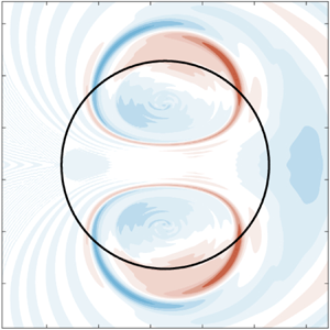
 $\eta > 0$) cases are shown in figures 1(a) and 1(b), respectively. Various properties of the Lamb–Chaplygin dipole are discussed by Meleshko & van Heijst (Reference Meleshko and van Heijst1994). In particular, it is shown that regardless of the value of $\eta$ the total circulation of the dipole vanishes, i.e. $\varGamma _0 := \int _{A_0} \omega _0 \, {\rm d}A = 0$. We note that in the limit $\eta \rightarrow \pm \infty$ the dipole approaches a state consisting of a monopolar vortex with a vortex sheet of opposite sign coinciding with the part of the boundary $\partial A_0$ above or below the flow centreline, respectively, for positive and negative $\eta$. Generalizations of the Lamb–Chaplygin dipole corresponding to differentiable vorticity functions $F(\psi )$ were obtained numerically by Albrecht, Elcrat & Miller (Reference Albrecht, Elcrat and Miller2011), whereas multipolar generalizations were considered by Viúdez (Reference Viúdez2019a,Reference Viúdezb).

Figure 1. Streamline pattern inside the vortex core  $A_0$ of (a) a symmetric ( $\eta = 0$) and (b) an asymmetric ( $\eta = 1/4$) Lamb–Chaplygin dipole. Outside the vortex core the flow is potential. The thick blue line represents the vortex boundary $\partial A_0$ whereas the red symbols mark the hyperbolic stagnation points $\boldsymbol {x}_a$ and $\boldsymbol {x}_b$.
Most investigations of the stability of the Lamb–Chaplygin dipole were carried out in the context of viscous flows governed by the Navier–Stokes system, beginning with the computations of dipole evolution performed by Nielsen & Rasmussen (Reference Nielsen and Rasmussen1997) and van Geffen & van Heijst (Reference van Geffen and van Heijst1998). While relations (1.5)–(1.6) do not represent an exact steady-state solution of the Navier–Stokes system, this approximate approach was justified by the assumption that viscous effects occur on time scales much longer than the time scales characterizing the growth of perturbations. A first such study of the stability of the dipole was conducted by Billant, Brancher & Chomaz (Reference Billant, Brancher and Chomaz1999) who considered perturbations with dependence on the axial wavenumber and found several unstable eigenmodes together with their growth rates by directly integrating the three-dimensional linearized Navier–Stokes equations in time. Additional unstable eigenmodes were found in the 2-D limit corresponding to small axial wavenumbers by Brion, Sipp & Jacquin (Reference Brion, Sipp and Jacquin2014). The transient growth due to the non-normality of the linearized Navier–Stokes operator was investigated in the related case of a vortex pair consisting of two Lamb–Oseen vortices by Donnadieu et al. (Reference Donnadieu, Ortiz, Chomaz and Billant2009) and Jugier et al. (Reference Jugier, Fontane, Joly and Brancher2020), whereas Sipp & Jacquin (Reference Sipp and Jacquin2003) studied Widnall-type instabilities of such vortex pairs. The effect of stratification on the evolution of a perturbed Lamb–Chaplygin dipole in three dimensions was considered by Waite & Smolarkiewicz (Reference Waite and Smolarkiewicz2008) and Bovard & Waite (Reference Bovard and Waite2016). The history of the studies concerning the stability of vortices in ideal fluids was recently surveyed by Gallay (Reference Gallay2019).
The only stability analysis of the Lamb–Chaplygin dipole in the inviscid setting we are aware of is due to Luzzatto-Fegiz & Williamson (Reference Luzzatto-Fegiz and Williamson2012) and Luzzatto-Fegiz (Reference Luzzatto-Fegiz2014) who employed methods based on imperfect velocity-impulse diagrams applied to an approximation of the dipole in terms of a piecewise-constant vorticity distribution and concluded that this configuration is stable. Finally, there is a recent mathematically rigorous result by Abe & Choi (Reference Abe and Choi2022) who established orbital stability of the Lamb–Chaplygin dipole (orbital stability implies that flows corresponding to ‘small’ perturbations of the dipole remain ‘close’ in a certain norm to the translating dipole; hence, this is a rather weak notion of stability).
As noted by several authors (Meleshko & van Heijst Reference Meleshko and van Heijst1994; Waite & Smolarkiewicz Reference Waite and Smolarkiewicz2008; Luzzatto-Fegiz & Williamson Reference Luzzatto-Fegiz and Williamson2012; Abe & Choi Reference Abe and Choi2022), the stability properties of the Lamb–Chaplygin dipole are still to be fully understood despite the fact that it was introduced more than a century ago. To the best of our knowledge, the present study is the first comprehensive investigation of the linear stability of the Lamb–Chaplygin dipole in the inviscid case, which is the only setting where it represents a true equilibrium solution of the governing equations. As a result, we find behaviour that was not observed in any of the earlier studies. It is demonstrated that the Lamb–Chaplygin dipole is in fact linearly unstable, but the nature of this instability is quite subtle and cannot be understood without referring to the infinite-dimensional nature of the linearized governing equations. More specifically, both the asymptotic and numerical solution of an eigenvalue problem for the 2-D linearized Euler operator suitably localized to the vortex core  $A_0$ confirm the existence of an essential spectrum with the corresponding approximate eigenfunctions in the form of short-wavelength oscillations localized near the vortex boundary $\partial A_0$. However, the time integration of the 2-D Euler system reveals the presence of a single exponentially growing eigenmode and since the corresponding eigenvalue is embedded in the essential spectrum of the operator, this unstable eigenmode is also found not to be a smooth function and exhibits short-wavelength oscillations. These findings are consistent with the general mathematical results known about the stability of equilibria in 2-D Euler flows (Shvydkoy & Latushkin Reference Shvydkoy and Latushkin2003; Shvydkoy & Friedlander Reference Shvydkoy and Friedlander2005) and have been verified by performing computations with different numerical resolutions and, in the case of the eigenvalue problem, with different arithmetic precisions.
The structure of the paper is as follows. In the next section we review some basic facts about the spectra of the 2-D linearized Euler equation and transform this system to a form in which its spectrum can be conveniently studied with an asymptotic method and numerically. A number of interesting properties of the resulting eigenvalue problem are also discussed, an approximate asymptotic solution of this eigenvalue problem is constructed in § 3, the numerical approaches used to solve the eigenvalue problem and the initial-value problem (1.1)–(1.2) are introduced in § 4, whereas the obtained computational results are presented in §§ 5 and 6. Discussion and final conclusions are deferred to § 7. Some more technical material is collected in three appendices.
2. Two-dimensional linearized Euler equations
The Euler system (1.1)–(1.2) formulated in the moving frame of reference and linearized around an equilibrium solution  $\{\psi _0,\omega _0\}$ has the following form, where $\psi ', \omega ' \, : \, (0,T] \times \varOmega \rightarrow {\mathbb {R}}$ are the perturbation variables (also defined in the moving frame of reference):
 \begin{gather}
\frac{\partial{\omega'}}{\partial{t}} ={-}
(\boldsymbol{\nabla}^\perp\psi_0 - U\boldsymbol{e}_1
)\boldsymbol{\cdot} \boldsymbol{\nabla}\omega' -
\boldsymbol{\nabla}^\perp\psi' \boldsymbol{\cdot}
\boldsymbol{\nabla}\omega_0 \nonumber\\ ={-}
(\boldsymbol{\nabla}^\perp\psi_0 - U\boldsymbol{e}_1
)\boldsymbol{\cdot} \boldsymbol{\nabla}\omega' +
\boldsymbol{\nabla}\omega_0 \boldsymbol{\cdot}
(\boldsymbol{\nabla}^\perp \varDelta^{{-}1})\omega'
\nonumber\\ =: {\mathcal{L}} \omega', \quad \text{in} \
\varOmega, \end{gather}
\begin{gather}
\frac{\partial{\omega'}}{\partial{t}} ={-}
(\boldsymbol{\nabla}^\perp\psi_0 - U\boldsymbol{e}_1
)\boldsymbol{\cdot} \boldsymbol{\nabla}\omega' -
\boldsymbol{\nabla}^\perp\psi' \boldsymbol{\cdot}
\boldsymbol{\nabla}\omega_0 \nonumber\\ ={-}
(\boldsymbol{\nabla}^\perp\psi_0 - U\boldsymbol{e}_1
)\boldsymbol{\cdot} \boldsymbol{\nabla}\omega' +
\boldsymbol{\nabla}\omega_0 \boldsymbol{\cdot}
(\boldsymbol{\nabla}^\perp \varDelta^{{-}1})\omega'
\nonumber\\ =: {\mathcal{L}} \omega', \quad \text{in} \
\varOmega, \end{gather}
 $$\begin{gather} \Delta\psi' ={-} \omega', \quad \text{in} \ \varOmega, \end{gather}$$
 $$\begin{gather}\psi' \rightarrow 0, \quad \text{for} \ |\boldsymbol{x}| \rightarrow \infty, \end{gather}$$
 $$\begin{gather}\omega'(0) = w', \quad \text{in} \ \varOmega, \end{gather}$$
in which  $\varDelta ^{-1}$ is the inverse Laplacian corresponding to the far-field boundary condition (2.1c) and $w'$ is an appropriate initial condition assumed to have zero circulation, i.e. $\int _{\varOmega } w'\, {\rm d}A = 0$. Unlike for problems in finite dimensions where, by virtue of the Hartman–Grobman theorem, instability of the linearized system implies the instability of the original nonlinear system, for infinite-dimensional problems this need not, in general, be the case. However, for 2-D Euler flows it was proved by Vishik & Friedlander (Reference Vishik and Friedlander2003) and Lin (Reference Lin2004) that the presence of an unstable eigenvalue in the spectrum of the linearized operator does indeed imply the instability of the original nonlinear problem.
Arnold's theory (Wu et al. Reference Wu, Ma and Zhou2006) predicts that equilibria satisfying system (1.3) are nonlinearly stable if  $F'(\psi ) \ge 0$, which, however, is not the case for the Lamb–Chaplygin dipole, since using (1.4) we have $F'(\psi _0) = -b^2 < 0$ for $\psi _0 \ge \eta$. Thus, Arnold's criterion is inapplicable in this case.
2.1. Spectra of linear operators
When studying spectra of linear operators, there is fundamental difference between the finite- and infinite-dimensional cases. To elucidate this difference and its consequences, we briefly consider an abstract evolution problem  ${\rm d}u/{\rm d}t = {\mathcal {A}} u$ on a Banach space ${\mathcal {X}}$ (in general, infinite-dimensional) with the state $u(t) \in {\mathcal {X}}$ and a linear operator ${\mathcal {A}} \, : \, {\mathcal {X}} \rightarrow {\mathcal {X}}$. Solution of this problem can be formally written as $u(t) = {\rm e}^{{\mathcal {A}} t} u_0$, where $u_0 \in {\mathcal {X}}$ is the initial condition and ${\rm e}^{{\mathcal {A}} t}$ the semigroup generated by ${\mathcal {A}}$ (Curtain & Zwart Reference Curtain and Zwart2013). While in finite dimensions linear operators can be represented as matrices which can only have point spectrum $\varPi _0({\mathcal {A}})$, in infinite dimensions the situation is more nuanced since the spectrum $\varLambda ({\mathcal {A}})$ of the linear operator ${\mathcal {A}}$ may in general consist of two parts, namely the approximate point spectrum $\varPi ({\mathcal {A}})$ (which is a set of numbers $\lambda \in {\mathbb {C}}$ such that $({\mathcal {A}} - \lambda )$ is not bounded from below) and the compression spectrum $\varXi ({\mathcal {A}})$ (which is a set of numbers $\lambda \in {\mathbb {C}}$ such that the closure of the range of $({\mathcal {A}} - \lambda )$ does not coincide with ${\mathcal {X}}$). We thus have $\varLambda ({\mathcal {A}}) = \varPi ({\mathcal {A}}) \cup \varXi ({\mathcal {A}})$ and the two types of spectra may overlap, i.e. $\varPi ({\mathcal {A}}) \cap \varXi ({\mathcal {A}}) \neq \emptyset$ (Halmos Reference Halmos1982). A number $\lambda \in {\mathbb {C}}$ belongs to the approximate point spectrum $\varPi ({\mathcal {A}})$ if and only if there exists a sequence of unit vectors $\{\,f_n\}$, referred to as approximate eigenvectors, such that $\|({\mathcal {A}} - \lambda ) f_n \|_{\mathcal {X}} \rightarrow 0$ as $n \rightarrow \infty$. If for some $\lambda \in \varPi ({\mathcal {A}})$ there exists a unit element $f$ such that ${\mathcal {A}} f = \lambda f$, then $\lambda$ and $f$ are an eigenvalue and an eigenvector of ${\mathcal {A}}$. The set of all eigenvalues $\lambda$ forms the point spectrum $\varPi _0({\mathcal {A}})$ which is contained in the approximate point spectrum, $\varPi _0({\mathcal {A}}) \subset \varPi ({\mathcal {A}})$. If $\lambda \in \varPi ({\mathcal {A}})$ does not belong to the point spectrum, then the sequence $\{\,f_n\}$ is weakly null convergent and consists of functions characterized by increasingly rapid oscillations as $n$ becomes large. The set of such numbers $\lambda \in {\mathbb {C}}$ is referred to as the essential spectrum $\varPi _{ess}({\mathcal {A}}) := \varPi ({\mathcal {A}}) \backslash \varPi _0({\mathcal {A}})$, a term reflecting the fact that this part of the spectrum is normally independent of boundary conditions in eigenvalue problems involving differential equations. It is, however, possible for ‘true’ eigenvalues to be embedded in the essential spectrum.
When studying the semigroup  ${\rm e}^{{\mathcal {A}} t}$ one is usually interested in understanding the relation between its growth abscissa $\gamma ({\mathcal {A}}) := \lim _{t \rightarrow \infty } t^{-1} \ln \| {\rm e}^{{\mathcal {A}} t} \|_{\mathcal {X}}$ and the spectrum $\varLambda ({\mathcal {A}})$ of ${\mathcal {A}}$. While in finite dimensions $\gamma ({\mathcal {A}})$ is determined by the eigenvalues of ${\mathcal {A}}$ with the largest real part, in infinite dimensions the situation is more nuanced since there are examples in which $\sup _{z \in \varLambda ({\mathcal {A}})} {\rm Re}(z) < \gamma ({\mathcal {A}})$, e.g. Zabczyk's problem (Zabczyk Reference Zabczyk1975) also discussed by Trefethen (Reference Trefethen1997); some problems in hydrodynamic stability where such behaviour was identified are analysed by Renardy (Reference Renardy1994).
In regard to the 2-D linearized Euler operator  ${\mathcal {L}}$, cf. (2.1a), it was shown by Shvydkoy & Latushkin (Reference Shvydkoy and Latushkin2003) that its essential spectrum is a vertical band in the complex plane symmetric with respect to the imaginary axis. Its width is proportional to the largest Lyapunov exponent $\lambda _{max}$ in the flow field and to the index $m \in {\mathbb {Z}}$ of the Sobolev space $H^m(\varOmega )$ in which the evolution problem is formulated (i.e. ${\mathcal {X}} = H^m(\varOmega )$ above). The norm in the Sobolev space $H^m(\varOmega )$ is defined as $\| u \|_{H^m} := [ \int _{\varOmega } \sum _{|\alpha | \le m} ({\partial ^{|\alpha |} u}/{\partial ^{\alpha _1} x_1 \partial ^{\alpha _2} x_2} )^2 \, {\rm d}A]^{1/2}$, where $\alpha _1,\alpha _2 \in {\mathbb {Z}}$ with $|\alpha | := \alpha _1+\alpha _2$ (Adams & Fournier Reference Adams and Fournier2005). More specifically, we have (Shvydkoy & Friedlander Reference Shvydkoy and Friedlander2005)
 \begin{equation} \varPi_{ess}({\mathcal{L}}) = \{ z \in {\mathbb{C}}, \ -|m| \lambda_{max} \le {\rm Re}(z) \le |m| \lambda_{max} \}. \end{equation}
 In 2-D flows Lyapunov exponents are determined by the properties of the velocity gradient  $\boldsymbol {\nabla }\boldsymbol {u}(\boldsymbol {x})$ at hyperbolic stagnation points $\boldsymbol {x}_0$. More precisely, $\lambda _{max}$ is given by the largest eigenvalue of $\boldsymbol {\nabla }\boldsymbol {u}(\boldsymbol {x})$ computed over all stagnation points. As regards the Lamb–Chaplygin dipole, it is evident from figure 1(a,b) that in both the symmetric and asymmetric cases it has two stagnation points $\boldsymbol {x}_a$ and $\boldsymbol {x}_b$ located at the fore and aft extremities of the vortex core. Inspection of the velocity field $\boldsymbol {\nabla }^\perp \psi _0$ defined in (1.5a) shows that the largest eigenvalues of $\boldsymbol {\nabla }\boldsymbol {u}(\boldsymbol {x})$ evaluated at these stagnation points, and hence the Lyapunov exponents, are $\lambda _{max} = 2$ regardless of the value of $\eta$.
While characterization of the essential spectrum of the 2-D linearized Euler operator  ${\mathcal {L}}$ is rather complete, the existence of a point spectrum remains in general an open problem. Results concerning the point spectrum are available in a few cases only, usually for shear flows where the problem can be reduced to one dimension (Chandrasekhar Reference Chandrasekhar1961; Drazin & Reid Reference Drazin and Reid1981) or the cellular cat's eyes flows (Friedlander, Vishik & Yudovich Reference Friedlander, Vishik and Yudovich2000). In these examples unstable eigenvalues are outside the essential spectrum (if one exists) and the corresponding eigenfunctions are well behaved. On the other hand, it was shown by Lin (Reference Lin2004) that when an unstable eigenvalue is embedded in the essential spectrum, then the corresponding eigenfunctions need not be smooth. One of the goals of the present study is to consider this issue for the Lamb–Chaplygin dipole.
2.2. Linearization around the Lamb–Chaplygin dipole
The linear system (2.1) is defined on the entire plane  ${\mathbb {R}}^2$; however, in the Lamb–Chaplygin dipole the vorticity $\omega _0$ is supported within the vortex core $A_0$ only, cf. (1.6b). This will allow us to simplify system (2.1) so that it will involve relations defined only within $A_0$, which will facilitate both the asymptotic analysis and numerical solution of the corresponding eigenvalue problem, cf. §§ 3 and 5. If the initial data $w'$ in (2.1d) are also supported in $A_0$, then the initial-value problem (2.1) can be regarded as a free-boundary problem describing the evolution of the boundary $\partial A(t)$ of the vortex core (we have $A(0) = A_0$ and $\partial A(t) = \partial A_0$). However, as explained below, the evolution of this boundary can be deduced from the evolution of the perturbation streamfunction $\psi '(t,\boldsymbol {x})$, hence need not be tracked independently. Thus, the present problem is different from, for example, the vortex-patch problem where the vorticity distribution is fixed (piecewise constant in space) and in the stability analysis the boundary is explicitly perturbed (Elcrat & Protas Reference Elcrat and Protas2013).
Denoting  $\psi _1' \, : \, (0,T] \times A_0 \rightarrow {\mathbb {R}}$ and $\psi _2' \, : \, (0,T] \times {\mathbb {R}}^2\backslash \bar {A}_0 \rightarrow {\mathbb {R}}$ the perturbation streamfunction in the vortex core and in its complement, system (2.1) can be recast as
 $$\begin{align} \frac{\partial{\omega'}}{\partial{t}} &={-} (\boldsymbol{\nabla}^\perp\psi_0 - U\boldsymbol{e}_1 )\boldsymbol{\cdot} \boldsymbol{\nabla}\omega' - \boldsymbol{\nabla}^\perp\psi_1' \boldsymbol{\cdot} \boldsymbol{\nabla}\omega_0, \quad \text{in} \ A_0, \end{align}$$
 $$\begin{align}\Delta\psi_1' &={-} \omega', \quad \text{in} \ A_0, \end{align}$$
 $$\begin{align}\Delta\psi_2' &= 0, \quad \text{in} \ {\mathbb{R}}^2\backslash \bar{A}_0, \end{align}$$
 $$\begin{align}\psi_1' &= \psi_2' = f', \quad \text{on} \ \partial A_0, \end{align}$$
 $$\begin{align}\frac{\partial{\psi_1'}}{\partial{n}} &= \frac{\partial{\psi_2'}}{\partial{n}} , \quad \text{on} \ \partial A_0, \end{align}$$
 $$\begin{align}\psi_2' &\rightarrow 0 , \quad \text{for} \ |\boldsymbol{x}| \rightarrow \infty, \end{align}$$
 $$\begin{align}\omega'(0) &= w', \quad \text{in} \ A_0, \end{align}$$
where  $\boldsymbol {n}$ is the unit vector normal to the boundary $\partial A_0$ pointing outside and conditions (2.3d)–(2.3e) represent the continuity of the normal and tangential perturbation velocity components across the boundary $\partial A_0$ with $f' \, : \, \partial A_0 \rightarrow {\mathbb {R}}$ denoting the unknown value of the perturbation streamfunction at that boundary.
The velocity normal to the vortex boundary  $\partial A(t)$ is $u_n := \boldsymbol {u} \boldsymbol {\cdot } \boldsymbol {n} = \partial \psi _1 / \partial s = \partial \psi _2 / \partial s$, where $s$ is the arc-length coordinate along $\partial A(t)$, cf. (2.3d). While this quantity identically vanishes in the equilibrium state (1.5)–(1.6), cf. (2.11), in general it will be non-zero resulting in a deformation of the boundary $\partial A(t)$. This deformation can be deduced from the solution of system (2.3) as follows. Given a point $\boldsymbol {z} \in \partial A(t)$, the deformation of the boundary is described by ${\rm d}\boldsymbol {z} / {\rm d}t = \boldsymbol {n} u_n|_{\partial A(t)}$. Integrating this expression with respect to time yields
 \begin{equation} \boldsymbol{z}(\tau) = \boldsymbol{z}(0) + \int_0^\tau \boldsymbol{n} u_n|_{\partial A_\tau} \, {\rm d}\tau' = \boldsymbol{z}(0) + \tau \boldsymbol{n} u_n|_{\partial A_0} + \mathcal{O}(\tau^2), \end{equation}
where  $\boldsymbol {z}(0) \in \partial A_0$ and $0 < \tau \ll 1$ is the time over which the deformation is considered. Thus, the normal deformation of the boundary can be defined as $\rho (\tau ) := \boldsymbol {n} \boldsymbol {\cdot }[ \boldsymbol {z}(\tau ) - \boldsymbol {z}(0)] \approx u_n|_{\partial A_0} \tau$. We also note that at the leading order the area of the vortex core $A(t)$ is preserved by the considered perturbations:
 \begin{equation} \oint_{\partial A_0} \rho(\tau) \, {\rm d}s = \tau \oint_{\partial A_0} \frac{\partial{\psi}}{\partial{s}} \, {\rm d}s = \tau \oint_{\partial A_0} \, {\rm d}\psi = 0 \Longrightarrow\ |A(t)| \approx |A_0|. \end{equation}
 We notice that in the exterior domain  ${\mathbb {R}}^2\backslash \bar {A}_0$ the problem is governed by Laplace's equation (2.3c) subject to boundary conditions (2.3d)–(2.3f). Therefore, this subproblem can be eliminated by introducing the corresponding Dirichlet-to-Neumann (D2N) map $M \, : \, \psi _2'|_{\partial A_0} \rightarrow \partial \psi _2'/\partial n|_{\partial A_0}$ which is constructed in an explicit form in Appendix A. Thus, (2.3c) with boundary conditions (2.3d)–(2.3f) can be replaced with a single relation $\partial \psi _1'/\partial n = M\psi _1'$ holding on $\partial A_0$ such that the resulting system is defined in the vortex core $A_0$ and on its boundary only. It should be emphasized that this reduction is exact as the construction of the D2N map does not involve any approximations. We therefore conclude that while the vortex boundary $\partial A(t)$ may deform in the course of the linear evolution, this deformation can be described based solely on quantities defined within $A_0$ and on $\partial A_0$ using relation (2.4). In particular, the transport of vorticity out of the vortex core $A_0$ into the potential flow is described by the last term on the right-hand side in (2.3a) evaluated on the boundary $\partial A_0$.
Noting that the base state satisfies the equation  $\Delta \psi _0 = - b^2 (\psi _0 - \eta )$ in $A_0$, cf. (1.3)–(1.4), and using the identity $(\boldsymbol {\nabla }^\perp \psi _1')\boldsymbol {\cdot } \boldsymbol {\nabla }\psi _0 = - (\boldsymbol {\nabla } \psi _1')\boldsymbol {\cdot } \boldsymbol {\nabla }^\perp \psi _0$, the vorticity equation (2.3a) can be transformed to the following simpler form:
 \begin{equation} \frac{\partial{\Delta \psi_1'}}{\partial{t}} ={-} (\boldsymbol{\nabla}^\perp \psi_0) \boldsymbol{\cdot} \boldsymbol{\nabla}(\Delta \psi_1' + b^2 \psi_1') \quad \text{in} \ A_0, \end{equation}
where we also used (2.3b) to eliminate  $\omega '$ in favour of $\psi _1'$. Supposing the existence of an eigenvalue $\lambda \in {\mathbb {C}}$ and an eigenfunction ${\tilde {\psi }} \, : \, A_0 \rightarrow {\mathbb {C}}$, we make the following ansatz for the perturbation streamfunction $\psi _1'(t,\boldsymbol {x}) = {\tilde {\psi }}(\boldsymbol {x}) \, {\rm e}^{\lambda t}$ which leads to the eigenvalue problem:
 $$\begin{align} \lambda {\tilde{\psi}} &= \varDelta_M^{{-}1} [ (\boldsymbol{\nabla}^\perp \psi_0) \boldsymbol{\cdot} \boldsymbol{\nabla}(\varDelta {\tilde{\psi}} + b^2 {\tilde{\psi}}) ] \quad \text{in} \ A_0, \end{align}$$
 $$\begin{align}\frac{\partial{\Delta {\tilde{\psi}}}}{\partial{r}} &= 0, \quad \text{at} \ r=0, \end{align}$$
where  $\varDelta _M^{-1}$ is the inverse Laplacian subject to the boundary condition $\partial {\tilde {\psi }} / \partial n - M{\tilde {\psi }} = 0$ imposed on $\partial A_0$ and the additional boundary condition (2.7b) ensures the perturbation vorticity is differentiable at the origin (such condition is necessary since the differential operator on the right-hand side in (2.7a) is of order three). Depending on whether or not the different differential operators appearing in it are inverted, eigenvalue problem (2.7) can be rewritten in a number of different, yet mathematically equivalent, forms. However, all these alternative formulations have the form of generalized eigenvalue problems and are therefore more difficult to handle in numerical computations. Thus, formulation (2.7) is preferred and we focus on it hereafter.
We note that the proposed formulation ensures that the eigenfunctions  ${\tilde {\psi }}$ have zero circulation, as required:
 \begin{align} \varGamma' &:= \int_{A_0} \omega' \, {\rm d}A ={-} \int_{A_0} \Delta \psi_1' \, {\rm d}A ={-} \oint_{\partial A_0} \frac{\partial{\psi_1'}}{\partial{n}} \, {\rm d}s\nonumber\\ & ={-} \oint_{\partial A_0} \frac{\partial{\psi_2'}}{\partial{n}} \, {\rm d}s ={-} \int_{{\mathbb{R}}^2 \backslash \bar{A}_0} \Delta \psi_2' \, {\rm d}A = 0, \end{align}
where we used the divergence theorem, (2.3b)–(2.3c) and the boundary conditions (2.3e)–(2.3f).
Since it will be needed for the numerical discretization described in § 5, we now rewrite the eigenvalue problem (2.7) explicitly in the polar coordinate system:
 $$\begin{align} \lambda {\tilde{\psi}} &= \varDelta_M^{{-}1}\left[ \left( u_0^r \frac{\partial{}}{\partial{r}} + \frac{u_0^\theta}{r} \frac{\partial{}}{\partial{\theta}} \right) (\varDelta + b^2 ) {\tilde{\psi}} \right] =: {\mathcal{H}} {\tilde{\psi}} \quad \text{for}\ 0 < r \le 1, \ 0 \le \theta \le 2{\rm \pi}, \end{align}$$
 $$\begin{align}\frac{\partial{\Delta {\tilde{\psi}}}}{\partial{r}} &= 0, \quad \text{at} \ r=0, \end{align}$$
where  $\varDelta = \partial ^2/\partial r^{2} + ({1}/{r})(\partial / \partial r) + ({1}/{r^2})(\partial ^2/\partial \theta ^2)$ and the velocity components obtained as $[ u_0^r, u_0^\theta ] := \boldsymbol {\nabla }^\perp \psi _0 = [ ({1}/{r})(\partial /\partial \theta ), -\partial /\partial r] \psi _0$ are
 $$\begin{align} u_0^r &= \frac{2U J_1(br)\cos\theta}{b J_0(b) r}, \end{align}$$
 $$\begin{align}u_0^\theta &={-} \frac{2U \left[ J_0(b r) - \dfrac{J_1(b r)}{b r} \right]\sin\theta + \eta b J_1(b r)}{J_0(b)}. \end{align}$$
They have the following behaviour on the boundary  $\partial A_0$:
 \begin{equation} u_0^r(1,\theta) = 0, \quad u_0^\theta(1,\theta) = 2U \sin\theta. \end{equation}
Since  $\|\psi \|_{L^2} \sim \| \Delta \psi \|_{H^{-2}} = \| \omega \|_{H^{-2}}$, where ‘ $\sim$’ means the norms on the left and on the right are equivalent (in the precise sense of norm equivalence), the essential spectrum (2.2) of the operator ${\mathcal {H}}$ will have $m = - 2$, so that $\varPi _{ess}({\mathcal {H}})$ is a vertical band in the complex plane with $|{\rm Re}(z)| \le 4$, $z \in {\mathbb {C}}$ (since $\lambda _{max} = 2$).
Operator  ${\mathcal {H}}$ (cf. (2.9a)) has a non-trivial null space $\operatorname {Ker}({\mathcal {H}})$. To see this, we consider the ‘outer’ subproblem
 $$\begin{align} {\mathcal{K}} \phi &:= \left( u_0^r \frac{\partial{}}{\partial{r}} + \frac{u_0^\theta}{r} \frac{\partial{}}{\partial{\theta}} \right) \phi = 0 \quad \text{for} \ 0 < r \le 1, \ 0 \le \theta \le 2{\rm \pi}, \end{align}$$
 $$\begin{align}\frac{\partial{\phi}}{\partial{r}} &= 0, \quad \text{at} \ r=0, \end{align}$$
whose solutions are  $\phi (r,\theta ) = \phi _C(r,\theta ) := B [J_1(br) \sin \theta ]^C$, $B \in {\mathbb {R}}$, $C = 2,3,\ldots$ (see Appendix B for derivation details). Then, the eigenfunctions ${\tilde {\psi }}_C$ spanning the null space of operator ${\mathcal {H}}$ are obtained as solutions of the family of ‘inner’ subproblems
 $$\begin{gather} \left( \frac{\partial^{2}}{\partial{r}^{2}} + \frac{1}{r} \frac{\partial{}}{\partial{r}} + \frac{1}{r^2} \frac{\partial^{2}}{\partial{\theta}^{2}} + b^2 \right) {\tilde{\psi}}_C = \phi_C \quad \text{for} \ 0 < r \le 1, \ 0 \le \theta \le 2{\rm \pi}, \end{gather}$$
 $$\begin{gather}\frac{\partial{{\tilde{\psi}}_C}}{\partial{r}} + M {\tilde{\psi}}_C = 0, \quad \text{at} \ r=0, \end{gather}$$
where  $C = 2,3,\ldots$. Some of these eigenfunctions are shown in figure 2(a–d), where distinct patterns are evident for even and odd values of $C$.
$C$.

Figure 2. Eigenfunctions  ${\tilde {\psi }}_C$, $C=$ (a) 2, (b) 3, (c) 4, (d) 5, corresponding to the zero eigenvalue of problem (2.9).
3. Asymptotic solution of eigenvalue problem (2.9)
A number of interesting insights about certain properties of solutions of eigenvalue problem (2.9) can be deduced by performing a simple asymptotic analysis of this problem in the short-wavelength limit. We focus here on the case of the symmetric dipole ( $\eta = 0$) and begin by introducing the ansatz
 \begin{equation} {\tilde{\psi}}(r,\theta) = \sum_{m=0}^{\infty} f_m(r) \cos(m\theta) + g_m(r)\sin(m\theta), \end{equation}
where  $f_m, g_m \, : \, [0,1] \rightarrow {\mathbb {C}}$, $m=1,2,\ldots$, are functions to be determined. Substituting this ansatz in (2.9a) with the Laplacian moved back to the left-hand side and applying well-known trigonometric identities leads after some algebra to the following system of coupled third-order ordinary differential equations for the functions $f_m(r)$, $m=1,2,\ldots$:
 \begin{gather}
\lambda {\mathcal{B}}_m
f_m = \frac{1}{2}P(r) \frac{{\rm d}}{{\rm d}r} (
{\mathcal{B}}_{m-1}f_{m-1} + b^2 f_{m-1} +
{\mathcal{B}}_{m+1}f_{m+1} + b^2 f_{m+1} ) \nonumber\\
\times \frac{1}{2}Q(r) \frac{m}{r} (
{\mathcal{B}}_{m-1}f_{m-1} + b^2 f_{m-1} -
{\mathcal{B}}_{m+1}f_{m+1} - b^2 f_{m+1} ), \quad r \in
(0,1), \end{gather}
\begin{gather}
\lambda {\mathcal{B}}_m
f_m = \frac{1}{2}P(r) \frac{{\rm d}}{{\rm d}r} (
{\mathcal{B}}_{m-1}f_{m-1} + b^2 f_{m-1} +
{\mathcal{B}}_{m+1}f_{m+1} + b^2 f_{m+1} ) \nonumber\\
\times \frac{1}{2}Q(r) \frac{m}{r} (
{\mathcal{B}}_{m-1}f_{m-1} + b^2 f_{m-1} -
{\mathcal{B}}_{m+1}f_{m+1} - b^2 f_{m+1} ), \quad r \in
(0,1), \end{gather}
 $$\begin{gather} f_m \quad \text{bounded}\quad \text{at} \ r = 0, \end{gather}$$
 $$\begin{gather}\frac{{\rm d}}{{\rm d}r} f_m ={-} m f_m \quad \text{at} \ r = 1, \end{gather}$$
 $$\begin{gather}\frac{{\rm d}}{{\rm d}r} {\mathcal{B}}_m f_m = 0 \quad \text{at} \ r = 0, \end{gather}$$
where the Bessel operator  ${\mathcal {B}}_m$ is defined via ${\mathcal {B}}_m f := ({{\rm d}^2}/{{\rm d}r^2}) f + ({1}/{r}) ({{\rm d}}/{{\rm d}r}) f - ({m^2}/{r}) f$, whereas the coefficient functions have the following form, cf. (2.10):
 $$\begin{gather} P(r) := \frac{2U J_1(br)}{b J_0(b) r}, \end{gather}$$
 $$\begin{gather}Q(r) :={-} \frac{2U \left[ J_0(b r) - \dfrac{J_1(b r)}{b r} \right]}{J_0(b)}. \end{gather}$$
The functions  $g_m(r)$, $m=1,2,\ldots$, satisfy a system identical to (3.2), which shows that the eigenfunctions ${\tilde {\psi }}(r,\theta )$ are either even or odd functions of $\theta$ (i.e. they are either symmetric or antisymmetric with respect to the flow centreline). Moreover, the fact that system (3.2) couples Fourier components corresponding to different $m$ implies that the eigenvectors ${\tilde {\psi }}(r,\theta )$ are not separable as functions of $r$ and $\theta$.
Motivated by our discussion in § 2.1 about the properties of approximate eigenfunctions of the 2-D linearized Euler operator, we construct approximate solutions of system (3.2) in the short-wavelength limit  $m \rightarrow \infty$. In this analysis we assume that $\lambda \in \varPi _{ess}({\mathcal {L}})$ is given and focus on the asymptotic structure of the corresponding approximate eigenfunctions. We thus consider the asymptotic expansions
 \begin{equation} \lambda = \lambda^0 + \frac{1}{m} \lambda^1 + {\mathcal{O}}\left(\frac{1}{m^2}\right), \quad f_m(r) = f_m^0(r) + \frac{1}{m} f_m^1(r) + {\mathcal{O}}\left(\frac{1}{m^2}\right), \end{equation}
where  $\lambda ^0, \lambda ^1 \in {\mathbb {C}}$ are treated as parameters and $f_m^0, f_m^1 \, : \, [0,1] \rightarrow {\mathbb {C}}$ are unknown functions. Plugging these expansions into system (3.2) and collecting terms proportional to the highest powers of $m$, we obtain
 \begin{align} &{\mathcal{O}}(m^3): \quad\quad\quad\quad
f_{m-1}^0 - f_{m+1}^0 = 0,
\end{align}
\begin{align} &{\mathcal{O}}(m^3): \quad\quad\quad\quad
f_{m-1}^0 - f_{m+1}^0 = 0,
\end{align} \begin{align}
&{\mathcal{O}}(m^2): \quad \frac{1}{2}
\frac{Q(r)}{r^3}(\,f_{m-1}^1 - f_{m+1}^1 ) =\frac{1}{2}
P(r) \frac{{\rm d}}{{\rm d}r}\left[ \frac{1}{r^2}
(\,f_{m-1}^0 + f_{m+1}^0) \right] \nonumber\\
& + \frac{Q(r)}{r^3}(\,f_{m-1}^0 + f_{m+1}^0 )
+ \frac{\lambda^0}{r^2} f_m^0.
\end{align}
\begin{align}
&{\mathcal{O}}(m^2): \quad \frac{1}{2}
\frac{Q(r)}{r^3}(\,f_{m-1}^1 - f_{m+1}^1 ) =\frac{1}{2}
P(r) \frac{{\rm d}}{{\rm d}r}\left[ \frac{1}{r^2}
(\,f_{m-1}^0 + f_{m+1}^0) \right] \nonumber\\
& + \frac{Q(r)}{r^3}(\,f_{m-1}^0 + f_{m+1}^0 )
+ \frac{\lambda^0}{r^2} f_m^0.
\end{align}
It follows immediately from (3.5a) that  $f_{m-1}^0 = f_{m+1}^0$. Since this analysis does not distinguish between even and odd values of $m$, we also deduce that $f_m^0 = f_{m-1}^0 = f_{m+1}^0$, such that relation (3.5b) takes the form
 \begin{equation} P(r) \frac{{\rm d}}{{\rm d}r}\left(\frac{1}{r^2} f_m^0 \right) - 2 \frac{Q(r)}{r^3} f_m^0 - \frac{\lambda^0}{r^2} f_m^0 = \frac{1}{2} \frac{Q(r)}{r^3}(\,f_{m-1}^1 - f_{m+1}^1 ), \quad r \in (0,1), \end{equation}
which is an inhomogeneous first-order equation defining the leading-order term  $f_m^0(r)$ in (3.4) in terms of $f_m^1(r)$. Without loss of generality the boundary condition (3.2b) can be replaced with $f_m^0(0) = 1$. The solution of (3.6) is then a sum of two parts: the solution of the homogeneous equation obtained by setting the right-hand side to zero and a particular integral corresponding to the actual right-hand side. Since at this level the expression $f_{m-1}^1 - f_{m+1}^1$ is undefined, we cannot find the particular integral. On the other hand, the solution of the homogeneous equation can be found directly noting that this equation is separable and integrating which gives
 \begin{equation} f_m^0(r) = \exp\left[ {\rm i} \int_0^r I_i(r') \, {\rm d}r' \right] \exp\left[ \int_0^r I_r(r') \, {\rm d}r' \right],\quad r \in [0,1], \end{equation}
where
 $$\begin{gather} I_r(r) := \frac{{\rm Re}(\lambda^0) b J_0(b) r^2 - 4 U b J_0(br) r + 8 U J_1 (br)}{2 U J_1(b r) r }, \end{gather}$$
 $$\begin{gather}I_i(r) := \frac{{\rm Im}(\lambda^0) b J_0(b) r}{2 U J_1(b r)}. \end{gather}$$
The limiting (as  $r \rightarrow 1$) behaviour of functions (3.8a)–(3.8b) exhibits an interesting dependence on $\lambda ^0$, namely:
 $$\begin{gather} \lim_{r \rightarrow 1} I_r(r) =\begin{cases} + \infty, & {\rm Re}(\lambda^0) < 4 \\ \phantom+ 0, & {\rm Re}(\lambda^0) = 4 \\ - \infty, & {\rm Re}(\lambda^0) > 4 , \end{cases} \end{gather}$$
 $$\begin{gather}\lim_{r \rightarrow 1} I_i(r) ={-} \operatorname{sign}[{\rm Im}(\lambda^0)] \infty. \end{gather}$$
In particular, the limiting value of  $I_r(r)$ as $r \rightarrow 1$ changes when ${\rm Re}(\lambda ^0) = 4$, which defines the right boundary of the essential spectrum in the present problem, cf. (2.2). Both $I_r(r)$ and $I_i(r)$ diverge as ${\mathcal {O}}(1/(1 - r))$ when $r \rightarrow 1$ which means that the integrals under the exponentials in (3.7), and hence the entire formula, are not defined at $r = 1$. While the factor involving $I_i(r)$ is responsible for the oscillation of the function $f_m^0(r)$, the factor depending on $I_r(r)$ determines its growth as $r \rightarrow 1$: we see that $|f_m^0(r)|$ becomes unbounded in this limit when ${\rm Re}(\lambda ^0) < 4$ and approaches zero otherwise. The real and imaginary parts of $f_m^0(r)$ obtained for different eigenvalues $\lambda ^0$ are shown in figure 3, where it is evident that both the unbounded growth and the oscillations of $f_m^0(r)$ are localized in the neighbourhood of the endpoint $r = 1$. Given the singular nature of the solutions obtained at the leading order, the correction term $f_m^1(r)$ is rather difficult to compute and we do not attempt this here. If $f_{m-1}^1 \neq f_{m+1}^1$, the solution of (3.6) will also include some extra terms in addition to (3.7)–(3.8) which would correspond to another possible family of approximate eigenfunctions. However, as is evident from the discussion below, the solutions given in (3.7)–(3.8) capture the relevant behaviour. Finally, in view of ansatz (3.1), the leading-order approximations to eigenfunctions are obtained multiplying the function $f_m^0(r)$ by $\cos (m \theta )$ or $\sin (m \theta )$ with $m \rightarrow \infty$ which introduces rapid oscillations in the azimuthal direction.

Figure 3. Radial dependence (a) of the eigenvectors  $f_m^0(r)$ associated with real eigenvalues $\lambda ^0 = 2$ (red solid line) and $\lambda ^0 = 6$ (blue dashed line) and (b) of the real part (red solid line) and the imaginary part (blue dashed line) of the eigenvector $f_m^0(r)$ associated with complex eigenvalue $\lambda ^0 = 3+10{\rm i}$. Panel (b) shows the neighbourhood of the endpoint $r=1$.
We thus conclude that when  ${\rm Re}(\lambda ^0) < 4$, the solutions of eigenvalue problem (2.9) constructed in the form (3.1) include functions dominated by short-wavelength oscillations whose asymptotic, as $m \rightarrow \infty$, structure involves oscillations in both the radial and azimuthal directions and are localized near the boundary $\partial A_0$. Since as a result their pointwise values on $\partial A_0$ are not well defined, these solutions should be regarded as ‘distributions’. We remark that the asymptotic solutions constructed above do not satisfy the boundary conditions (3.2c)–(3.2d), which is consistent with the fact that they represent approximate eigenfunctions associated with the essential spectrum $\varPi _{ess}({\mathcal {H}})$ of the 2-D linearized Euler operator. In order to find solutions of eigenvalue problem (2.9) which do satisfy all the boundary conditions, we have to solve this problem numerically which is done next.
4. Numerical approaches
In this section we first describe the numerical approximation of eigenvalue problem (2.9)–(2.10) and then the time integration of the 2-D Euler system (1.1)–(1.2) with the initial condition in the form of the Lamb–Chaplygin dipole perturbed with some approximate eigenfunctions obtained by solving eigenvalue problem (2.9)–(2.10). These computations offer insights about the instability of the dipole complementary to the results of the asymptotic analysis presented in § 3.
4.1. Discretization of eigenvalue problem (2.9)–(2.10)
Eigenvalue problem (2.9)–(2.10) is solved using the spectral collocation method proposed by Fornberg (Reference Fornberg1996), see also the discussion in Trefethen (Reference Trefethen2000), which is based on a tensor grid in  $(r,\theta )$. The discretization in $\theta$ involves trigonometric (Fourier) interpolation, whereas that in $r$ is based on Chebyshev interpolation where we take $r \in [-1,1]$ which allows us to avoid collocating (2.9a) at the origin when the number of grid points is even. Since then the mapping between $(r,\theta )$ and $(x_1,x_2)$ is 2-to-1, the solution must be constrained to satisfy the condition
 \begin{equation} {\tilde{\psi}}(r,\theta) = {\tilde{\psi}}({-}r,(\theta+{\rm \pi})(\text{mod} \ 2{\rm \pi})), \quad r \in [{-}1,1], \ \theta \in [0,2{\rm \pi}], \end{equation}
which is fairly straightforward to implement (Trefethen Reference Trefethen2000).
In contrast to (2.9a), the boundary condition (2.9b) does need to be evaluated at the origin which necessities modification of the differentiation matrix (since our Chebyshev grid does not include a grid point at the origin). The numbers of grid points discretizing the coordinates  $r \in [-1,1]$ and $\theta \in [0,2{\rm \pi} ]$ are linked and both given by $N$ which is an even integer. The resulting algebraic eigenvalue problem then has the form
 \begin{equation} \lambda \boldsymbol{\psi} = \boldsymbol{H} \boldsymbol{\psi}, \end{equation}
where  $\boldsymbol {\psi } \in {\mathbb {C}}^{N^2}$ is the vector of approximate nodal values of the eigenfunction and $\boldsymbol {H} \in {\mathbb {R}}^{N^2 \times N^2}$ the matrix discretizing the operator ${\mathcal {H}}$, cf. (2.9a), obtained as described above. Problem (4.2) is implemented in MATLAB and solved using the function eig. The discretization of all operators in ${\mathcal {H}}$, cf. (2.9), was carefully verified by applying them to analytic expressions and then comparing the results against exact expressions. Expected rates of convergence were observed as the resolution $N$ was increased.
Since the operator  ${\mathcal {H}}$ and hence also the matrix $\boldsymbol {H}$ are non-normal and singular, the numerical conditioning of problem (4.2) may be poor, especially when the resolution $N$ is refined. In an attempt to mitigate this potential difficulty, we eliminated a part of the null space of $\boldsymbol {H}$ by performing projections on a certain number $N_C$ of eigenfunctions associated with the eigenvalue $\lambda = 0$ (they are obtained by solving problem (2.13) with different source terms $\phi _C$, $C = 2,3,\ldots,N_C+1$; cf. (B4)). However, solutions of problem (4.2) obtained in this way were essentially unchanged as compared with the original version. Moreover, in addition to examining the behaviour of the results when the grid is refined (by increasing the resolution $N$ as discussed in § 5), we have also checked the effect of arithmetic precision using the toolbox Advanpix (Reference Advanpix2017). Increasing the arithmetic precision up to ${\mathcal {O}}(10^2)$ significant digits was also not found to have a noticeable effect on the results obtained with small and medium resolutions $N \le 100$ (at higher resolutions the cost of such computations becomes prohibitive). These observations allow us to conclude that the results presented in § 5 are not affected by round-off errors.
In the light of the discussion in §§ 2.1 and 2.2, we know that the spectrum of the operator  ${\mathcal {H}}$ includes essential spectrum in the form of a vertical band in the complex plane $|{\rm Re}(z)| \le 4$, $z \in {\mathbb {C}}$. Available literature on the topic of numerical approximation of infinite-dimensional non-self-adjoint eigenvalue problems, especially ones featuring essential spectrum, is very scarce. However, since the discretized problem (4.2) is finite-dimensional and therefore can only have a point spectrum, it is expected that at least some of the eigenvalues of the discrete problem will be approximations of the approximate eigenvalues in the essential spectrum $\varPi _{ess}({\mathcal {H}})$, whereas the corresponding eigenvectors will approximate the approximate eigenfunctions (we note that the term ‘approximate’ is used here with two distinct meanings: its first appearance refers to the numerical approximation and the second to the fact that these functions are defined as only ‘close’ to being true eigenfunctions, cf. § 2.1). As suggested by the asymptotic analysis presented in § 3, these approximate eigenfunctions are expected to be dominated by short-wavelength oscillations which cannot be properly resolved using any finite resolution $N$. Thus, since these eigenfunctions are not smooth, we do not expect our numerical approach to yield an exponential convergence of the approximation error. To better understand the properties of these eigenfunctions, we also solve a regularized version of problem (2.9) in which ${\tilde {\psi }}$ is replaced with ${\tilde {\psi }}_{\delta } := {\mathcal {R}}_{\delta }^{-1} {\tilde {\psi }}$, where ${\mathcal {R}}_{\delta } := (\operatorname {Id} - \delta ^2 \varDelta )$, $\delta > 0$ is a regularization parameter and the inverse of ${\mathcal {R}}_\delta$ is defined with the homogeneous Neumann boundary conditions. The regularized version of the discrete problem (4.2) then takes the form
 \begin{equation} \lambda_{\delta} \boldsymbol{\psi} = \boldsymbol{R}_{\delta} \boldsymbol{H} \boldsymbol{R}_{\delta}^{{-}1} \boldsymbol{\psi} =: \boldsymbol{H}_{\delta} \boldsymbol{\psi}, \end{equation}
where the subscript  $\delta$ denotes regularized quantities and $\boldsymbol {R}_{\delta }$ is the discretization of the regularizing operator ${\mathcal {R}}_{\delta }$. Since the operator ${\mathcal {R}}_{\delta }^{-1}$ can be interpreted as a low-pass filter with the cut-off length given by $\delta$, the effect of this regularization is to smoothen the eigenvectors by filtering out components with wavelengths less than $\delta$. Clearly, in the limit when $\delta \rightarrow 0$ the original problem (4.2) is recovered. An analogous strategy was successfully employed by Protas & Elcrat (Reference Protas and Elcrat2016) in their study of the stability of Hill's vortex where the eigenfunctions also turned out to be singular distributions.
4.2. Solution of the time-dependent problem (1.1)–(1.2)
The 2-D Euler system (1.1)–(1.2) is transformed to the frame of reference moving with velocity  $-U \boldsymbol {e}_1$ and rewritten in terms of the ‘perturbation’ vorticity ${\bar {\omega }}(t,\boldsymbol {x}) := \omega (t,\boldsymbol {x}) - \omega _0(\boldsymbol {x})$ and the corresponding perturbation streamfunction ${\bar {\psi }}(t,\boldsymbol {x})$, such that it takes the following form, cf. (2.1):
 $$\begin{align} &\frac{\partial{{\bar{\omega}}}}{\partial{t}} + (\boldsymbol{\nabla}^\perp {\bar{\psi}} - U \boldsymbol{e}_1 ) \boldsymbol{\cdot} \boldsymbol{\nabla}\omega_0 + (\boldsymbol{\nabla}^\perp \psi_0 + \boldsymbol{\nabla}^\perp {\bar{\psi}} - U \boldsymbol{e}_1 ) \boldsymbol{\cdot} \boldsymbol{\nabla}{\bar{\omega}}= 0 \quad \text{in} \ \varOmega, \end{align}$$
 $$\begin{align}- &\Delta {\bar{\psi}} = {\bar{\omega}} \quad \text{in} \ \varOmega, \end{align}$$
 $$\begin{align}& {\bar{\psi}} \rightarrow 0 \quad \text{for} \ |\boldsymbol{x}| \rightarrow \infty. \end{align}$$
To facilitate solution of this system with a Fourier pseudospectral method (Canuto et al. Reference Canuto, Hussaini, Quarteroni and Zang1988), we approximate the unbounded domain with a 2-D periodic box  $\varOmega \approx {\mathbb {T}}^2 := [-L/2,L/2]^2$, where $L > 1$ is its size. While this is an approximation only, it is known to become more accurate as the size $L$ of the domain increases relative to the radius of the dipole which remains fixed at one (Boyd Reference Boyd2001). We note that this is a standard approach and has been successfully used in earlier studies of related problems (Nielsen & Rasmussen Reference Nielsen and Rasmussen1997; van Geffen & van Heijst Reference van Geffen and van Heijst1998; Billant et al. Reference Billant, Brancher and Chomaz1999; Donnadieu et al. Reference Donnadieu, Ortiz, Chomaz and Billant2009; Brion et al. Reference Brion, Sipp and Jacquin2014; Jugier et al. Reference Jugier, Fontane, Joly and Brancher2020). Since the instability has the form of short-wavelength oscillations localized on the dipole boundary $A_0$, interaction of the perturbed dipole with its periodic images does not have a significant effect.
The perturbation vorticity is then approximated in terms of a truncated Fourier series:
 \begin{equation} {\bar{\omega}}(t,\boldsymbol{x}) \approx \sum_{\boldsymbol{k} \in V_M} \hat{{\bar{\omega}}}_{\boldsymbol{k}}(t) \, {\rm e}^{{\rm i} \boldsymbol{k} \ \cdot \ \boldsymbol{x}}, \end{equation}
in which  $\hat {{\bar {\omega }}}_{\boldsymbol {k}}(t) \in {\mathbb {C}}$ are the Fourier coefficients such that $\hat {{\bar {\omega }}}_{\boldsymbol {k}}(t) = \hat {{\bar {\omega }}}^*_{-\boldsymbol {k}}(t)$ and $V_M := \{ \boldsymbol {k} = [k_1,k_2] \in {\mathbb {Z}}^2 \, : \, -M/2 \le k_1, k_2 \le M/2 \}$, where $M$ is the number of grid points in each direction in ${\mathbb {T}}^2$. Substitution of expansion (4.5) into (4.4a) yields a system of coupled ordinary differential equations describing the evolution of the expansion coefficients $\hat {{\bar {\omega }}}_{\boldsymbol {k}}(t)$, $\boldsymbol {k} \in V_M$, which is integrated in time using the RK4 method. Product terms in the discretized equations are evaluated in physical space with the exponential filter proposed by Hou & Li (Reference Hou and Li2007) used in lieu of dealiasing. We use a massively parallel implementation based on MPI with Fourier transforms computed using the FFTW library (Frigo & Johnson Reference Frigo and Johnson2003). Convergence of the results with refinement of the resolution $M$ and of the time step $\Delta t$ as well as with the increase of the size $L$ of the computational domain was carefully checked. In the results reported in § 6 we use $L = 2{\rm \pi}$.
5. Solution of the eigenvalue problem
In this section we describe solutions of the discrete eigenvalue problem (4.2) and its regularized version (4.3). We mainly focus on the symmetric dipole with  $\eta = 0$; cf. figure 1a. In order to study dependence of the solutions on the numerical resolution, problems (4.2)–(4.3) were solved with $N$ ranging from 20 to 260, where the largest resolution was limited by the amount of RAM available on a single node of the computer cluster to which we had access. The discrete spectra of problem (4.2) obtained with $N = 40$, 80, 160, 260 are shown in figure 4(a–d). We see that for all resolutions $N$ the spectrum consists of purely imaginary eigenvalues densely packed on the vertical axis and a ‘cloud’ of complex eigenvalues clustered around the origin (for each $N$ is there is also a pair of purely real spurious eigenvalues increasing as $|\lambda | = {\mathcal {O}}(N)$ when the resolution is refined; they are not shown in figure 4(a–d). We see that as $N$ increases the cloud formed by the complex eigenvalues remains restricted to the band $-2 \lessapprox {\rm Re}(\lambda ) \lessapprox 2$, but expands in the vertical (imaginary) direction. The spectrum is symmetric with respect to the imaginary axis as is expected for a Hamiltonian system. The eigenvalues fill the inner part of the band ever more densely as $N$ increases and in order to quantify this effect, in figure 5(a–d) we show the eigenvalue density defined as the number of eigenvalues in a small rectangular region of the complex plane, i.e.
 \begin{align} \mu(z) := \frac{\text{number of eigenvalues } \lambda \in \{ \zeta \in {\mathbb{C}} \, : \, |{\rm Re}(\zeta -z)| \le \Delta\lambda_r, \ |{\rm Im}(\zeta -z)| \le \Delta\lambda_i \}} {4 \Delta\lambda_r \Delta\lambda_i}, \end{align}
where  $\Delta \lambda _r, \Delta \lambda _i \in {\mathbb {R}}$ are half-sizes of a cell used to count the eigenvalues with $\Delta \lambda _i \approx 500 \Delta \lambda _r$ reflecting the fact that the plots are stretched in the vertical direction. We see that as the resolution $N$ is refined the eigenvalue density $\mu (z)$ increases near the origin.

Figure 4. Eigenvalues obtained by solving the discrete eigenvalue problem (4.2) with different indicated resolutions  $N$: (a) $N=40$, (b) $N = 80$, (c) $N = 160$, (d) $N= 260$. The eigenvalues $\pm \lambda _0$ and $\pm \lambda _0^*$ which converge to well-defined limits as the resolution $N$ is refined, cf. Table 1, are marked in red. The eigenvalue $\lambda _0$ is associated with the only linearly unstable mode, cf. § 6.


Table 1. Eigenvalue  $\lambda _0$ associated with the linearly growing mode, cf. § 6, obtained by solving the discrete eigenvalue problem (4.2) with different resolutions $N$.
$N$.

As discussed in § 2.1, a key question concerning the linear stability of 2-D Euler flows is the existence of point spectrum  $\varPi _0({\mathcal {L}})$ of the linear operator ${\mathcal {L}}$, cf. (2.1). However, the usual approach based on discretizing the continuous eigenvalue problem (2.9)–(2.10), cf. § 4.1, is unable to directly distinguish numerical approximations of the true eigenvalues from those of the approximate eigenvalues. This can be done indirectly by solving the discrete problem (4.2) with different resolutions $N$ since approximations to true eigenvalues will then converge to well-defined limits as the resolution is refined; in contrast, approximations to approximate eigenvalues will simply fill up the essential spectrum $\varPi _{ess}({\mathcal {L}})$ ever more densely in this limit. In this way we have found a single eigenvalue, denoted $\lambda _0$, which together with its negative $-\lambda _0$ and complex conjugates $\pm \lambda _0^*$, satisfy the above condition (see table 1). As is evident from table 1, the differences between the real parts of $\lambda _0$ computed with different resolutions $N$ are very small and just over 1 %, although the variation of the imaginary part is larger. Moreover, as is discussed in § 6, $\lambda _0$ is in fact the only eigenvalue associated with a linearly growing mode.
We now take a closer look at the purely imaginary eigenvalues which are plotted for different resolutions  $N$ in figure 6. It is known that these approximate eigenvalues are related to the periods of Lagrangian orbits associated with closed streamlines in the base flow (Cox Reference Cox2014). In particular, if the maximum period is bounded $\tau _{max} < \infty$, this implies the presence of horizontal gaps in the essential spectrum. However, as shown in Appendix C, the Lamb–Chaplygin dipole does involve Lagrangian orbits with arbitrarily long periods, such that the essential spectrum $\varPi _{ess}({\mathcal {L}})$ includes the entire imaginary axis $i{\mathbb {R}}$. The results shown in figure 6 are consistent with this property since the gap evident in the spectra shrinks, albeit very slowly, as the numerical resolution $N$ is refined. The reason why these gaps are present is that the orbits sampled with the discretization described in § 4.1 have only finite maximum periods which, however, become longer as the discretization is refined.

Figure 6. Purely imaginary eigenvalues obtained by solving the discrete eigenvalue problem (4.2) with different indicated resolutions  $N$.
$N$.
Finally, we analyse eigenvectors of problem (4.2) and choose to present them in terms of vorticity, i.e. we show  ${\tilde {\omega }}_i = - \Delta {\tilde {\psi }}_i$, where the subscript $i=0,1,2$ enumerates the corresponding eigenvalues. First, in figure 7(a–c) we illustrate the convergence pattern of the eigenvector $\tilde {\omega }_0$ corresponding to the eigenvalue $\lambda _0$, cf. table 1, and representing an exponentially growing mode as the resolution is refined. We see that as $N$ increases the approximations of the eigenvector converge to a constant value within the domain $A_0$ and diverge near its boundary, in agreement with the distributional nature of these eigenvectors established by our asymptotic analysis in § 3. More specifically, we see that the magnitude $|{\tilde {\omega }}_1(r,\theta )|$ of the eigenvector grows rapidly near the boundary, i.e. as $r \rightarrow 1$, which is consistent with the behaviour of the function $f_m^0(r)$ describing the asymptotic solution, cf. expressions (3.7)–(3.9) and figure 3(a,b). In addition, a rapid variation of $|{\tilde {\omega }}_1(r,\theta )|$ in the azimuthal coordinate $\theta$ is also evident for $r \lesssim 1$. However, something that could not be discerned by the asymptotic analysis is that these oscillations are mostly concentrated near the azimuthal angles $\theta = \pm {\rm \pi}/ 4, \pm 3{\rm \pi} /4$. As expected, both the growth in the radial direction and the oscillations in the azimuthal direction become more rapid as the resolution $N$ is refined. Given the distributional nature of the solutions of the eigenvalue problem (2.9), the classical notion of ‘convergence’ of a numerical scheme is not entirely applicable here and instead one would need to refer to more refined concepts such as ‘weak convergence’, but since they are quite technical, we do not pursue this avenue here. However, as is shown in § 6, even if they are not fully resolved, the eigenvectors computed here still contain useful information.

Figure 7. Real parts of the eigenvector  $\tilde {\omega }_0$ corresponding to the eigenvalue $\lambda _0$, cf. table 1, and representing an exponentially growing mode obtained by solving the discrete eigenvalue problem (4.2) with different resolutions $N$: (a) $N = 40$, (b) $N = 80$ and (c) $N = 120$. The grids covering the surface plots represent the discretizations of the domain $A_0$ used for different $N$.
$N$.
Next, in figure 8(a,c,e) we compare the real parts of the eigenvectors associated with different eigenvalues: the complex eigenvalue  $\lambda _0$ corresponding to the exponentially growing mode (already shown in figure 7), a purely real eigenvalue $\lambda _1$ and a purely imaginary eigenvalue $\lambda _2$. We see that while these eigenvectors are qualitatively similar and share the features described above, the eigenvector ${\tilde {\omega }}_0$ is symmetric with respect to the flow centreline, whereas the eigenvectors ${\tilde {\omega }}_1$ and ${\tilde {\omega }}_2$ are antisymmetric. Another difference is that in the eigenvector ${\tilde {\omega }}_0$ associated with the eigenvalue $\lambda _0$ the oscillations are mostly concentrated near the azimuthal angles $\theta = \pm {\rm \pi}/ 4, \pm 3{\rm \pi} /4$, cf. figure 8(a); on the other hand, in the eigenvectors ${\tilde {\omega }}_1$ and ${\tilde {\omega }}_2$ the oscillations are mostly concentrated near the stagnation points $\boldsymbol {x}_a$ and $\boldsymbol {x}_b$, cf. figure 8(c,e).

Figure 8. Real parts of the eigenvectors corresponding to the indicated eigenvalues obtained by solving (a,c,e) eigenvalue problem (4.2) and (b,d, f) the regularized problem (4.3) using the resolution  $N=80$: (a) $\lambda _0=0.126 \pm i25.258$, (b) $\lambda _{\delta,0}=0.129 \pm i67.489$, $\delta =0.05$, (c) $\lambda _1=1.585$, (d) $\lambda _{\delta,1}=0.406$, $\delta =0.05$, (e) $\lambda _2=\pm i149.873$ and ( f) $\lambda _{\delta,2}=\pm i150.233$, $\delta =0.05$. The grid shown on the surface represents the discretization of the domain $A_0$ used in the numerical solution of problems (4.2) and (4.3).
The numerical approximations of the eigenvectors are characterized by short-wavelength oscillations. Here, ‘short wavelength’ means that a significant variation of the magnitude  $|{\tilde {\omega }}(r,\theta )|$ of the eigenvector with respect to both $r$ and $\theta$ occurs on the length scale given by the grid size which shrinks as the resolution is refined. This feature is also borne out in figure 10 showing the enstrophy spectrum of the initial condition involving the eigenvector ${\tilde {\omega }}_0$. It is evident from this figure that significant contributions to the enstrophy come from a broad range of length scales, including the smallest length scales resolved on the numerical grid. The eigenvectors associated with all other eigenvalues (not shown here for brevity) are also dominated by short-wavelength oscillations localized near different parts of the boundary $\partial A_0$. Since due to their highly oscillatory nature the eigenvectors shown in figure 8(a,c,e) are not fully resolved, in figure 8(b,d, f) we show the corresponding eigenvectors of the regularized eigenvalue problem (4.3) where we set $\delta = 0.05$. We see that in the regularized eigenvectors oscillations are shifted to the interior of the domain $A_0$ and their typical wavelengths are much larger. The eigenvalues obtained by solving the regularized problem (4.3) are distributed following a similar pattern as revealed by the eigenvalues of the original problem (4.2), cf. figures 4(b) and 5(b). In particular, for the main eigenvalue of interest $\lambda _0$, cf. table 1, the difference with respect to the corresponding eigenvalue of the regularized problem $\lambda _{\delta,0}$ is rather small and we have $|{\rm Re}(\lambda _{0} - \lambda _{\delta,0})| / {\rm Re}(\lambda _{0}) \approx 0.024$ (both are computed here with the resolution $N = 80$). The remaining eigenvalues of the regularized problem also form a ‘cloud’ filling the essential spectrum $\varPi _{ess}({\mathcal {L}})$.
Solution of the discrete eigenvalue problem (4.2) for asymmetric dipoles with  $\eta > 0$ leads to eigenvalue spectra and eigenvectors qualitatively very similar to those shown in figures 4(a–d) and 8(a,c,e), hence for brevity they are not shown here. The only noticeable difference is that the eigenvectors are no longer symmetric or antisymmetric with respect to the flow centreline.
6. Solution of the evolution problem
As in § 5, we focus on the symmetric case with  $\eta = 0$. The 2-D Euler system (1.1)–(1.2) is solved numerically as described in § 4.2 with the initial condition for the perturbation vorticity ${\bar {\omega }}(t,\boldsymbol {x})$ given in terms of the eigenvectors shown in figure 8(a–f), i.e.
 \begin{equation} {\bar{\omega}}(0,\boldsymbol{x}) = \varepsilon \frac{\| {\tilde{\omega}}_i\|_{L^2(\varOmega)}} {\| \omega_0 \|_{L^2(\varOmega)}} {\tilde{\omega}}_i(\boldsymbol{x}) \quad \text{or} \quad {\bar{\omega}}(0,\boldsymbol{x}) = \varepsilon \frac{\| {\tilde{\omega}}_{\delta,i}\|_{L^2(\varOmega)}} {\| \omega_0 \|_{L^2(\varOmega)}} {\tilde{\omega}}_{\delta,i}(\boldsymbol{x}), \quad i=0,1,2. \end{equation}
Unless indicated otherwise, the numerical resolution is  $M = 512$ grid points in each direction. By taking $\varepsilon = 10^{-4}$ we ensure that the evolution of the perturbation vorticity is effectively linear up to $t \lesssim 70$ and to characterize its growth we define the perturbation enstrophy as
 \begin{equation} {\mathcal{E}}(t) := \int_{\varOmega} {\bar{\omega}}(t,\boldsymbol{x})^2 \, {\rm d}\kern0.7pt \boldsymbol{x}. \end{equation}
The evolution of this quantity is shown in figure 9(a) for the six considered initial conditions and times before nonlinear effects become evident. In all cases we see that after a transient period the perturbation enstrophy starts to grow exponentially as  $\exp ({\tilde {\lambda }} t )$, where the growth rate (found via a least-squares fit) is ${\tilde {\lambda }} \approx 0.127$ and is essentially equal to the real part of the eigenvalue $\lambda _0$, cf. table 1. The duration of the transient, which involves an initial decrease of the perturbation enstrophy, is different in different cases and is shortest when the eigenfunctions ${\tilde {\omega }}_0$ and ${\tilde {\omega }}_{\delta,0}$ are used as the initial conditions in (6.1) (in fact, in the latter case the transient is barely present). The reason for this behaviour is that ${\tilde {\omega }}_0$ is the sole true eigenvector of the operator ${\mathcal {L}}$, whereas ${\tilde {\omega }}_1$ and ${\tilde {\omega }}_2$ are only approximate eigenvectors associated with the (approximate) eigenvalues $\lambda _1$ and $\lambda _2$ belonging to the essential spectrum $\varPi _{ess}({\mathcal {L}})$ rather than to the point spectrum $\varPi _0({\mathcal {L}})$. As a result, ${\tilde {\omega }}_0$ represents the only linearly growing mode, such that when ${\tilde {\omega }}_1$, ${\tilde {\omega }}_2$ or any other approximate eigenvector is used as the initial condition in (6.1), a transient behaviour ensues where the solution ${\bar {\omega }}(t)$ of system (4.4) approaches the trajectory involving the growing mode ${\rm Re}({\rm e}^{\lambda _0 t} {\tilde {\omega }}_0 )$. Hereafter we focus on the flow obtained with the initial condition (6.1) given in terms of the eigenfunction ${\tilde {\omega }}_0$, cf. figure 8(a).

Figure 9. Time evolution of the normalized perturbation enstrophy  ${\mathcal {E}}(t) / {\mathcal {E}}(0)$ in the flow with the initial condition (6.1) given in terms of (a) the different eigenvectors shown in figure 8(a–f) and obtained with a fixed resolution $N = 80$ and (b) the eigenvector ${\tilde {\omega }}_0$ computed with different resolutions $N$. In (a) the red solid lines correspond to the eigenvectors ${\tilde {\omega }}_0$ and ${\tilde {\omega }}_{\delta,0}$, black dotted lines to ${\tilde {\omega }}_1$ and ${\tilde {\omega }}_{\delta,1}$ and blue dashed lines to ${\tilde {\omega }}_2$ and ${\tilde {\omega }}_{\delta,2}$; thin and thick lines represent flows with initial conditions involving eigenvectors obtained as solutions of the discrete eigenvalue problem (4.2) and its regularized version (4.3), respectively. In (b) the blue dashed and red solid lines correspond to initial conditions involving eigenvectors ${\tilde {\omega }}_0$ obtained with the resolutions $N=40$ and $N=80$, respectively.
The effect of the numerical resolution  $N$ used in the discrete eigenvalue problem (4.2) is analysed in figure 9(b), where we show the perturbation enstrophy (6.2) in the flows with the eigenvector ${\tilde {\omega }}_0$ used in the initial conditions (6.1) computed with different $N$. We see that refined resolution leads to a longer transient period while the rate of the exponential growth ${\tilde {\lambda }}$ is unchanged. This demonstrates that this growth rate is in fact a robust property unaffected by the underresolution of the unstable mode.
The enstrophy spectrum of the initial condition (6.1) and of the perturbation vorticity  ${\bar {\omega }}(t,\boldsymbol {x})$ at different times $t \in (0,60]$ is shown in figure 10 as a function of the wavenumber $k := |\boldsymbol {k}|$. It is defined as
 \begin{equation} e(t,k) := \int_{S_{k}} | \hat{{\bar{\omega}}}_{\boldsymbol{k}}(t)|^2 \, {\rm d}\sigma, \end{equation}
where  $\sigma$ is the azimuthal angle in wavenumber space and $S_{k}$ denotes the circle of radius $k$ in this space (with some abuse of notation justified by simplicity; here we have treated the wavevector $\boldsymbol {k}$ as a continuous rather than discrete variable). Since its enstrophy spectrum is essentially independent of the wavenumber $k$, the eigenvector ${\tilde {\omega }}_0$ in the initial condition (6.1) turns out to be a distribution rather than a smooth function. The enstrophy spectra of the perturbation vorticity ${\bar {\omega }}(t,\boldsymbol {x})$ during the flow evolution show a rapid decay at high wavenumbers which is the effect of the applied filter, cf. § 4.2. However, after the transient, i.e. for $20 \lessapprox t \leq 60$, the enstrophy spectra have very similar forms, except for a vertical shift which increases with time $t$. This confirms that the time evolution is dominated by linear effects as there is little energy transfer to higher (unresolved) modes. This is also attested to by the fact that for all the cases considered in figure 9(a) the relative change of the total energy $\int _{\varOmega } |\boldsymbol {u}(t,\boldsymbol {x})|^2\, {\rm d}\boldsymbol {x}$ and of the total enstrophy $\int _{\varOmega } \omega (t,\boldsymbol {x}) ^2\, {\rm d}\boldsymbol {x}$, which are conserved quantities in the Euler system (1.1)–(1.2), is at most of ${\mathcal {O}}(10^{-4})$ (this small variation of the conserved quantities is due to the action of the filter and the fact that the time-integration scheme is not strictly conservative, cf. § 4.2). Since in the numerical solution the total circulation is given by the Fourier coefficient $[\hat {\omega }(t)]_{\boldsymbol {0}} = [\hat {\omega }_0(t)]_{\boldsymbol {0}} + [\hat {\omega }_i(t)]_{\boldsymbol {0}}$, it remains zero by construction throughout the entire flow evolution.

Figure 10. Enstrophy spectra (6.3) of (blue squares) the initial condition (6.1) involving the eigenvector  ${\tilde {\omega }}_0$ and (red circles) the corresponding perturbation vorticity ${\bar {\omega }}(t,\boldsymbol {x})$ at times $t = 10,20,\ldots,60$. The arrow indicates the trend with the increase of time $t$.
$t$.
We now go on to discuss the time evolution of the perturbation vorticity in physical space and in figures 11(a) and 11(b) we show  ${\bar {\omega }}(t,\boldsymbol {x})$ at the times $t = 4$ and $t = 21$, respectively, which correspond to the transient regime and to the subsequent period of an exponential growth. During that period, i.e. for $20 \lessapprox t \leq 60$, the structure of the perturbation vorticity field does not change much. We see that as the perturbation evolves a number of thin vorticity filaments is ejected from the vortex core $A_0$ into the potential flow with the principal ones emerging at the azimuthal angles $\theta \approx \pm {\rm \pi}/ 4, \pm 3{\rm \pi} / 4$, i.e. in the regions of the vortex boundary where most of the short-wavelength oscillations evident in the eigenvector ${\tilde {\omega }}_0$ are localized, cf. figure 8(a). With thickness of the order of a few grid points, these filaments are among the finest structures that can be resolved in computations with the resolution $M$ we use. The perturbation remains symmetric with respect to the flow centreline for all times and since the vorticity $\omega _0$ of the base flow is antisymmetric, the resulting total flow $\omega (t,\boldsymbol {x})$ does not possess any symmetries. The perturbation vorticity ${\bar {\omega }}(t,\boldsymbol {x})$ realizing the exponential growth in the flows corresponding to the initial condition involving the eigenvectors ${\tilde {\omega }}_1$ and ${\tilde {\omega }}_2$ (and their regularized versions ${\tilde {\omega }}_{\delta,1}$ and ${\tilde {\omega }}_{\delta,2}$) is essentially identical to the perturbation vorticity shown in figure 11(b), although its form during the transient regime can be quite different. In particular, the perturbation eventually becomes symmetric with respect to the flow centreline even if the initial condition (6.1) is antisymmetric. The same is true for flows obtained with initial condition corresponding to all approximate eigenvalues other than $\lambda _1$ and $\lambda _2$ (not shown here for brevity). We did not attempt to study the time evolution of asymmetric dipoles with $\eta > 0$ in (1.5a), since their vorticity distributions are discontinuous making computation of such flows using the pseudospectral method described in § 4.2 problematic.

Figure 11. Perturbation vorticity  ${\bar {\omega }}(t,\boldsymbol {x})$ in the flow corresponding the initial condition (6.1) involving the eigenvector ${\tilde {\omega }}_0$ during (a) the transient regime ( $t= 4$) and (b) the period of exponential growth ( $t = 21$).
7. Discussion and final conclusions
In this study we have considered an open problem concerning the linear stability of the Lamb–Chaplygin dipole which is a classical equilibrium solution of the 2-D Euler equation in an unbounded domain. We have considered its stability with respect to 2-D circulation-preserving perturbations and while our main focus was on the symmetric configuration with  $\eta = 0$, cf. figure 1(a), we also investigated some aspects of asymmetric configurations with $\eta > 0$. Since the stability of the problem posed on a unbounded domain is difficult to study both with asymptotic methods and numerically, we have introduced an equivalent formulation with all relations defined entirely within the compact vortex core $A_0$, which was accomplished with the help of a suitable D2N map accounting for the potential flow outside the core, cf. Appendix A. The initial-value problem for the 2-D Euler equation with a compactly supported initial condition is of a free-boundary type since the time evolution of the vortex boundary $\partial A(t)$ is a priori unknown and must be determined as a part of the solution of the problem. This important aspect is accounted for in our formulation of the linearized problem, cf. relation (2.4). The operator representing the 2-D Euler equation linearized around the Lamb–Chaplygin dipole has been shown to have an infinite-dimensional null space $\operatorname {Ker}({\mathcal {L}})$ and the eigenfunctions ${\tilde {\psi }}_C$, $C=2,3,\ldots$, spanning this null space, cf. figure 2(a–d), can potentially be used to search for nearby equilibrium solutions.
We have studied the linear stability of the Lamb–Chaplygin dipole using a combination of asymptotic analysis (§ 3) and numerical computation (§ 5) employed to construct approximate solutions of the eigenvalue problem (2.9) together with the numerical time integration of the 2-D Euler system (4.4) in § 6. These three approaches offer complementary insights reinforcing the main conclusion, namely that the Lamb–Chaplygin dipole is linearly unstable with the instability realized by a single eigenmode  ${\tilde {\omega }}_0$, cf. figure 8(a), featuring high-frequency oscillations localized near the vortex boundary $\partial A_0$ and the corresponding eigenvalue $\lambda _0$ embedded in the essential spectrum $\varPi _{ess}({\mathcal {L}})$ of the linearized operator ${\mathcal {L}}$. In other words, there is no ‘smallest’ length scale characterizing the unstable mode, which is why it cannot be accurately resolved using any finite numerical resolution. This is one of the reasons why this form of instability specific to the inviscid evolution is so fundamentally different from the mechanisms underlying the growth of perturbations during the viscous evolution of the dipole that were observed in all earlier studies (Nielsen & Rasmussen Reference Nielsen and Rasmussen1997; van Geffen & van Heijst Reference van Geffen and van Heijst1998; Billant et al. Reference Billant, Brancher and Chomaz1999; Donnadieu et al. Reference Donnadieu, Ortiz, Chomaz and Billant2009; Brion et al. Reference Brion, Sipp and Jacquin2014; Jugier et al. Reference Jugier, Fontane, Joly and Brancher2020).
An approximate solution of eigenvalue problem (2.9) obtained in § 3 using an asymptotic technique reveals the existence of approximate eigenfunctions in the form of short-wavelength oscillations localized near the vortex boundary  $\partial A_0$. Remarkably, eigenfunctions with such properties exist when ${\rm Re}(\lambda ^0) < 4$, i.e. when $\lambda ^0$ is in the essential spectrum $\varPi _{ess}({\mathcal {H}})$ of the 2-D linearized Euler operator and it is interesting that the asymptotic solution has been able to capture this value exactly. We remark that with exponential terms involving divergent expressions as arguments, cf. (3.7), this approach has the flavour of the Wentzel–Kramers–Brillouin analysis. We note that while providing valuable insights about the structure of the approximate eigenvectors, the asymptotic analysis developed in § 3 does not allow us to determine the eigenvalues of problem (2.9), i.e. $\lambda ^0$ serves as a parameter in this analysis. Moreover, since the obtained approximate solution represents only the asymptotic (in the short-wavelength limit $m \rightarrow \infty$) structure of the eigenfunctions, it does not satisfy the boundary conditions (3.2c)–(3.2d). To account for these limitations, complementary insights have been obtained by solving eigenvalue problem (2.9) numerically as described in § 4.1.
Our numerical solution of eigenvalue problem (2.9) obtained in § 5 using different resolutions  $N$ yields results consistent with the general mathematical facts known about the spectra of the 2-D linearized Euler operator, cf. § 2.1. In particular, these results feature eigenvalues of the discrete problem (4.2) filling ever more densely a region around the origin which is bounded in the horizontal (real) direction and expands in the vertical (imaginary) direction as the resolution $N$ is increased, which is consistent with the existence of an essential spectrum $\varPi _{ess}({\mathcal {H}})$ in the form of a vertical band with the width determined by the largest Lyapunov exponent of the flow, cf. (2.2). The corresponding eigenvectors are dominated by short-wavelength oscillations localized near the vortex boundary $\partial A_0$, a feature that was predicted by the asymptotic solution constructed in § 3. However, solutions of the evolution problem for the perturbation vorticity with the initial condition (6.1) corresponding to different eigenvectors obtained from the discrete problems (4.2)–(4.3) reveal that $\lambda _0$ (and its complex conjugate $\lambda _0^*$) are the only eigenvalues associated with an exponentially growing mode with a growth rate equal to the real part of the eigenvalue, i.e. for which ${\tilde {\lambda }} \approx {\rm Re}(\lambda _0$). When eigenvectors associated with eigenvalues other than $\lambda _0$ or $\lambda _0^*$ are used in the initial condition (6.1), the perturbation enstrophy (6.2) reveals transients of various duration followed by exponential growth with the growth rate again given by ${\rm Re}(\lambda _0)$. This demonstrates that $\pm \lambda _0$ and $\pm \lambda _0^*$ are the only ‘true’ eigenvalues and form the point spectrum $\varPi _0({\mathcal {H}})$ of the operator associated with the 2-D Euler equation linearized around the Lamb–Chaplygin dipole. On the other hand, all other eigenvalues of the discrete problems (4.2)–(4.3) can be interpreted as numerical approximations to approximate eigenvalues belonging to the essential spectrum $\varPi _{ess}({\mathcal {H}})$. More precisely, for each resolution $N$ the eigenvalues of the discrete problems other than $\pm \lambda _0$ and $\pm \lambda _0^*$ approximate a different subset of approximate eigenvalues in the essential spectrum $\varPi _{ess}({\mathcal {H}})$ and the corresponding eigenvectors are approximations to the associated approximate eigenvectors. This interpretation is confirmed by the eigenvalue density plots shown in figure 5(a–d) and is consistent with what is known in general about the spectra of the 2-D linearized Euler operator, cf. § 2.1.
In figure 9(a) we noted that when the initial condition (6.1) is given in terms of the eigenvector  ${\tilde {\omega }}_0$, the perturbation enstrophy ${\mathcal {E}}(t)$ also exhibits a short transient before attaining exponential growth with the rate ${\tilde {\lambda }} \approx {\rm Re}(\lambda _0)$. The reason for this transient is that, being non-smooth, the eigenvector ${\tilde {\omega }}_0$ is not fully resolved, which is borne out in figure 10 (in fact, due to the distributional nature of this and other eigenvectors, they cannot be accurately resolved with any finite resolution). Thus, this transient period is needed for some underresolved features of the perturbation vorticity to emerge, cf. figure 11(a) versus figure 11(b). However, we note that in the flow evolution originating from the eigenvector ${\tilde {\omega }}_0$ the transient is actually much shorter than when other eigenvectors are used as the initial condition (6.1), and is nearly absent in the case of the regularized eigenvector ${\tilde {\omega }}_{\delta,0}$. We emphasize that non-smoothness of eigenvectors associated with eigenvalues embedded in the essential spectrum is consistent with the known mathematical results predicting this property (Lin Reference Lin2004). Interestingly, the eigenfunctions ${\tilde {\psi }}_C$, $C=2,3,\ldots$, associated with the zero eigenvalue $\lambda = 0$ are smooth, cf. figure 2(a–d). We also add that there are analogies between our findings and the results of the linear stability analysis of Hill's vortex with respect to axisymmetric perturbations where the presence of both the continuous and point spectrum was revealed, the latter also associated with non-smooth eigenvectors (Protas & Elcrat Reference Protas and Elcrat2016).
In the course of the linear evolution of the instability the vortex region  $A(t)$ changes shape as a result of the ejection of thin vorticity filaments from the vortex core $A_0$, cf. figure 11(a,b). However, both the area $|A(t)|$ of the vortex and its total circulation $\varGamma$ are conserved at the leading order, cf. (2.5) and (2.8). We reiterate that the perturbation vorticity fields shown in figure 11(a,b) were obtained with underresolved computations and increasing the resolution $M$ would result in the appearance of even finer filaments such that in the continuous limit ( $M \rightarrow \infty$) some of the filaments would be infinitely thin.
In this study we have considered the linear stability of the Lamb–Chaplygin dipole with respect to 2-D perturbations. It is an interesting open question how the picture presented here would be affected by inclusion of three-dimensional effects. We are also exploring related questions in the context of the stability of other equilibria in 2-D Euler flows, including various cellular flows.
Acknowledgements
The author wishes to thank Roman Shvydkoy for bringing the mathematical results concerning the stability of equilibria in 2-D Euler flows to his attention. The author is also grateful to Xinyu Zhao for her help with the solution of the time-dependent problem and to Matthew Colbrook for discussions about numerical solution of eigenvalue problems for non-self-adjoint infinite-dimensional operators. Feedback from anonymous referees has helped improve this work.
Funding
Partial support for this research was provided by the Natural Sciences and Engineering Research Council of Canada (NSERC) through a Discovery Grant. The author would also like to thank the Isaac Newton Institute for Mathematical Sciences for support and hospitality during the programme ‘Mathematical aspects of turbulence: where do we stand?’ where a part of this study was conducted. This work was supported by EPSRC grant number EP/R014604/1. Computational resources were provided by the Digital Research Alliance of Canada (DRAC) under its Resource Allocation Competition.
Declaration of interests
The author reports no conflict of interest.
Appendix A. Construction of the D2N map
We consider the Laplace subproblem consisting of (2.3c)–(2.3d) and (2.3f) whose solution has the general form
 \begin{equation} \psi_2'(r,\theta) = \sum_{k=1}^{\infty} \frac{\alpha_k \cos(k \theta) + \beta_k \sin(k \theta)}{r^k}, \quad r \ge 1, \ 0 \le \theta \le 2{\rm \pi}, \end{equation}
where  $\alpha _k,\beta _k \in {\mathbb {R}}$, $k = 1,2,\ldots$, are expansion coefficients to be determined and the constant term is omitted since we adopt the normalization $\oint _{\partial A_0} f'(s)\, {\rm d}s = 0$. The boundary value $f'$ of the perturbation streamfunction on $\partial A_0$ serves as the argument of the D2N operator, cf. (2.3c). Expanding it in a Fourier series gives
 \begin{equation} f'(\theta) = \sum_{k=1}^{\infty} \hat{f}_k^c \cos(k \theta) + \hat{f}_k^s \sin(k \theta), \end{equation}
where  $\hat {f}_k^c, \hat {f}_k^s \in {\mathbb {R}}$, $k = 1,2,\ldots$, are known coefficients. Then, using the boundary condition $\psi _2'(1,\theta ) = f'(\theta )$, $\theta \in [0,2{\rm \pi} ]$, cf. (2.3c), the corresponding Neumann data can be computed as
 \begin{equation} [M f'](\theta) := \left. \frac{\partial{\psi_2'}}{\partial{n}} \right|_{\partial A_0} = \left. \frac{\partial{\psi_2'}}{\partial{r}} \right|_{r=1} ={-} \sum_{k=1}^{\infty} k [\,\hat{f}_k^c \cos(k \theta) + \hat{f}_k^s \sin(k \theta) ], \end{equation}
which expresses the action of the D2N operator  $M$ on $f'$. In order to make this expression explicitly dependent on $f'$, rather than on its Fourier coefficients as in (A3), we use the formulas for these coefficients together with their approximations based on the trapezoidal quadrature (which are spectrally accurate when applied to smooth periodic functions (Trefethen Reference Trefethen2000)):
 $$\begin{gather} \hat{f}_k^c = \frac{1}{\rm \pi} \int_0^{2{\rm \pi}} f'(\theta') \cos(k \theta') \, {\rm d}\theta' \approx \frac{2}{N} \sum_{l=1}^N f'(\theta_l) \cos(k \theta_l), \end{gather}$$
 $$\begin{gather}\hat{f}_k^s = \frac{1}{\rm \pi} \int_0^{2{\rm \pi}} f'(\theta') \sin(k \theta') \, {\rm d}\theta' \approx \frac{2}{N} \sum_{l=1}^N f'(\theta_l) \sin(k \theta_l), \end{gather}$$
where  $\{\theta _l \}_{l=1}^N$ are grid points uniformly discretizing the interval $[0,2{\rm \pi} ]$. Using these relations, the D2N map (A3) truncated at $N/2$ Fourier modes and evaluated at the grid point $\theta _j$ can be written as
 \begin{equation} [M f'](\theta_j ) \approx \sum_{l=1}^N M_{jl} f'(\theta_l), \quad j=1,\ldots,N, \end{equation}
where
 \begin{equation} M_{jl} :={-} \frac{2}{N} \sum_{k=1}^{N/2} k [ \cos(k \theta_j) \cos(k \theta_l) + \sin(k \theta_j) \sin(k \theta_l) ] \end{equation}
are entries of a symmetric matrix  $\boldsymbol {M} \in {\mathbb {R}}^{N \times N}$ approximating the D2N operator.
Appendix B. Solution of outer problem (2.12)
Assuming separability, we use the ansatz  $\phi (r,\theta ) = R(r) T(\theta )$, where $R \, : \, [0,1] \rightarrow {\mathbb {R}}$ and $T \, : \, [0,2{\rm \pi} ] \rightarrow {\mathbb {R}}$. Plugging this ansatz into (2.12a), we obtain the relation $u_0^r T(\theta ) ({\rm d}R/{\rm d}r) = - (u_0^\theta / r) R(r) ({\rm d}T/{\rm d}\theta )$, which using expressions (2.10a)–(2.10b) for the velocity components can be rewritten as
 \begin{equation} \frac{r J_1(b r)}{ b r J_0(b r) - J_1(b r)} \frac{1}{R(r)} \frac{{\rm d}R}{{\rm d}r} = \frac{\tan(\theta)}{{T}(\theta)} \frac{{\rm d}T}{{\rm d}\theta} = C, \end{equation}
with some real constant  $C \neq 0$. The azimuthal part ${\rm d}T/{\rm d}\theta - C \cot (\theta ) T(\theta ) = 0$ can be integrated using the periodic boundary conditions to give
 \begin{equation} T(\theta) = A \sin^C(\theta), \quad A \in {\mathbb{R}}. \end{equation}
The radial part of (B1) is  ${\rm d}R/{\rm d}r - C [ b r J_0(b r) - J_1(b r) ] / [ r J_1(b r) ] R(r) = 0$, which upon integration gives
 \begin{equation} R(r) = B [ J_1(b r) ]^C, \quad B \in {\mathbb{R}}. \end{equation}
Imposing the boundary condition (2.12b) and requiring the solution to be real-valued while noting that  $J_1(0) = 0$ and $({\rm d}/{\rm d}r) J_1(b r)|_{r=0} \neq 0$, restricts the values of $C$ to integers larger than 1. Thus, combining (B2) and (B3) finally gives
 \begin{equation} \phi(r,\theta) = \phi_C(r,\theta) := B [J_1(br) \sin\theta ]^C, \quad C = 2,3,\ldots. \end{equation}
Appendix C. Maximum periods of Lagrangian orbits
In this appendix we estimate the maximum period  $\tau _{max}$ of Lagrangian orbits in the flow field of the Lamb–Chaplygin dipole where we focus on the symmetric case with $\eta = 0$ in (1.5). We consider the heteroclinic trajectory connecting the two hyperbolic stagnation points $\boldsymbol {x}_a$ and $\boldsymbol {x}_b$, cf. figure 1(a), which coincides with a part of the boundary $\partial A_0$. Let $s = s(t)$ denote the arc-length coordinate of a material point on this orbit. Then, assuming the dipole has unit radius $a = 1$, we have the following, cf. (2.11):
 \begin{equation} \frac{{\rm d}s}{{\rm d}t} = \frac{{\rm d}\theta}{{\rm d}t} = u_0^\theta(1,\theta) = 2 U \sin\theta, \quad \theta \in [0,{\rm \pi}]. \end{equation}
Separating variables and integrating, we obtain
 \begin{equation} \int_0^{\rm \pi} \frac{{\rm d}\theta}{\sin\theta} = 2 U \int_0^{\tau_{max}} \, {\rm d}t = 2 U \tau_{max}, \end{equation}
where the integral on the left-hand side is  $\int _0^{\rm \pi} {{\rm d}\theta }/{\sin \theta } = \ln ({(1 - \cos \theta )}/{\sin \theta }) |_0^{\rm \pi} = \infty$ and hence $\tau _{max} = \infty$. Since there are closed orbits in the interior of the dipole lying arbitrarily close to this heteroclinic trajectory, their orbit periods are not bounded and can be arbitrarily long.


 Open access