


1. Introduction
Heat conduction problems which incorporate a solidification or melting process define a wide range of phenomena in the earth sciences. Typical among these are the solidification of molten rock, ablation of glaciers, freezing and thawing of lakes and rivers and the growth and decay of sea ice. Permafrost and frost penetration are similar phenomena. In addition to their physical similarity the above problems may also be considered, in the majority of circumstances, as geometrically similar; that is, each may be treated as a one-dimensional system.
One of the first theoretical attacks on this type of problem was that of Reference StefanStefan (1891) who was able to develop approximate solutions for the rate of growth of sea ice. Since then, numerous attempts have been made to develop other analytic methods but so far no technique capable of handling the vast range of conditions encountered has yet appeared; although certain problems have yielded in restrictive circumstances. The purpose of the present paper, which stems from the original approach of Stefan, is to study the validity of the approximate solutions and examine their accuracy for a much wider range of conditions than have previously been discussed. Principal among these extensions are the discussion of variable properties and the inclusion of arbitrary boundary conditions, the past neglect of which has seriously limited the applicability of the solutions.
2. General Formulation
(a) Governing equations
Thermal diffusion in a single-phase, one-dimensional medium unaffected by distributed heat sources is governed by the equation

where X is distance in the direction of heat flow, θ the temperature above an arbitrary datum (e.g. the transition temperature), t time, U the medium velocity in the X direction and k, ρ, c p are the medium thermal conductivity, density, and specific heat capacity respectively. When X is measured from a point fixed relative to a condensed phase i growing by phase transition from another phase j the above equation applied to each phase gives

for phases i and j respectively (see Fig. 1).

Fig. 1. Transition in a one-dimensional domain.
Consider first the growing phase. To convert the variables to quantities of order unity, it is necessary to introduce new (normalized) variables x = X/X c, ϕ = θ/θ c, and τ = t/t c, where the subscript c denotes a (positive) characteristic or reference quantity: it is not essential that the characteristic quantities be known at this point but merely that they exist. The first equation above may then be re-written as

where

will suffice. On the other hand, if k = k(x), the transformation with respect to x,

is required. In either case Equation (2) will then take the form

in which it is understood that ϕ and x are defined according to the dependency of k, and F 0 is the corresponding Fourier number: note that the latter may or may not contain the variables ϕ or x. Thus the temperature distribution in a growing phase with temperature or spatially dependent properties may be determined from a “constant property” form given by Equation (3).
A similar procedure may now be followed for the diminishing phase, j, the only additional complication arising from the inclusion of bulk motion, i.e. advection. The velocity U j in the positive X direction may be determined from the density difference ρ i −ρ j and the rate at which the excess (or deficit) volume appears. If E(t) is the location of the interface, then

and hence the normalized form of the second of Equations (1) is

where ξ(τ) = E(t)/X c. The characteristic quantities inferred in this equation refer to phase j: the subscripts have been omitted except on the density. It might be expected that advection would be negligible when ρ i ≈ρ j and Equation (4) confirms this quantitatively. The magnitude of the error introduced by neglecting advection is evidently (ρ i −ρ j )/ρ j , since this term alone gives the relative magnitude of the second and first terms on the right-hand side of the equation; from the definition of ϕ, ξ, x and τ, the derivatives may be taken to be of unit order.
(b) Boundary and interface conditions
A general treatment of the plane phase-change problem requires solutions of the system of equations (3) and (4). Before considering these solutions let us first consider the various boundary conditions which they may have to satisfy. Applying the first law of thermodynamics at an i−j interface we obtain

where L is the latent heat withdrawn in forming phase i from phase j, p the system pressure (assumed the same in each phase) and J Q is the heat transfer rate to phase i, supplied externally. Kinetic and potential energy have been ignored. The second term on the left-hand side is the work required to introduce (or remove) the excess volume arising from the fact that ρ i ≠ ρ j . This “p−v” work is evidently negligible if p(ρ i −ρ j )/ρ i ρ j L ≪ 1. For an ice–water system this requires that p ≪ 108 bars and since this pressure is rarely achieved the above equation may be simplified accordingly. It is interesting to note that during sublimation this term reduces to p/ρ v L, where ρ v is the vapour density, and may not be negligible.
The heat supply rate, J Q may take several forms depending upon the nature of phase j and the environment. For two condensed phases


where F 0i = κ i tc i /X ci and Ste i = c pi θ ci /L, will be called the Stefan number. Note the presence of characteristic quantities from both phases. From the definitions of ϕ i , ϕ j , x i and xj the derivatives on the right-hand side may be assumed to be of order unity and therefore the importance of the temperature distribution in the diminishing phase is seen to be governed by the magnitude of the non-dimensional group k j X ci θ cj /k i X cj θ ci . This is evidently small when
-
a. the conductivity of the diminishing phase is much less than that of the forming phase, e.g. water freezing,
-
b. the characteristic (or actual) depth of the forming phase is small compared with that of the diminishing phase,
-
c. the departure from the transition temperature in the diminishing phase is small compared with the corresponding departure in the forming phase.
For transition in an ice-water system at the edge of a “semi-infinite” domain in which temperatures in the diminishing phase never greatly depart from the transition temperature it is reasonable to expect that k j X ci θ cj /k i X cj θ ci ≪ 1 is a condition which will frequently hold good, thus permitting the reduction of the above equation to the approximate form

each quantity referring to the forming phase at the interface.
At a moving interface, Equation (5) or its reduced form must be satisfied along with the fact that the temperature must be the transition temperature, here assumed fixed. (A transition temperature range may be accommodated by treating the problem as one of variable properties without latent heat (Reference Carslaw and JaegerCarslaw and Jaeger, 1959, p. 289; Reference MartynovMartynov, 1956, English translation p. 133).) If the interface is stationary, i.e. phase j is not being transformed to phase i at that point, the left-hand side of Equation (5) vanishes and the boundary condition assumes the explicit (Neumann) form

In this case the temperature at the interface need not be the transition temperature and in general it will be time-dependent. This dependency provides an alternative (Dirichlet) form of the boundary condition. The broadest single form arises when J Q is given by
where hQ is the heat transfer coefficient, σ the Stefan–Boltzmann constant, ϵ the surface emittance and the subscripts s and ∞ respectively refer to conditions at the interface and a substantial distance away from it: included in this expression are convection, emitted radiation and incident radiation F(t). Using normalized variables this may be combined with Equation (7) to give

where Φs = T s/T c, Nu is the Nusselt number h Q X ci /k i and

where w denotes the water phase. The growth term can be re-written as Lh M(C ∞−C s), where h M is the mass transfer coefficient and C ∞, C S are the water-vapour concentrations at infinity and the interface respectively. This is equivalent to adding a term to Equation (7) and involving the vapour phase only as a boundary condition in the ice–water system. Clearly, this is permissible only if the velocity of the ice–water interface is much greater than that of the water–water vapour interface. With this understood, Equation (9) may be written in the extended approximate form

where Sh is the Sherwood number h M X ci /D, D is the mass diffusion coefficient, Q R = DLC ∞/k i θ ci is a measure of the relative importance of latent and sensible heat effects and c s = C s/C ∞
In using the above equations it is assumed that Nu and Sh are available from a theoretical analysis of the convective system or from experimental data: that is, it is assumed that we know the relations
and
where Re is the Reynolds number, Sc = ν/D is the Schmidt number (the ratio of kinematic viscosity y to the mass diffusion coefficient D) and P r = ν/κ the Prandtl number (the ratio of kinematic viscosity to thermal diffusivity κ). It is worth noting that for water vapour in air, Pr ≈ 0.7 and Sc ≈ 0.6 and hence for such a system the functions ϒ 1, ϒ 2 are almost identical. The resulting simplification will be particularly valuable for complex conditions, e.g. when the Reynolds number is time-dependent.
(c) Asymptotic solutions
The main advantage of writing the interface conditions in normalized form is to be found in the discussion of reasonable approximations and the range of their validity. Following Equation (5) it was demonstrated that “p − v”work would normally have a negligible effect on a moving interface and that conduction in a diminishing condensed phase could be ignored when

Another important consequence of ordering the moving interface Equation (5) is to be found in its special and reduced forms Equations (5a) and (6). By definition, the order of magnitude of the term in square brackets on the right-hand side of Equation (5a) and of its reduced form, the partial derivative in Equation (6), is unity. Now from either of these equations it is clear that each side of the expression is essential to the description of conditions at the interface and therefore both sides must be retained and must be equal in magnitude. Consistent with the normalization process, this implies that each term is of unit order and therefore
or

For a constant-property medium, this provides a convenient definition for t c (or X c) given by

from which it follows that Ste = 1/F 0 and therefore the Equation (3), for conduction in the forming phase, becomes

The above equation, and the corresponding form of Equation (4), each reveal the essential role of the Stefan number in the determination of the temperature distribution. When sensible and latent heat effects are about equal, i.e. Ste = 0(1), the complete conduction equation must be solved. However, in many situations common to ice–water systems latent heat effects dominate, i.e. Ste ≪ 1, which suggests solutions for the temperature in the form
Substituting this into the conduction equation above leads to the infinite set of equations

and

for which the solutions are

where the prime denotes differentiation with respect to τ.
In this paper discussion will be limited to the asymptotic situation Ste → 0. This amounts to the neglect of all the terms in the above expansion for temperature except ϕ 0(x, τ) given by Equation (11). Since ϕ 1, ϕ 2, etc. exhibit the curvature in the temperature profile it follows that when Ste = 0 the profile must be linear. Prima facie, a straight-line profile appears almost unreasonable, but closer examination shows that it is completely consistent with the implication that latent heat effects dominate the sensible heat effects. A very large latent heat implies a layer whose growth is so slow that it can be treated as a slab of virtually constant thickness. A negligible specific heat, on the other hand, suppresses the transient aspects of conduction within a slab. Taken together, these physical characteristics agree exactly with the mathematical consequences of Ste = 0. The error in the solution when Ste is small but non-zero can be estimated from the expansion for ϕ 0(x, τ), which indicates that it will be of the order of the largest neglected term, i.e. Ste (since ϕ 1 = 0(1)). It will be demonstrated later that typical errors confirm this expectation. Strictly, the above discussion applies to a constant-property medium only but the arguments for a variable-property medium are identical and lead to the same conclusions. The only difference in the solution would be in the definitions of ϕ or x used in developing Equation (3).
The use of asymptotic solutions subject to boundary conditions typified by Equations (5a) and (10) covers a very wide range of problems. Our discussion will be limited to those which occur at the edge of a “semi-infinite” domain and in the absence of mass transfer. This will remove very little of the generality of the discussion (since the convective heat- and mass-transfer systems are analogous) without masking the essential simplicity of the approximate solutions. For this type of discussion we may adopt the approximate form (Equation (6)) for the moving interface and since this implies the neglect of conduction in the diminishing phase, Equation (4) may now be disregarded. In short, the problem is reduced to the solution of Equation (3) subject to the interface condition, Equation (5), and boundary conditions typified by Equation (9).
The asymptotic solution of Equation (3), given by Equation (11), may be substituted into the interface condition giving

or

for a constant-property medium. From this it can be seen that arbitrary boundary conditions, as they appear though a(τ), may be handled without much difficulty. In general, the right-hand side of this equation will depend upon ξ and τ and hence we may take dξ/dτ = s(ξ, τ), say, as the most general form of the interface equation for asymptotic conditions. In the most general circumstances s(ξ, τ) will be a non-linear implicit function and therefore the equation cannot be integrated directly, in which case a numerical or graphical solution, e.g. the method of isoclines, must be sought. In many other circumstances the form of s(ξ, τ) permits integration with comparative ease and leads to simple closed-form or series solutions. In this paper the latter circumstances will be used to assess the validity of the asymptotic solutions.
3. Prescribed Temperature or Heat Flux
Consider a semi-infinite, constant-property domain of frozen or unfrozen material initially close to the fusion temperature and let θ(X, t) be the departure from the fusion temperature, where X is measured from the surface of the domain. If ϕ s(τ) is the normalized surface temperature then the asymptotic solution for the temperature distribution in the forming phase is
The interface condition thus gives

This may be integrated immediately giving

As an example from frost penetration or lake-icing studies consider the sinusoidal surface variation ϕ s(τ) = sin τ. Carrying out the integration gives
Taking ξ(τ 0) = τ 0 = 0, we obtain
or

where θ c, is the amplitude of the surface sine wave of angular frequency ω = 1/t c and the suffix f refers to the frozen phase. The above relation is shown plotted in Figure 2 along with some experimental results (Reference GundersonGunderson, unpublished) obtained by freezing a layer of unprepared tap water. Agreement is seen to be fairly good and confirms the expectation that transients, which depend upon a non-zero specific heat, would be suppressed if asymptotic conditions are approached. In frost penetration problems this implies that the depth of penetration will be strongly controlled by recent temperature changes, as opposed to remote history, if the moisture content of the ground is high.
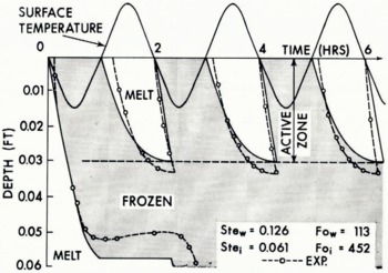
Fig. 2. Periodic freezing and thawing.
The classical Stefan solution, which is widely used in frost penetration studies, may be easily obtained from Equation (12) by putting ϕ s(τ) = 1. One of the obvious inadequacies of the solution is the neglect of property variations (Reference BrownBrown, 1964). Consider now the application of the “step” boundary condition to a domain in which the properties are spatially dependent. For this, the interface equation must be taken in the form

from which it is evident that the ease with which the integration may be performed depends upon the function of position contained in the product F 0 Ste. Writing this product as

it is evident that spatial dependency lies with the product ρL and to the greatest extent with L. A realistic variation of moisture content which will reveal the effect of this variation in a particular case is suggested from the measurements of Reference Crawford and LeggetCrawford 1961); these indicate a more or less exponential decay. Hence we will take F 0 Ste = A e ξ as a suitable relation at the interface. Substituting into Equation (12) and integrating yields
if ξ(τ 0) = τ 0 = 0. This compares with the constant-property solutions
based on the average moisture content, and
using the moisture content at the surface. The ratios τ/τ A and τ/τ M are shown plotted in Figure 3 from which it is evident that neglect of variation in moisture content can result in very large errors (in this case 20—100%) in estimating the time required to freeze a given depth (ξ = 1).

Fig. 3. Comparison of constant and spatially-dependent properties.
Temperature dependence of properties appears to be less important (Reference KerstenKersten, 1949), except perhaps for the problem resulting from a range of transition temperatures mentioned earlier. Reference Hamill and BankoffHamill and Bankoff (1964) have studied temperature-dependent properties but as yet no one appears to have considered the glaciological situation. Other than the transformation of the dependent variable, as given previously, there is no essential difference between handling temperature-dependent properties and spatially dependent properties in the asymptotic situation.
The Stefan solution for constant properties neglects the effect of conduction in the diminishing phase; this approximation is implicit in the form of Equation (12). The extent of the error involved may be determined by comparing the approximate solution for interface depth (ξ AP) with the exact solution (ξ EX) of Neumann (Reference Carslaw and JaegerCarslaw and Jaeger, 1959, p. 285) for a domain initially at a constant temperature θ 1 not equal to the fusion temperature. The discrepancy will depend upon the Stefan number and the ratio β = θ 1/θ c, where θ c is the step change at the surface. Figure 4 shows the ratio (ξ AP/ξ EX)−1 plotted against β for various values of Ste and reveals the fact that if β < 1 and Ste≪1 the approximation implied in Equation (12) is quite satisfactory.

Fig. 4. The effect of initial departure from the transition temperature.
When the temperature gradient at the surface is specified the asymptotic temperature distribution is more conveniently written in the form

so that the interface condition now becomes

Again, the form of ξ(τ) will depend upon the time dependency of ∂ϕ 0/∂x and the form of any property variation. For comparative purposes consider the case of a constant heat flux F at the surface of a constant-property medium for which we may take F 0 Ste ⋆ = 1, where

or, if ξ(τ 0) = τ 0 = 0,
This may be compared with a series solution (Reference Carslaw and JaegerCarslaw and Jaeger, 1959, p. 292) which, in our notation, is,
The history of the interface is described in Figure 5 for several values of Ste ⋆. The asymptotic solution once more reveals a tolerable error, in this case less than 7% if Ste ⋆ ≲ 0.8

Fig. 5. Interface history for constant heat flux.
4. Prescribed Convection
Melting of ice by convection at the boundary x = 0 will require satisfaction of the boundary condition

providing that sublimation or evaporation cause negligible movement of this plane. For simplicity, mass transfer will be ignored here, although it should be noted that its inclusion presents no special problems. The temperature distribution in the forming phase is given by Equation (13) and hence the interface condition is given by

or, since


Given any property dependency and the variation of Nu with time, integration of this equation provides the asymptotic solution for interface location. For the case of steady convection over a constant-property medium the integration is especially simple, giving
This agrees with the thermal circuit analysis of Reference London and SebanLondon and Seban (1943) (with ξ(τ 0) = τ 0 = 0). Figure 7 shows the interface location plotted against τ for various Nusselt numbers: when Nu → ∞, Equation (15) reduces to the Stefan solution as required. It is interesting to note that the curves in Figure 7 may be reduced to a single “universal” curve by simply multiplying Equation (15) by Nu. The function Nu ξ versus Nu 2 τ is shown in Figure 6 along with another approximate expression due to Reference BaxterBaxter (1962). Reference Carslaw and JaegerCarslaw and Jaeger (1959, p. 292) give the first two terms of a series solution to this problem, i.e.
in our notation. This approximates the curves shown in Figure 7 if Nu ξ ≪ 1 but is not complete enough for comparison at higher values.

Fig. 6. Interface history for constant convection.

Fig. 7. Parametric history for constant convection.
5. Prescribed Radiation
There are a good many situations in which incident or emitted thermal radiation plays an important, if not dominant, role in the history of an interface (Reference HoinkesHoinkes, 1955; Reference Schwerdtfeger and PounderSchwerdtfeger and Pounder, 1962; Reference LanglebenLangleben, 1966). Yet it appears that this situation has not been subjected to a theoretical attack. When heat exchange at the plane x = 0 is by radiation alone the boundary condition is conveniently written as

where in this special case, Ф = T/T c,
which, at x = 0, yields an algebraic equation for Φs(τ), i.e.
Typically, Gξ ≪ 1, and hence a solution of this equation may be sought by writing
and taking
Substituting in Equation (16) and grouping coefficients of like powers of Gξ gives an infinite set of algebraic equations for g 1, g 2, etc. Solving, we obtain

Hence,

If, for simplicity, we ignore incident radiation this reduces to
At the interface, Equation (6) (or (12) or (14)) becomes

if incident radiation is neglected and properties are constant. Rearranging,
and integrating
if ξ(τ 0) = τ 0 = 0. This “universal” relation is shown plotted in Figure 8 for each of the first four approximations to the left-hand side. Four terms appear to be adequate in describing the complete series. Figure 9 illustrates the effect of the “radiation number” on the interface history.

Fig. 8. Interface history for radiative cooling.

Fig. 9. Parametric history for radiative cooling.
6. Discussion and Conclusions
The asymptotic solutions developed above have been shown, wherever possible, to be close approximations to the truth for ice—water systems over a wide range of conditions. Despite their simplicity, these solutions reveal the essential characteristics of transition phenomena and are capable of generalization. For example, the constant-convection boundary condition yielded a relation of the form
which may be generalized immediately to
as confirmed by the complete solution for this case. Similarly, we may expect a general relation of the form Gξ = f 3(G 2 τ, Ste) for radiation.
The principal advantage of the asymptotic solution is the capacity to handle arbitrary boundary conditions. Typically, this advantage will outweigh the error resulting from the neglect of sensible heat effects, which are usually small. The results presented here are merely indicative of the procedure and the error involved. In general, the interface equation will be a first-order non-linear differential equation not soluble by elementary methods. Nevertheless, the equation may always be solved by fairly straight forward graphical or numerical methods to yield solutions for any meteorological condition at the surface and including any continuous spatial or temperature variation of the medium properties.
A representative assessment of the error implicit in the use of asymptotic solutions may be obtained from Figures 3 to 6. The error resulting from the neglect of property variations, as illustrated by Figure 3, may be considerably greater than those resulting from the use of an initial temperature not equal to the transition temperature or the neglect of sensible heat in the forming phase, as indicated by Figure 4. This last approximation, which is implicit in all asymptotic solutions, introduces an error of order not greater than Ste and typically much less.
In view of the wide range of situations in which an asymptotic solution may be of value it is virtually impossible to present separate results for each individual approximation involved. Regardless of the complexity of the situation, the normalization and subsequent order-ofmagnitude procedure should always provide an adequate measure of the validity of any particular approximation. It is suggested that most of those discussed in the paper would be of value within certain branches of the earth sciences and, in particular, within glaciology.
Acknowledgement
This work is part of a programme on ice formation sponsored by the National Research Council of Canada. The author would like to acknowledge the assistance of Mr C. S. Balasubramanian and Mrs P. Gillespie in the preparation of the illustrations.


