


Impact Statement
Data assimilation is the operational tool of choice when it comes to forecast Earth systems. The classical variational assimilation modeling framework is built on Gaussian prior hypothesis then relying on second-order statistics as hyperparameters, which may be hard to estimate. Inspired by deep image priors, we propose a hybrid method bridging a neural network and the 4D-Var mechanistic constraints to assimilate observation without specifying any statistics. It also constitutes a step toward bridging variational assimilation and deep learning, and extends the application domain of unlearned methods based on deep priors.
1. Introduction
Physics-driven numerical weather prediction requires estimating initial conditions before making a forecast. To do so, one should exploit all the knowledge at disposal which can be observations, a dynamical model, or errors statistics. It formalizes as an inverse problem and data assimilation offers a large panel of methods to solve it (Asch et al., Reference Asch, Bocquet and Nodet2016). A subset of these methods is variational so that the system state is estimated via the minimization of a cost function as in the 4D-Var algorithm (Le Dimet and Talagrand, Reference Le Dimet and Talagrand1986). Many similarities with machine learning have been highlighted (Abarbanel et al., Reference Abarbanel, Rozdeba and Shirman2018) as both can be used to perform Bayesian inversion by gradient descent.
Even though variational data assimilation has a long-standing experience in model-constrained optimization, deep learning techniques have revolutionized ill-posed inverse problem solving (Ongie et al., Reference Ongie, Jalal, Metzler, Baraniuk, Dimakis and Willett2020). And methods combining neural architectures and differentiable physical models already exist (Tompson et al., Reference Tompson, Schlachter, Sprechmann and Perlin2017; de Bezenac et al., Reference de Bezenac, Pajot and Gallinari2018; Mosser et al., Reference Mosser, Dubrule and Blunt2018). Most of the time, a large database is leveraged to learn a regularization adapted to the task.
Fitting observations respecting the dynamical model can be seen as a form of regularization but an additional regularizer may be required to promote an acceptable solution (Johnson et al., Reference Johnson, Hoskins and Nichols2005). Recently a very original idea called “deep prior” (Ulyanov et al., Reference Ulyanov, Vedaldi and Lempitsky2018) has been developed. A neural architecture is used to generate the solution of an inverse problem and acts like an implicit regularization. Astonishingly the whole architecture is trained in an unsupervised manner on one example and provides results comparable to supervised methods.
In this work, we propose a hybrid methodology bridging deep prior and variational data assimilation and we test it in a twin experiment. The algorithm is evaluated on an ocean-like motion estimation task requiring regularization, then compared to adapted data assimilation algorithms (Béréziat and Herlin, Reference Béréziat and Herlin2014, Reference Béréziat and Herlin2018). All algorithms are implemented using tools from the deep learning community. The code is available on GitHubFootnote 1.
2. Methodology
2.1. Data assimilation framework
A dynamical system is considered where a state
 $ \mathbf{X} $
evolves over time following perfectly-known dynamics
$ \mathbf{X} $
evolves over time following perfectly-known dynamics
 $ \unicode{x1D544} $
, see equation (1). Partial and noisy observations
$ \unicode{x1D544} $
, see equation (1). Partial and noisy observations
 $ \mathbf{Y} $
are available through an observation operator
$ \mathbf{Y} $
are available through an observation operator
 $ \unicode{x210D} $
, see equation (2). A background
$ \unicode{x210D} $
, see equation (2). A background
 $ {\mathbf{X}}_b $
gives prior information about the initial system state, see equation (3).
$ {\mathbf{X}}_b $
gives prior information about the initial system state, see equation (3).
 $$ \mathrm{Evolution}:\hskip1em {\mathbf{X}}_{t+1}={\unicode{x1D544}}_t\left({\mathbf{X}}_t\right), $$
 $$ \mathrm{Observation}:\hskip1em {\mathbf{Y}}_t={\unicode{x210D}}_t\left({\mathbf{X}}_t\right)+{\varepsilon}_{R_t}, $$
 $$ \mathrm{Background}:\hskip1em {\mathbf{X}}_0={\mathbf{X}}_B+{\varepsilon}_B. $$
Additive noise
 $ {\varepsilon}_B $
and
$ {\varepsilon}_B $
and
 $ {\varepsilon}_R $
represent uncertainties about the observations and the background, respectively. These noises are quantified by their assumed known covariance matrices
$ {\varepsilon}_R $
represent uncertainties about the observations and the background, respectively. These noises are quantified by their assumed known covariance matrices
 $ \mathbf{B} $
and
$ \mathbf{B} $
and
 $ \mathbf{R} $
, respectively. The dynamics is here considered perfect, but the framework could easily be extended to an imperfect dynamics. For any given matrix
$ \mathbf{R} $
, respectively. The dynamics is here considered perfect, but the framework could easily be extended to an imperfect dynamics. For any given matrix
 $ \mathbf{A} $
, we note
$ \mathbf{A} $
, we note
 $ \parallel x-y{\parallel}_A^2=\left\langle \left(x-y\right)|{\mathbf{A}}^{-1}\left(x-y\right)\right\rangle $
the associated Mahalanobis distance.
$ \parallel x-y{\parallel}_A^2=\left\langle \left(x-y\right)|{\mathbf{A}}^{-1}\left(x-y\right)\right\rangle $
the associated Mahalanobis distance.
2.2. Variational assimilation
The objective of data assimilation is to provide an estimation of the system state
 $ \mathbf{X} $
by optimally combining available data
$ \mathbf{X} $
by optimally combining available data
 $ {\mathbf{X}}_B $
,
$ {\mathbf{X}}_B $
,
 $ \mathbf{Y} $
and the dynamical model
$ \mathbf{Y} $
and the dynamical model
 $ \unicode{x1D544} $
. In the variational formalism (Le Dimet and Talagrand, Reference Le Dimet and Talagrand1986), this is done via the minimization of a cost function which is the sum of background errors and observational errors,
$ \unicode{x1D544} $
. In the variational formalism (Le Dimet and Talagrand, Reference Le Dimet and Talagrand1986), this is done via the minimization of a cost function which is the sum of background errors and observational errors,
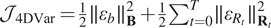 $ {\mathcal{J}}_{\hskip-0.1em 4\mathrm{DVar}}=\frac{1}{2}\parallel {\varepsilon}_b{\parallel}_{\mathbf{B}}^2+\frac{1}{2}{\sum}_{t=0}^T\parallel {\varepsilon}_{R_t}{\parallel}_{{\mathbf{R}}_t}^2 $
. The optimization problem is model-constrained as described in equation (4). What motivates this cost function is that minimizing it leads to the maximum a posteriori estimation of the state under independent Gaussian errors, linear observation operator, and linear model hypothesis. The corresponding optimization algorithm is named as 4D-Var.
$ {\mathcal{J}}_{\hskip-0.1em 4\mathrm{DVar}}=\frac{1}{2}\parallel {\varepsilon}_b{\parallel}_{\mathbf{B}}^2+\frac{1}{2}{\sum}_{t=0}^T\parallel {\varepsilon}_{R_t}{\parallel}_{{\mathbf{R}}_t}^2 $
. The optimization problem is model-constrained as described in equation (4). What motivates this cost function is that minimizing it leads to the maximum a posteriori estimation of the state under independent Gaussian errors, linear observation operator, and linear model hypothesis. The corresponding optimization algorithm is named as 4D-Var.
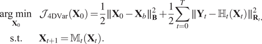 $$ {\displaystyle \begin{array}{cc}\underset{{\mathbf{X}}_0}{\arg \hskip0.22em \min }& {\mathcal{J}}_{\hskip-0.1em 4\mathrm{DVar}}\left({\mathbf{X}}_0\right)=\frac{1}{2}\parallel {\mathbf{X}}_0-{\mathbf{X}}_b{\parallel}_{\mathbf{B}}^2+\frac{1}{2}\sum \limits_{t=0}^T\parallel {\mathbf{Y}}_t-{\unicode{x210D}}_t\left({\mathbf{X}}_t\right){\parallel}_{{\mathbf{R}}_t,}^2\\ {}\mathrm{s}.\mathrm{t}.& \hskip-25em {\mathbf{X}}_{t+1}={\unicode{x1D544}}_t\left({\mathbf{X}}_t\right).\end{array}} $$
The link between variational assimilation and Tikhonov regularization is well described in Johnson et al. (Reference Johnson, Hoskins and Nichols2005). For example, choosing a particular matrix
 $ \mathbf{B} $
will promote a particular set of solutions. Therefore, making alike choices can be seen as a handcrafted regularization to take advantage of expert prior knowledge.
$ \mathbf{B} $
will promote a particular set of solutions. Therefore, making alike choices can be seen as a handcrafted regularization to take advantage of expert prior knowledge.
2.3. Deep prior 4D-Var
The idea behind deep prior is that using a well-suited neural architecture to generate a solution of the variational problem can act as a handcrafted regularization. This means that the control parameters are shifted from the system state space to the neural network parameters space. From a practical standpoint, a latent variable
 $ z $
is fixed and a generator network
$ z $
is fixed and a generator network
 $ {g}_{\theta } $
outputs the solution from it such that
$ {g}_{\theta } $
outputs the solution from it such that
 $ {g}_{\theta }(z)={\mathbf{X}}_0 $
.
$ {g}_{\theta }(z)={\mathbf{X}}_0 $
.
2.3.1. Cost function
The generator is then trained with the variational assimilation cost
 $ \mathcal{J}\left(\theta \right) $
. To emphasize the regularizing effect of the deep prior method, we choose to fix
$ \mathcal{J}\left(\theta \right) $
. To emphasize the regularizing effect of the deep prior method, we choose to fix
 $ \mathbf{B}=0 $
so that no background information is used. It means that
$ \mathbf{B}=0 $
so that no background information is used. It means that
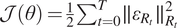 $ \mathcal{J}\left(\theta \right)=\frac{1}{2}{\sum}_{t=0}^T\parallel {\varepsilon}_{R_t}{\parallel}_{R_t}^2 $
and by denoting multiple integration between two times
$ \mathcal{J}\left(\theta \right)=\frac{1}{2}{\sum}_{t=0}^T\parallel {\varepsilon}_{R_t}{\parallel}_{R_t}^2 $
and by denoting multiple integration between two times
 $ {\unicode{x1D544}}_{t_1\to {t}_2} $
, the cost can be developed as in equation (5).
$ {\unicode{x1D544}}_{t_1\to {t}_2} $
, the cost can be developed as in equation (5).
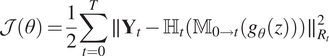 $$ \mathcal{J}\left(\theta \right)=\frac{1}{2}\sum \limits_{t=0}^T\parallel {\mathbf{Y}}_t-{\unicode{x210D}}_t\left({\unicode{x1D544}}_{0\to t}\left({g}_{\theta }(z)\right)\right){\parallel}_{R_t}^2 $$
It is important to note that this approach is unsupervised, the architecture being trained from scratch on one assimilation window with no pre-training. All the prior information should be contained in the architecture choice.
2.3.2. Gradient
The gradients of this cost function can be determined analytically. First, the chain rule gives equation (6). Then using the adjoint state method, we can develop
 $ {\nabla}_{{\mathbf{X}}_0}\mathcal{J}\left({\mathbf{X}}_0\right) $
as in equation (7), a detailed proof can be found in Asch et al. (Reference Asch, Bocquet and Nodet2016). In the differentiable programming paradigm, such analytical expression is not needed to obtain gradients, adjoint modeling is implicitly performed as gradients are backpropagated automatically.
$ {\nabla}_{{\mathbf{X}}_0}\mathcal{J}\left({\mathbf{X}}_0\right) $
as in equation (7), a detailed proof can be found in Asch et al. (Reference Asch, Bocquet and Nodet2016). In the differentiable programming paradigm, such analytical expression is not needed to obtain gradients, adjoint modeling is implicitly performed as gradients are backpropagated automatically.
 $$ {\nabla}_{\theta}\mathcal{J}\left(\theta \right)={\nabla}_{{\mathbf{X}}_0}\mathcal{J}\left({\mathbf{X}}_0\right){\nabla}_{\theta }{\mathbf{X}}_0={\nabla}_{{\mathbf{X}}_0}\mathcal{J}\left({\mathbf{X}}_0\right){\nabla}_{\theta }{g}_{\theta }(z) $$
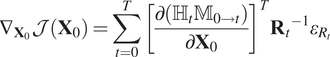 $$ {\nabla}_{{\mathbf{X}}_0}\mathcal{J}\left({\mathbf{X}}_0\right)=\sum \limits_{t=0}^T{\left[\frac{\partial \left({\unicode{x210D}}_t{\unicode{x1D544}}_{0\to t}\right)}{\partial {\mathbf{X}}_0}\right]}^T{{\mathbf{R}}_t}^{-1}{\varepsilon}_{R_t} $$
2.3.3. Algorithm
The algorithm seeks to numerically optimize the cost function and simply consists of alternating forward and backward integration to update the control parameters by gradient descent (see Algorithm 1). A schematic view of the forward integration can be found in Figure 1.
Algorithm 1 – Deep prior 4D-Var.
Initialize fixed latent variables
 $ z $
.
$ z $
.
Initialize control variables
 $ \theta $
.
$ \theta $
.
while stop criterion do.
forward: integrate
 $ {\unicode{x1D544}}_{0\to T}\left({g}_{\theta }(z)\right) $
and compute
$ {\unicode{x1D544}}_{0\to T}\left({g}_{\theta }(z)\right) $
and compute
 $ \mathcal{J} $
.
$ \mathcal{J} $
.
backward: automatic differentiation returns
 $ {\nabla}_{\theta}\mathcal{J} $
.
$ {\nabla}_{\theta}\mathcal{J} $
.
update:
 $ \theta =\mathrm{optimizer}\left(\theta, \mathcal{J},{\nabla}_{\theta}\mathcal{J}\right) $
.
$ \theta =\mathrm{optimizer}\left(\theta, \mathcal{J},{\nabla}_{\theta}\mathcal{J}\right) $
.
end while.
return
 $ \theta, {\mathbf{X}}_0 $
.
$ \theta, {\mathbf{X}}_0 $
.
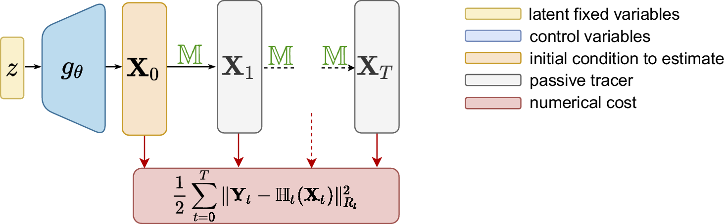
Figure 1. Schematic view of the forward integration in deep prior 4D-Var.
3. Case Study
3.1. Twin experiment
The proposed methodology is tested within a twin experiment where data are generated from a numerical dynamical model. Observations are then created by sub-sampling and adding noise. The aim of this experiment is to highlight the implicit regularizing effect of the deep generative network. To do so, we compare various algorithms on the observation assimilation task. The considered algorithms are 4D-Var with no regularization, 4D-Var with Tikhonov regularization, and deep prior 4D-Var. All the algorithms are implemented with tools based on automatic differentiation such that no adjoint modeling is required, as described in Filoche et al. (Reference Filoche, Béréziat, Brajard and Charantonis2021). In all the assimilation experiments, the dynamical model is perfectly known.
3.2. Dynamical system
3.2.1. State
State variables of the considered system are
 $ \eta $
, the height deviation of the horizontal pressure surface from its mean height, and
$ \eta $
, the height deviation of the horizontal pressure surface from its mean height, and
 $ \mathbf{w} $
, the associated velocity field.
$ \mathbf{w} $
, the associated velocity field.
 $ \mathbf{w} $
can be decomposed in
$ \mathbf{w} $
can be decomposed in
 $ u $
and
$ u $
and
 $ v $
, the zonal and meridional velocity, respectively. At each time
$ v $
, the zonal and meridional velocity, respectively. At each time
 $ t $
, the system state is then
$ t $
, the system state is then
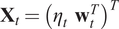 $ {\mathbf{X}}_t={\left({\eta}_t\hskip0.5em {\mathbf{w}}_t^T\right)}^T $
. The considered temporal window has a fixed size.
$ {\mathbf{X}}_t={\left({\eta}_t\hskip0.5em {\mathbf{w}}_t^T\right)}^T $
. The considered temporal window has a fixed size.
3.2.2. Shallow water model
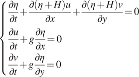
The dynamical model used here corresponds to a discretization of the shallow water equations system in equation (8) with first-order upwind numerical schemes. These schemes are implemented using a natively differentiable software.
 $ H $
represents the mean height of the horizontal pressure surface and
$ H $
represents the mean height of the horizontal pressure surface and
 $ g $
the acceleration due to gravity. After reaching an equilibrium starting from Gaussian random initial conditions, system trajectories are simulated as shown in Figure 2.
$ g $
the acceleration due to gravity. After reaching an equilibrium starting from Gaussian random initial conditions, system trajectories are simulated as shown in Figure 2.
 $$ \left\{\begin{array}{l}\frac{\partial \eta }{\partial t}+\frac{\partial \left(\eta +H\right)u}{\partial x}+\frac{\partial \left(\eta +H\right)v}{\partial y}=0\\ {}\frac{\partial u}{\partial t}+g\frac{\partial \eta }{\partial x}=0\\ {}\frac{\partial v}{\partial t}+g\frac{\partial \eta }{\partial y}=0\end{array}\right. $$
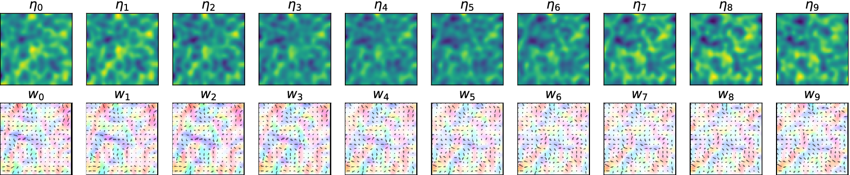
Figure 2. Example of simulated trajectory with the shallow water numerical model.
3.2.3. Observations
At regular observational dates,
 $ \eta $
is fully observed up to an additive white noise, see Figure 3. The velocity field
$ \eta $
is fully observed up to an additive white noise, see Figure 3. The velocity field
 $ \mathbf{w} $
is never observed. This means that at observational date
$ \mathbf{w} $
is never observed. This means that at observational date
 $ t $
, the observation operator
$ t $
, the observation operator
 $ {\unicode{x210D}}_t $
is then a linear projector so that
$ {\unicode{x210D}}_t $
is then a linear projector so that
 $ {\eta}_t={\unicode{x210D}}_t{\mathbf{X}}_t $
.
$ {\eta}_t={\unicode{x210D}}_t{\mathbf{X}}_t $
.
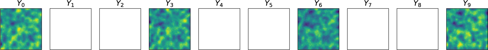
Figure 3. Example of simulated system observations.
3.3. Regularization
The role of the assimilation task is then to estimate the velocity field from successive observations of
 $ \eta $
. Such motion estimation inverse problem can be ill-posed and may need regularization. The dynamical model being considered perfect, all the velocity fields within the window are determined by the initial field
$ \eta $
. Such motion estimation inverse problem can be ill-posed and may need regularization. The dynamical model being considered perfect, all the velocity fields within the window are determined by the initial field
 $ {\mathbf{w}}_0 $
.
$ {\mathbf{w}}_0 $
.
3.3.1. No regularization
The 4D-Var version without regularization only optimizes the fit-to-data term in the cost function. This means that no prior knowledge on the solution can be used and the background covariance matrix
 $ \mathbf{B} $
vanishes.
$ \mathbf{B} $
vanishes.
3.3.2. Tikhonov regularization
On the other hand, the “Tikhonov” 4D-Var algorithm optimizes the fit-to-data term and also a penalty term. The estimated motion field is forced to be smooth by constraining
 $ \parallel \nabla {\mathbf{w}}_0{\parallel}_2^2 $
and
$ \parallel \nabla {\mathbf{w}}_0{\parallel}_2^2 $
and
 $ \parallel \nabla .{\mathbf{w}}_0{\parallel}_2^2 $
to be small. As proved in Lepoittevin and Herlin (Reference Lepoittevin and Herlin2016), these terms can be directly included in the background error using a particular matrix
$ \parallel \nabla .{\mathbf{w}}_0{\parallel}_2^2 $
to be small. As proved in Lepoittevin and Herlin (Reference Lepoittevin and Herlin2016), these terms can be directly included in the background error using a particular matrix
 $ \mathbf{B} $
such that
$ \mathbf{B} $
such that
 $ \alpha \parallel \nabla {\mathbf{w}}_0{\parallel}_2^2+\beta \parallel \nabla .{\mathbf{w}}_0{\parallel}_2^2=\parallel {\mathbf{X}}_0-{\mathbf{X}}_b{\parallel}_{B_{\alpha, \beta}}^2 $
, where
$ \alpha \parallel \nabla {\mathbf{w}}_0{\parallel}_2^2+\beta \parallel \nabla .{\mathbf{w}}_0{\parallel}_2^2=\parallel {\mathbf{X}}_0-{\mathbf{X}}_b{\parallel}_{B_{\alpha, \beta}}^2 $
, where
 $ \alpha $
and
$ \alpha $
and
 $ \beta $
are the parameters to be tuned. Such regularization is a classical optical flow penalty (Horn and Schunck, Reference Horn and Schunck1981) and can be used for the sea-surface circulation estimation (Béréziat, Reference Bereziat, Herlin and Younes2000, Béréziat and Herlin, Reference Béréziat and Herlin2014).
$ \beta $
are the parameters to be tuned. Such regularization is a classical optical flow penalty (Horn and Schunck, Reference Horn and Schunck1981) and can be used for the sea-surface circulation estimation (Béréziat, Reference Bereziat, Herlin and Younes2000, Béréziat and Herlin, Reference Béréziat and Herlin2014).
3.3.3. Deep prior
As depicted in the method, the only assumption made is about the architecture of the network
 $ {g}_{\theta } $
generating the solution
$ {g}_{\theta } $
generating the solution
 $ {\mathbf{w}}_0 $
. Obviously, the chosen architecture is critical for performance. In this experiment, we use the generative convolutional architecture introduced by Radford et al. (Reference Radford, Metz and Chintala2016), but replacing deconvolution operations to avoid checkerboard artifacts as described in Odena et al. (Reference Odena, Dumoulin and Olah2016). The exact architecture is provided in Appendix A.1, Figure 6.
$ {\mathbf{w}}_0 $
. Obviously, the chosen architecture is critical for performance. In this experiment, we use the generative convolutional architecture introduced by Radford et al. (Reference Radford, Metz and Chintala2016), but replacing deconvolution operations to avoid checkerboard artifacts as described in Odena et al. (Reference Odena, Dumoulin and Olah2016). The exact architecture is provided in Appendix A.1, Figure 6.
3.3.4. Hyperparameters tuning
Regarding 4D-Var,
 $ \alpha $
and
$ \alpha $
and
 $ \beta $
are tuned using Bayesian optimization on observations forecasts so that ground truth is never used. Finding hyperparameters, and particularly the number of epochs for DIP is still an active research field as described in Wang et al. (Reference Wang, Li, Zhuang, Chen, Liang and Sun2021). Investigated early-stopping methods are beyond the scope of our study so we made the choice to fix the number of epochs.
$ \beta $
are tuned using Bayesian optimization on observations forecasts so that ground truth is never used. Finding hyperparameters, and particularly the number of epochs for DIP is still an active research field as described in Wang et al. (Reference Wang, Li, Zhuang, Chen, Liang and Sun2021). Investigated early-stopping methods are beyond the scope of our study so we made the choice to fix the number of epochs.
4. Results
The first result to look at is the plot of the velocity fields estimated by the algorithms (Figure 4, 7). The 2D field of arrows represents the direction and the intensity of the velocity, the colormap provides the same information but helps visualization. Without regularization, the 4D-Var estimation is sharp and seems to suffer from numerical optimization artifacts. On the contrary, the deep prior estimate looks less precise but far smoother. The regularized provides the most accurate and smooth estimation. Other examples can be found in Appendix A.2.
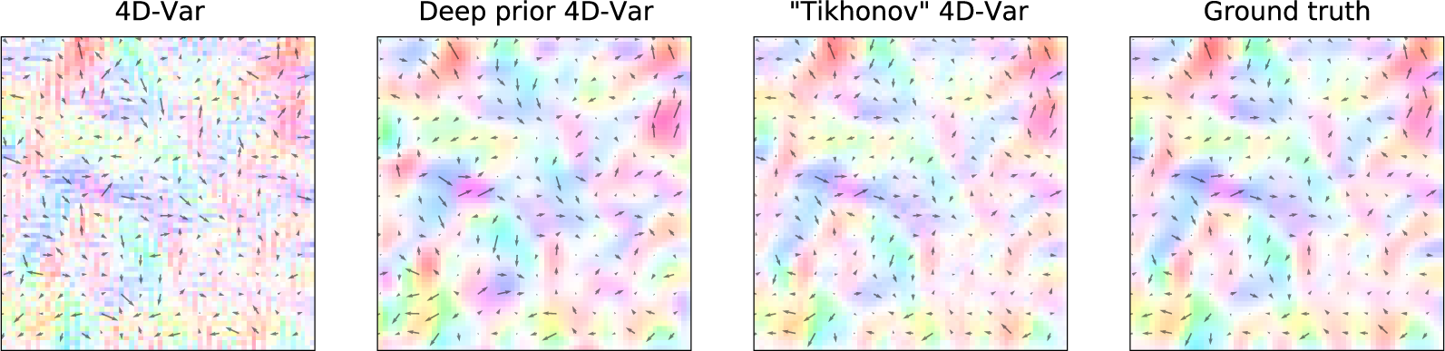
Figure 4. Example of the estimated motion fields
 $ {\mathbf{w}}_0 $
with various algorithms.
$ {\mathbf{w}}_0 $
with various algorithms.
Several metrics are calculated to quantify the quality of the estimations. The endpoint error
 $ \parallel {\hat{\mathbf{w}}}_0-{\mathbf{w}}_0{\parallel}_2 $
and the angular error
$ \parallel {\hat{\mathbf{w}}}_0-{\mathbf{w}}_0{\parallel}_2 $
and the angular error
 $ \operatorname{arccos}\Big({\hat{\mathbf{w}}}_0,{\mathbf{w}}_0 $
) are classical optical flow scores, they calculate the Euclidean distance and the average angular deviation between the estimation and the ground truth, respectively. At first glance, there is no statistical difference between deep prior 4D-Var and 4D-Var without regularization (Table 1).
$ \operatorname{arccos}\Big({\hat{\mathbf{w}}}_0,{\mathbf{w}}_0 $
) are classical optical flow scores, they calculate the Euclidean distance and the average angular deviation between the estimation and the ground truth, respectively. At first glance, there is no statistical difference between deep prior 4D-Var and 4D-Var without regularization (Table 1).
Table 1. Metrics quantifying the quality of the estimated motion field
 $ {\mathbf{w}}_0 $
over the assimilated database.
$ {\mathbf{w}}_0 $
over the assimilated database.

a All the metrics are averaged on images, ± precising standard deviation.
However, if we dig into the smoothness statistics of the estimated fields,
 $ \parallel \nabla .{\mathbf{w}}_0{\parallel}_2 $
,
$ \parallel \nabla .{\mathbf{w}}_0{\parallel}_2 $
,
 $ \parallel \nabla .{\mathbf{w}}_0{\parallel}_2 $
, and
$ \parallel \nabla .{\mathbf{w}}_0{\parallel}_2 $
, and
 $ \parallel \Delta {\mathbf{w}}_0{\parallel}_2 $
, it seems that deep prior is able to capture complex statistics of the true motion field. Similar behavior has been noticed in Yoo et al. (Reference Yoo, Jin, Gupta, Yerly, Stuber and Unser2021)). Looking closer at the histograms, Figure 5, we see that deep prior and “Tikhonov” 4D-Var estimations have smoothness statistics very close to that of the original motion field. Whether it has been explicitly constrained or by deep network design, smooth solutions are unforced by regularization.
$ \parallel \Delta {\mathbf{w}}_0{\parallel}_2 $
, it seems that deep prior is able to capture complex statistics of the true motion field. Similar behavior has been noticed in Yoo et al. (Reference Yoo, Jin, Gupta, Yerly, Stuber and Unser2021)). Looking closer at the histograms, Figure 5, we see that deep prior and “Tikhonov” 4D-Var estimations have smoothness statistics very close to that of the original motion field. Whether it has been explicitly constrained or by deep network design, smooth solutions are unforced by regularization.
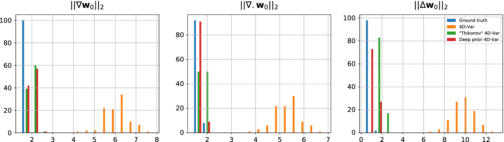
Figure 5. Histograms of smoothness statistics from the estimated motion field
 $ {\mathbf{w}}_0 $
with various algorithms.
$ {\mathbf{w}}_0 $
with various algorithms.
It has to be noted that the “Tikhonov” 4D-Var is the only algorithm here that has been treated with hyperparameters tuning which can explain the large differences in scores. It can be argued that the neural architecture, which is known as a good baseline to generate images, has been tuned through many image processing experiments. However, grid-searching hyperparameters particularly suited for this experiment should enhance performances.
5. Conclusion
We proposed an original method bridging ideas from the image processing and the geosciences communities to solve a variational inverse problem. More precisely, we used a neural network as implicit regularization to generate the solution of an initial value problem. To demonstrate its efficiency, we set up a twin experiment comparing different algorithms in a data assimilation task derived from the shallow water model. The results show that this kind of regularization can provide an interesting alternative when prior knowledge is not available. However, in our case, we observed that expert-driven handcrafted regularization provides better performances. Finally, this work opens the way for further developments on the architecture design, but also in a more realistic context where the numerical dynamics is imperfect.
Author Contributions
Conceptualization: all authors; Data visualization: A.F.; Methodology: A.F.; Project administration: D.B., A.C.; Writing—original draft: A.F.; Writing—review and editing: all authors. All authors approved the final submitted draft.
Competing Interests
The authors declare no competing interests exist.
Data Availability Statement
Data are synthetic, all experiments are reproducible through the GitHub repository provided by the authors.
Ethics Statement
The research meets all ethical guidelines, including adherence to the legal requirements of the study country.
Funding Statement
This research was supported by Sorbonne Center for Artificial Intelligence.
Provenance
This article is part of the Climate Informatics 2022 proceedings and was accepted in Environmental Data Science on the basis of the Climate Informatics peer review process.
A. Appendix. Experiment details
A.1. Neural network architecture
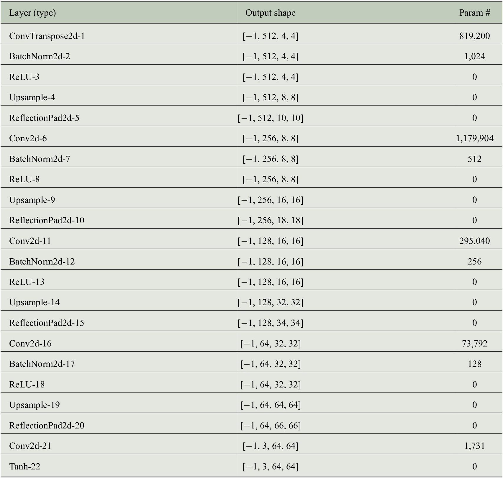
Trainable params: 2,371,587.
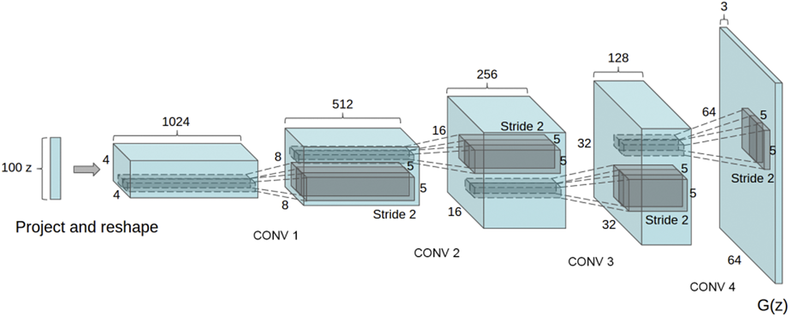
Figure 6. The convolutional generator architecture from Radford et al. (Reference Radford, Metz and Chintala2016).
A.2. Supplementary examples
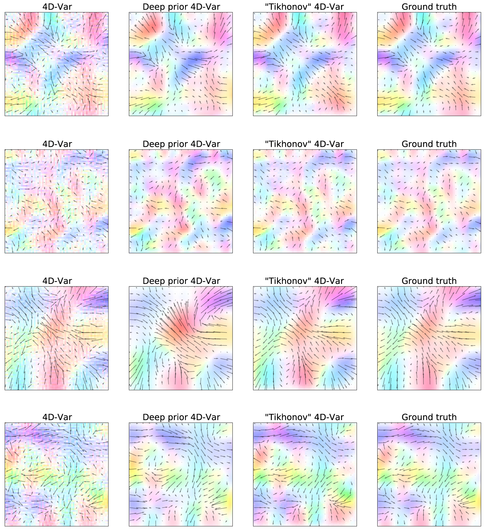
Figure 7. Examples of the estimated motion fields
 $ {\mathbf{w}}_0 $
with various algorithms, each line corresponds to a different assimilation window.
$ {\mathbf{w}}_0 $
with various algorithms, each line corresponds to a different assimilation window.


 Open access