


1. Introduction
Mobile manipulation is a popular topic in robotics research due to the omnipresence of this task in robotic applications. From home assistance [Reference Huang, Tanie and Sugano1] to Mars exploration [Reference Howard and Kelly2], mobile manipulators find application in a variety of domains. To further expand their utility in uncontrolled outdoor environments, significant research effort has been allocated to increasing the resiliency of mobile manipulators to their operating environment. Among numerous harshness that can arise in outdoor environments, terrain variation [Reference Papadopoulos and Rey3] is one of the most common, and it can be dangerously harmful to the performance of a mobile robot if rollover or sliding occurs.
Heavy machines commonly used in mining, logging, and construction, such as excavators, feller bunchers, and loaders, can also be treated as mobile manipulators. Due to the slow progress of automation in these industries, the issues related to terrain variation and its effect on the machine operation have rarely been addressed in mobile manipulation research. The aforementioned machines are prone to roll over as they have a high center of mass, manipulate heavy objects, and inevitably have to operate on slopes and in adverse weather conditions. The prevention of rollover and sliding is critical, as such failures pose numerous risks to the operator, machine, as well as the environment; these considerations provide the main motivation for the present work.
To ensure the upright stability of robots during mobile manipulation, passive methods such as novel mechanical design [Reference Lindroos, La Hera and Haggstrom4, Reference Chen, Kamezaki, Katano, Kaneko, Azuma, Ishida, Seki, Ichiryu and Sugano5] and steep slope avoidance [Reference Pai and Reissell6, Reference Ge and Cui7] can be utilized. However, the former solution does not address the needs of machine designs currently employed in the field, and slope avoidance is simply not a viable solution for applications such as steep slope logging. Therefore, in this article, we propose a framework to plan the trajectory and reconfiguration of a mobile manipulator robot under dynamic stability constraint so that a robot of common design can access its work areas in rough terrain with safety assurance. Before the proposed approach is presented, past literature on stability measures, stability-constrained trajectory planning, and autonomous industrial machines is reviewed.
1.1. Stability measures
Several measures designed to quantify proximity to rollover through force/moment measurements include the measure that relies on static force and moment analysis introduced in ref. [Reference Gibson, Elliott and Persson8], the force-angle stability measure in refs. [Reference Papadopoulos and Rey3, Reference Diaz-Calderon and Kelly9, Reference Mosadeghzad, Naderi and Ganjefar10], and the lateral load transfer parameter employed in refs. [Reference Bouton, Lenain, Thuilot and Fauroux11, Reference Bouton, Lenain, Thuilot and Martinet12, Reference Denis, Thuilot and Lenain13]. However, these measures are based on the forces/moments experienced at joints or wheels and cannot provide direct guidelines for trajectory planning. For humanoid robots, the zero moment point (ZMP) stability measure was introduced in ref. [Reference Vukobratovic and Stepanenko14] to achieve quantitative stability inference based on joint motions and robot inertia parameters. Since mobile manipulation planning has to account for the robot’s and the manipulated object’s inertia parameters and the robot’s joint motions, the ZMP stability measure is naturally chosen for our work.
An early implementation of the ZMP measure for a mobile manipulator is presented in ref. [Reference Sugano, Huang and Kato15], and further work on mobile robots with stability constraint evolved from it. Guided by the ZMP formulation, a mobile manipulator’s base generates stability-compensating motions, while the manipulator arm is executing tasks [Reference Huang, Tanie and Sugano1, Reference Dine, Corrales-Ramon, Mezouar and Fauroux16]. By using potential functions derived from the ZMP formulation, stability-compensating motion can also be generated for manipulator arms, as demonstrated in refs. [Reference Kim, Chung, Youm and Lee17, Reference Lee, Park and Lee18, Reference Choi and Oh19, Reference Lee, Leibold, Buss and Park20]. However, requiring a mobile manipulator robot to continuously generate motion that compensates for stability during operations will reduce the robot’s efficiency for task completion; ideally, stability-compensating motion should only occur when rollover risk is imminent. This approach also assumes that the robot has enough control authority to maintain balance on the path.
The ZMP measure has also been transformed into linear state inequality constraints in Model Predictive Control (MPC) formulations for the special cases of a car-like [Reference Stankiewicz, Brown and Brennan21] and a forklift-like [Reference Mohammadi, Mareels and Oetomo22] mobile robot operating on planar surface. Nonetheless, in rough terrain applications, the ZMP measure linearization cannot be generalized, and it can be impossible to find a trajectory satisfying the stability constraint along a path that was generated without accounting for stability apriori. Considering the limitations in the aforementioned recent works that address ZMP-constrained trajectory planning [Reference Dine, Corrales-Ramon, Mezouar and Fauroux16, Reference Choi and Oh19, Reference Stankiewicz, Brown and Brennan21], we next review previous work on constrained mobile manipulation planning in general.
1.2. Constrained mobile manipulation trajectory planning
The trajectory planning problem of a mobile manipulator robot under a kinodynamic constraint such as the ZMP constraint can be solved, at least in theory, by using two types of planning methods: sampling-based methods [Reference LaValle and Kuffner23, Reference Wang, Meng and Khatib24] and optimization-based methods [Reference Shin and McKay25, Reference Bobrow, Dubowsky and Gibson26, Reference Seraji27, Reference Verschueren, van Duijkeren, Swevers and Diehl28, Reference Castillo-Lopez, Ludivig, Sajadi-Alamdari, Sanchez-Lopez, Olivares-Mendez and Voos29]. A sampling-based method can generate motion trajectories by randomly sampling the search space, and it can accommodate discrete dynamics and any nonlinear constraint. An optimization-based method involves constructing a nonlinear optimal control problem (NOCP) from a user-defined cost and constraint functions.
However, the time complexity of a sampling-based approach becomes impractically high when the search space includes accelerations, especially for high DoF systems such as mobile manipulators. As a result, previous works utilized sampling-based methods [Reference LaValle and Kuffner23, Reference Wang, Meng and Khatib24] to only address the path generation problem. On the other hand, for an NOCP structure, the nonlinearities in robot kinematics and constraints make it difficult to directly obtain a solution for the trajectory in a timely manner because the associated nonlinear programming scheme relies heavily on a good initial guess to arrive at a feasible optimum. Hence, none of the previously reported NOCP-based solutions [Reference Shin and McKay25, Reference Bobrow, Dubowsky and Gibson26, Reference Seraji27, Reference Verschueren, van Duijkeren, Swevers and Diehl28] can be applied to solve our problem since they focused on generating trajectories, given an existing path. A recent NOCP-based work that addresses path and trajectory planning with dynamic obstacle avoidance [Reference Castillo-Lopez, Ludivig, Sajadi-Alamdari, Sanchez-Lopez, Olivares-Mendez and Voos29] only demonstrated computation efficiency for a potential field (PF) formulation under constant obstacle velocity assumption; this method cannot accommodate dynamic stability constraints such as the ZMP constraint due to their non-convexity and the fact that constant velocity assumptions do not hold in our case.
A hierarchical planning structure solves the trajectory planning problem by breaking it down into multiple stages to exponentially reduce the problem dimensionality and to take advantage of both the versatile sampling-based methods and the mathematically efficient optimization-based methods. Under the hierarchical structure, sampling-based path planners, such as the Rapidly-exploring Random Tree (RRT) [Reference LaValle and Kuffner23] method, can efficiently address quasi-static path planning problems under nonlinear kinematic and state constraints. The NOCP-based trajectory generation can then be warm-started by using the quasi-static path as a “close enough” initial guess.
In recent years, hierarchical planning has been used with some success in autonomous driving and for UAVs, as demonstrated in refs. [Reference Cowlagi and Tsiotras30, Reference Li, Sun, Cao, He and Zhu31, Reference Lim, Lee, Sunwoo and Jo32, Reference Shao, He, Zhao and Wu33]. However, the aforementioned hierarchical planning examples only apply to the specific applications they were designed for and cannot accommodate the dynamic stability constraint. Hence, the need for a hierarchical framework specifically designed to address the mobile manipulator rough terrain trajectory planning problem is justified.
1.3. Robotics in timber harvesting
Timber harvesting, which is the targeted application of our work, is a very important industry for many countries including Canada. The majority of modern timber harvesting businesses worldwide employ feller bunchers and timber harvesters to fell trees, and use skidders and forwarders to transport felled trees for further processing. The aforementioned machines can be considered as a type of mobile manipulator since they consist of mobile bases and hydraulically powered mechanized arms with multiple degrees of freedom. Nowadays, the machines still fully rely on operator’s judgment and control in order to function [Reference Lindroos, La Hera and Haggstrom4]. However, with operator shortages in the forecast, there is a strong impetus for developing an autonomous harvesting system.
Some progress has been made to increase the timber harvesting machines’ autonomy. The dynamics model of a timber harvester is presented in ref. [Reference Papadopoulos and Sarkar34]; the teleoperation of a forestry manipulator is showcased in ref. [Reference Westerberg, Manchester, Mettin, Hera and Shiriaev35]; the hydraulic actuator control of a forwarder machine has been discussed in refs. [Reference Hera, Mettin, Westerberg and Shiriaev36] and [Reference Morales, Westerberg, La Hera, Freidovich and Shiriaev37], and the motion control of a forestry manipulator along a fixed path is presented in ref. [Reference Morales, Hera, Westerberg, Freidovich and Shiriaev38]. However, a versatile trajectory planning algorithm that can handle the terrain-related challenges of timber harvesting is yet to be developed. Therefore, the goal of this paper is to introduce a method that addresses the issue of stability-constrained mobile manipulation path and trajectory planning problem, inspired by the operational requirements on the timber harvesting machinery.
1.4. About this paper
Encompassing our earlier work in ref. [Reference Song and Sharf39] that mainly deals with online dynamic-stability-constrained manipulation planning, the framework presented in this paper consists of the following main advances compared to existing result in the literature:
-
• The dynamic-stability-constrained time-optimal trajectory planning is formulated and solved as a hierarchical planning problem for mobile manipulation on varying 3D terrain.
-
• The proposed hierarchical framework allows for both path and trajectory generation online and utilizes the manipulator arm’s reconfiguration capability to traverse steeper terrain.
-
• A theoretical analysis of the ZMP measure is provided to allow for modifications to sampling-based path planning algorithms so that satisfaction of the non-convex ZMP constraint is guaranteed in continuous motion.
-
• To ensure the NOCP is “warm-started” with a feasible initial guess, the ZMP-constrained quasi-static trajectory is proven to have guaranteed finite completion time.
Thanks to the hierarchical framework, online planning computation is achieved. To the best of the authors’ knowledge, the framework presented in this paper is the first to enable point-to-point 3D terrain mobile manipulation planning with a focus on time-optimal task completion, rather than stability compensation along pre-existing path. In other words, a stability measure acts as a constraint that does not interfere with the robot’s task execution unless the constraint is violated. In addition to computational efficiency, the benefits of the proposed framework include the ability to utilize manipulator reconfiguration for rough terrain traverse and to generate locally time-optimal motions, as compared to previous works [Reference Huang, Tanie and Sugano1, Reference Dine, Corrales-Ramon, Mezouar and Fauroux16, Reference Kim, Chung, Youm and Lee17, Reference Choi and Oh19, Reference Lee, Leibold, Buss and Park20] which mainly focus on generating motions to compensate for stability.
In this paper, a feller buncher machine employed for timber harvesting is considered as a mobile manipulator robot. For the remainder of the paper and previously, the term reconfiguration refers to changes in the manipulator pose; the term relocation refers to changes in the position and heading direction of the mobile base; quasi-static path refers to a trajectory with sufficiently low velocity so that it can be considered as a geometric path. At any point on the quasi-static path, the robot can be treated as a static, as opposed to dynamic system, the former descriptor implying zero velocities and accelerations. Onwards, the paper is organized as follows.
In Section 2, kinematics model of the machine, the ZMP measure, and the NOCP formulation to solve the dynamic-stability-constrained trajectory planning problem are introduced as theoretical background for the paper. In Section 3, the dynamic-stability-constrained manipulation planning problem is addressed through dimension reduction for online computation. In Section 4, online rough terrain mobile relocation planning under dynamic stability constraint is addressed by employing a hierarchical framework. The relationship and interaction between the local manipulation planner and the relocation planner are illustrated in Fig. 1. Simulation results showcasing the proposed motion planning framework will be presented in Section 5; that Section also includes a qualitative comparison to another NOCP-based approach, and a quantitative comparison to the popular MPC path following solution. Conclusions and future work will be stated in Section 6.

Figure 1. Overview of local manipulation problem and relocation planning problem.
2. Theoretical background
2.1. System model and ZMP constraint
We first derive the full kinematic model of a mobile manipulator (a.k.a., system), an example of which is shown schematically in Fig. 2 (left). The manipulator arm of the robot has
 $n \in \mathbb{Z}^{0+}$
joint DoFs, and the mobile base is modeled as a unicycle on arbitrary, but known terrain. A unicycle model is commonly used to represent the kinematics of differential drive robots and skid-steered machines [Reference Siciliano, Sciavicco, Villani and Oriolo40], which is the case of the feller buncher.
$n \in \mathbb{Z}^{0+}$
joint DoFs, and the mobile base is modeled as a unicycle on arbitrary, but known terrain. A unicycle model is commonly used to represent the kinematics of differential drive robots and skid-steered machines [Reference Siciliano, Sciavicco, Villani and Oriolo40], which is the case of the feller buncher.

Figure 2. On the left, schematic diagram of a tracked mobile manipulator with 5 manipulator DoFs; the three axes of each link frame
 $\textbf{x}_i$
,
$\textbf{x}_i$
,
 $\textbf{y}_i$
, and
$\textbf{y}_i$
, and
 $\textbf{z}_i$
are represented by red, green, and blue arrows, respectively. On the right, rectangular support polygon
$\textbf{z}_i$
are represented by red, green, and blue arrows, respectively. On the right, rectangular support polygon
 $Conv(S)$
.
$Conv(S)$
.
Frame
 $\mathcal{O}$
is the inertial frame, and frame
$\mathcal{O}$
is the inertial frame, and frame
 $\mathcal{F}_i$
is fixed to the
$\mathcal{F}_i$
is fixed to the
 $i$
-th link of the robot for
$i$
-th link of the robot for
 $i\in \{0,1,\ldots,n\}$
. Here, link
$i\in \{0,1,\ldots,n\}$
. Here, link
 $0$
refers to the robot’s mobile base, links
$0$
refers to the robot’s mobile base, links
 $1$
to
$1$
to
 $n-1$
refer to the manipulator arm components, and link
$n-1$
refer to the manipulator arm components, and link
 $n$
refers to the robot’s end effector. We denote the angle of joint
$n$
refers to the robot’s end effector. We denote the angle of joint
 $i$
between link
$i$
between link
 $i-1$
and
$i-1$
and
 $i$
with
$i$
with
 $q_i\in \mathbb{R}$
(
$q_i\in \mathbb{R}$
(
 $i = 1,2,\ldots,n$
) and collect all joint angles into a column vector
$i = 1,2,\ldots,n$
) and collect all joint angles into a column vector
 $\textbf{q}\in \mathbb{R}^n$
. We consider the base-fixed frame
$\textbf{q}\in \mathbb{R}^n$
. We consider the base-fixed frame
 $\mathcal{F}_0$
to undergo translation, as measured with
$\mathcal{F}_0$
to undergo translation, as measured with
 $\textbf{p}_b^{\mathcal{O}}$
, and a
$\textbf{p}_b^{\mathcal{O}}$
, and a
 $\textbf{z}$
-
$\textbf{z}$
-
 $\textbf{x}$
-
$\textbf{x}$
-
 $\textbf{y}$
rotation from initial attitude through angles
$\textbf{y}$
rotation from initial attitude through angles
 $\psi$
(yaw),
$\psi$
(yaw),
 $\theta$
(pitch), and
$\theta$
(pitch), and
 $\phi$
(roll), respectively; this allows the base to be located on arbitrary-sloped terrain. The generalized coordinates of the base and the manipulator are assembled in
$\phi$
(roll), respectively; this allows the base to be located on arbitrary-sloped terrain. The generalized coordinates of the base and the manipulator are assembled in
 $\bar{\textbf{q}} = \left[\textbf{p}_b^{\mathcal{O}^T}, \psi, \theta, \phi, \textbf{q}^T\right]^T$
. Then, defining
$\bar{\textbf{q}} = \left[\textbf{p}_b^{\mathcal{O}^T}, \psi, \theta, \phi, \textbf{q}^T\right]^T$
. Then, defining
 $\textbf{x} = \left[\bar{\textbf{q}}^T, \dot{\bar{\textbf{q}}}^T\right]^T$
, the mobile manipulator’s kinematics equations can be written in state space form as:
$\textbf{x} = \left[\bar{\textbf{q}}^T, \dot{\bar{\textbf{q}}}^T\right]^T$
, the mobile manipulator’s kinematics equations can be written in state space form as:
 \begin{equation} \dot{\textbf{x}} = g(\textbf{x},\textbf{u}). \end{equation}
where we introduced the kinematic control input
 $\textbf{u}=\left[u_a,u_\psi,\textbf{u}_q^T\right]^T$
, with
$\textbf{u}=\left[u_a,u_\psi,\textbf{u}_q^T\right]^T$
, with
 $u_a$
,
$u_a$
,
 $u_\psi$
, and
$u_\psi$
, and
 $\textbf{u}_q$
as accelerations along heading direction, yaw angular acceleration, and manipulator arm joint accelerations, respectively. Eq. (1) serves as the model of the robot for the overall optimal trajectory planning problem. Note that the terrain information is embedded in (1) through the orientation of the base.
$\textbf{u}_q$
as accelerations along heading direction, yaw angular acceleration, and manipulator arm joint accelerations, respectively. Eq. (1) serves as the model of the robot for the overall optimal trajectory planning problem. Note that the terrain information is embedded in (1) through the orientation of the base.
In addition to the kinematics Eq. (1), a geometric construction called the support polygon will be used throughout this paper. The support polygon, denoted by
 $Conv(S)$
, is a convex hull formed by the contact points between the robot’s mobile base and the ground (see Fig. 2, right.)
$Conv(S)$
, is a convex hull formed by the contact points between the robot’s mobile base and the ground (see Fig. 2, right.)
The ZMP measure, central to this paper, allows to quantify the rollover stability margin of a mobile manipulator on arbitrary terrain using only its kinematic model and inertia parameters, instead of full dynamics model or force measurements. It is therefore our method of choice due to the potential benefit of faster trajectory planning calculations and its practicality. To compute the ZMP location, we define the Cartesian coordinates of each component’s center of mass relative to
 $\textbf{p}_b$
expressed in
$\textbf{p}_b$
expressed in
 $\mathcal{F}_0$
as
$\mathcal{F}_0$
as
 $\textbf{p}_i^{\mathcal{F}_0} = [x_i,y_i,z_i]^T$
and the corresponding accelerations
$\textbf{p}_i^{\mathcal{F}_0} = [x_i,y_i,z_i]^T$
and the corresponding accelerations
 $\ddot{\textbf{p}}_i^{\mathcal{F}_0} = [\ddot x_i,\ddot y_i,\ddot z_i]^T$
. By employing kinematics, these can be obtained from:
$\ddot{\textbf{p}}_i^{\mathcal{F}_0} = [\ddot x_i,\ddot y_i,\ddot z_i]^T$
. By employing kinematics, these can be obtained from:
 \begin{equation} \begin{aligned} \textbf{p}_i^{\mathcal{F}_0}& = \textbf{f}_i(\bar{\textbf{q}}) \\[5pt] \ddot{\textbf{p}}_i^{\mathcal{F}_0} &= \dot{\textbf{J}}_{pi}(\bar{\textbf{q}})\dot{\bar{\textbf{q}}}+\textbf{J}_{pi}(\bar{\textbf{q}})\ddot{\bar{\textbf{q}}}, \end{aligned} \end{equation}
where we introduced the position kinematics Jacobian,
 $\textbf{J}_{pi}(\bar{\textbf{q}})=\dfrac{\partial{\textbf{f}_i}}{\partial{\bar{\textbf{q}}}}$
. Then, according to ref. [Reference Sugano, Huang and Kato15] and using the gravitational vector
$\textbf{J}_{pi}(\bar{\textbf{q}})=\dfrac{\partial{\textbf{f}_i}}{\partial{\bar{\textbf{q}}}}$
. Then, according to ref. [Reference Sugano, Huang and Kato15] and using the gravitational vector
 $\textbf{g}^{\mathcal{F}_0} = [g_x,g_y,g_z]^T$
, the coordinates of the ZMP in the base frame
$\textbf{g}^{\mathcal{F}_0} = [g_x,g_y,g_z]^T$
, the coordinates of the ZMP in the base frame
 $\textbf{p}_{\text{zmp}}^{\mathcal{F}_0} = [x_{\text{zmp}}, y_{\text{zmp}}, 0]^T$
are given byFootnote 1:
$\textbf{p}_{\text{zmp}}^{\mathcal{F}_0} = [x_{\text{zmp}}, y_{\text{zmp}}, 0]^T$
are given byFootnote 1:
 \begin{equation} \begin{aligned} x_{\text{zmp}} &= \dfrac{\sum _{i=0}^n m_i(\ddot{z}_i-g_z)x_i-\sum _{i=0}^n m_i(\ddot{x}_i-g_x) z_i}{\sum _{i=0}^n m_i(\ddot{z}_i-g_z)}\\[5pt] y_{\text{zmp}} &= \dfrac{\sum _{i=0}^n m_i(\ddot{z}_i-g_z)y_i-\sum _{i=0}^n m_i(\ddot{y}_i-g_y) z_i}{\sum _{i=0}^n m_i(\ddot{z}_i-g_z)}. \end{aligned} \end{equation}
Note, by definition, ZMP lies in the plane of the support polygon so that its z-coordinate in
 $\mathcal{F}_0$
is zero. Also, the mass of the manipulated object, assumed to be known in this work, can be easily accounted for in (3). The robot is dynamically (ZMP-) stable when the constraint
$\mathcal{F}_0$
is zero. Also, the mass of the manipulated object, assumed to be known in this work, can be easily accounted for in (3). The robot is dynamically (ZMP-) stable when the constraint
 $\textbf{p}_{\text{zmp}}\in Conv(S)$
is satisfied; it has a tendency to rollover otherwise. Equation (3) can be evaluated by substituting from the kinematics equations (2), once the base and the manipulator motions have been planned, to produce the ZMP locus, that is, the trajectory of ZMP in
$\textbf{p}_{\text{zmp}}\in Conv(S)$
is satisfied; it has a tendency to rollover otherwise. Equation (3) can be evaluated by substituting from the kinematics equations (2), once the base and the manipulator motions have been planned, to produce the ZMP locus, that is, the trajectory of ZMP in
 $\mathcal{F}_0$
during the motion of the robot. The ZMP stability constraint is a major contributor to the high computational cost when enforced in optimal control formulations as it is nonlinear and non-convex with respect to the system’s states.
$\mathcal{F}_0$
during the motion of the robot. The ZMP stability constraint is a major contributor to the high computational cost when enforced in optimal control formulations as it is nonlinear and non-convex with respect to the system’s states.
2.2. Optimal control problem formulation
We consider this problem in full generality by allowing the robot to be situated on slopes of different grades. With the view to optimizing the efficiency of manipulation tasks, the motions should be carried out within the shortest possible time, without the robot rolling over. Naturally, to minimize the overall time required for the robot to reach final state
 $\textbf{x}_f$
from an initial state
$\textbf{x}_f$
from an initial state
 $\textbf{x}_0$
safely, we formulate a constrained NOCP of the form:
$\textbf{x}_0$
safely, we formulate a constrained NOCP of the form:
 \begin{equation} \begin{aligned} \min _{\textbf{u}} \;\;&\int _{t_0}^{t_f} 1\; \text{d} t.\\[5pt] \text{s.t.}\;\;& \dot{\textbf{x}}=g(\textbf{x},\textbf{u})\;\;\textbf{x}(t_0) = \textbf{x}_0\;\;\textbf{x}(t_f) = \textbf{x}_f\\[5pt] &\textbf{p}_{\text{zmp}}(\textbf{x},\textbf{u})\in Conv(S)\\[5pt] &\underline{\textbf{x}} \leq \textbf{x}\leq \overline{\textbf{x}}\\[5pt] &\underline{\textbf{u}} \leq \textbf{u}\leq \overline{\textbf{u}}, \end{aligned} \end{equation}
where
 $\preccurlyeq$
is defined as vector component-wise inequality,
$\preccurlyeq$
is defined as vector component-wise inequality,
 $\underline{\textbf{x}}$
and
$\underline{\textbf{x}}$
and
 $\overline{\textbf{x}}$
stand for the lower and upper bounds on the system state
$\overline{\textbf{x}}$
stand for the lower and upper bounds on the system state
 $\textbf{x}$
, and
$\textbf{x}$
, and
 $\underline{\textbf{u}}$
and
$\underline{\textbf{u}}$
and
 $\overline{\textbf{u}}$
stand for the lower and upper bounds on the control input
$\overline{\textbf{u}}$
stand for the lower and upper bounds on the control input
 $\textbf{u}$
, respectively. The state and input constraints ensure that the robot’s configuration, rates, and accelerations are realistic and therefore feasible when tracked; we also point out the inclusion of the ZMP stability constraint in (4).
$\textbf{u}$
, respectively. The state and input constraints ensure that the robot’s configuration, rates, and accelerations are realistic and therefore feasible when tracked; we also point out the inclusion of the ZMP stability constraint in (4).
Problem (4) is a NOCP with standard initial and final state constraints and the additional non-convex path constraint to enforce ZMP stability. Without pre-defined constraint arc sequence and boundaries (i.e., no a priori knowledge of ZMP-constrained motion occurrence), the optimality condition becomes impossible to formulate, and indirect formulations that aim to approach optimality conditions cannot be applied [Reference Betts41]. Hence, the two-point boundary value problem constructed from the NOCP problem has to be solved with a direct formulation using numerical methods, such as the shooting method.
Additionally, because of the nonlinear terrain function and the highly nonlinear ZMP constraint, the numerical methods must rely on a “close enough” initialization to find a solution in reasonable time [Reference Guibout and Scheeres42]. Since finding an appropriate initialization is a nontrivial task, it is impossible to solve (4) reliably using existing solution techniques for NOCP alone. To address this issue, the rough terrain mobile manipulation problem will be decomposed into two sub-problems: a robot arm manipulation planning problem and a mobile base relocation planning problem. Further, the dimension reduction technique to speed up the manipulation planning solution will be introduced in Section 3, and the techniques involved with generating the quasi-static path to warm start the relocation planning will be introduced in Section 4.
3. Manipulation planning under dynamic stability constraint with simplified kinematics
A common task for a mobile manipulator is to interact with objects by securing, lifting, and placing them at a location either nearby or at a distance. When dissected into two general modes of operation – mobile relocation and local manipulation – any mobile manipulation task can be defined as a combination of these two modes, either taking place simultaneously or separately. Therefore, it is desirable to solve the two stages separately in order to avoid the computational burden caused by a high-dimensional NOCP.
The local manipulation planning of the mobile manipulator robot is addressed in this section. During this stage, the robot has to execute joint motions in order to reconfigure itself or interact with an object. The dynamic stability of the robot is likely to be compromised when the robot has high center of mass, when the joint motions are aggressive, when the terrain is steep, and when the object is heavy. Trajectory planning for the mobile relocation stage will be introduced in Section 4.
Due to the high dimensionality of the kinematics model (1), the nonlinearity that resides in the forward kinematics equations (2) and the ZMP formulation (3), the solution of the optimal manipulation planning problem (4) requires longer than practical computation time for online guidance, even for a case where the base does not move. In order to develop an online trajectory planner for the robot, a model simplification is called upon.
To simplify the optimal control problem by reducing the dimensionality of the problem, and considering typical modes of operation such as of a feller buncher in timber harvesting or excavators in mining and construction, the
 $n$
-DoF manipulator arm is simplified to have 2 DoFs including the first link yaw angle
$n$
-DoF manipulator arm is simplified to have 2 DoFs including the first link yaw angle
 $q_1(t)$
and variable end effector distance
$q_1(t)$
and variable end effector distance
 $d(t)$
from the yaw joint axis. The simplified model is illustrated schematically in Fig. 3. For local manipulation planning only, the following assumptions are made:
$d(t)$
from the yaw joint axis. The simplified model is illustrated schematically in Fig. 3. For local manipulation planning only, the following assumptions are made:

Figure 3. Schematic diagram of a simplified mobile manipulator.
Assumption 1. (a) The mobile base has a fixed attitude and accelerates along
 $\textbf{y}_0$
direction. (b) The
$\textbf{y}_0$
direction. (b) The
 $z$
-coordinate (height) of end effector does not change in
$z$
-coordinate (height) of end effector does not change in
 $\mathcal{F}_0$
. (c) The inverse kinematics mapping between end effector distance
$\mathcal{F}_0$
. (c) The inverse kinematics mapping between end effector distance
 $d$
and full model arm joint angles
$d$
and full model arm joint angles
 $\textbf{q}$
except for
$\textbf{q}$
except for
 $q_1$
is known up to the second order derivative with respect to time.
$q_1$
is known up to the second order derivative with respect to time.
The reductions in computation costs resulting from the use of the simplified model will be demonstrated in Section 5.2. Note that in practice, local manipulation tasks such as picking and placing rarely require complex movements of the mobile base, Assumption 1(a) can be justified for cases such as excavation and timber harvesting. A formulation that allows the execution of complex mobile maneuvers is presented in Section 4 in the context of a relocation problem. To mitigate the limitations caused by Assumption 1(b), a specially designed motion planner can manipulate the end effector into or out of the
 $x$
-
$x$
-
 $y$
plane of
$y$
plane of
 $\mathcal{F}_0$
, without significant loss in performance as the vertical movements required are usually small. Assumption 1(c) is easily satisfied as inverse kinematics resolution method mentioned in ref. [Reference Reiter, Müller and Gattringer43] is well established.
$\mathcal{F}_0$
, without significant loss in performance as the vertical movements required are usually small. Assumption 1(c) is easily satisfied as inverse kinematics resolution method mentioned in ref. [Reference Reiter, Müller and Gattringer43] is well established.
In the simplified model, the control inputs are
 $u_{q_1}$
, acceleration of
$u_{q_1}$
, acceleration of
 $q_1$
, and
$q_1$
, and
 $u_d$
, the second derivative of
$u_d$
, the second derivative of
 $d$
with respect to time. The kinematics model of the simplified model is straightforward to derive and can be written in state space form:
$d$
with respect to time. The kinematics model of the simplified model is straightforward to derive and can be written in state space form:
 \begin{equation} \dot{\tilde{\textbf{x}}} = \tilde{g}(\tilde{\textbf{x}},\tilde{\textbf{u}}), \end{equation}
where
 $\tilde{\textbf{x}} = [q_1,\dot{q}_1,d,\dot{d}]^T$
, and
$\tilde{\textbf{x}} = [q_1,\dot{q}_1,d,\dot{d}]^T$
, and
 $\tilde{\textbf{u}} = [u_{q_1}, u_d]$
.
$\tilde{\textbf{u}} = [u_{q_1}, u_d]$
.
To ensure that the ZMP location of the full model follows that of the simplified model, a mapping between the DoFs of the simplified model and those of the full model of the robot needs to be established. From Assumption 1(c), the robot’s joint angles, angular rates, and accelerations can be expressed using the states and control inputs of the simplified model as:
 \begin{equation} \begin{aligned} \textbf{q}&=[q_1, \mathcal{IK}(d)]^T\\[5pt] \dot{\textbf{q}}&=[\dot{q}_1, \mathcal{IK}^1(\dot{d},d)]^T\\[5pt] \ddot{\textbf{q}}&=[u_{q_1}, \mathcal{IK}^2(u_d,\dot{d},d)]^T. \end{aligned} \end{equation}
Here,
 $\mathcal{IK}$
represents the inverse kinematics mapping referred to in Assumption 1(c) equation and the superscript signifies its order of derivative with respect to time. Therefore, using the mapping provided in (1), (3), and (6), the ZMP location of the full kinematics model can be expressed using the simplified kinematic quantities
$\mathcal{IK}$
represents the inverse kinematics mapping referred to in Assumption 1(c) equation and the superscript signifies its order of derivative with respect to time. Therefore, using the mapping provided in (1), (3), and (6), the ZMP location of the full kinematics model can be expressed using the simplified kinematic quantities
 $\tilde{\textbf{x}}$
and
$\tilde{\textbf{x}}$
and
 $\tilde{\textbf{u}}$
as
$\tilde{\textbf{u}}$
as
 $\tilde{\textbf{p}}_{\text{zmp}}(\tilde{\textbf{x}},\tilde{\textbf{u}})$
.
$\tilde{\textbf{p}}_{\text{zmp}}(\tilde{\textbf{x}},\tilde{\textbf{u}})$
.
To shorten the computational time so that the trajectory planner can provide online guidance, the full kinematic model (1) is replaced by the simplified kinematic model (5) in the optimal control problem (4). It is noted that although the kinematic model’s dimension has been reduced, the ZMP constraint is still derived from (3) using information of all joints obtained from (6). Hence, the motions generated by solving the NOCP with the simplified model will guarantee ZMP constraint satisfaction for the full model. Also, we point out that in employing the simplified model, the dimension of the NOCP kinematic constraints has been reduced from
 $2n+12$
to
$2n+12$
to
 $4$
, and the number of control inputs has been reduced from
$4$
, and the number of control inputs has been reduced from
 $n+2$
to
$n+2$
to
 $2$
. However, the input constraints can no longer be placed directly on joint accelerations, although in practice, this can be resolved by tightening the bound on
$2$
. However, the input constraints can no longer be placed directly on joint accelerations, although in practice, this can be resolved by tightening the bound on
 $\bar{\textbf{u}}$
until all joint accelerations are feasible. We also note that the control bounds are considered to be independent from terrain.
$\bar{\textbf{u}}$
until all joint accelerations are feasible. We also note that the control bounds are considered to be independent from terrain.
4. Rough terrain relocation planning
In this section, dynamic-stability-constrained trajectory planning of the relocation stage of mobile manipulation is addressed. During relocation, a mobile manipulator has to navigate a constantly undulating terrain and, sometimes, shift its ZMP through reconfiguring the manipulator to safely move through steep slope. As noted earlier, the topographic map of the 3D terrain, as well as the goal point for the robot are assumed to be known.
To solve this problem, a hierarchical planning framework that consists of a sampling-based planning level and a NOCP solution level is proposed. The framework relies on the sampling-based planning to first conduct quasi-static path and reconfiguration planning. The quasi-static result is then used as an initial guess to warm start the NOCP level (4) for fast computation.
As defined in previous works [Reference Dalibard, Khoury, Lamiraux, Nakhaei, Taïx and Laumond44] and [Reference Ardakani, Bimbo and Prattichizzo45], quasi-static planning considers a robot to have near zero velocity and acceleration so that the kinodynamic constraints of the path planning problem can be simplified to static constraints. A disadvantage of the quasi-static planning is that it does not provide any guarantees on constraint satisfaction under dynamic conditions. As a result, the path has to be followed by the robot at slow speed to avoid constraint violation. Hence, the latter NOCP level is added to form the proposed hierarchical framework and to generate safe dynamic trajectories.
Algorithm 1 ZMP-constrained path planning

4.1. Quasi-static path planning algorithm
Sampling-based approach is chosen to solve the path and reconfiguration planning problem due to its theoretical completeness, ability to deal with nonlinear constraints, and efficiency when search space is purposefully constructed. The sampling-based planning structure used in our implementation is based on the RRT algorithm proposed in ref. [Reference LaValle and Kuffner23]. The pseudo-code of what we call “RRT
 $\mathcal{S}$
” is shown in Algorithm 1, and it includes two main modifications: the first to accommodate the ZMP stability constraint on line 9 highlighted in blue and the second modification made to allow manipulator reconfiguration, lines 13-14 highlighted in red. The RRT algorithm, specifically, is chosen due to its ability to quickly find a path when new terrain and obstacles such as human, fallen trees, or large rocks appear on the map. However, the ZMP constraint accommodation can also be directly implemented within other sampling-based planning algorithms.
$\mathcal{S}$
” is shown in Algorithm 1, and it includes two main modifications: the first to accommodate the ZMP stability constraint on line 9 highlighted in blue and the second modification made to allow manipulator reconfiguration, lines 13-14 highlighted in red. The RRT algorithm, specifically, is chosen due to its ability to quickly find a path when new terrain and obstacles such as human, fallen trees, or large rocks appear on the map. However, the ZMP constraint accommodation can also be directly implemented within other sampling-based planning algorithms.
4.1.1. Stability guarantee
Since the sampling-based algorithm only checks constraint satisfaction at every sampling point, it does not guarantee that the constraints are met between sampling points. To ensure the sampling-based algorithm generates a quasi-static path that is guaranteed to be ZMP-stable in continuous execution, the
 $\text{ZMPStable}$
function on line 9 of Algorithm 1 checks that the stability conditions to be introduced in Section 4.3 are met.
$\text{ZMPStable}$
function on line 9 of Algorithm 1 checks that the stability conditions to be introduced in Section 4.3 are met.
4.1.2. Reconfiguration
To reduce the search space dimension for online path generation with RRT, the robot is considered to be quasi-statically moving through the terrain. As the path planning tree growth reaches the steep Section in a terrain map, new nodes will become less likely to be added to the tree. This is due to stability constraints becoming harder to satisfy. To remedy this problem, random joint reconfiguration is executed whenever the number of new nodes added to the tree is lower than a threshold after certain number of iterations, as indicated in lines 13 and 14 of Algorithm 1. In this way, the robot will be able to navigate through steep slopes by reconfiguring its arm. The method introduced in Section 3 is used to further plan the motion trajectory of each reconfiguration. In this manner, our implementation is designed to allow for exploration of the robot’s configuration space for higher mobility on rough terrain without unnecessarily reconfiguring at every sampling point.
4.2. Finite-time feasibility guarantee
Due to the quasi-static nature of the path planning stage, the inertial terms in the ZMP constraints are ignored. Therefore, a quasi-static path generated with Algorithm 1 does not guarantee that there exists a trajectory for the robot to travel to its destination without violating the dynamic stability constraint when the robot’s components experience non-zero linear and angular accelerations. In order to address this issue, the following theorem is introduced:
Theorem 4.1. For a robot with unicycle kinematics traveling along a geometric path
 $\tau \;:\; I \to \textbf{x}$
, where
$\tau \;:\; I \to \textbf{x}$
, where
 $I=[0,1]$
is a unit interval, if the ZMP location
$I=[0,1]$
is a unit interval, if the ZMP location
 $\textbf{p}_{zmp}(\tau )$
belongs to the interior of
$\textbf{p}_{zmp}(\tau )$
belongs to the interior of
 $Conv(S)\;\forall \;\tau$
,
$Conv(S)\;\forall \;\tau$
,
 $\exists$
 $\textbf{u}$
for the constrained trajectory planning problem (4) such that
$\textbf{u}$
for the constrained trajectory planning problem (4) such that
 $t_f=T\lt \lt \infty$
.
$t_f=T\lt \lt \infty$
.
A proof of Theorem 4.1 is provided in Appendix A. With Theorem 4.1 backing, the method to find a quasi-static path that satisfies the ZMP constraint is presented in the following subsections. It is worth pointing out that Theorem 4.1 also shows that a ZMP-constrained quasi-static path is a controlled invariant set of robot state
 $\textbf{x}$
as defined in ref. [Reference Blanchini46].
$\textbf{x}$
as defined in ref. [Reference Blanchini46].
4.3. Stability-guaranteed sampling-based path search for continuous motion
To plan a robot path on 3D terrain using a sampling-based algorithm, such as RRT, nonlinear constraints are checked at each sampling point to ensure constraint violations do not occur. However, to keep the computation time reasonable, constraint satisfaction cannot be verified continuously in between sampling points. Since the ZMP constraint (3) is non-convex with respect to the robot’s base orientation, even if the robot is dynamically stable at two neighboring sampling points, it is not guaranteed to be dynamically stable between two sampling points. To resolve this issue, an analytical method to determine the ZMP stability between sampling points is desired.
In the stability-constrained RRT implementation, ZMP constraint satisfaction is unchecked in the following two scenarios. The first is when the robot’s base changes its heading direction at a particular sampling location and the second is the robot quasi-statically “slides” from one sampling location to the next. Since the two instances happen separately in the RRT implementation, they can be dealt with individually. In the following analysis, we will make use of
 $g_z\gt 0$
, since we do not expect the robot to drive up vertical walls. In addition, under the quasi-static condition, (3) reduces to
$g_z\gt 0$
, since we do not expect the robot to drive up vertical walls. In addition, under the quasi-static condition, (3) reduces to
 \begin{equation} x_{\text{zmp}} = \dfrac{M_x g_z-M_z g_x}{M g_z},\;\; y_{\text{zmp}} = \dfrac{M_y g_z-M_z g_y}{M g_z}, \end{equation}
where
 $M_x=\sum _i m_i x_i$
,
$M_x=\sum _i m_i x_i$
,
 $M_y=\sum _i m_i y_i$
,
$M_y=\sum _i m_i y_i$
,
 $M_z=\sum _i m_i z_i$
, and
$M_z=\sum _i m_i z_i$
, and
 $M=\sum _i m_i$
. When the same robot is located on the horizontal terrain, according to (7), its ZMP location is further simplified to:
$M=\sum _i m_i$
. When the same robot is located on the horizontal terrain, according to (7), its ZMP location is further simplified to:
 \begin{equation} x_{\text{zmp,0}}=\frac{M_x}{M},\;\; y_{\text{zmp,0}}=\frac{M_y}{M}. \end{equation}
4.3.1. Mobile base attitude
To analyze the ZMP stability of the two aforementioned scenarios, we first need to define the robot base attitude on arbitrary 3D terrain. With
 $\textbf{p}_b=[s_x, s_y, s_z]^T$
representing the 3D coordinate of terrain surface in inertial frame
$\textbf{p}_b=[s_x, s_y, s_z]^T$
representing the 3D coordinate of terrain surface in inertial frame
 $\mathcal{O}$
at the location of the mobile base, the terrain can be expressed by the following nonlinear function:
$\mathcal{O}$
at the location of the mobile base, the terrain can be expressed by the following nonlinear function:
 \begin{equation} s_z = h(s_x, s_y). \end{equation}
Let us denote the rotation matrix that describes the attitude change of the base-fixed frame
 $\mathcal{F}_0$
from the inertial frame
$\mathcal{F}_0$
from the inertial frame
 $\mathcal{O}$
as
$\mathcal{O}$
as
 $R=\{r_{ij}\}\;(i,j = 1,2,3)$
, and since the base-fixed
$R=\{r_{ij}\}\;(i,j = 1,2,3)$
, and since the base-fixed
 $z_0$
axis of a mobile manipulator remains perpendicular to terrain surface under normal operations, defining the directional gradients of the terrain
$z_0$
axis of a mobile manipulator remains perpendicular to terrain surface under normal operations, defining the directional gradients of the terrain
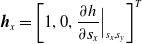 $\textbf{h}_x = \left [1,0,\dfrac{\partial h}{\partial s_x}\Bigr |_{s_x,s_y}\right ]^T$
and
$\textbf{h}_x = \left [1,0,\dfrac{\partial h}{\partial s_x}\Bigr |_{s_x,s_y}\right ]^T$
and
 $\textbf{h}_y = \left [0,1,\dfrac{\partial h}{\partial s_y}\Bigr |_{s_x,s_y}\right ]^T$
, the third column of
$\textbf{h}_y = \left [0,1,\dfrac{\partial h}{\partial s_y}\Bigr |_{s_x,s_y}\right ]^T$
, the third column of
 $R$
can be represented as:
$R$
can be represented as:
 \begin{equation*} \hat {\textbf{r}}_3 = \frac {\textbf{h}_x \times \textbf{h}_y}{\left |\left | \textbf{h}_x \times \textbf{h}_y \right | \right |}. \end{equation*}
Let us denote the heading angle defined by the projection of the mobile base’s heading vector onto the 2-D plane
 $\textbf{x}_{\mathcal{O}}$
-
$\textbf{x}_{\mathcal{O}}$
-
 $\textbf{y}_{\mathcal{O}}$
as
$\textbf{y}_{\mathcal{O}}$
as
 $\bar{\psi }$
. The second column of
$\bar{\psi }$
. The second column of
 $R$
describes the mobile base’s heading direction on the 3D surface and can then be written as:
$R$
describes the mobile base’s heading direction on the 3D surface and can then be written as:
 \begin{equation*} \hat {\textbf{r}}_2 = \frac {[\textbf{h}_x, \textbf{h}_y]\left[\!-\!\sin {\bar {\psi }}, \cos {\bar {\psi }}\right]^T}{\left |\left |[\textbf{h}_x, \textbf{h}_y]\left[\!-\!\sin {\bar {\psi }}, \cos {\bar {\psi }}\right]^T\right |\right |}. \end{equation*}
Hence, the first column of
 $R$
can be found using:
$R$
can be found using:
 \begin{equation*} \hat {\textbf{r}}_1 = \frac { \hat {\textbf{r}}_2 \times \hat {\textbf{r}}_3}{\left |\left | \hat {\textbf{r}}_2 \times \hat {\textbf{r}}_3\right |\right |}. \end{equation*}
4.3.2. Stability guarantee during base turn
Inspecting (7), it is clear that
 $g_x$
,
$g_x$
,
 $g_y$
, and
$g_y$
, and
 $g_z$
are the only quantities that vary with the robot’s orientation. As a robot whose attitude is described by the rotation matrix
$g_z$
are the only quantities that vary with the robot’s orientation. As a robot whose attitude is described by the rotation matrix
 $R$
executes a skid-steered turn through angle
$R$
executes a skid-steered turn through angle
 $\psi ^t$
, the gravity components are affected by the yaw angle
$\psi ^t$
, the gravity components are affected by the yaw angle
 $\psi ^t$
and can be expressed as:
$\psi ^t$
and can be expressed as:
 \begin{equation} \begin{aligned} \begin{bmatrix} g^t_x\\[5pt] g^t_y\\[5pt] g^t_z \end{bmatrix}&= \begin{bmatrix} \cos{\psi ^t}&\sin{\psi ^t}&0\\[5pt] -\!\sin{\psi ^t}&\cos{\psi ^t}&0\\[5pt] 0&0&1 \end{bmatrix} \underbrace{\begin{bmatrix} \hat{\textbf{r}}_1^T\\[5pt] \hat{\textbf{r}}_2^T\\[5pt] \hat{\textbf{r}}_3^T \end{bmatrix}}_{R^T} \begin{bmatrix} 0\\[5pt]0\\[5pt]g \end{bmatrix}\\[5pt] &=\begin{bmatrix} r_{13}\cos{\psi ^t}g+r_{23}\sin{\psi ^t}g\\[5pt] -r_{13}\sin{\psi ^t}g+r_{23}\cos{\psi ^t}g\\[5pt] r_{33}g \end{bmatrix}. \end{aligned} \end{equation}
The ZMP after the turn is then found from:
 \begin{equation} x^t_{\text{zmp}} = \dfrac{M_x g^t_z-M_z g^t_x}{M g^t_z},\; y^t_{\text{zmp}} = \dfrac{M_y g^t_z-M_z g^t_y}{M g^t_z}. \end{equation}
To aid in the illustration of stability guarantee during a skid-steered turn, the following claim is presented with a proof that follows:
Proposition 1.
As a wheeled/tracked robot executes a continuous unidirectional quasi-static turn through angle
 $\psi ^t$
about its yaw axis, the ZMP of the robot traces, monotonically on the support polygon, an arc of angle
$\psi ^t$
about its yaw axis, the ZMP of the robot traces, monotonically on the support polygon, an arc of angle
 $\psi ^t$
, radius
$\psi ^t$
, radius
 $\dfrac{r_{13}^2M_z^2+r_{23}^2M_z^2}{r_{33}^2M^2}$
, and center
$\dfrac{r_{13}^2M_z^2+r_{23}^2M_z^2}{r_{33}^2M^2}$
, and center
 $[x_{\text{zmp,0}},\;y_{\text{zmp,0}}]^T$
.
$[x_{\text{zmp,0}},\;y_{\text{zmp,0}}]^T$
.
Proof 1. By defining
 $\Delta x_{\text{zmp}}=x^t_{\text{zmp}}-x_{\text{zmp,0}}$
, and
$\Delta x_{\text{zmp}}=x^t_{\text{zmp}}-x_{\text{zmp,0}}$
, and
 $\Delta y_{\text{zmp}}=y^t_{\text{zmp}}-y_{\text{zmp,0}}$
, the difference between (11) and (8) can be represented as:
$\Delta y_{\text{zmp}}=y^t_{\text{zmp}}-y_{\text{zmp,0}}$
, the difference between (11) and (8) can be represented as:
 \begin{equation} \Delta x_{\text{zmp}} = \frac{M_zg^t_x}{-Mg^t_z}, \;\; \Delta y_{\text{zmp}} = \frac{M_zg^t_y}{-Mg^t_z}. \end{equation}
Substituting (10) into (12), we obtain
 \begin{equation} \begin{bmatrix} \Delta x_{\text{zmp}}\\[5pt] \Delta y_{\text{zmp}} \end{bmatrix} = \begin{bmatrix} \cos{\psi ^t} & \sin{\psi ^t}\\[5pt] -\sin{\psi ^t} & \cos{\psi ^t} \end{bmatrix} \left[\begin{matrix} \dfrac{r_{13}M_z}{-r_{33}M}\\[12pt] \dfrac{r_{23}M_z}{-r_{33}M} \end{matrix}\right]. \end{equation}
The above represents a rotation in the
 $x_0$
-
$x_0$
-
 $y_0$
plane of ZMP location by angle
$y_0$
plane of ZMP location by angle
 $\psi ^t$
with respect to
$\psi ^t$
with respect to
 $[x_{\text{zmp,0}},\;y_{\text{zmp,0}}]^T$
.
$[x_{\text{zmp,0}},\;y_{\text{zmp,0}}]^T$
.
With the help of Proposition 1, graphically illustrated in Fig. 4(a), the ZMP stability of a robot during a quasi-static turn can be checked analytically for a given initial base attitude, arm configuration, and turn angle. As a result, the path planning algorithm is able to generate turns that are guaranteed to be continuously ZMP-stable.

Figure 4. Graphical illustration of ZMP trajectory during robot base turn and mobile relocation.
4.3.3. Stability guarantee during base relocation
During base relocation between two neighboring sampling points, it is reasonable to represent the terrain-induced attitude change of the robot’s base as a pitch-roll sequence. By restricting the distance between two sampling points to be “small” during sampling point generation, we expect the changes of pitch and roll angle to be small and monotonic. With pitch and roll angle changes from the given base orientation
 $R$
represented by
$R$
represented by
 $\theta ^r$
and
$\theta ^r$
and
 $\phi ^r$
, respectively, the perturbed gravity components can be written as:
$\phi ^r$
, respectively, the perturbed gravity components can be written as:
 \begin{equation} \begin{aligned} \begin{bmatrix} g^r_x\\[5pt] g^r_y\\[5pt] g^r_z \end{bmatrix}& = \begin{bmatrix} \cos{\phi ^r} & \sin{\phi ^r}\sin{\theta ^r} & -\sin{\phi ^r}\cos{\theta ^r}\\[5pt] 0 & \cos{\theta ^r} & \sin{\theta ^r}\\[5pt] \sin{\phi ^r} & -\cos{\phi ^r}\sin{\theta ^r} & \cos{\phi ^r}\cos{\theta ^r} \end{bmatrix} \underbrace{\begin{bmatrix} \hat{\textbf{r}}_1^T\\[5pt] \hat{\textbf{r}}_2^T\\[5pt] \hat{\textbf{r}}_3^T \end{bmatrix}}_{R^T} \begin{bmatrix} 0\\[5pt]0\\[5pt]g \end{bmatrix}\\[5pt]& = \begin{bmatrix} r_{13}\; \cos{\phi ^r} g + r_{23}\sin{\phi ^r}\sin{\theta ^r}g - r_{33}\sin{\phi ^r}\cos{\theta ^r} g\\[5pt] r_{23}\;\cos{\theta ^r}g+r_{33}\sin{\theta ^r}g\\[5pt] r_{13} \sin{\phi ^r} g - r_{23}\cos{\phi ^r}\sin{\theta ^r}g + r_{33}\cos{\phi ^r}\cos{\theta ^r} g \end{bmatrix}. \end{aligned} \end{equation}
Substituting (14) into (7), the following is obtained to describe the ZMP location as a function of pitch and roll angles due to relocation:
 \begin{equation} \begin{aligned} x^r_{\text{zmp}}&=\frac{M_x}{M}-\frac{M_z}{M}G_1\\[5pt] y^r_{\text{zmp}}&=\frac{M_y}{M}-\frac{M_z}{M}G_2, \end{aligned} \end{equation}
where
 \begin{equation} \begin{aligned} G_1 &= \frac{r_{13}\cos{\phi ^r}+r_{23}\sin{\phi ^r}\sin{\theta ^r}-r_{33}\sin{\phi ^r}\cos{\theta ^r}}{r_{13}\sin{\phi ^r}-r_{23}\cos{\phi ^r}\sin{\theta ^r}+r_{33}\cos{\theta ^r}\cos{\phi ^r}}\\[5pt] G_2 &= \frac{r_{23}\cos{\theta ^r}+r_{33}\sin{\theta ^r}}{r_{13}\sin{\phi ^r}-r_{23}\cos{\phi ^r}\sin{\theta ^r}+r_{33}\cos{\theta ^r}\cos{\phi ^r}}. \end{aligned} \end{equation}
The stability guarantee during base relocation between neighboring sampling points is presented as the following proposition with a proof in Appendix B:
Proposition 2. As a wheeled/tracked robot relocates from one sampling point to the next through a continuous motion, the ZMP locations are guaranteed to be bounded by a rectangle whose edges are parallel and perpendicular to the robot’s heading direction; as well, the rectangle’s non-neighboring corners are the ZMPs at the two sampling points that the robot is transitioning between.
With Proposition 2 introduced and graphically illustrated in Fig. 4(b), we claim that as long as the rectangle derived above is contained within the convex support polygon, the robot is guaranteed to be stable during relocation on the quasi-static path. Hence, in addition to verifying ZMP constraint satisfaction at each sampling step, the planner also checks if the “arc” of Proposition 1 and the “rectangle” of Proposition 2, as defined by the sampling point and its parent node, are within the support polygon to form a quasi-static path that is guaranteed to be continuously ZMP-stable.
4.4. Traction optimization
The results obtained thus far focused on the rollover stability constraint for the robot. However, relocating on 3D terrain, which may be steep and loose, also requires us to consider traction limits in order to ensure the robot does not experience traction loss and unstable sliding. Since mobile manipulators with only two actuated wheels or tracks are more prone to traction loss and resulting slippage, this Section will be focused on this type of robot with common symmetrical drive layout, including both wheeled and tracked robots.
To conduct a force analysis for the robot’s two wheels/tracks, we denote the total normal force experienced by the robot as
 $\,\textbf{f}_n$
, the static friction coefficient as
$\,\textbf{f}_n$
, the static friction coefficient as
 $\mu$
, and the friction force generated by the robot’s wheels/tracks to remain static on a hill as
$\mu$
, and the friction force generated by the robot’s wheels/tracks to remain static on a hill as
 $\,\textbf{f}_{f}^0$
, where
$\,\textbf{f}_{f}^0$
, where
 $\|\,\textbf{f}_{f}^0\|_2\leq \|\mu \textbf{f}_n\|_2$
. In order to avoid unplanned sliding as the robot accelerates, the minimum available friction force
$\|\,\textbf{f}_{f}^0\|_2\leq \|\mu \textbf{f}_n\|_2$
. In order to avoid unplanned sliding as the robot accelerates, the minimum available friction force
 $f_f^{avail}$
along the heading direction of the mobile base should be optimally distributed between the two wheels/tracks.
$f_f^{avail}$
along the heading direction of the mobile base should be optimally distributed between the two wheels/tracks.
To avoid sliding, the following inequality has to hold:
 \begin{equation} \|\,\textbf{f}_f^0+\textbf{f}_f^a\|_2\leq \|\mu \textbf{f}_n\|_2, \end{equation}
where
 $\,\textbf{f}_f^a$
is the friction force additional to
$\,\textbf{f}_f^a$
is the friction force additional to
 $\,\textbf{f}_f^0$
that results in base acceleration. Applying a more restrictive bound, we get
$\,\textbf{f}_f^0$
that results in base acceleration. Applying a more restrictive bound, we get
 \begin{equation} \begin{aligned} \|\,\textbf{f}_f^0\|_2+\|\,\textbf{f}_f^a\|_2 &\leq \|\mu \textbf{f}_n\|_2\\[5pt] \|\,\textbf{f}_f^a\|_2 &\leq \|\mu \textbf{f}_n\|_2-\|\,\textbf{f}_f^0\|_2\\[5pt] f_f^{avail}&=\|\mu \textbf{f}_n\|_2-\|\,\textbf{f}_f^0\|_2. \end{aligned} \end{equation}
Note that (18) gives the magnitude of traction force
 $\,\textbf{f}_f^a$
a more restrictive bound than (17), and hence, it is named “minimum available traction force.” It is a conservative quantity that is ideal for safety assurance.
$\,\textbf{f}_f^a$
a more restrictive bound than (17), and hence, it is named “minimum available traction force.” It is a conservative quantity that is ideal for safety assurance.
Let the distance between the left wheel/track and the ZMP be denoted with
 $l$
, and the distance between the right wheel/track and the ZMP be denoted with
$l$
, and the distance between the right wheel/track and the ZMP be denoted with
 $r$
. We also denote the magnitude of
$r$
. We also denote the magnitude of
 $\,\textbf{f}_{n}$
and
$\,\textbf{f}_{n}$
and
 $\,\textbf{f}_{f}^0$
with scalars
$\,\textbf{f}_{f}^0$
with scalars
 $\,f_n$
and
$\,f_n$
and
 $\,f_f^0$
, respectively. Then, the normal force distribution on each of the left and right wheel/track can be respectively expressed as:
$\,f_f^0$
, respectively. Then, the normal force distribution on each of the left and right wheel/track can be respectively expressed as:
 \begin{equation} \begin{aligned} \|\mu \textbf{f}_{n}\|_2^L = \mu f_n\frac{r}{l+r},\;\;\; \|\mu \textbf{f}_{n}\|_2^R = \mu f_n\frac{l}{l+r}. \end{aligned} \end{equation}
The friction forces on the two sides that counter sliding due to gravity can be written as
 \begin{equation} \begin{aligned} \|\textbf{f}_f^0\|_2^L = f_f^0\frac{r}{l+r},\;\;\; \|\textbf{f}_f^0\|_2^R = f_f^0\frac{l}{l+r}. \end{aligned} \end{equation}
The amount of minimum available traction force on each side can then be found using (18) by subtracting (20) form (19):
 \begin{equation} \begin{aligned} f_{f}^{avail,L} = \left(\mu f_n-f_f^0\right)\frac{r}{l+r},\; f_{f}^{avail,R} = \left(\mu f_n-f_f^0\right)\frac{l}{l+r}. \end{aligned} \end{equation}
Then, traction optimization can be achieved by maximizing the minimum available traction forces on both the left and right wheels/tracks using the following formulation:
 \begin{equation} \max _{p_{zmp}} \min\! \left(\,f_{a}^{avail,L}(\textbf{p}_{zmp}),f_{a}^{avail,R}(\textbf{p}_{zmp})\right). \end{equation}
In order to achieve (22),
 $l=r$
allows available friction forces in (21) to be equal on both wheels. Note that (22) does not guarantee the elimination of slippage. Rather, optimally positioning the ZMP in a way to reduce the occurrence of slipping and maintain the control authority of the drives on both sides.
$l=r$
allows available friction forces in (21) to be equal on both wheels. Note that (22) does not guarantee the elimination of slippage. Rather, optimally positioning the ZMP in a way to reduce the occurrence of slipping and maintain the control authority of the drives on both sides.
It is therefore claimed that vehicle traction is optimized when ZMP lies along the longitudinal center line of
 $Conv(S)$
. However, constraining the ZMP to the center line eliminates the flexibility of robot reconfiguration and would drastically reduce the robot’s ability to traverse through terrain. A varying factor that allows the ZMP to deviate from the support polygon’s center line on milder terrain will be implemented in the planning phase.
$Conv(S)$
. However, constraining the ZMP to the center line eliminates the flexibility of robot reconfiguration and would drastically reduce the robot’s ability to traverse through terrain. A varying factor that allows the ZMP to deviate from the support polygon’s center line on milder terrain will be implemented in the planning phase.
A comparison between a robot’s path generated with and without traction optimization is shown in Fig. 5. With traction optimization, the robot’s path in Fig. 5(a) is smoother when compared to that in Fig. 5(b). This means that with traction optimization, the robot will tend to descend/ascend the steep sections along the direction of steepest descent/ascent in order to evenly distribute available traction forces between the two driving wheels/tracks to avoid sliding.

Figure 5. Two sets of path generated to compare the effect of traction optimization.
5. Simulation results
In order to showcase the importance of ZMP constraints in mobile manipulator trajectory planning, and the effectiveness of our formulations, the trajectory planning framework is applied to a feller buncher machine. In timber harvesting scenarios, the purpose of a feller buncher is to cut trees, grip them, drop them off, and relocate to another spot to continue performing these tasks. The machine is operated throughout the year, in greatly varying terrain conditions and often on slopes of different grades. In this section, the local manipulation capability of the framework (per Section 3) will be demonstrated by an example where the manipulator tries to relocate a heavy tree on a slope with the base fixed. Then, the reconfigurable relocation capability (per Section 4) will be demonstrated by commanding the machine to relocate on a test terrain without carrying a tree. Finally, a comparison between the proposed hierarchical framework and a traditional method will be presented. Since the purpose of the planner is to provide motion guidance for low level controllers to follow, the effect of control error is neglected and perfect trajectory tracking is assumed.
5.1. Kinematics model of a feller buncher
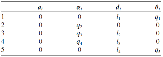
The feller buncher machine is modeled after the Tigercat 855E, and its kinematics can be described with the schematic diagram in Fig. 2 and the Denavit-Hartenberg parameters in Table II. The machine is considered to be holding onto a tree in the manipulation planning example, and the length
 $l_i$
and mass
$l_i$
and mass
 $m_i$
of each of the machine’s links and the tree are summarized in Table I. The machine’s support polygon is a
$m_i$
of each of the machine’s links and the tree are summarized in Table I. The machine’s support polygon is a
 $3.23\;\text{m }\!\!\!\times 5\;\text{m}$
rectangle.
$3.23\;\text{m }\!\!\!\times 5\;\text{m}$
rectangle.
Table I. Mobile manipulator parameters for the test case.

Table II. Denavit-Hartenberg parameters table of the feller buncher manipulator.
The optimal control results in this Section are achieved by running the general optimal control solver GPOPS [Reference Patterson and Rao47] under MATLAB environment on a Windows desktop with Intel Core i7-4770 3.40 GHz processor. The solver formulates a NOCP, through direct method, into a nonlinear programming problem. Despite the theoretical advantage of indirect method, due to the non-convexity of the ZMP inequality constraint, the necessary optimality condition is impossible to find without a priori knowledge on constraint occurrence [Reference Betts41]. Hence, direct method is chosen to solve problem (4) based on a quasi-static path.
Since the simplified manipulator model has
 $2$
arm DoFs while the full model has
$2$
arm DoFs while the full model has
 $5$
arm DoFs, to ensure that the ZMP location of the full model follows that of the simplified model, a relationship between the DoFs of the simplified model and those of the full model of the machine needs to be established. To satisfy Assumption 1(b), for the specific machine geometry in this example, we choose to constrain the machine’s joint angles such that
$5$
arm DoFs, to ensure that the ZMP location of the full model follows that of the simplified model, a relationship between the DoFs of the simplified model and those of the full model of the machine needs to be established. To satisfy Assumption 1(b), for the specific machine geometry in this example, we choose to constrain the machine’s joint angles such that
 \begin{equation} [q_3, q_4,q_5]^T = [\!-\!\pi -\!2q_2, \dfrac{\pi }{2}+q_2, \text{constant}]^T, \end{equation}
and the corresponding relationship between joint accelerations follows:
 \begin{equation} [\ddot{q}_3,\ddot{q}_4,\ddot{q}_5]^T = [\!-\!2\ddot{q}_2, \ddot{q}_2,0]^T. \end{equation}
The relationship between
 $d$
and
$d$
and
 $q_2$
can be written as:
$q_2$
can be written as:
 \begin{equation} q_2=\sin ^{-1}\left(\frac{-d}{2l_2}\right). \end{equation}
Then, taking the first and second derivative of (25) with respect to time, we can obtain:
 \begin{equation} \begin{aligned} \dot{q}_2 & = \dfrac{-\dot{d}}{2l_2\sqrt{1-\dfrac{d^2}{4l_2^2}}}\\[5pt] \ddot{q}_2 & = -\dfrac{\ddot{d}}{2l_2\sqrt{1-\dfrac{d^2}{4l_2^2}}}-\dfrac{d\dot{d}^2}{8l_2^3\sqrt{1-\dfrac{d^2}{4l_2^2}}^3}. \end{aligned} \end{equation}
Therefore, using the mapping provided in (23) and (24), and the relation between joint angles and accelerations as given in (25) and (26), the ZMP location of the full kinematics model can be written as
 $ \textbf{p}_{\text{zmp}}(\tilde{\textbf{x}},\tilde{\textbf{u}})$
.
$ \textbf{p}_{\text{zmp}}(\tilde{\textbf{x}},\tilde{\textbf{u}})$
.
5.2. Full kinematics vs. simplified formulation vs. phase plane method
In the first test case, we consider the feller buncher to be situated statically on a slope that results in a 30-degree vehicle roll to the left. The machine starts from this initial condition and the goal is to have the cabin yaw 180 degrees towards left. The initial joint angles and velocities are:
 \begin{equation} \begin{aligned} \textbf{q}(t_0) &= [0, -\pi/6, -2\pi/3, \pi/6, -\pi/2]^T \text{ rad}\\[5pt] \dot{\textbf{q}}(t_0) &= [0,0,0,0,0]^T \text{ rad/s}, \end{aligned} \end{equation}
and the desired final joint angles and velocities are:
 \begin{equation} \begin{aligned} \textbf{q}(t_f) &= [\pi, -\pi/6, -2\pi/3, \pi/6, -\pi/2]^T \text{ rad}\\[5pt] \dot{\textbf{q}}(t_f) &= [0,0,0,0,0]^T \text{ rad/s}. \end{aligned} \end{equation}
The joint rate and acceleration constraints are:
 \begin{align*} -\frac{\pi }{4} &\leq \dot{q}_i \leq \frac{\pi }{4} \text{ rad/s}\;\;\;\;\;\forall \; i\\[5pt] -\frac{\pi }{2} &\leq \ddot{q}_i \leq \frac{\pi }{2} \text{ rad/s}^2\;\;\;\;\forall \; i. \end{align*}
The ZMP loci of motions generated using the optimal trajectory planning formulation (4) with full kinematics model, the simplified kinematics model, and the classic phase plane method that considers joint angle, rate, and acceleration limits without stability constraints [Reference Shin and McKay25] are presented in Fig. 6. These results show that if the feller buncher follows the time-optimal trajectory prescribed by the phase plane method, the ZMP locus (green) of the machine will travel outside of the support polygon. In this case, the machine is at risk of rolling over. However, the motion generated through solving (4) with full kinematics model and the simplified kinematics model would result in safe (red and blue) ZMP loci. It is noted that although the starting and ending states of the machine for the three trajectory planning methods are the same, the ZMP loci do not start and end at the same points due to different initial accelerations. Additionally, even though the ZMP locus generated from the simplified model (blue) displays chattering behavior, the corresponding joint accelerations shown in Fig. 7(a) are sufficiently smooth. The unsafe motion generated by the phase plane method takes 4.5 s to complete; the safe motion generated by solving the NOCP (4) also takes 4.5 s to complete; and the safe motion generated with the simplified kinematics model takes 5.0 s to complete.

Figure 6. ZMP loci of constrained trajectory planning vs. phase plane method.

Figure 7. Joint accelerations (a), velocities (b), and angles (c) plots. Blue line indicates results from the simplified model, red line indicates results from the full model, black dashed lines indicate constraints. Note that all blue values of
 $q_5$
are zero due to this DoF being reduced in the simplified model.
$q_5$
are zero due to this DoF being reduced in the simplified model.
For the solutions of (4) and (4) with simplified kinematics, the planned joint accelerations, rates, and angles are displayed in Fig. 7(a), (b), and (c), respectively. It is noted that all initial and final conditions, and state and input constraints are satisfied for both the full and simplified formulations. However, for this example, the computation time to solve (4) is more than 5 h, while the computation time to solve with simplified kinematics is 1.34 s.
5.3. Monte Carlo simulations for reconfiguration on different slopes
To test the performance of the simplified model for different initial and final conditions, additional simulations were carried out for four different machine base attitudes of 0,15, 20, and 30-degree roll, each with 3000 pairs of randomized initial and final cabin yaw angles from the set
 $[\!-\!2\pi,2\pi ]$
with other initial and final joint angles the same as in (27) and (28). The trajectory planning success rate is presented in Table III. The distribution of successful trajectory planning times for the four base attitudes is presented in Fig. 8.
$[\!-\!2\pi,2\pi ]$
with other initial and final joint angles the same as in (27) and (28). The trajectory planning success rate is presented in Table III. The distribution of successful trajectory planning times for the four base attitudes is presented in Fig. 8.
It can be observed from these results that the planning success rate decreases with increasing slope angle, and computation time increases with increasing slope angle. The decreasing trend in success rate is due to the more frequent appearance of infeasible initial and final conditions. The distribution in Fig. 8 shows that the dimension reduction applied in the simplified model allows the computation time to be low enough for online guidance in most cases.
5.4. Mobile relocation planning
To test the performance of mobile relocation trajectory planning of Section 4, a test terrain described by the sinusoidal function:
 \begin{equation} s_z=10\cos \left(\frac{\sqrt{{s_x}^2+{s_y}^2}}{10}\right) \end{equation}
is created. To formulate the NOCP (4) of this example, the terrain surface function (29) is integrated into the feller buncher’s simplified kinematics (5). It is also noted that the simplified kinematics will be used for the remainder of the simulation results.
Table III. Trajectory planning success rate with simplified kinematics model for four base attitudes.


Figure 8. Computation time for reconfiguration maneuver of four slope angles using simplified model.

Figure 9. Planned path and point of reconfiguration of the feller buncher machine on a sinusoidal test terrain.
The machine itself, without the tree, is then commanded to start from the peak of a mountain (
 $s_x = 0$
,
$s_x = 0$
,
 $s_y = 0$
,
$s_y = 0$
,
 $s_z = 10$
) and to relocate to a point (
$s_z = 10$
) and to relocate to a point (
 $s_x = 0$
,
$s_x = 0$
,
 $s_y = 63$
,
$s_y = 63$
,
 $s_z \approx 10$
) on the surrounding ridge (see Fig. 9). Denoting the base’s linear velocity as
$s_z \approx 10$
) on the surrounding ridge (see Fig. 9). Denoting the base’s linear velocity as
 $v$
, the initial and final states for the machine’s base and arm are:
$v$
, the initial and final states for the machine’s base and arm are:
 \begin{equation*} \begin {aligned} [x_0,y_0,v,\bar \psi,\dot {\bar {\psi }}]^T(t_0)&=[0,0,0,0,0]^T\\[2pt] \textbf{q}(t_0) &= [0, -\pi/6, -2\pi/3, \pi/6, -\pi/2]^T\\[2pt] \dot {\textbf{q}}(t_0) &=[0,0,0,0,0]^T\\[2pt] [x_0,y_0,v,\bar \psi,\dot {\bar {\psi }}]^T(t_f)&=[0,63,0,\text {free},0]^T\\[2pt] \dot {\textbf{q}}(t_f) &=[0,0,0,0,0]^T, \end {aligned} \end{equation*}
and we note that the final heading angle of the base and arm joint angles are left free. The constraints on the mobile base’s linear and angular rates and accelerations are:
 \begin{equation*} \begin {aligned} 0\leq &v\leq 2.78\;\;\text {m}/\text {s}\\[5pt] -1\leq &u_a\leq 1\;\;\text {m}/\text {s}^2\\[5pt] -2\leq &\dot {\psi }\leq 2\;\;\text {rad}/\text {s}\\[5pt] -\frac {2}{3}\leq &u_{\psi }\leq \frac {2}{3}\;\;\text {rad}/\text {s}^2. \end {aligned} \end{equation*}
Algorithm 1 first generates a quasi-static path with guaranteed stability for continuous motion for the machine indicated by the blue crosses in Fig. 9. The run time for path generation is
 $2.00$
s. The resulting path requires the machine to reconfigure its cabin angle
$2.00$
s. The resulting path requires the machine to reconfigure its cabin angle
 $q_1$
, as shown by Fig. 9(a) and (b), to shift the ZMP so the machine does not rollover towards the front as it is descending the slope. The sampling point (sampling point #13) where this configuration change happens is highlighted in Fig. 9(c) by a red circle.
$q_1$
, as shown by Fig. 9(a) and (b), to shift the ZMP so the machine does not rollover towards the front as it is descending the slope. The sampling point (sampling point #13) where this configuration change happens is highlighted in Fig. 9(c) by a red circle.
Then, based on the quasi-static path and configuration change generated by Algorithm 1, an initial guess is given to the NOCP solver to generate linear and angular accelerations for the machine to allow for time-optimal relocation. The solver generates the trajectory of each segment with the initial and final location of a segment being two consecutive sampling points. To create an initial guess of each segment for the NOCP solver, the machine is constrained to be static at each sampling point but is given small constant linear velocity and heading rate to satisfy the quasi-static property. The resulting trajectories of all segments are then combined. The continuous path of the machine is represented by the red line in Fig. 9, the motion trajectory is shown in Fig. 10, and the ZMP trajectory is shown in Fig. 11. Note that the machine’s velocity remains 0 in segment 14 due to arm reconfiguration.

Figure 10. Motion trajectory generated by iteratively solving NOCP of each segment. Dashed vertical lines correspond to segments.

Figure 11. ZMP trajectory generated by iteratively solving NOCP of each segment.
The result in Fig. 10 shows that all state and stability constraint variables remained within their bounds, indicated by horizontal black dashed lines, and the overall trajectory takes
 $\approx 180$
s to complete. Each motion segment separated by vertical dashed lines took
$\approx 180$
s to complete. Each motion segment separated by vertical dashed lines took
 $\approx 0.30$
s to calculate, and the entire trajectory took
$\approx 0.30$
s to calculate, and the entire trajectory took
 $18.30$
s to plan. This shows that the framework proposed in this paper can be implemented to provide online stability-constrained trajectory planning.
$18.30$
s to plan. This shows that the framework proposed in this paper can be implemented to provide online stability-constrained trajectory planning.
The resulting ZMP trajectory is shown in Fig. 11 with black dashed horizontal lines indicating the boundaries of
 $Conv(S)$
. During sampling-based path planning, the deviation of
$Conv(S)$
. During sampling-based path planning, the deviation of
 $x_{zmp}$
from the centerline of
$x_{zmp}$
from the centerline of
 $Conv(S)$
is constrained to change linearly with respect to the slope angle from
$Conv(S)$
is constrained to change linearly with respect to the slope angle from
 $50\%$
of the total width of
$50\%$
of the total width of
 $Conv(S)$
on flat ground to
$Conv(S)$
on flat ground to
 $10\%$
on
$10\%$
on
 $45^o$
slopes. The machine’s
$45^o$
slopes. The machine’s
 $x_{zmp}$
is shown to have stayed close to
$x_{zmp}$
is shown to have stayed close to
 $0$
, that is, the centerline of the support polygon, during ascent and descent as a result of the traction-optimized path as mentioned in Section 4.4. The location of
$0$
, that is, the centerline of the support polygon, during ascent and descent as a result of the traction-optimized path as mentioned in Section 4.4. The location of
 $y_{zmp}$
is shown to generally move forward as the machine is moving down the slope and then move backward as the machine is climbing the slope. However, due to the quasi-static inter-segment constraint, the overall motion of the machine is not satisfactory: the velocities and accelerations are highly oscillatory (see the subfigures for
$y_{zmp}$
is shown to generally move forward as the machine is moving down the slope and then move backward as the machine is climbing the slope. However, due to the quasi-static inter-segment constraint, the overall motion of the machine is not satisfactory: the velocities and accelerations are highly oscillatory (see the subfigures for
 $a$
and
$a$
and
 $\ddot{\psi }$
) and can cause less than ideal performance, along with excessive hardware wear. To remedy this, a receding horizon NOCP solution scheme is implemented.
$\ddot{\psi }$
) and can cause less than ideal performance, along with excessive hardware wear. To remedy this, a receding horizon NOCP solution scheme is implemented.
For the result shown in Fig. 10, more than one trajectory segment can be treated as a whole and thus used as the initial guess of a new NOCP segment. The length of time interval in the new combined segment will be called “horizon length.” For this specific example, the horizon length is chosen to be
 $\approx 4$
s. For each segment, when the solver cannot converge to a solution within a user specified time threshold, the re-planning is considered “unsuccessful,” and the solver is terminated for the current segment and the re-planning carries on to the next segment. When a re-planning is unsuccessful, the iterative result computed for the original segment is kept. This way, the motion trajectory can be optimized where possible to reduce the occurrence of machine stop-and-go.
$\approx 4$
s. For each segment, when the solver cannot converge to a solution within a user specified time threshold, the re-planning is considered “unsuccessful,” and the solver is terminated for the current segment and the re-planning carries on to the next segment. When a re-planning is unsuccessful, the iterative result computed for the original segment is kept. This way, the motion trajectory can be optimized where possible to reduce the occurrence of machine stop-and-go.
The receding horizon scheme enhanced motion trajectory is shown in Fig. 12, with the corresponding ZMP trajectory shown in Fig. 13. It can be observed that, compared to Fig. 10, the motion trajectory has become significantly smoother. The relocation completion time has also been shortened to
 $\approx 93$
s due to the enhancement. Both the state and dynamic stability constraints are shown to be respected. The joint motion trajectories of the arm are shown in Fig. 14. The joint variables vary only in one segment which corresponds to 0 velocity of the machine’s base, when the robot reconfigures itself. The successful receding horizon re-planning segments took a total
$\approx 93$
s due to the enhancement. Both the state and dynamic stability constraints are shown to be respected. The joint motion trajectories of the arm are shown in Fig. 14. The joint variables vary only in one segment which corresponds to 0 velocity of the machine’s base, when the robot reconfigures itself. The successful receding horizon re-planning segments took a total
 $10.52$
s to complete, while the 20 unsuccessful segments took a total of
$10.52$
s to complete, while the 20 unsuccessful segments took a total of
 $10.00$
s with the computational time threshold set to
$10.00$
s with the computational time threshold set to
 $0.5$
s. The time-optimal trajectories exhibit behaviors similar to bang-bang control except when ZMP constraint violations are imminent.
$0.5$
s. The time-optimal trajectories exhibit behaviors similar to bang-bang control except when ZMP constraint violations are imminent.

Figure 12. Motion trajectory generated through iteratively solving NOCP with existing motion trajectory and a horizon length of 20 time steps.

Figure 13. ZMP trajectory generated through iteratively solving NOCP with existing motion trajectory and a horizon length of 20 time steps.

Figure 14. Joint motion trajectories of the machine with joint angles shown in red and joint velocities shown in blue.
5.5. Comparison to existing methods
As discussed in Section 1.2 and to the best of the authors knowledge, there are no existing methods to address the time-optimal, dynamic-stability-constrained, point-to-point trajectory planning of a mobile robot on 3D rough terrain. Hence, comparison to the state of the art presented here is carried out in a more general context, by comparing the hierarchical framework solution proposed in this paper to other general methods used in mobile robot motion planning. Since as noted in Section 1.2, the sampling-based planning methods are generally used for geometric planning only, because of their exponential growth in computation time with planning dimension, NOCP-based methods are considered for our comparison.
5.5.1. Qualitative comparison with NOCP method
Taking [Reference Rasekhipour, Khajepour, Chen and Litkouhi48] as an example, the NOCP-based planners typically employ a PF to formulate the NOCP to drive the robot towards its goal while avoiding obstacles. Then, Sequential Quadratic Programming (SQP) [Reference Boggs and Tolle49] is applied to solve the NOCP in a timely manner. However, applying a PF-based NOCP formulation with an SQP solver to our problem statement in (4) will pose two major difficulties: One, the terrain map is non-convex, and the ZMP constraint is non-convex with respect to the robot’s state and control input. It is well-known that a PF-based formulation in the presence of non-convex constraints will trap the solution in a local minimum [Reference Liu, Ang, Krishnan and Yong50]. Although a number of previous papers presented work-arounds to this local minimum issue in the context of static obstacle avoidance, a work-around that deals with an acceleration input and velocity-dependent constraints has yet to be put forward. Two, the time-optimal aspect of (4) results in difficulties in the SQP formulation. As demonstrated in [Reference Verschueren, van Duijkeren, Swevers and Diehl28], the kinematics of a robot in a time-optimal robotic planning problem has to be parametrized by a path parameter for the NOCP to be solved efficiently by SQP, which means a pre-determined geometric path that is feasible is required.
With the above considerations, in the following, the merit of the proposed method will be demonstrated by comparing our solution to that of a popular alternative where a MPC scheme is used to guide a robot along an existing ZMP-stable path. Here, MPC is chosen due to its popularity in trajectory tracking applications and its computational efficiency [Reference He, Wang and Song51].
5.5.2. Model predictive control path following
To highlight the importance of enforcing the dynamic stability constraint during the trajectory generation stage, the trajectory generated with the proposed framework is compared to the motion obtained with MPC. Since path generation is not of interest in this comparison, the same quasi-static ZMP-stable path will be used. The path considered traverses through a sub-area of the test terrain employed in Section 5.4, (defined with (29)) and is formed by waypoints generated using RRT
 $\mathcal{S}$
(Algorithm 1). For easier comparison, the path is generated without considering manipulator configuration change, nor traction optimization.
$\mathcal{S}$
(Algorithm 1). For easier comparison, the path is generated without considering manipulator configuration change, nor traction optimization.
In this comparison, the MPC controller is employed to drive a linearized unicycle model along a reference trajectory on the test terrain optimally, by iteratively minimizing the quadratic tracking error, within a finite time horizon. A reference trajectory along the path will be generated by assigning uniform path velocities. A detailed explanation of the formulation and implementation of MPC that we follow can be found in ref. [Reference Rawlings52]. Even though MPC cannot easily accommodate the nonlinear ZMP constraint and the time optimality formulation, the purpose of MPC is nonetheless similar to the NOCP portion of our hierarchical framework in that they both aim to generate locally optimal trajectories based on an existing path. It is worth pointing out that even though NMPC (Nonlinear MPC) has the ability to accommodate the ZMP stability and time-optimization aspects by employing (4) in its formulation, it is treated as a finite-horizon special case of (4) in this paper as it still requires the controlled invariant set proof of Theorem 4.1 and other techniques from this work to perform efficiently and reliably.
5.5.3. Quantitative comparison results with MPC
For the implementation of MPC, we set the sampling period to
 $0.2$
s, prediction horizon to
$0.2$
s, prediction horizon to
 $5$
steps, and control horizon to
$5$
steps, and control horizon to
 $2$
steps. Further details on the setup, parameters, and performance of the MPC scheme can be found in Appendix C. Two MPC examples are provided in this comparison: for the first, referred to as “RRT
$2$
steps. Further details on the setup, parameters, and performance of the MPC scheme can be found in Appendix C. Two MPC examples are provided in this comparison: for the first, referred to as “RRT
 $\mathcal{S}$
+MPC (slow),” the reference input to MPC is a constant velocity of
$\mathcal{S}$
+MPC (slow),” the reference input to MPC is a constant velocity of
 $0.1$
m/s, while for the second, named “RRT
$0.1$
m/s, while for the second, named “RRT
 $\mathcal{S}$
+MPC (fast),” the reference is a higher constant velocity of
$\mathcal{S}$
+MPC (fast),” the reference is a higher constant velocity of
 $1$
m/s. The resulting paths and velocity profiles are shown in Fig. 15(a) and (b), respectively. In these plots, the color map represents the velocity profile ranging from
$1$
m/s. The resulting paths and velocity profiles are shown in Fig. 15(a) and (b), respectively. In these plots, the color map represents the velocity profile ranging from
 $0$
m/s to
$0$
m/s to
 $1.6$
m/s as the corresponding color turns from cold (blue) to warm (yellow). The corresponding ZMP trajectories resulting from the two MPC trajectories are shown in Fig. 15(c) where the horizontal (time) axis has been normalized for ease of comparison. The trajectories take
$1.6$
m/s as the corresponding color turns from cold (blue) to warm (yellow). The corresponding ZMP trajectories resulting from the two MPC trajectories are shown in Fig. 15(c) where the horizontal (time) axis has been normalized for ease of comparison. The trajectories take
 $180$
s and
$180$
s and
 $21$
s to complete, for the slow and fast examples, respectively. It can be observed that even though “RRT
$21$
s to complete, for the slow and fast examples, respectively. It can be observed that even though “RRT
 $\mathcal{S}$
+MPC (fast)” took significantly less time to reach the goal point, it resulted in large ZMP constraint violation near
$\mathcal{S}$
+MPC (fast)” took significantly less time to reach the goal point, it resulted in large ZMP constraint violation near
 $0.6$
time unit. On the path shown in Fig. 15(b), this ZMP constraint violation corresponds to the second turn where the machine is commanded to retain higher velocity compared to “RRT
$0.6$
time unit. On the path shown in Fig. 15(b), this ZMP constraint violation corresponds to the second turn where the machine is commanded to retain higher velocity compared to “RRT
 $\mathcal{S}$
+MPC (slow)” and “Proposed” before exiting the turn. This is a direct result of the controller only following a quasi-statically ZMP-stable path, without taking the dynamic ZMP stability into consideration.
$\mathcal{S}$
+MPC (slow)” and “Proposed” before exiting the turn. This is a direct result of the controller only following a quasi-statically ZMP-stable path, without taking the dynamic ZMP stability into consideration.

Figure 15. Comparison between MPC path tracking results with slow and fast uniform velocity reference trajectories and the trajectory generated using the proposed framework.
Following the proposed framework, the path generated with Algorithm 1 is treated as a quasi-static trajectory with a low velocity of
 $0.1$
m/s to warm start (4). The computation time to generate the iterative solution for all
$0.1$
m/s to warm start (4). The computation time to generate the iterative solution for all
 $15$
segments is
$15$
segments is
 $4.62$
s, and the receding horizon re-planning then takes a total of
$4.62$
s, and the receding horizon re-planning then takes a total of
 $5.67$
s with
$5.67$
s with
 $8$
unsuccessful segments’ computational time going over the threshold of
$8$
unsuccessful segments’ computational time going over the threshold of
 $0.5$
s. The average time to initially plan a segment is
$0.5$
s. The average time to initially plan a segment is
 $0.31$
s, and the average successful re-planning time for each segment is
$0.31$
s, and the average successful re-planning time for each segment is
 $0.24$
. The planned trajectory of each segment takes an average of
$0.24$
. The planned trajectory of each segment takes an average of
 $1.7$
s to complete. The final trajectory takes
$1.7$
s to complete. The final trajectory takes
 $24$
s to complete, and the final path is plotted in Fig. 15(b), for direct comparison to “RRT
$24$
s to complete, and the final path is plotted in Fig. 15(b), for direct comparison to “RRT
 $\mathcal{S}$
+MPC (fast)” solution. Figure 15(b) shows that the velocity profile for the “Proposed” solution trajectory decreased to a lower value, as compared to “RRT
$\mathcal{S}$
+MPC (fast)” solution. Figure 15(b) shows that the velocity profile for the “Proposed” solution trajectory decreased to a lower value, as compared to “RRT
 $\mathcal{S}$
+MPC (fast),” before reaching the apex of the second turn. The ZMP trajectory corresponding to the proposed framework solution remains within the support polygon for the whole maneuver (see Fig. 15(c)).
$\mathcal{S}$
+MPC (fast),” before reaching the apex of the second turn. The ZMP trajectory corresponding to the proposed framework solution remains within the support polygon for the whole maneuver (see Fig. 15(c)).
The comparison presented here clearly demonstrates that the dynamic stability constraint has to be respected in both path and trajectory generation for safe and time-efficient robot motion. The proposed hierarchical solution framework can directly accomplish this goal. Although the reference trajectory for MPC can be tuned through trial and error to have a sufficiently slow velocity to approach the quasi-static ZMP-stable conditions, this can drastically reduce the motion efficiency.
6. Conclusions and future work
To conclude, this paper presented a framework that allows online time-optimal point-to-point mobile manipulation trajectory planning to provide motion guidance for a robot to work safely and efficiently on rough terrain. This is achieved through the formulation of a trajectory planning problem as an optimal control problem with an additional dynamic stability constraint. To reduce the problem dimension, the mobile manipulation task is first divided into two separate stages: the manipulation stage and the relocation stage. The online trajectory planning of the manipulation stage is achieved through dimension reduction with the help of the known inverse kinematics mapping of the robot. Then, to solve the relocation planning problem, a sampling-based planning algorithm that optimizes slope traction availability and generates results guaranteed to meet non-convex stability constraints when continuously executed is implemented. The robot path and reconfiguration command generated by the sampling-based algorithm are then taken to warm start a NOCP solver. The resulting trajectory is further optimized and smoothed with the receding horizon re-planning scheme. Both qualitative and quantitative simulation comparisons to other popular approaches are presented to showcase the benefit of the proposed framework.
The framework presented in this paper is the first attempt at a task-based online optimal planning algorithm for a mobile manipulator that accommodates the nonlinear dynamic stability constraint. Some further work can be done for the framework to be implemented in a wider variety of scenarios. For example, the terrain map used in this paper only assumes a rough knowledge of the terrain features. However, as the robot traverses through the terrain, more detailed terrain features can be captured by its on-board sensors. With a more detailed local terrain map, a re-planning method or a stability-guaranteed control law can be developed to help the robot deal with local terrain complexities.
Conflicts of interest
None.
Financial support and acknowledgement
This work was supported by the National Sciences and Engineering Research Council (NSERC) Canadian Robotics Network (NCRN), the McGill Engineering Doctoral Awards and Summer Undergraduate Research in Engineering (SURE) programs. The authors would also like to thank Centre de Formation Professionnelle Mont-Laurier for their help during field work.
Ethical considerations
None.
Authors’ contributions
Both authors conceived and designed the study, and wrote the article. J. Song conducted analysis and data gathering.
A. Proof of Theorem 4.1
Proof 2. A mobile robot with unicycle kinematics follows a quasi-static path with two motion primitives: forward and turn. We define any state or ZMP constraint variable
 $(\cdot )$
found under static condition:
$(\cdot )$
found under static condition:
 $[\dot{\textbf{x}}^T,\textbf{u}^T]^T=\textbf{0}$
as a static variable denoted by
$[\dot{\textbf{x}}^T,\textbf{u}^T]^T=\textbf{0}$
as a static variable denoted by
 $(\cdot )^{\text{static}}$
. Its dynamic counterpart, denoted by
$(\cdot )^{\text{static}}$
. Its dynamic counterpart, denoted by
 $(\cdot )^{\text{dynamic}}$
, is found with any feasible
$(\cdot )^{\text{dynamic}}$
, is found with any feasible
 $[\dot{\textbf{x}}^T,\textbf{u}^T]^T$
. The Euclidean distance between
$[\dot{\textbf{x}}^T,\textbf{u}^T]^T$
. The Euclidean distance between
 $\textbf{p}_{zmp}^{\text{dynamic}}$
and
$\textbf{p}_{zmp}^{\text{dynamic}}$
and
 $\textbf{p}_{zmp}^{\text{static}}$
can be characterized using the 2-norm:
$\textbf{p}_{zmp}^{\text{static}}$
can be characterized using the 2-norm:
 $||\textbf{p}_{zmp}^{\text{dynamic}}-\textbf{p}_{zmp}^{\text{static}}||_2$
. Here,
$||\textbf{p}_{zmp}^{\text{dynamic}}-\textbf{p}_{zmp}^{\text{static}}||_2$
. Here,
 $\textbf{p}_{zmp}^{\text{dynamic}}$
and
$\textbf{p}_{zmp}^{\text{dynamic}}$
and
 $\textbf{p}_{zmp}^{\text{static}}$
can both be found from (3).
$\textbf{p}_{zmp}^{\text{static}}$
can both be found from (3).
Under the assumption that straight line segments connecting the nodes are short so that the robot’s attitude change during forward motion is negligible, we have
 $\ddot{x}_i^{\text{dynamic}}=\ddot{x}_i^{\text{static}}=0$
, and
$\ddot{x}_i^{\text{dynamic}}=\ddot{x}_i^{\text{static}}=0$
, and
 $\ddot{z}_i^{\text{dynamic}}=\ddot{z}_i^{\text{static}}=0$
 $\forall i\in \{0,\cdots,n\}$
. Therefore,
$\forall i\in \{0,\cdots,n\}$
. Therefore,
 $x_{zmp}^{\text{dynamic}}=x_{zmp}^{\text{static}}$
. As a result, we obtain the following during forward motion:
$x_{zmp}^{\text{dynamic}}=x_{zmp}^{\text{static}}$
. As a result, we obtain the following during forward motion:
 \begin{equation} \begin{aligned} \left |\left |\textbf{p}_{zmp}^{\text{dynamic}}-\textbf{p}_{zmp}^{\text{static}}\right |\right |_2 &=\left |y_{zmp}^{\text{dynamic}}-y_{zmp}^{\text{static}}\right |\\[5pt] &=\left |\frac{\sum _im_i \ddot{y}_i^{\text{dynamic}}z_i}{\sum _im_ig_z}\right |\\[5pt] &\leq \left |\frac{\sum _im_i z_i}{\sum _im_ig_z}\right |\left |\ddot{y}^{\text{dynamic}}\right |\\[5pt] &=\left |\frac{\sum _im_i z_i}{\sum _im_ig_z}\right |\left |u_a\right |. \end{aligned} \end{equation}
Derivation in (30) shows that, the distance between
 $\textbf{p}_{zmp}^{\text{static}}$
and
$\textbf{p}_{zmp}^{\text{static}}$
and
 $\textbf{p}_{zmp}^{\text{dynamic}}$
during forward motion is proportionally bounded by the magnitude of input
$\textbf{p}_{zmp}^{\text{dynamic}}$
during forward motion is proportionally bounded by the magnitude of input
 $u_a$
and is independent of velocity
$u_a$
and is independent of velocity
 $v$
. Hence, there exists input
$v$
. Hence, there exists input
 $u_a(t)$
 $\forall \;t\in [t_0,t_f]$
, such that
$\forall \;t\in [t_0,t_f]$
, such that
 $v\gt 0$
and
$v\gt 0$
and
 $\left |\left |\textbf{p}_{zmp}^{\text{dynamic}}\!\!-\!\!\textbf{p}_{zmp}^{\text{static}}\right |\right |_2 \leq \sigma$
for arbitrarily small
$\left |\left |\textbf{p}_{zmp}^{\text{dynamic}}\!\!-\!\!\textbf{p}_{zmp}^{\text{static}}\right |\right |_2 \leq \sigma$
for arbitrarily small
 $\sigma \gt 0$
on straight line segments.
$\sigma \gt 0$
on straight line segments.
For the unicycle turning motion, every link on the robot goes through a rotation about the
 $z_0$
-axis that can be described by the following rotation matrix:
$z_0$
-axis that can be described by the following rotation matrix:
 \begin{equation} R_{yaw}=\begin{bmatrix} \cos{\psi }&-\!\sin{\psi }&0\\[5pt] \sin{\psi }&\cos{\psi }&0\\[5pt] 0&0&1 \end{bmatrix}. \end{equation}
With the mobile base location fixed during the turn, the linear acceleration of each link’s center of mass can be written as:
 \begin{equation} \begin{bmatrix} \ddot{x}_i\\[5pt] \ddot{y}_i\\[5pt] \ddot{z}_i \end{bmatrix} =\underbrace{ \begin{bmatrix} -\!\cos{\psi }\dot{\psi }^2 - \sin{\psi }u_{\psi } & \sin{\psi }\dot{\psi }^2 - \cos{\psi }u_{\psi }&0\\[5pt] - \!\sin{\psi }\dot{\psi }^2 + \cos{\psi }u_{\psi } & - \cos{\psi }\dot{\psi }^2 - \sin{\psi }u_{\psi }&0\\[5pt] 0&0&0 \end{bmatrix} }_{\ddot{R}_{yaw}} \begin{bmatrix} x_i\\[5pt] y_i\\[5pt] z_i \end{bmatrix}. \end{equation}
Then, the distance between dynamic and static ZMPs during turning motion can be written as:
 \begin{equation} \begin{aligned} &\;\;\left |\left |\textbf{p}_{zmp}^{\text{dynamic}}\!\!-\!\!\textbf{p}_{zmp}^{\text{static}}\right |\right |_2\\[5pt] &= \left |\left |\left [x_{zmp}^{\text{dynamic}}-x_{zmp}^{\text{static}},y_{zmp}^{\text{dynamic}}-y_{zmp}^{\text{static}}\right ]^T\right |\right |_2=\left |\left |\left [\frac{\sum _i m_i\ddot{x}_i^{\text{dynamic}}\!z_i}{\sum _im_ig_z},\frac{\sum _im_i\ddot{y}_i^{\text{dynamic}}z_i}{\sum _im_ig_z} \right ]^T\right |\right |_2\\[5pt] &\leq \left |\frac{\sum _i m_i\ddot{x}_i^{\text{dynamic}}\!z_i}{Mg_z}\right |+\left |\frac{\sum _i m_i\ddot{y}_i^{\text{dynamic}}\!z_i}{Mg_z}\right |\\[5pt] &=\left |\left [\frac{m_0z_0}{Mg_z},\cdots,\frac{m_nz_n}{Mg_z}\right ]\left [\ddot{x}_0^{\text{dynamic}},\cdots,\ddot{x}_n^{\text{dynamic}} \right ]^T \right |+\left |\left [\frac{m_0z_0}{Mg_z},\cdots,\frac{m_nz_n}{Mg_z}\right ]\left [\ddot{y}_0^{\text{dynamic}},\cdots,\ddot{y}_n^{\text{dynamic}} \right ]^T \right |\\[5pt] &\leq \left |\left |\left [\frac{m_0z_0}{Mg_z},\cdots,\frac{m_nz_n}{Mg_z}\right ]\right |\right |_2 \bigg (\left |\left |\left [\ddot{x}_0^{\text{dynamic}},\cdots,\ddot{x}_n^{\text{dynamic}} \right ]\right |\right |_2+\left |\left |\left [\ddot{y}_0^{\text{dynamic}},\cdots,\ddot{y}_n^{\text{dynamic}} \right ]\right |\right |_2\bigg )\\[5pt] &\leq 2\left |\left |\left [\frac{m_0z_0}{Mg_z},\cdots,\frac{m_nz_n}{Mg_z}\right ]\right |\right |_2 \sum _i(|x_i|\dot{\psi }^2+|x_i||u_{\psi }|+|y_i|\dot{\psi }^2+|y_i||u_{\psi }|)\\[5pt] &=2\left |\left |\left [\frac{m_0z_0}{Mg_z},\cdots,\frac{m_nz_n}{Mg_z}\right ]\right |\right |_2 \sum _i\left (|x_i|+|y_i|\right )(\dot{\psi }^2+|u_{\psi }|) \end{aligned} \end{equation}
Inequality (33) shows that the distance between
 $\textbf{p}_{zmp}^{\text{static}}$
and
$\textbf{p}_{zmp}^{\text{static}}$
and
 $\textbf{p}_{zmp}^{\text{dynamic}}$
during turning motion is proportionally bounded by
$\textbf{p}_{zmp}^{\text{dynamic}}$
during turning motion is proportionally bounded by
 $(\dot{\psi }^2+|u_{\psi }|)$
. Then, it can be inferred that there exists a positive value
$(\dot{\psi }^2+|u_{\psi }|)$
. Then, it can be inferred that there exists a positive value
 $\epsilon$
such that
$\epsilon$
such that
 $\left |\left |\textbf{p}_{zmp}^{\text{dynamic}}\!\!-\!\!\textbf{p}_{zmp}^{\text{static}}\right |\right |_2 \leq \sigma$
for an arbitrarily small
$\left |\left |\textbf{p}_{zmp}^{\text{dynamic}}\!\!-\!\!\textbf{p}_{zmp}^{\text{static}}\right |\right |_2 \leq \sigma$
for an arbitrarily small
 $\sigma \gt 0$
during turning motion as long as
$\sigma \gt 0$
during turning motion as long as
 $(\dot{\psi }^2+|u_{\psi }|)\leq \epsilon$
. It is further claimed that, there exists
$(\dot{\psi }^2+|u_{\psi }|)\leq \epsilon$
. It is further claimed that, there exists
 $\dot{\psi }(t)$
and
$\dot{\psi }(t)$
and
 $u_{\psi }(t)$
pair
$u_{\psi }(t)$
pair
 $\forall \;t\in [t_0,t_f]$
, such that
$\forall \;t\in [t_0,t_f]$
, such that
 $\text{sign}(\dot{\psi })=\text{sign}(\psi )$
,
$\text{sign}(\dot{\psi })=\text{sign}(\psi )$
,
 $(\dot{\psi }^2+|u_{\psi }|)\leq \epsilon$
, and
$(\dot{\psi }^2+|u_{\psi }|)\leq \epsilon$
, and
 $\dot{\psi }(t)=\int u_{\psi }(t) dt$
.
$\dot{\psi }(t)=\int u_{\psi }(t) dt$
.
Hence, combining (30) and (33), there exists a trajectory
 $\textbf{u}(t)$
 $\forall \;t$
such that
$\forall \;t$
such that
 $\dot \tau \gt 0$
over the unit interval
$\dot \tau \gt 0$
over the unit interval
 $I$
, and
$I$
, and
 $\tau \to 1$
within finite time.
$\tau \to 1$
within finite time.
B. Proof of Proposition 2
Proof 3. To find the variation in ZMP location with respect to
 $\phi ^r$
and
$\phi ^r$
and
 $\theta ^r$
each, we take the corresponding partial derivatives of
$\theta ^r$
each, we take the corresponding partial derivatives of
 $G_1$
and
$G_1$
and
 $G_2$
. Furthermore, with the previously stated assumption that the distances between neighboring sampling points are small, we evaluate the partial derivatives at zero angles
$G_2$
. Furthermore, with the previously stated assumption that the distances between neighboring sampling points are small, we evaluate the partial derivatives at zero angles
 $\phi ^r\approx 0$
and
$\phi ^r\approx 0$
and
 $\theta ^r\approx 0$
, and obtain:
$\theta ^r\approx 0$
, and obtain:
 \begin{equation} \begin{aligned} \frac{\partial G_1}{\partial \phi ^r} &= -1-\frac{r_{13}^2}{r_{33}^2}\;\;\;\frac{\partial G_1}{\partial \theta ^r} = -\frac{r_{13}r_{23}}{r_{33}^2}\\[5pt] \frac{\partial G_2}{\partial \phi ^r} &= -\frac{r_{13}r_{23}}{r_{33}^2}\;\;\;\; \frac{\partial G_2}{\partial \theta ^r} = 1+\frac{r_{23}^2}{r_{33}^2}. \end{aligned} \end{equation}
Recalling the orthonormality of the rotation matrix so that
 $r_{13}^2+r_{23}^2+r_{33}^2=1$
, and that
$r_{13}^2+r_{23}^2+r_{33}^2=1$
, and that
 $r_{33}^2\geq r_{13}^2+r_{23}^2$
for ground robot operation on slopes under
$r_{33}^2\geq r_{13}^2+r_{23}^2$
for ground robot operation on slopes under
 $45$
degrees, the following can be inferred from (34):
$45$
degrees, the following can be inferred from (34):
 \begin{equation} \begin{aligned} \frac{\partial G_1}{\partial \phi ^r} &\leq -1,\;\;\frac{\partial G_1}{\partial \theta ^r} \approx 0\\[5pt] \frac{\partial G_2}{\partial \phi ^r} & \approx 0,\;\;\;\;\frac{\partial G_2}{\partial \theta ^r} \geq 1. \end{aligned} \end{equation}
By substituting (35) into (15), we obtain the following constraints on the variation of ZMP coordinates:
 \begin{equation} \begin{aligned} \frac{\partial x^r_{\text{zmp}}}{\partial{\phi ^r}} &\geq \frac{M_z}{M}\gt 0,\;\;\frac{\partial x^r_{\text{zmp}}}{\partial{\theta ^r}} \approx 0\\[5pt] \frac{\partial y^r_{\text{zmp}}}{\partial{\phi ^r}} &\approx 0,\;\;\;\;\;\;\;\;\;\;\;\frac{\partial y^r_{\text{zmp}}}{\partial{\theta ^r}} \leq -\frac{M_z}{M}\lt 0. \end{aligned} \end{equation}
C. Details of the MPC controller implementation
The discrete-time MPC controller is implemented using MATLAB’s Model Predictive Control Toolbox in Simulink. Since no arm reconfiguration is considered for this demonstration, the states of interest at time step
 $k$
can be defined as
$k$
can be defined as
 $\textbf{x}_{\text{MPC}}(k)=[x_{0,k},y_{0,k},v_k,\bar \psi _k,\dot{\bar{\psi }}_k]^T$
. For a time-stamped reference trajectory
$\textbf{x}_{\text{MPC}}(k)=[x_{0,k},y_{0,k},v_k,\bar \psi _k,\dot{\bar{\psi }}_k]^T$
. For a time-stamped reference trajectory
 $\textbf{x}^{\text{ref}}_{\text{MPC}}$
, tracking error at time step
$\textbf{x}^{\text{ref}}_{\text{MPC}}$
, tracking error at time step
 $k$
can be defined as
$k$
can be defined as
 $\textbf{e}(k)=\textbf{x}_{\text{MPC}}(k)-\textbf{x}^{\text{ref}}_{\text{MPC}}(k)$
. The machine is represented by a linearized unicycle model moving on 2-D coordinates:
$\textbf{e}(k)=\textbf{x}_{\text{MPC}}(k)-\textbf{x}^{\text{ref}}_{\text{MPC}}(k)$
. The machine is represented by a linearized unicycle model moving on 2-D coordinates:
 ${\textbf{x}}_{\text{MPC}}(k+1)=A\textbf{x}_{\text{MPC}}(k)+B\textbf{u}_{\text{MPC}}(k)$
, where control input at time step
${\textbf{x}}_{\text{MPC}}(k+1)=A\textbf{x}_{\text{MPC}}(k)+B\textbf{u}_{\text{MPC}}(k)$
, where control input at time step
 $k$
is denoted by
$k$
is denoted by
 $\textbf{u}_{\text{MPC}}(k)=[u_{a,k}, u_{\psi,k}]^T$
.
$\textbf{u}_{\text{MPC}}(k)=[u_{a,k}, u_{\psi,k}]^T$
.
The MPC is designed to minimize cost function
 $J_k=\sum _{i=0}^{p-1} \textbf{e}^T(k+i)Q\textbf{e}(k+i)$
subject to the linearized unicycle model with the same joint initial condition, state constraint, and input constraint as in Section 5.4. The positive semi-definite cost matrix is chosen to be
$J_k=\sum _{i=0}^{p-1} \textbf{e}^T(k+i)Q\textbf{e}(k+i)$
subject to the linearized unicycle model with the same joint initial condition, state constraint, and input constraint as in Section 5.4. The positive semi-definite cost matrix is chosen to be
 $Q=\text{diag}[1,1,0.1,1,0]$
to achieve position and heading angle tracking. No reference input tracking weight is included in cost function
$Q=\text{diag}[1,1,0.1,1,0]$
to achieve position and heading angle tracking. No reference input tracking weight is included in cost function
 $J_k$
. The cost history of both applications of MPC is shown in Fig. 16.
$J_k$
. The cost history of both applications of MPC is shown in Fig. 16.

Figure 16. Cost history of the MPC controller in “RRT
 $\mathcal{S}$
+MPC (slow)” and “RRT
$\mathcal{S}$
+MPC (slow)” and “RRT
 $\mathcal{S}$
+MPC (fast)”.
$\mathcal{S}$
+MPC (fast)”.


 Open access