


1 Introduction
The incorporation of kinetic effects, such as Landau damping, into a fluid description naturally requires some knowledge of kinetic theory. There are many excellent plasma physics books available, for example Akhiezer et al. (Reference Akhiezer, Akhiezer, Polovin, Sitenko and Stepanov1975), Swanson (Reference Swanson1989), Stix (Reference Stix1992), Gary (Reference Gary1993), Gurnett & Bhattacharjee (Reference Gurnett and Bhattacharjee2005), Fitzpatrick (Reference Fitzpatrick2015) and many others. These books cover numerous topics in kinetic theory that need to be addressed, if a plasma physics book wants to be considered complete. However, the topics that are required for the construction of advanced fluid models are often covered only briefly, or not covered at all. For example, the Padé approximation of the Maxwellian plasma dispersion function
 $Z(\unicode[STIX]{x1D701})$
or the plasma response function
$Z(\unicode[STIX]{x1D701})$
or the plasma response function
 $R(\unicode[STIX]{x1D701})=1+\unicode[STIX]{x1D701}Z(\unicode[STIX]{x1D701})$
, which is a crucial technique for the construction of collisionless fluid closures valid for all
$R(\unicode[STIX]{x1D701})=1+\unicode[STIX]{x1D701}Z(\unicode[STIX]{x1D701})$
, which is a crucial technique for the construction of collisionless fluid closures valid for all
 $\unicode[STIX]{x1D701}$
, is not addressed by any of the cited plasma books.
$\unicode[STIX]{x1D701}$
, is not addressed by any of the cited plasma books.
A researcher interested in collisionless fluid models that incorporate kinetic effects has to follow for example Hammett & Perkins (Reference Hammett and Perkins1990), Hammett, Dorland & Perkins (Reference Hammett, Dorland and Perkins1992), Snyder, Hammett & Dorland (Reference Snyder, Hammett and Dorland1997), Passot & Sulem (Reference Passot and Sulem2003), Goswami, Passot & Sulem (Reference Goswami, Passot and Sulem2005), Passot & Sulem (Reference Passot and Sulem2006, Reference Passot and Sulem2007), Passot, Sulem & Hunana (Reference Passot, Sulem and Hunana2012), Sulem & Passot (Reference Sulem and Passot2015) and references therein. The first three cited references are written in the guiding-centre reference frame (gyrofluid), which is a very powerful approach that enables the derivation of many results in an elegant way. However, the calculations in guiding-centre coordinates can be very difficult to follow. The other cited references are written in the usual laboratory reference frame (Landau fluid), but, the kinetic effects considered are of an even higher degree of complexity and the papers can be very difficult to follow as well. There are other subtle differences between gyrofluids and Landau fluids and the vocabulary is not strictly enforced.
Additionally, the cited papers assume that the reader is already fully familiar with the nuances of the kinetic description, such as the definition of the plasma dispersion function
 $Z(\unicode[STIX]{x1D701})$
and the very confusing sign of the parallel wavenumber
$Z(\unicode[STIX]{x1D701})$
and the very confusing sign of the parallel wavenumber
 $\text{sign}(k_{\Vert })$
, that almost every plasma book appears to treat slightly differently. This guide, which is a companion paper to ‘An introductory guide to fluid models with anisotropic temperatures. Part 1. CGL description and collisionless fluid hierarchy’, attempts to be a simple introductory paper to the collisionless fluid models, and we focus on the Landau fluid approach. The text is designed to be read as ‘lecture notes’, and may be regarded as a detailed exposition of Hunana et al. (Reference Hunana, Zank, Laurenza, Tenerani, Webb, Goldstein, Velli and Adhikari2018). We focus on collisionless closures and use a technique pioneered by Hammett & Perkins (Reference Hammett and Perkins1990). Alternative approaches, including incorporation of collisional effects, were presented for example by Joseph & Dimits (Reference Joseph and Dimits2016), Ji & Joseph (Reference Ji and Joseph2018), Jorge et al. (Reference Jorge, Ricci, Brunner, Gamba, Konovets, Loureiro, Perrone and Teixeira2019), Chen, Xu & Lei (Reference Chen, Xu and Lei2019), Wang et al. (Reference Wang, Zhu, Xu and Li2019) and references therein.
$\text{sign}(k_{\Vert })$
, that almost every plasma book appears to treat slightly differently. This guide, which is a companion paper to ‘An introductory guide to fluid models with anisotropic temperatures. Part 1. CGL description and collisionless fluid hierarchy’, attempts to be a simple introductory paper to the collisionless fluid models, and we focus on the Landau fluid approach. The text is designed to be read as ‘lecture notes’, and may be regarded as a detailed exposition of Hunana et al. (Reference Hunana, Zank, Laurenza, Tenerani, Webb, Goldstein, Velli and Adhikari2018). We focus on collisionless closures and use a technique pioneered by Hammett & Perkins (Reference Hammett and Perkins1990). Alternative approaches, including incorporation of collisional effects, were presented for example by Joseph & Dimits (Reference Joseph and Dimits2016), Ji & Joseph (Reference Ji and Joseph2018), Jorge et al. (Reference Jorge, Ricci, Brunner, Gamba, Konovets, Loureiro, Perrone and Teixeira2019), Chen, Xu & Lei (Reference Chen, Xu and Lei2019), Wang et al. (Reference Wang, Zhu, Xu and Li2019) and references therein.
In § 2, we introduce kinetic theory briefly, and we consider only aspects that are necessary for the construction of advanced fluid models that contain Landau damping. We focus on the integral
 $\int e^{-x^{2}}/(x-x_{0})\,\text{d}x$
that we call the Landau integral, see figure 1. We discuss how this integral is expressed through the plasma dispersion function
$\int e^{-x^{2}}/(x-x_{0})\,\text{d}x$
that we call the Landau integral, see figure 1. We discuss how this integral is expressed through the plasma dispersion function
 $Z(\unicode[STIX]{x1D701})$
and we discuss in detail the perhaps only technical (but very important) difference between defining
$Z(\unicode[STIX]{x1D701})$
and we discuss in detail the perhaps only technical (but very important) difference between defining
 $\unicode[STIX]{x1D701}=\unicode[STIX]{x1D714}/(k_{\Vert }v_{\text{th}})$
and
$\unicode[STIX]{x1D701}=\unicode[STIX]{x1D714}/(k_{\Vert }v_{\text{th}})$
and
 $\unicode[STIX]{x1D701}=\unicode[STIX]{x1D714}/(|k_{\Vert }|v_{\text{th}})$
. Only the latter choice allows one to use the original plasma dispersion function of Fried & Conte (Reference Fried and Conte1961), and the former choice requires that the
$\unicode[STIX]{x1D701}=\unicode[STIX]{x1D714}/(|k_{\Vert }|v_{\text{th}})$
. Only the latter choice allows one to use the original plasma dispersion function of Fried & Conte (Reference Fried and Conte1961), and the former choice requires that the
 $Z(\unicode[STIX]{x1D701})$
is redefined.
$Z(\unicode[STIX]{x1D701})$
is redefined.
In § 3, we consider a one-dimensional (1-D) electrostatic geometry. We discuss the concept of the Padé approximation to the plasma dispersion function
 $Z(\unicode[STIX]{x1D701})$
and the plasma response function
$Z(\unicode[STIX]{x1D701})$
and the plasma response function
 $R(\unicode[STIX]{x1D701})$
. We introduce a new classification scheme for approximants
$R(\unicode[STIX]{x1D701})$
. We introduce a new classification scheme for approximants
 $R_{n,n^{\prime }}(\unicode[STIX]{x1D701})$
that we believe is slightly more natural than the classification scheme introduced by Martín, Donoso & Zamudio-Cristi (Reference Martín, Donoso and Zamudio-Cristi1980) or the scheme of Hedrick & Leboeuf (Reference Hedrick and Leboeuf1992). Nevertheless, we provide conversion relations that allow to convert one notation into the other. We verify the numerical values in table 1 of Hedrick & Leboeuf (Reference Hedrick and Leboeuf1992) analytically and find a typo in one coefficient of the quite important
$R_{n,n^{\prime }}(\unicode[STIX]{x1D701})$
that we believe is slightly more natural than the classification scheme introduced by Martín, Donoso & Zamudio-Cristi (Reference Martín, Donoso and Zamudio-Cristi1980) or the scheme of Hedrick & Leboeuf (Reference Hedrick and Leboeuf1992). Nevertheless, we provide conversion relations that allow to convert one notation into the other. We verify the numerical values in table 1 of Hedrick & Leboeuf (Reference Hedrick and Leboeuf1992) analytically and find a typo in one coefficient of the quite important
 $Z_{3,1}(\unicode[STIX]{x1D701})$
approximant previously used to construct closures. In figures 2 and 3 we compare precision of various approximants
$Z_{3,1}(\unicode[STIX]{x1D701})$
approximant previously used to construct closures. In figures 2 and 3 we compare precision of various approximants
 $R_{n,n^{\prime }}(\unicode[STIX]{x1D701})$
with the exact
$R_{n,n^{\prime }}(\unicode[STIX]{x1D701})$
with the exact
 $R(\unicode[STIX]{x1D701})$
. We proceed by mapping all plausible Landau fluid closures that can be constructed at the level of fourth-order moment. For a brief summary of possible closures, see (3.241)–(3.242). For the sake of clarity, all closures are provided in Fourier space as well as in real space. Writing the closures in real space emphasizes the non-locality of collisionless closures, since all closures contain the Hilbert transform, which in real space should be calculated correctly by integration along the magnetic field lines. As discussed in detail by Passot et al. (Reference Passot, Henri, Laveder and Sulem2014), neglecting the distortion of magnetic field lines and calculating the Hilbert transform with respect to mean magnetic field
$R(\unicode[STIX]{x1D701})$
. We proceed by mapping all plausible Landau fluid closures that can be constructed at the level of fourth-order moment. For a brief summary of possible closures, see (3.241)–(3.242). For the sake of clarity, all closures are provided in Fourier space as well as in real space. Writing the closures in real space emphasizes the non-locality of collisionless closures, since all closures contain the Hilbert transform, which in real space should be calculated correctly by integration along the magnetic field lines. As discussed in detail by Passot et al. (Reference Passot, Henri, Laveder and Sulem2014), neglecting the distortion of magnetic field lines and calculating the Hilbert transform with respect to mean magnetic field
 $B_{0}$
can lead to spurious instabilities. We compare the precision of the obtained closures by calculating the dispersion relation of the ion-acoustic mode at wavelengths that are much longer than the Debye length. For some closures, an interesting property is observed in that the resulting fluid dispersion relation is analytically equivalent to the kinetic dispersion relation, once
$B_{0}$
can lead to spurious instabilities. We compare the precision of the obtained closures by calculating the dispersion relation of the ion-acoustic mode at wavelengths that are much longer than the Debye length. For some closures, an interesting property is observed in that the resulting fluid dispersion relation is analytically equivalent to the kinetic dispersion relation, once
 $R(\unicode[STIX]{x1D701})$
is replaced by the
$R(\unicode[STIX]{x1D701})$
is replaced by the
 $R_{n,n^{\prime }}(\unicode[STIX]{x1D701})$
approximant, and such closures are viewed as ‘reliable’, or physically meaningful. Subsequently, all unreliable closures were eliminated; see the discussion below (3.242). The closure with the highest power series precision is the
$R_{n,n^{\prime }}(\unicode[STIX]{x1D701})$
approximant, and such closures are viewed as ‘reliable’, or physically meaningful. Subsequently, all unreliable closures were eliminated; see the discussion below (3.242). The closure with the highest power series precision is the
 $R_{5,3}(\unicode[STIX]{x1D701})$
closure.
$R_{5,3}(\unicode[STIX]{x1D701})$
closure.
We note that electron Landau damping of the ion-acoustic mode can be correctly captured, even if the electron inertia in the electron momentum equation is neglected (the ratio
 $m_{e}/m_{p}$
still enters the electron heat flux and the fourth-order moment
$m_{e}/m_{p}$
still enters the electron heat flux and the fourth-order moment
 $\widetilde{r}$
). The dispersion relation of such a fluid model is of course not analytically equivalent to the kinetic dispersion relation (after
$\widetilde{r}$
). The dispersion relation of such a fluid model is of course not analytically equivalent to the kinetic dispersion relation (after
 $R(\unicode[STIX]{x1D701})$
is replaced by the
$R(\unicode[STIX]{x1D701})$
is replaced by the
 $R_{n,n^{\prime }}(\unicode[STIX]{x1D701})$
), however, such a fluid model provides great benefit for direct numerical simulations, since the electron motion does not have to be resolved. In figure 5 we plot solutions for selected fluid models without the electron inertia. In figure 6, the electron inertia is retained, and we replot the fluid model with the
$R_{n,n^{\prime }}(\unicode[STIX]{x1D701})$
), however, such a fluid model provides great benefit for direct numerical simulations, since the electron motion does not have to be resolved. In figure 5 we plot solutions for selected fluid models without the electron inertia. In figure 6, the electron inertia is retained, and we replot the fluid model with the
 $R_{5,3}(\unicode[STIX]{x1D701})$
closure to show that the differences are negligible. We also plot additional closures and discuss a regime where the electron temperature is much larger than the proton temperature, and where closures with higher asymptotic precision yield better accuracy. We then investigate the precision of the obtained closures by using the example of the Langmuir mode, see figures 7 and 8. These calculations were only noted but not presented in Hunana et al. (Reference Hunana, Zank, Laurenza, Tenerani, Webb, Goldstein, Velli and Adhikari2018).
$R_{5,3}(\unicode[STIX]{x1D701})$
closure to show that the differences are negligible. We also plot additional closures and discuss a regime where the electron temperature is much larger than the proton temperature, and where closures with higher asymptotic precision yield better accuracy. We then investigate the precision of the obtained closures by using the example of the Langmuir mode, see figures 7 and 8. These calculations were only noted but not presented in Hunana et al. (Reference Hunana, Zank, Laurenza, Tenerani, Webb, Goldstein, Velli and Adhikari2018).
The case of 1-D geometry is then pursued further, and selected closures with fifth-order and sixth-order moments are constructed. For an impatient reader, the entire text can be perhaps summarized with figure 9, where the Landau damping of the ion-acoustic mode is plotted for dynamic closures with the highest power-series precision that can be constructed at a given fluid moment level. For the third-order moment (the heat flux) it is
 $R_{4,2}(\unicode[STIX]{x1D701})$
, for the fourth-order moment it is
$R_{4,2}(\unicode[STIX]{x1D701})$
, for the fourth-order moment it is
 $R_{5,3}(\unicode[STIX]{x1D701})$
, for the fifth-order moment it is
$R_{5,3}(\unicode[STIX]{x1D701})$
, for the fifth-order moment it is
 $R_{6,4}(\unicode[STIX]{x1D701})$
and for the sixth-order moment it is
$R_{6,4}(\unicode[STIX]{x1D701})$
and for the sixth-order moment it is
 $R_{7,5}(\unicode[STIX]{x1D701})$
(we also briefly checked that for the seventh-order moment it will be
$R_{7,5}(\unicode[STIX]{x1D701})$
(we also briefly checked that for the seventh-order moment it will be
 $R_{8,6}(\unicode[STIX]{x1D701})$
). In figure 10, we also plot solutions for the Langmuir mode with the
$R_{8,6}(\unicode[STIX]{x1D701})$
). In figure 10, we also plot solutions for the Langmuir mode with the
 $R_{7,5}(\unicode[STIX]{x1D701})$
closure. Additionally, it was verified that all these closures are ‘reliable’.
$R_{7,5}(\unicode[STIX]{x1D701})$
closure. Additionally, it was verified that all these closures are ‘reliable’.
The remarkable result that the reliable 1-D closures reproduce the exact kinetic dispersion relation once
 $R(\unicode[STIX]{x1D701})$
is replaced by
$R(\unicode[STIX]{x1D701})$
is replaced by
 $R_{n,n^{\prime }}(\unicode[STIX]{x1D701})$
leads us to the conjecture that there exist reliable fluid closures that can be constructed for even higher-order moments, i.e. satisfying the kinetic dispersion relation exactly, once
$R_{n,n^{\prime }}(\unicode[STIX]{x1D701})$
leads us to the conjecture that there exist reliable fluid closures that can be constructed for even higher-order moments, i.e. satisfying the kinetic dispersion relation exactly, once
 $R(\unicode[STIX]{x1D701})$
is replaced by the
$R(\unicode[STIX]{x1D701})$
is replaced by the
 $R_{n,n^{\prime }}(\unicode[STIX]{x1D701})$
approximant. Furthermore, for a given
$R_{n,n^{\prime }}(\unicode[STIX]{x1D701})$
approximant. Furthermore, for a given
 $n$
th-order fluid moment, the reliable closure with the highest power-series precision is the dynamic closure constructed with
$n$
th-order fluid moment, the reliable closure with the highest power-series precision is the dynamic closure constructed with
 $R_{n+1,n-1}(\unicode[STIX]{x1D701})$
. Indeed, for higher-order fluid moments one should be able to construct closures with higher-order
$R_{n+1,n-1}(\unicode[STIX]{x1D701})$
. Indeed, for higher-order fluid moments one should be able to construct closures with higher-order
 $R_{n+1,n-1}(\unicode[STIX]{x1D701})$
approximants that will converge to
$R_{n+1,n-1}(\unicode[STIX]{x1D701})$
approximants that will converge to
 $R(\unicode[STIX]{x1D701})$
with increasing precision. Thus, one can reproduce the linear Landau damping in the fluid framework to any desired precision, which establishes the convergence of fluid and kinetic descriptions.
$R(\unicode[STIX]{x1D701})$
with increasing precision. Thus, one can reproduce the linear Landau damping in the fluid framework to any desired precision, which establishes the convergence of fluid and kinetic descriptions.
In § 4, we consider a 3-D electromagnetic geometry in the gyrotropic limit, and map all plausible Landau fluid closures at the fourth-order moment level. In a 3-D electromagnetic geometry, the most difficult part of the calculations actually consists in obtaining the perturbed distribution function
 $f^{(1)}$
, since in the laboratory reference frame that we use here, one needs to first calculate the fully kinetic integration around the unperturbed orbit. Only then can the correct gyrotropic limit (where the gyroradius and the frequency
$f^{(1)}$
, since in the laboratory reference frame that we use here, one needs to first calculate the fully kinetic integration around the unperturbed orbit. Only then can the correct gyrotropic limit (where the gyroradius and the frequency
 $\unicode[STIX]{x1D714}$
are small) be obtained. The integration around the unperturbed orbit can be found in many plasma books, and can be found in appendix C. An alternative and very illuminating derivation of
$\unicode[STIX]{x1D714}$
are small) be obtained. The integration around the unperturbed orbit can be found in many plasma books, and can be found in appendix C. An alternative and very illuminating derivation of
 $f^{(1)}$
is obtained by using the guiding-centre reference frame. By writing the collisionless Vlasov equation in the guiding-centre limit and by prescribing from the beginning that the magnetic moment has to be conserved at the leading order, the same
$f^{(1)}$
is obtained by using the guiding-centre reference frame. By writing the collisionless Vlasov equation in the guiding-centre limit and by prescribing from the beginning that the magnetic moment has to be conserved at the leading order, the same
 $f^{(1)}$
is obtained in a perhaps more intuitive way. The various terms in
$f^{(1)}$
is obtained in a perhaps more intuitive way. The various terms in
 $f^{(1)}$
can be identified with the conservation of the magnetic moment, the electrostatic Coulomb force (which yields Landau damping) and the magnetic mirror force (which yields transit-time damping). Usually Landau damping and its magnetic analogue, transit-time damping, are summarily described as Landau damping, and we note that 3-D Landau fluid models contain both of these collisionless damping mechanisms.
$f^{(1)}$
can be identified with the conservation of the magnetic moment, the electrostatic Coulomb force (which yields Landau damping) and the magnetic mirror force (which yields transit-time damping). Usually Landau damping and its magnetic analogue, transit-time damping, are summarily described as Landau damping, and we note that 3-D Landau fluid models contain both of these collisionless damping mechanisms.
We show that the closures for the
 $q_{\Vert }$
and
$q_{\Vert }$
and
 $\widetilde{r}_{\Vert \Vert }$
moments are the same as for the
$\widetilde{r}_{\Vert \Vert }$
moments are the same as for the
 $q$
and
$q$
and
 $\widetilde{r}$
moments in a 1-D geometry. The closure for
$\widetilde{r}$
moments in a 1-D geometry. The closure for
 $\widetilde{r}_{\bot \bot }$
in the gyrotropic limit is simply
$\widetilde{r}_{\bot \bot }$
in the gyrotropic limit is simply
 $\widetilde{r}_{\bot \bot }=0$
. One therefore needs to consider only closures for the
$\widetilde{r}_{\bot \bot }=0$
. One therefore needs to consider only closures for the
 $q_{\bot }$
and
$q_{\bot }$
and
 $\widetilde{r}_{\Vert \bot }$
moments. For a summary of the
$\widetilde{r}_{\Vert \bot }$
moments. For a summary of the
 $q_{\bot }$
and
$q_{\bot }$
and
 $\widetilde{r}_{\Vert \bot }$
closures, see (4.145)–(4.146). We did not compare the dispersion relation of the resulting fluid models with the fully kinetic dispersion relation in the gyrotropic limit and therefore we cannot conclude which closures are ‘reliable’. Nevertheless, by briefly considering parallel propagation along
$\widetilde{r}_{\Vert \bot }$
closures, see (4.145)–(4.146). We did not compare the dispersion relation of the resulting fluid models with the fully kinetic dispersion relation in the gyrotropic limit and therefore we cannot conclude which closures are ‘reliable’. Nevertheless, by briefly considering parallel propagation along
 $B_{0}$
, one closure was eliminated since it produced a growing higher-order mode. There is only one static closure available for the perpendicular heat flux
$B_{0}$
, one closure was eliminated since it produced a growing higher-order mode. There is only one static closure available for the perpendicular heat flux
 $q_{\bot }$
, which is constructed with the
$q_{\bot }$
, which is constructed with the
 $R_{1}(\unicode[STIX]{x1D701})$
approximant. As discussed later in the appendix A, the simple
$R_{1}(\unicode[STIX]{x1D701})$
approximant. As discussed later in the appendix A, the simple
 $R_{1}(\unicode[STIX]{x1D701})=1/(1-i\sqrt{\unicode[STIX]{x03C0}}\unicode[STIX]{x1D701})$
is a quite imprecise approximant of
$R_{1}(\unicode[STIX]{x1D701})=1/(1-i\sqrt{\unicode[STIX]{x03C0}}\unicode[STIX]{x1D701})$
is a quite imprecise approximant of
 $R(\unicode[STIX]{x1D701})$
. This has the important implication that 3-D Landau fluid simulations should not be performed with static heat fluxes, and time-dependent heat flux equations have to be considered. The closure with the highest power-series precision for
$R(\unicode[STIX]{x1D701})$
. This has the important implication that 3-D Landau fluid simulations should not be performed with static heat fluxes, and time-dependent heat flux equations have to be considered. The closure with the highest power-series precision for
 $\widetilde{r}_{\Vert \bot }$
in the gyrotropic limit is constructed with
$\widetilde{r}_{\Vert \bot }$
in the gyrotropic limit is constructed with
 $R_{3,0}(\unicode[STIX]{x1D701})$
. In appendix A, we provide tables of Padé approximants of
$R_{3,0}(\unicode[STIX]{x1D701})$
. In appendix A, we provide tables of Padé approximants of
 $R(\unicode[STIX]{x1D701})$
up to the eight-pole approximation, and many solutions are provided in an analytic form.
$R(\unicode[STIX]{x1D701})$
up to the eight-pole approximation, and many solutions are provided in an analytic form.
2 A brief introduction to kinetic theory
In this section we introduce some building blocks of kinetic theory starting from the simple case of wave propagation along a mean magnetic field
 $B_{0}$
in a homogeneous plasma. Such an approach allows us to introduce the plasma dispersion function and the hierarchy of linearized kinetic moments, preparing the ground for the next section where various hierarchy closures will be described in detail. The collisionless Vlasov equation in CGS units reads
$B_{0}$
in a homogeneous plasma. Such an approach allows us to introduce the plasma dispersion function and the hierarchy of linearized kinetic moments, preparing the ground for the next section where various hierarchy closures will be described in detail. The collisionless Vlasov equation in CGS units reads
 $$\begin{eqnarray}\frac{\unicode[STIX]{x2202}f_{r}}{\unicode[STIX]{x2202}t}+\boldsymbol{v}\boldsymbol{\cdot }\unicode[STIX]{x1D735}f_{r}+\frac{q_{r}}{m_{r}}\left(\boldsymbol{E}+\frac{1}{c}\boldsymbol{v}\times \boldsymbol{B}\right)\boldsymbol{\cdot }\unicode[STIX]{x1D735}_{v}\,f_{r}=0.\end{eqnarray}$$
It is often illuminating to work in the cylindrical coordinate system, where the particle velocity
 $\boldsymbol{v}=(v_{x},v_{y},v_{z})$
is expressed as
$\boldsymbol{v}=(v_{x},v_{y},v_{z})$
is expressed as
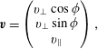 $$\begin{eqnarray}\displaystyle \boldsymbol{v}=\left(\begin{array}{@{}c@{}}v_{\bot }\cos \unicode[STIX]{x1D719}\\ v_{\bot }\sin \unicode[STIX]{x1D719}\\ v_{\Vert }\end{array}\right), & & \displaystyle\end{eqnarray}$$
and the gyrating (azimuthal) angle
 $\unicode[STIX]{x1D719}=\arctan (v_{y}/v_{x})$
. The reason is that it very nicely clarifies the meaning of gyrotropy, where the distribution function and the expressions that follow are independent of the angle
$\unicode[STIX]{x1D719}=\arctan (v_{y}/v_{x})$
. The reason is that it very nicely clarifies the meaning of gyrotropy, where the distribution function and the expressions that follow are independent of the angle
 $\unicode[STIX]{x1D719}$
. The velocity gradient in the cylindrical coordinate system reads
$\unicode[STIX]{x1D719}$
. The velocity gradient in the cylindrical coordinate system reads
 $$\begin{eqnarray}\unicode[STIX]{x1D735}_{v}=\hat{\boldsymbol{v}}_{\bot }\frac{\unicode[STIX]{x2202}}{\unicode[STIX]{x2202}v_{\bot }}+\hat{\unicode[STIX]{x1D753}}\frac{1}{v_{\bot }}\frac{\unicode[STIX]{x2202}}{\unicode[STIX]{x2202}\unicode[STIX]{x1D719}}+\hat{\boldsymbol{v}}_{\Vert }\frac{\unicode[STIX]{x2202}}{\unicode[STIX]{x2202}v_{\Vert }},\end{eqnarray}$$
where the unit vectors
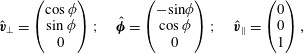 $$\begin{eqnarray}\displaystyle \hat{\boldsymbol{v}}_{\bot }=\left(\begin{array}{@{}c@{}}\cos \unicode[STIX]{x1D719}\\ \sin \unicode[STIX]{x1D719}\\ 0\end{array}\right);\quad \hat{\unicode[STIX]{x1D753}}=\left(\begin{array}{@{}c@{}}-\text{sin}\unicode[STIX]{x1D719}\\ \cos \unicode[STIX]{x1D719}\\ 0\end{array}\right);\quad \hat{\boldsymbol{v}}_{\Vert }=\left(\begin{array}{@{}c@{}}0\\ 0\\ 1\end{array}\right), & & \displaystyle\end{eqnarray}$$
so the velocity gradient is
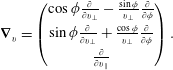 $$\begin{eqnarray}\displaystyle \unicode[STIX]{x1D735}_{v}=\left(\begin{array}{@{}c@{}}\cos \unicode[STIX]{x1D719}{\textstyle \frac{\unicode[STIX]{x2202}}{\unicode[STIX]{x2202}v_{\bot }}}-{\textstyle \frac{\sin \unicode[STIX]{x1D719}}{v_{\bot }}}{\textstyle \frac{\unicode[STIX]{x2202}}{\unicode[STIX]{x2202}\unicode[STIX]{x1D719}}}\\ \sin \unicode[STIX]{x1D719}{\textstyle \frac{\unicode[STIX]{x2202}}{\unicode[STIX]{x2202}v_{\bot }}}+{\textstyle \frac{\cos \unicode[STIX]{x1D719}}{v_{\bot }}}{\textstyle \frac{\unicode[STIX]{x2202}}{\unicode[STIX]{x2202}\unicode[STIX]{x1D719}}}\\ {\textstyle \frac{\unicode[STIX]{x2202}}{\unicode[STIX]{x2202}v_{\Vert }}}\end{array}\right). & & \displaystyle\end{eqnarray}$$
A straightforward calculation with
 $\boldsymbol{B}_{0}=(0,0,B_{0})$
yields
$\boldsymbol{B}_{0}=(0,0,B_{0})$
yields
 $$\begin{eqnarray}\displaystyle \boldsymbol{v}\times \boldsymbol{B}_{0}=B_{0}\left(\begin{array}{@{}c@{}}v_{\bot }\sin \unicode[STIX]{x1D719}\\ -v_{\bot }\cos \unicode[STIX]{x1D719}\\ 0\end{array}\right), & & \displaystyle\end{eqnarray}$$
which further implies
 $$\begin{eqnarray}\displaystyle (\boldsymbol{v}\times \boldsymbol{B}_{0})\boldsymbol{\cdot }\unicode[STIX]{x1D735}_{v} & = & \displaystyle v_{\bot }\sin \unicode[STIX]{x1D719}B_{0}\left(\cos \unicode[STIX]{x1D719}\frac{\unicode[STIX]{x2202}}{\unicode[STIX]{x2202}v_{\bot }}-\frac{\sin \unicode[STIX]{x1D719}}{v_{\bot }}\frac{\unicode[STIX]{x2202}}{\unicode[STIX]{x2202}\unicode[STIX]{x1D719}}\right)\nonumber\\ \displaystyle & & \displaystyle -\,v_{\bot }\cos \unicode[STIX]{x1D719}B_{0}\left(\sin \unicode[STIX]{x1D719}\frac{\unicode[STIX]{x2202}}{\unicode[STIX]{x2202}v_{\bot }}+\frac{\cos \unicode[STIX]{x1D719}}{v_{\bot }}\frac{\unicode[STIX]{x2202}}{\unicode[STIX]{x2202}\unicode[STIX]{x1D719}}\right)\nonumber\\ \displaystyle & = & \displaystyle -B_{0}\sin ^{2}\unicode[STIX]{x1D719}\frac{\unicode[STIX]{x2202}}{\unicode[STIX]{x2202}\unicode[STIX]{x1D719}}-B_{0}\cos ^{2}\unicode[STIX]{x1D719}\frac{\unicode[STIX]{x2202}}{\unicode[STIX]{x2202}\unicode[STIX]{x1D719}}=-B_{0}\frac{\unicode[STIX]{x2202}}{\unicode[STIX]{x2202}\unicode[STIX]{x1D719}}.\end{eqnarray}$$
Now we need to expand the Vlasov equation (2.1) around some equilibrium distribution function
 $f_{0}$
, i.e. the entire distribution function is separated to two parts as
$f_{0}$
, i.e. the entire distribution function is separated to two parts as
 $f=f_{0}+f^{(1)}$
. For the distribution function, we drop the species index
$f=f_{0}+f^{(1)}$
. For the distribution function, we drop the species index
 $r$
. The magnetic field is separated as
$r$
. The magnetic field is separated as
 $\boldsymbol{B}=\boldsymbol{B}_{0}+\boldsymbol{B}^{(1)}$
, where
$\boldsymbol{B}=\boldsymbol{B}_{0}+\boldsymbol{B}^{(1)}$
, where
 $\boldsymbol{B}_{0}=B_{0}\hat{\boldsymbol{z}}$
, and the electric field as
$\boldsymbol{B}_{0}=B_{0}\hat{\boldsymbol{z}}$
, and the electric field as
 $\boldsymbol{E}=\boldsymbol{E}_{0}+\boldsymbol{E}^{(1)}$
, but since there is no large-scale electric field in the system,
$\boldsymbol{E}=\boldsymbol{E}_{0}+\boldsymbol{E}^{(1)}$
, but since there is no large-scale electric field in the system,
 $\boldsymbol{E}_{0}=0$
.
$\boldsymbol{E}_{0}=0$
.
The most important principle that is usually not emphasized enough, is that the kinetic velocity
 $v$
is an independent quantity, and is not linearized. The entire Vlasov equation reads
$v$
is an independent quantity, and is not linearized. The entire Vlasov equation reads
 $$\begin{eqnarray}\frac{\unicode[STIX]{x2202}(f_{0}+f^{(1)})}{\unicode[STIX]{x2202}t}+\boldsymbol{v}\boldsymbol{\cdot }\unicode[STIX]{x1D735}(f_{0}+f^{(1)})+\frac{q_{r}}{m_{r}}\left[\boldsymbol{E}^{(1)}+\frac{1}{c}\boldsymbol{v}\times (\boldsymbol{B}_{0}+\boldsymbol{B}^{(1)})\right]\boldsymbol{\cdot }\unicode[STIX]{x1D735}_{v}(f_{0}+f^{(1)})=0,\end{eqnarray}$$
or equivalently by using the
 $r$
-species cyclotron frequency
$r$
-species cyclotron frequency
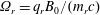 $\unicode[STIX]{x1D6FA}_{r}=q_{r}B_{0}/(m_{r}c)$
 $$\begin{eqnarray}\displaystyle & & \displaystyle \frac{\unicode[STIX]{x2202}(f_{0}+f^{(1)})}{\unicode[STIX]{x2202}t}+\boldsymbol{v}\boldsymbol{\cdot }\unicode[STIX]{x1D735}(f_{0}+f^{(1)})+\frac{q_{r}}{m_{r}}\boldsymbol{E}^{(1)}\boldsymbol{\cdot }\unicode[STIX]{x1D735}_{v}(f_{0}+f^{(1)})\nonumber\\ \displaystyle & & \displaystyle \qquad +\,\unicode[STIX]{x1D6FA}_{r}\left[\boldsymbol{v}\times \left(\hat{\boldsymbol{z}}+\frac{\boldsymbol{B}^{(1)}}{B_{0}}\right)\right]\boldsymbol{\cdot }\unicode[STIX]{x1D735}_{v}(f_{0}+f^{(1)})=0.\end{eqnarray}$$
The Vlasov equation is now expanded (i.e. linearized) by assuming that the ‘(1)’ components are small, and that terms containing 2 small ‘(1)’ quantities can be neglected. At the leading order, the situation is similar as many times before, i.e. at very low frequencies
 $(\unicode[STIX]{x1D714}\ll \unicode[STIX]{x1D6FA}_{r})$
and very long spatial scales, the term proportional to
$(\unicode[STIX]{x1D714}\ll \unicode[STIX]{x1D6FA}_{r})$
and very long spatial scales, the term proportional to
 $\unicode[STIX]{x1D6FA}_{r}$
dominates and must be by itself equal to zero
$\unicode[STIX]{x1D6FA}_{r}$
dominates and must be by itself equal to zero
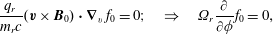 $$\begin{eqnarray}\frac{q_{r}}{m_{r}c}(\boldsymbol{v}\times \boldsymbol{B}_{0})\boldsymbol{\cdot }\unicode[STIX]{x1D735}_{v}\,f_{0}=0;\quad \Rightarrow \quad \unicode[STIX]{x1D6FA}_{r}\frac{\unicode[STIX]{x2202}}{\unicode[STIX]{x2202}\unicode[STIX]{x1D719}}f_{0}=0,\end{eqnarray}$$
where in the last step we used already calculated identity (2.7). The obtained result implies that at the longest spatial scales, the distribution function cannot depend on the azimuthal angle
 $\unicode[STIX]{x1D719}$
, or in another words, the distribution function must be isotropic in the perpendicular velocity components and can depend only on
$\unicode[STIX]{x1D719}$
, or in another words, the distribution function must be isotropic in the perpendicular velocity components and can depend only on
 $v_{x}^{2}+v_{y}^{2}=v_{\bot }^{2}$
, i.e. the distribution function must be gyrotropic. The second most important principle for doing the linear kinetic hierarchy is to realize that the hierarchy is linear, and all the quantities will have to be linearized. Additionally, we are interested only in a simplified case where the plasma is perturbed around a homogeneous equilibrium state, and we can assume that the equilibrium
$v_{x}^{2}+v_{y}^{2}=v_{\bot }^{2}$
, i.e. the distribution function must be gyrotropic. The second most important principle for doing the linear kinetic hierarchy is to realize that the hierarchy is linear, and all the quantities will have to be linearized. Additionally, we are interested only in a simplified case where the plasma is perturbed around a homogeneous equilibrium state, and we can assume that the equilibrium
 $f_{0}$
does not depend on time and position, so that
$f_{0}$
does not depend on time and position, so that
 $\unicode[STIX]{x2202}f_{0}/\unicode[STIX]{x2202}t=0$
and
$\unicode[STIX]{x2202}f_{0}/\unicode[STIX]{x2202}t=0$
and
 $\unicode[STIX]{x1D735}f_{0}=0$
. Therefore, the distribution
$\unicode[STIX]{x1D735}f_{0}=0$
. Therefore, the distribution
 $f_{0}$
contains only density
$f_{0}$
contains only density
 $n_{0}$
that is not
$n_{0}$
that is not
 $(t,\boldsymbol{x})$
dependent, or in another words
$(t,\boldsymbol{x})$
dependent, or in another words
 $f(\boldsymbol{x},\boldsymbol{v},t)=f_{0}(\boldsymbol{v})+f^{(1)}(\boldsymbol{x},\boldsymbol{v},t)$
. Perhaps a different way of looking at it is that the
$f(\boldsymbol{x},\boldsymbol{v},t)=f_{0}(\boldsymbol{v})+f^{(1)}(\boldsymbol{x},\boldsymbol{v},t)$
. Perhaps a different way of looking at it is that the
 $f_{0}$
must satisfy the leading-order Vlasov equation
$f_{0}$
must satisfy the leading-order Vlasov equation
 $$\begin{eqnarray}\frac{\unicode[STIX]{x2202}f_{0}}{\unicode[STIX]{x2202}t}+\boldsymbol{v}\boldsymbol{\cdot }\unicode[STIX]{x1D735}f_{0}+\frac{q_{r}}{m_{r}}\left[\boldsymbol{E}_{0}+\frac{1}{c}\boldsymbol{v}\times \boldsymbol{B}_{0}\right]\boldsymbol{\cdot }\unicode[STIX]{x1D735}_{v}\,f_{0}=0,\end{eqnarray}$$
which at long spatial scales and low frequencies further implies gyrotropy (2.10) and
 $\boldsymbol{E}_{0}=0$
, together with
$\boldsymbol{E}_{0}=0$
, together with
 $\unicode[STIX]{x2202}f_{0}/\unicode[STIX]{x2202}t+\boldsymbol{v}\boldsymbol{\cdot }\unicode[STIX]{x1D735}f_{0}=0$
.
$\unicode[STIX]{x2202}f_{0}/\unicode[STIX]{x2202}t+\boldsymbol{v}\boldsymbol{\cdot }\unicode[STIX]{x1D735}f_{0}=0$
.
Terms that contain 2 small
 $(1)$
quantities in (2.8) can be neglected, and putting the
$(1)$
quantities in (2.8) can be neglected, and putting the
 $f^{(1)}$
contributions to the left-hand side and the
$f^{(1)}$
contributions to the left-hand side and the
 $f_{0}$
contributions to the right-hand side yields
$f_{0}$
contributions to the right-hand side yields
 $$\begin{eqnarray}\frac{\unicode[STIX]{x2202}f^{(1)}}{\unicode[STIX]{x2202}t}+\boldsymbol{v}\boldsymbol{\cdot }\unicode[STIX]{x1D735}f^{(1)}+\frac{q_{r}}{m_{r}c}(\boldsymbol{v}\times \boldsymbol{B}_{0})\boldsymbol{\cdot }\unicode[STIX]{x1D735}_{v}\,f^{(1)}=-\frac{q_{r}}{m_{r}}\left[\boldsymbol{E}^{(1)}+\frac{1}{c}\boldsymbol{v}\times \boldsymbol{B}^{(1)}\right]\boldsymbol{\cdot }\unicode[STIX]{x1D735}_{v}\,f_{0}.\end{eqnarray}$$
This is the starting equation that expresses
 $f^{(1)}$
with respect to
$f^{(1)}$
with respect to
 $f_{0}$
and that is used in plasma physics books to derive the kinetic dispersion relation for waves in hot magnetized plasmas. The second term on the left-hand side
$f_{0}$
and that is used in plasma physics books to derive the kinetic dispersion relation for waves in hot magnetized plasmas. The second term on the left-hand side
 $\boldsymbol{v}\boldsymbol{\cdot }\unicode[STIX]{x1D735}f^{(1)}$
, introduces the simplest forms of Landau damping. The most complicated term, by far, is the third term
$\boldsymbol{v}\boldsymbol{\cdot }\unicode[STIX]{x1D735}f^{(1)}$
, introduces the simplest forms of Landau damping. The most complicated term, by far, is the third term
 $\unicode[STIX]{x1D6FA}_{r}(\boldsymbol{v}\times \boldsymbol{B}_{0}/B_{0})\boldsymbol{\cdot }\unicode[STIX]{x1D735}_{v}\,f^{(1)}$
, since it introduces non-gyrotropic
$\unicode[STIX]{x1D6FA}_{r}(\boldsymbol{v}\times \boldsymbol{B}_{0}/B_{0})\boldsymbol{\cdot }\unicode[STIX]{x1D735}_{v}\,f^{(1)}$
, since it introduces non-gyrotropic
 $f^{(1)}$
effects. This term introduces the complicated integration around the unperturbed orbit with associated sums over expressions containing Bessel functions, that are found in the full kinetic dispersion relations. It is this third term that makes the collisionless damping (and the kinetic theory) a very complicated process, even at the linear level. Without this third term, life would much easier, and Landau fluid models would be an excellent match for a full kinetic description, at least at the linear level.
$f^{(1)}$
effects. This term introduces the complicated integration around the unperturbed orbit with associated sums over expressions containing Bessel functions, that are found in the full kinetic dispersion relations. It is this third term that makes the collisionless damping (and the kinetic theory) a very complicated process, even at the linear level. Without this third term, life would much easier, and Landau fluid models would be an excellent match for a full kinetic description, at least at the linear level.
The third term is obviously equal to zero if the
 $f^{(1)}$
distribution function is assumed to be strictly gyrotropic (see (2.7)). Or, we can just neglect the term by hand, assuming that we are at low frequencies and that
$f^{(1)}$
distribution function is assumed to be strictly gyrotropic (see (2.7)). Or, we can just neglect the term by hand, assuming that we are at low frequencies and that
 $\unicode[STIX]{x1D714}\ll \unicode[STIX]{x1D6FA}$
, meaning, if we apply an ‘overly strict’ and slightly ad hoc performed low-frequency limit. However, as we will see later in the 3-D geometry section, it turns out that even if a strictly gyrotropic
$\unicode[STIX]{x1D714}\ll \unicode[STIX]{x1D6FA}$
, meaning, if we apply an ‘overly strict’ and slightly ad hoc performed low-frequency limit. However, as we will see later in the 3-D geometry section, it turns out that even if a strictly gyrotropic
 $f^{(1)}$
is assumed, the third term cannot be just eliminated from the onset. To obtain the correct
$f^{(1)}$
is assumed, the third term cannot be just eliminated from the onset. To obtain the correct
 $f^{(1)}$
in the gyrotropic limit the third term has to be retained and the integration around the unperturbed orbit performed. Only then can the term be eliminated in a limit. It is emphasized that the sophisticated Landau fluid models of Passot & Sulem (Reference Passot and Sulem2007), that we do not address here, do not neglect this third term and these models do not assume the
$f^{(1)}$
in the gyrotropic limit the third term has to be retained and the integration around the unperturbed orbit performed. Only then can the term be eliminated in a limit. It is emphasized that the sophisticated Landau fluid models of Passot & Sulem (Reference Passot and Sulem2007), that we do not address here, do not neglect this third term and these models do not assume the
 $f^{(1)}$
to be gyrotropic. It is exactly the deviations from gyrotropy that introduce the Bessel functions found in kinetic theory and sophisticated Landau fluid models.
$f^{(1)}$
to be gyrotropic. It is exactly the deviations from gyrotropy that introduce the Bessel functions found in kinetic theory and sophisticated Landau fluid models.
Now, for a moment we do not perform any calculations, and just reformulate the important equation (2.12). The first-order fields are typically transformed to Fourier space
 $({\sim}e^{i\boldsymbol{k}\boldsymbol{\cdot }\boldsymbol{x}-i\unicode[STIX]{x1D714}t})$
, but we will postpone that for now. By defining the operator
$({\sim}e^{i\boldsymbol{k}\boldsymbol{\cdot }\boldsymbol{x}-i\unicode[STIX]{x1D714}t})$
, but we will postpone that for now. By defining the operator
 $$\begin{eqnarray}\frac{\text{D}}{\text{D}t}\equiv \frac{\unicode[STIX]{x2202}}{\unicode[STIX]{x2202}t}+\boldsymbol{v}\boldsymbol{\cdot }\unicode[STIX]{x1D735}+\frac{q_{r}}{m_{r}c}(\boldsymbol{v}\times \boldsymbol{B}_{0})\boldsymbol{\cdot }\unicode[STIX]{x1D735}_{v},\end{eqnarray}$$
that represents a rate of change along an unperturbed orbit (zero-order trajectory), the equation is rewritten as
 $$\begin{eqnarray}\frac{\text{D}f^{(1)}}{\text{D}t}=-\frac{q_{r}}{m_{r}}\left[\boldsymbol{E}^{(1)}+\frac{1}{c}\boldsymbol{v}\times \boldsymbol{B}^{(1)}\right]\boldsymbol{\cdot }\unicode[STIX]{x1D735}_{v}\,f_{0}.\end{eqnarray}$$
To obtain the
 $f^{(1)}$
, one therefore has to calculate the integral of the above equation, where also the integration of the right-hand side must be naturally done along the zero-order trajectory (along the unperturbed orbit) in order to cancel the
$f^{(1)}$
, one therefore has to calculate the integral of the above equation, where also the integration of the right-hand side must be naturally done along the zero-order trajectory (along the unperturbed orbit) in order to cancel the
 $\text{d}/\text{d}t$
on the left-hand side. The integration is denoted with prime quantities, and the integral is performed along
$\text{d}/\text{d}t$
on the left-hand side. The integration is denoted with prime quantities, and the integral is performed along
 $\text{d}t^{\prime }$
. If the integral is performed from time
$\text{d}t^{\prime }$
. If the integral is performed from time
 $t^{\prime }=t_{0}$
to
$t^{\prime }=t_{0}$
to
 $t^{\prime }=t$
, the integration of the left-hand side yields
$t^{\prime }=t$
, the integration of the left-hand side yields
 $f^{(1)}(\boldsymbol{x},\boldsymbol{v},t)-f^{(1)}(\boldsymbol{x},\boldsymbol{v},t_{0})$
, i.e. the result depends on the initial condition at time
$f^{(1)}(\boldsymbol{x},\boldsymbol{v},t)-f^{(1)}(\boldsymbol{x},\boldsymbol{v},t_{0})$
, i.e. the result depends on the initial condition at time
 $t_{0}$
. To remove this dependence, the integral is performed from
$t_{0}$
. To remove this dependence, the integral is performed from
 $t_{0}=-\infty$
and it is typically stated that, in this case, the initial condition
$t_{0}=-\infty$
and it is typically stated that, in this case, the initial condition
 $f^{(1)}(\boldsymbol{x},\boldsymbol{v},-\infty )$
can be neglected. (This is however not that obvious and, for example, Stix have a rather long discussion in this regard on page 249). The distribution function
$f^{(1)}(\boldsymbol{x},\boldsymbol{v},-\infty )$
can be neglected. (This is however not that obvious and, for example, Stix have a rather long discussion in this regard on page 249). The distribution function
 $f^{(1)}(\boldsymbol{x},\boldsymbol{v},t)$
is therefore obtained by performing the integral
$f^{(1)}(\boldsymbol{x},\boldsymbol{v},t)$
is therefore obtained by performing the integral
 $$\begin{eqnarray}f^{(1)}(\boldsymbol{x},\boldsymbol{v},t)=-\frac{q_{r}}{m_{r}}\int _{-\infty }^{t}\left[\boldsymbol{E}^{(1)}(\boldsymbol{x}^{\prime },t^{\prime })+\frac{1}{c}\boldsymbol{v}^{\prime }\times \boldsymbol{B}^{(1)}(\boldsymbol{x}^{\prime },t^{\prime })\right]\boldsymbol{\cdot }\unicode[STIX]{x1D735}_{v^{\prime }}f_{0}(\boldsymbol{v}^{\prime })\,\text{d}t^{\prime }.\end{eqnarray}$$
The calculation of this integral is cumbersome because of the required change of coordinates. We want to get the final
 $f^{(1)}$
expression and we will repeat the algebra concerning how to obtain it, but before doing that, let us consider the simplest possible case.
$f^{(1)}$
expression and we will repeat the algebra concerning how to obtain it, but before doing that, let us consider the simplest possible case.
2.1 The simplest case: 1-D geometry, Maxwellian
 $f_{0}$

Let us consider a particular situation, when (for whatever reason) the third term on the left-hand side of equation (2.12) disappears, i.e. let us briefly consider
 $$\begin{eqnarray}(\boldsymbol{v}\times \boldsymbol{B}_{0})\boldsymbol{\cdot }\unicode[STIX]{x1D735}_{v}\,f^{(1)}=0,\end{eqnarray}$$
which according to (2.10) implies that
 $f^{(1)}$
is gyrotropic (it does not depend on the angle
$f^{(1)}$
is gyrotropic (it does not depend on the angle
 $\unicode[STIX]{x1D719}$
). Let us also consider the even more special case in which
$\unicode[STIX]{x1D719}$
). Let us also consider the even more special case in which
 $f_{0}$
is isotropic. In such a case, that is a specific case of (2.16), the direction of
$f_{0}$
is isotropic. In such a case, that is a specific case of (2.16), the direction of
 $\boldsymbol{B}^{(1)}$
does not matter at all for
$\boldsymbol{B}^{(1)}$
does not matter at all for
 $f_{0}$
and naturally
$f_{0}$
and naturally
 $$\begin{eqnarray}(\boldsymbol{v}\times \boldsymbol{B}^{(1)})\boldsymbol{\cdot }\unicode[STIX]{x1D735}_{v}\,f_{0}=0.\end{eqnarray}$$
To quickly double check the correctness of the above expression, for isotropic
 $f_{0}(v)$
the velocity gradient is given by
$f_{0}(v)$
the velocity gradient is given by
 $\unicode[STIX]{x2202}f_{0}/\unicode[STIX]{x2202}v_{i}=(\unicode[STIX]{x2202}f_{0}/\unicode[STIX]{x2202}v)(\unicode[STIX]{x2202}v/\unicode[STIX]{x2202}v_{i})=f_{0}^{\prime }v_{i}/v$
and the velocity gradient
$\unicode[STIX]{x2202}f_{0}/\unicode[STIX]{x2202}v_{i}=(\unicode[STIX]{x2202}f_{0}/\unicode[STIX]{x2202}v)(\unicode[STIX]{x2202}v/\unicode[STIX]{x2202}v_{i})=f_{0}^{\prime }v_{i}/v$
and the velocity gradient
 $\unicode[STIX]{x1D735}_{v}\,f_{0}=f_{0}^{\prime }\hat{\boldsymbol{v}}$
is in the direction of velocity
$\unicode[STIX]{x1D735}_{v}\,f_{0}=f_{0}^{\prime }\hat{\boldsymbol{v}}$
is in the direction of velocity
 $\boldsymbol{v}$
. The result (2.17) then immediately follows since
$\boldsymbol{v}$
. The result (2.17) then immediately follows since
 $\unicode[STIX]{x1D716}_{ijk}v_{j}B_{k}^{(1)}v_{i}=0$
. The equation (2.12) therefore reduces to
$\unicode[STIX]{x1D716}_{ijk}v_{j}B_{k}^{(1)}v_{i}=0$
. The equation (2.12) therefore reduces to
 $$\begin{eqnarray}\frac{\unicode[STIX]{x2202}f^{(1)}}{\unicode[STIX]{x2202}t}+\boldsymbol{v}\boldsymbol{\cdot }\unicode[STIX]{x1D735}f^{(1)}=-\frac{q_{r}}{m_{r}}\boldsymbol{E}^{(1)}\boldsymbol{\cdot }\unicode[STIX]{x1D735}_{v}\,f_{0}.\end{eqnarray}$$
Fourier transforming the first-order quantities and
 $\unicode[STIX]{x2202}/\unicode[STIX]{x2202}t\rightarrow -i\unicode[STIX]{x1D714}$
,
$\unicode[STIX]{x2202}/\unicode[STIX]{x2202}t\rightarrow -i\unicode[STIX]{x1D714}$
,
 $\unicode[STIX]{x1D735}\rightarrow i\boldsymbol{k}$
yields
$\unicode[STIX]{x1D735}\rightarrow i\boldsymbol{k}$
yields
 $$\begin{eqnarray}(-i\unicode[STIX]{x1D714}+i\boldsymbol{v}\boldsymbol{\cdot }\boldsymbol{k})f^{(1)}=-\frac{q_{r}}{m_{r}}\boldsymbol{E}^{(1)}\boldsymbol{\cdot }\unicode[STIX]{x1D735}_{v}\,f_{0},\end{eqnarray}$$
which allows us to obtain an expression for
 $f^{(1)}$
in the form
$f^{(1)}$
in the form
 $$\begin{eqnarray}f^{(1)}=-i\frac{q_{r}}{m_{r}}\;\frac{\boldsymbol{E}^{(1)}\boldsymbol{\cdot }\unicode[STIX]{x1D735}_{v}\,f_{0}}{\unicode[STIX]{x1D714}-\boldsymbol{v}\boldsymbol{\cdot }\boldsymbol{k}}.\end{eqnarray}$$
Even though it is not necessary, it is useful to express the (electrostatic) electric field through the scalar potential
 $\boldsymbol{E}^{(1)}=-\unicode[STIX]{x1D735}\unicode[STIX]{x1D6F7}$
, which in Fourier space reads
$\boldsymbol{E}^{(1)}=-\unicode[STIX]{x1D735}\unicode[STIX]{x1D6F7}$
, which in Fourier space reads
 $\boldsymbol{E}^{(1)}=-i\boldsymbol{k}\unicode[STIX]{x1D6F7}$
, yielding
$\boldsymbol{E}^{(1)}=-i\boldsymbol{k}\unicode[STIX]{x1D6F7}$
, yielding
 $$\begin{eqnarray}f^{(1)}=-\frac{q_{r}}{m_{r}}\unicode[STIX]{x1D6F7}\;\frac{\boldsymbol{k}\boldsymbol{\cdot }\unicode[STIX]{x1D735}_{v}\,f_{0}}{\unicode[STIX]{x1D714}-\boldsymbol{v}\boldsymbol{\cdot }\boldsymbol{k}}.\end{eqnarray}$$
Now, we want to integrate
 $f^{(1)}$
, and obtain the linear ‘kinetic’ moments for density, velocity (current), pressure (temperature), heat flux and the fourth-order moment
$f^{(1)}$
, and obtain the linear ‘kinetic’ moments for density, velocity (current), pressure (temperature), heat flux and the fourth-order moment
 $r$
(or the correction
$r$
(or the correction
 $\tilde{r}$
). To continue, we have to prescribe some distribution function
$\tilde{r}$
). To continue, we have to prescribe some distribution function
 $f_{0}$
.
$f_{0}$
.
The 3-D (isotropic) Maxwellian distribution is
 $$\begin{eqnarray}f_{0r}=n_{0r}\left(\frac{\unicode[STIX]{x1D6FC}_{r}}{\unicode[STIX]{x03C0}}\right)^{3/2}e^{-\unicode[STIX]{x1D6FC}_{r}v^{2}},\end{eqnarray}$$
where the isotropic
 $v^{2}=v_{x}^{2}+v_{y}^{2}+v_{z}^{2}$
and
$v^{2}=v_{x}^{2}+v_{y}^{2}+v_{z}^{2}$
and
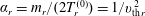 $\unicode[STIX]{x1D6FC}_{r}=m_{r}/(2T_{r}^{(0)})=1/v_{\text{th}r}^{2}$
. For simplicity, let us drop the species index
$\unicode[STIX]{x1D6FC}_{r}=m_{r}/(2T_{r}^{(0)})=1/v_{\text{th}r}^{2}$
. For simplicity, let us drop the species index
 $r$
, except for the charge
$r$
, except for the charge
 $q_{r}$
. The velocity gradient
$q_{r}$
. The velocity gradient
 $$\begin{eqnarray}\displaystyle {\displaystyle \frac{\unicode[STIX]{x2202}f_{0}}{\unicode[STIX]{x2202}v_{i}}} & = & \displaystyle n_{0}\left({\displaystyle \frac{\unicode[STIX]{x1D6FC}}{\unicode[STIX]{x03C0}}}\right)^{3/2}(-\unicode[STIX]{x1D6FC})2v_{i}e^{-\unicode[STIX]{x1D6FC}v^{2}}=-2\unicode[STIX]{x1D6FC}v_{i}f_{0}=-{\displaystyle \frac{m}{T^{(0)}}}v_{i}f_{0},\nonumber\\ \displaystyle \unicode[STIX]{x1D735}_{v}\,f_{0} & = & \displaystyle -{\displaystyle \frac{m}{T^{(0)}}}\boldsymbol{v}f_{0}.\end{eqnarray}$$
Therefore, for a Maxwellian
 $$\begin{eqnarray}f^{(1)}=+\frac{q_{r}}{T^{(0)}}\unicode[STIX]{x1D6F7}\;\frac{\boldsymbol{k}\boldsymbol{\cdot }\boldsymbol{v}}{\unicode[STIX]{x1D714}-\boldsymbol{v}\boldsymbol{\cdot }\boldsymbol{k}}f_{0}.\end{eqnarray}$$
Before continuing, let us slightly rearrange the above expression for
 $f^{(1)}$
and add
$f^{(1)}$
and add
 $0=\unicode[STIX]{x1D714}-\unicode[STIX]{x1D714}$
to the numerator, otherwise we will have to do this each time, when calculating the higher-order moments. The rearrangement yields
$0=\unicode[STIX]{x1D714}-\unicode[STIX]{x1D714}$
to the numerator, otherwise we will have to do this each time, when calculating the higher-order moments. The rearrangement yields
 $$\begin{eqnarray}\displaystyle f^{(1)}=+\frac{q_{r}}{T^{(0)}}\unicode[STIX]{x1D6F7}\;\frac{\boldsymbol{k}\boldsymbol{\cdot }\boldsymbol{v}-\unicode[STIX]{x1D714}+\unicode[STIX]{x1D714}}{\unicode[STIX]{x1D714}-\boldsymbol{v}\boldsymbol{\cdot }\boldsymbol{k}}f_{0}=-\frac{q_{r}}{T^{(0)}}\unicode[STIX]{x1D6F7}\;\left(1+\frac{\unicode[STIX]{x1D714}}{\boldsymbol{v}\boldsymbol{\cdot }\boldsymbol{ k}-\unicode[STIX]{x1D714}}\right)f_{0}. & & \displaystyle\end{eqnarray}$$
For clarity, let us simplify even further and discuss the simplest possible 1-D case, for a 1-D Maxwellian distribution
 $$\begin{eqnarray}f_{0}=n_{0}\sqrt{\frac{\unicode[STIX]{x1D6FC}}{\unicode[STIX]{x03C0}}}e^{-\unicode[STIX]{x1D6FC}v^{2}};\quad \text{where }\unicode[STIX]{x1D6FC}\equiv \frac{m}{2T^{(0)}}=\frac{1}{v_{\text{th}}^{2}}.\end{eqnarray}$$
Here we consider fluctuations along the magnetic field
 $B_{0}$
and the wavenumber is therefore denoted as
$B_{0}$
and the wavenumber is therefore denoted as
 $k_{\Vert }$
. Note that the case is strictly one-dimensional, and the velocity fluctuations are along the
$k_{\Vert }$
. Note that the case is strictly one-dimensional, and the velocity fluctuations are along the
 $B_{0}$
as well. For example from the MHD perspective, we are therefore considering the parallel propagating ion-acoustic mode. The
$B_{0}$
as well. For example from the MHD perspective, we are therefore considering the parallel propagating ion-acoustic mode. The
 $f^{(1)}$
for a Maxwellian
$f^{(1)}$
for a Maxwellian
 $f_{0}$
is expressed as (dropping all the species indices ‘
$f_{0}$
is expressed as (dropping all the species indices ‘
 $r$
’ except for the charge
$r$
’ except for the charge
 $q_{r}$
)
$q_{r}$
)
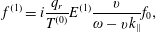 $$\begin{eqnarray}\displaystyle & \displaystyle f^{(1)}=i\frac{q_{r}}{T^{(0)}}E^{(1)}\frac{v}{\unicode[STIX]{x1D714}-vk_{\Vert }}f_{0}, & \displaystyle\end{eqnarray}$$
 $$\begin{eqnarray}\displaystyle & \displaystyle f^{(1)}=-\frac{q_{r}}{T^{(0)}}\unicode[STIX]{x1D6F7}\left(1+\frac{{\displaystyle \frac{\unicode[STIX]{x1D714}}{k_{\Vert }}}}{v-{\displaystyle \frac{\unicode[STIX]{x1D714}}{k_{\Vert }}}}\right)f_{0}. & \displaystyle\end{eqnarray}$$
Now, we are ready to calculate the velocity integrals. Let us start with the density
 $n^{(1)}$
, by integrating
$n^{(1)}$
, by integrating
 $$\begin{eqnarray}n^{(1)}=\int _{-\infty }^{\infty }f^{(1)}\,\text{d}v=-\frac{q_{r}}{T^{(0)}}\unicode[STIX]{x1D6F7}\left(\underbrace{\int _{-\infty }^{\infty }f_{0}\,\text{d}v}_{=n_{0}}+\int _{-\infty }^{\infty }\frac{{\displaystyle \frac{\unicode[STIX]{x1D714}}{k_{\Vert }}}f_{0}}{v-{\displaystyle \frac{\unicode[STIX]{x1D714}}{k_{\Vert }}}}\,\text{d}v\right).\end{eqnarray}$$
By using the prescribed Maxwellian
 $f_{0}$
, the second integral is rewritten as
$f_{0}$
, the second integral is rewritten as
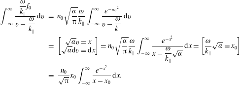 $$\begin{eqnarray}\displaystyle \int _{-\infty }^{\infty }\frac{{\displaystyle \frac{\unicode[STIX]{x1D714}}{k_{\Vert }}}f_{0}}{v-{\displaystyle \frac{\unicode[STIX]{x1D714}}{k_{\Vert }}}}\,\text{d}v & = & \displaystyle n_{0}\sqrt{\frac{\unicode[STIX]{x1D6FC}}{\unicode[STIX]{x03C0}}}\frac{\unicode[STIX]{x1D714}}{k_{\Vert }}\int _{-\infty }^{\infty }\frac{e^{-\unicode[STIX]{x1D6FC}v^{2}}}{v-{\displaystyle \frac{\unicode[STIX]{x1D714}}{k_{\Vert }}}}\,\text{d}v\nonumber\\ \displaystyle & = & \displaystyle \left[\begin{array}{@{}c@{}}\sqrt{\unicode[STIX]{x1D6FC}}v=x\\ \sqrt{\unicode[STIX]{x1D6FC}}\text{d}v=\text{d}x\end{array}\right]=n_{0}\sqrt{\frac{\unicode[STIX]{x1D6FC}}{\unicode[STIX]{x03C0}}}\frac{\unicode[STIX]{x1D714}}{k_{\Vert }}\int _{-\infty }^{\infty }\frac{e^{-x^{2}}}{x-{\displaystyle \frac{\unicode[STIX]{x1D714}}{k_{\Vert }}}\sqrt{\unicode[STIX]{x1D6FC}}}\,\text{d}x=\left[\frac{\unicode[STIX]{x1D714}}{k_{\Vert }}\sqrt{\unicode[STIX]{x1D6FC}}\equiv x_{0}\right]\nonumber\\ \displaystyle & = & \displaystyle \frac{n_{0}}{\sqrt{\unicode[STIX]{x03C0}}}x_{0}\int _{-\infty }^{\infty }\frac{e^{-x^{2}}}{x-x_{0}}\,\text{d}x.\end{eqnarray}$$
The notation
 $[\cdots \,]$
just indicates change of a variable. We purposely wrote the integral with
$[\cdots \,]$
just indicates change of a variable. We purposely wrote the integral with
 $$\begin{eqnarray}x_{0}\equiv \frac{\unicode[STIX]{x1D714}}{k_{\Vert }}\sqrt{\unicode[STIX]{x1D6FC}}=\frac{\unicode[STIX]{x1D714}}{k_{\Vert }v_{\text{th}}},\end{eqnarray}$$
instead of the usual
 $\unicode[STIX]{x1D701}$
, since we want to define
$\unicode[STIX]{x1D701}$
, since we want to define
 $\unicode[STIX]{x1D701}$
slightly differently. The integral is related to the famous plasma dispersion function
$\unicode[STIX]{x1D701}$
slightly differently. The integral is related to the famous plasma dispersion function
 $Z(\unicode[STIX]{x1D701})$
, that is responsible for the famous Landau damping. Each plasma physics book devotes many pages to the discussion of Landau damping, that was first correctly described by Landau (Reference Landau1946), by considering an initial value problem and using Laplace transforms. It was later shown by van Kampen (Reference van Kampen1955), that the Landau damping can be indeed obtained by using Fourier analysis. We refer the reader for example to books by Swanson, Stix, Akhiezer, Gary, Gurnett and Bhattacharjee, Fitzpatrick, etc. Let us call the integral (2.30) the ‘Landau integral’. Nevertheless, the very-well-known secret is that, even if one is armed with all these excellent books, the Landau damping effect can still be very confusing (even at the linear level). We did not find any secret recipe that explains the Landau damping in a simplified and different way, and the reader is referred to the thick plasma physics books. Here, we want to concentrate only how to express the integral (2.30) through the plasma dispersion function.
$Z(\unicode[STIX]{x1D701})$
, that is responsible for the famous Landau damping. Each plasma physics book devotes many pages to the discussion of Landau damping, that was first correctly described by Landau (Reference Landau1946), by considering an initial value problem and using Laplace transforms. It was later shown by van Kampen (Reference van Kampen1955), that the Landau damping can be indeed obtained by using Fourier analysis. We refer the reader for example to books by Swanson, Stix, Akhiezer, Gary, Gurnett and Bhattacharjee, Fitzpatrick, etc. Let us call the integral (2.30) the ‘Landau integral’. Nevertheless, the very-well-known secret is that, even if one is armed with all these excellent books, the Landau damping effect can still be very confusing (even at the linear level). We did not find any secret recipe that explains the Landau damping in a simplified and different way, and the reader is referred to the thick plasma physics books. Here, we want to concentrate only how to express the integral (2.30) through the plasma dispersion function.
Since the Landau integral can be very confusing and boring to explain, to increase the ‘pedagogical’ value of this text, let us talk a bit more freely on the next few pages. The plasma dispersion function can be defined with a short definition
 $$\begin{eqnarray}Z(\unicode[STIX]{x1D701})\equiv \frac{1}{\sqrt{\unicode[STIX]{x03C0}}}\int _{-\infty }^{\infty }\frac{e^{-x^{2}}}{x-\unicode[STIX]{x1D701}}\,\text{d}x,\quad \text{for }\text{Im}(\unicode[STIX]{x1D701})>0.\end{eqnarray}$$
In the definition of
 $x_{0}$
, the thermal speed
$x_{0}$
, the thermal speed
 $v_{\text{th}}$
is always a positive real number, and we do not have to worry about it. Now, considering the specific case
$v_{\text{th}}$
is always a positive real number, and we do not have to worry about it. Now, considering the specific case
 $k_{\Vert }>0$
and
$k_{\Vert }>0$
and
 $\text{Im}(\unicode[STIX]{x1D714})>0$
, where we indeed have
$\text{Im}(\unicode[STIX]{x1D714})>0$
, where we indeed have
 $\text{Im}(x_{0})>0$
, we can directly use the plasma dispersion function and the result of the Landau integral (2.30) is
$\text{Im}(x_{0})>0$
, we can directly use the plasma dispersion function and the result of the Landau integral (2.30) is
 $n_{0}x_{0}Z(x_{0})$
. For this case, we are done. Really? Yes, there is nothing else we can do for this case, we calculated the Landau integral. Reeeaallyy?? Yes, because the Landau integral cannot be analytically ‘calculated’, the integral cannot be expressed through elementary functions, unless the
$n_{0}x_{0}Z(x_{0})$
. For this case, we are done. Really? Yes, there is nothing else we can do for this case, we calculated the Landau integral. Reeeaallyy?? Yes, because the Landau integral cannot be analytically ‘calculated’, the integral cannot be expressed through elementary functions, unless the
 $Z(\unicode[STIX]{x1D701})$
function is somehow simplified, for example by expansion for cases
$Z(\unicode[STIX]{x1D701})$
function is somehow simplified, for example by expansion for cases
 $|\unicode[STIX]{x1D701}|\ll 1$
or
$|\unicode[STIX]{x1D701}|\ll 1$
or
 $|\unicode[STIX]{x1D701}|\gg 1$
, or by considering the weak damping limit when
$|\unicode[STIX]{x1D701}|\gg 1$
, or by considering the weak damping limit when
 $\text{Im}(x_{0})$
is small (see plasma physics books). We are not interested in these limits and the
$\text{Im}(x_{0})$
is small (see plasma physics books). We are not interested in these limits and the
 $Z(\unicode[STIX]{x1D701})$
function has to be calculated numerically or looked up in the table. We are really done here!Footnote
1
So why is the Landau integral so confusing for the other cases? It is exactly because of that – basically nothing gets ‘really calculated’.
$Z(\unicode[STIX]{x1D701})$
function has to be calculated numerically or looked up in the table. We are really done here!Footnote
1
So why is the Landau integral so confusing for the other cases? It is exactly because of that – basically nothing gets ‘really calculated’.
2.2 The dreadful Landau integral
$\int e^{-x^{2}}/(x-x_{0})\,\text{d}x$
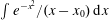
There are many reasons why the ‘Landau integral’ (2.30) can be so confusing. The first reason is, (i) that the integral (2.30) cannot be expressed by using only elementary functions. If we did not arrive at this integral in the middle of a thick plasma physics book, but instead encountered it during our undergraduate studies of complex analysis, we would perhaps not have such a respect to this integral, and immediately attempt to calculate it by using the residue theorem. The integral appears to be so simple. Instead of calculating
 $\int _{-\infty }^{\infty }$
, we would calculate a different integral over a closed contour in the complex plane
$\int _{-\infty }^{\infty }$
, we would calculate a different integral over a closed contour in the complex plane
 $\oint _{C}$
. That integral can be calculated by using the residue theorem, that states that
$\oint _{C}$
. That integral can be calculated by using the residue theorem, that states that
 $\oint _{C}=2\unicode[STIX]{x03C0}i\sum \text{Res}$
, if the big path that encircles all the poles is counter-clockwise.Footnote
2
An equivalent statement is that the integral is equal to
$\oint _{C}=2\unicode[STIX]{x03C0}i\sum \text{Res}$
, if the big path that encircles all the poles is counter-clockwise.Footnote
2
An equivalent statement is that the integral is equal to
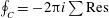 $\oint _{C}=-2\unicode[STIX]{x03C0}i\sum \text{Res}$
, if the big path that encircles all the poles is clockwise. In our case, there is always just one pole, at
$\oint _{C}=-2\unicode[STIX]{x03C0}i\sum \text{Res}$
, if the big path that encircles all the poles is clockwise. In our case, there is always just one pole, at
 $x=x_{0}$
, and the residue of
$x=x_{0}$
, and the residue of
 $e^{-x^{2}}/(x-x_{0})$
evaluated at
$e^{-x^{2}}/(x-x_{0})$
evaluated at
 $x=x_{0}$
is actually very simple, it is always
$x=x_{0}$
is actually very simple, it is always
 $$\begin{eqnarray}\underset{x=x_{0}}{\text{Res}}\;\frac{e^{-x^{2}}}{x-x_{0}}=e^{-x_{0}^{2}},\end{eqnarray}$$
regardless of the value of
 $x_{0}$
, since for a general function
$x_{0}$
, since for a general function
 $f(x)$
, the residue
$f(x)$
, the residue
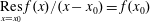 $\underset{x=x_{0}}{\text{Res}}\;f(x)/(x-x_{0})=f(x_{0})$
.
$\underset{x=x_{0}}{\text{Res}}\;f(x)/(x-x_{0})=f(x_{0})$
.
However, to make the result
 $\oint _{C}$
useful for the calculation of our integral on the real axis
$\oint _{C}$
useful for the calculation of our integral on the real axis
 $\int _{-\infty }^{\infty }$
, we need to separate the closed contour integral to
$\int _{-\infty }^{\infty }$
, we need to separate the closed contour integral to
 $\oint _{C}=\int _{-\infty }^{\infty }+\int _{\text{arc}}$
, where the
$\oint _{C}=\int _{-\infty }^{\infty }+\int _{\text{arc}}$
, where the
 $\int _{\text{arc}}$
represents the big half-circle at infinitely large radius. To preserve the direction of integration along the real axis
$\int _{\text{arc}}$
represents the big half-circle at infinitely large radius. To preserve the direction of integration along the real axis
 $\int _{-\infty }^{\infty }$
, if the pole is in the upper complex plane, i.e. if
$\int _{-\infty }^{\infty }$
, if the pole is in the upper complex plane, i.e. if
 $\text{Im}(x_{0})>0$
, we need to close the big arc contour in the upper half of the complex plane counter-clockwise. Similarly, if the pole is in the lower complex plane, i.e. if
$\text{Im}(x_{0})>0$
, we need to close the big arc contour in the upper half of the complex plane counter-clockwise. Similarly, if the pole is in the lower complex plane, i.e. if
 $\text{Im}(x_{0})<0$
, we need to close the big arc contour clockwise. Importantly, in contrast to typical examples presented in basic complex analysis classes, the arc integral
$\text{Im}(x_{0})<0$
, we need to close the big arc contour clockwise. Importantly, in contrast to typical examples presented in basic complex analysis classes, the arc integral
 $\int _{\text{arc}}$
does not disappear. The problem is, that the function
$\int _{\text{arc}}$
does not disappear. The problem is, that the function
 $f(x)=e^{-z^{2}}$
is a very strongly decaying function on the real axis (for
$f(x)=e^{-z^{2}}$
is a very strongly decaying function on the real axis (for
 $z=x\rightarrow \pm \infty$
), however, this is not true at all in the complex plane. Considering the purely Imaginary axis
$z=x\rightarrow \pm \infty$
), however, this is not true at all in the complex plane. Considering the purely Imaginary axis
 $z=\pm iy$
, the function
$z=\pm iy$
, the function
 $e^{-z^{2}}=e^{+y^{2}}$
is a very strongly diverging function as
$e^{-z^{2}}=e^{+y^{2}}$
is a very strongly diverging function as
 $y$
increases, and the arc integral
$y$
increases, and the arc integral
 $\int _{\text{arc}}$
cannot be neglected! This is a very sad news, since now we clearly see, that with
$\int _{\text{arc}}$
cannot be neglected! This is a very sad news, since now we clearly see, that with
 $\int _{\text{arc}}\neq 0$
, we will not be able to use the complex analysis to actually ‘calculate’ the Landau integral (2.30).
$\int _{\text{arc}}\neq 0$
, we will not be able to use the complex analysis to actually ‘calculate’ the Landau integral (2.30).
We note that the well-known Gaussian integral
 $I=\int _{-\infty }^{\infty }e^{-x^{2}}\,\text{d}x=\sqrt{\unicode[STIX]{x03C0}}$
, is typically calculated in the real plane by means of a trick which consists in evaluating
$I=\int _{-\infty }^{\infty }e^{-x^{2}}\,\text{d}x=\sqrt{\unicode[STIX]{x03C0}}$
, is typically calculated in the real plane by means of a trick which consists in evaluating
 $I^{2}$
in polar coordinates,
$I^{2}$
in polar coordinates,
 $I^{2}=\int _{-\infty }^{\infty }e^{-x^{2}-y^{2}}\,\text{d}x\,\text{d}y=2\unicode[STIX]{x03C0}\int _{0}^{\infty }e^{-r^{2}}r\,\text{d}r$
. The Gaussian integral can still be calculated in the complex plane by using the residue theorem, even though quite sophisticated tricks are required.Footnote
3
$I^{2}=\int _{-\infty }^{\infty }e^{-x^{2}-y^{2}}\,\text{d}x\,\text{d}y=2\unicode[STIX]{x03C0}\int _{0}^{\infty }e^{-r^{2}}r\,\text{d}r$
. The Gaussian integral can still be calculated in the complex plane by using the residue theorem, even though quite sophisticated tricks are required.Footnote
3
The second reason why Landau damping is confusing is, (ii) the necessity of analytic continuation. The third reason is very closely related to the second and it is (iii) The analytic continuation has to be done differently for
 $k_{\Vert }>0$
and for
$k_{\Vert }>0$
and for
 $k_{\Vert }<0$
. The big result of Landau (Reference Landau1946) can be summarized as follows: if
$k_{\Vert }<0$
. The big result of Landau (Reference Landau1946) can be summarized as follows: if
 $k_{\Vert }>0$
, the path of integration always has to pass below the pole
$k_{\Vert }>0$
, the path of integration always has to pass below the pole
 $x=x_{0}$
. Therefore, starting with the basic case in the upper complex plane
$x=x_{0}$
. Therefore, starting with the basic case in the upper complex plane
 $\text{Im}(x_{0})>0$
, nothing has to be done and the integration is just along the real axis. Now, if the pole is moved to the real axis, so
$\text{Im}(x_{0})>0$
, nothing has to be done and the integration is just along the real axis. Now, if the pole is moved to the real axis, so
 $\text{Im}(x_{0})=0$
, one needs to go around that pole with a tiny half-circle from below. This creates a contribution of
$\text{Im}(x_{0})=0$
, one needs to go around that pole with a tiny half-circle from below. This creates a contribution of
 $1/2$
times
$1/2$
times
 $2\unicode[STIX]{x03C0}i$
times the residue at that pole, so the contribution is
$2\unicode[STIX]{x03C0}i$
times the residue at that pole, so the contribution is
 $\unicode[STIX]{x03C0}ie^{-x_{0}^{2}}$
. If the pole
$\unicode[STIX]{x03C0}ie^{-x_{0}^{2}}$
. If the pole
 $x_{0}$
is moved further down to the lower complex plane, a full circle around the pole is required to enclose it from below, which yields a contribution of
$x_{0}$
is moved further down to the lower complex plane, a full circle around the pole is required to enclose it from below, which yields a contribution of
 $2\unicode[STIX]{x03C0}ie^{-x_{0}^{2}}$
. The situation is demonstrated in figure 1(a). The integral (2.30) for
$2\unicode[STIX]{x03C0}ie^{-x_{0}^{2}}$
. The situation is demonstrated in figure 1(a). The integral (2.30) for
 $k_{\Vert }>0$
is therefore ‘calculated’ as
$k_{\Vert }>0$
is therefore ‘calculated’ as
 $$\begin{eqnarray}\int _{C}\frac{e^{-x^{2}}}{x-x_{0}}\,\text{d}x\overset{k_{\Vert }>0}{=}\left\{\begin{array}{@{}ll@{}}\displaystyle \int _{-\infty }^{\infty }\frac{e^{-x^{2}}}{x-x_{0}}\,\text{d}x,\quad & \text{Im}(\unicode[STIX]{x1D714})>0;\text{Im}(x_{0})>0;\\ \displaystyle V.P.\int _{-\infty }^{\infty }\frac{e^{-x^{2}}}{x-x_{0}}\,\text{d}x+\unicode[STIX]{x03C0}ie^{-x_{0}^{2}},\quad & \text{Im}(\unicode[STIX]{x1D714})=0;\text{Im}(x_{0})=0;\\ \displaystyle \int _{-\infty }^{\infty }\frac{e^{-x^{2}}}{x-x_{0}}\,\text{d}x+2\unicode[STIX]{x03C0}ie^{-x_{0}^{2}},\quad & \text{Im}(\unicode[STIX]{x1D714})<0;\text{Im}(x_{0})<0.\end{array}\right.\end{eqnarray}$$
For the Cauchy principal value, we prefer the original French pronunciation ‘Valeur Principale’, abbreviated as
 $V.P$
.
$V.P$
.
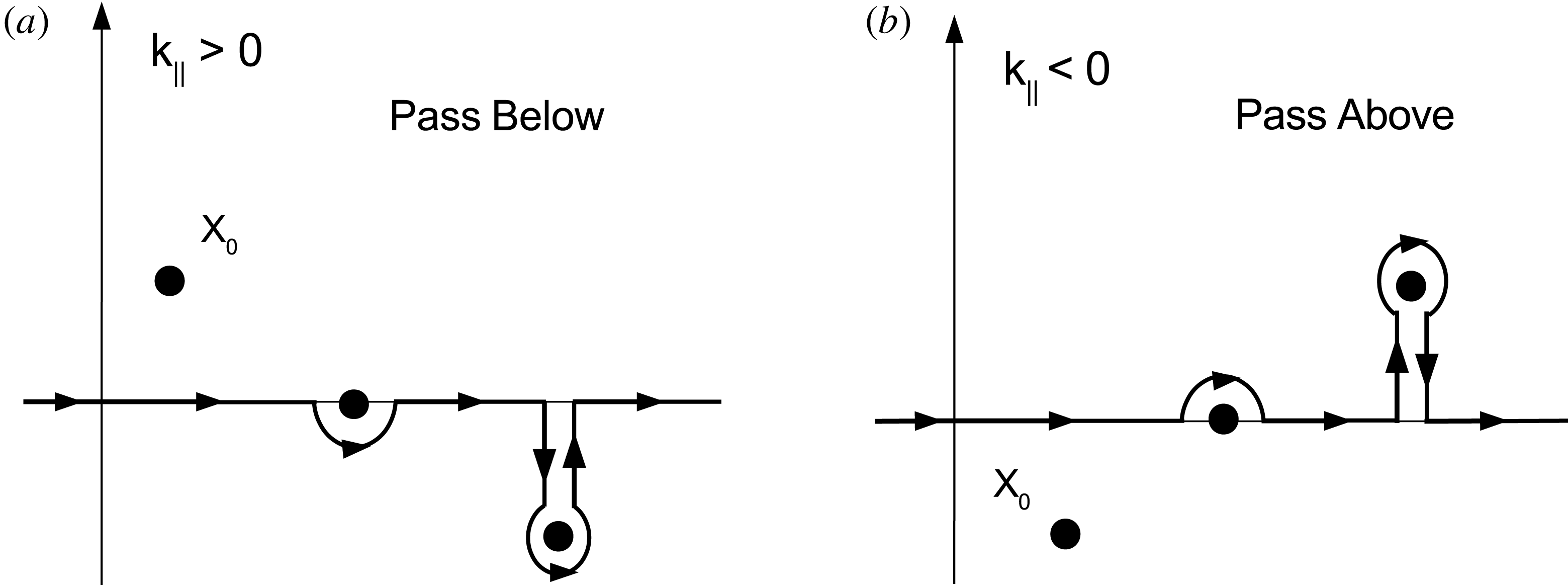
Figure 1. (a) Landau contours for
 $k_{\Vert }>0$
. (b) Landau contours for
$k_{\Vert }>0$
. (b) Landau contours for
 $k_{\Vert }<0$
.
$k_{\Vert }<0$
.
The above result is completely consistent with the definition of the plasma dispersion function, since the plasma dispersion function was developed exactly to describe this integral. One starts with the definition in the upper complex plane (2.32), and analytically continues this function to a lower complex plane, according to
 $$\begin{eqnarray}Z(\unicode[STIX]{x1D701})\equiv \frac{1}{\sqrt{\unicode[STIX]{x03C0}}}\int _{C}\frac{e^{-x^{2}}}{x-\unicode[STIX]{x1D701}}\,\text{d}x=\frac{1}{\sqrt{\unicode[STIX]{x03C0}}}\left\{\begin{array}{@{}ll@{}}\displaystyle \int _{-\infty }^{\infty }\frac{e^{-x^{2}}}{x-\unicode[STIX]{x1D701}}\,\text{d}x,\quad & \text{Im}(\unicode[STIX]{x1D701})>0;\\ \displaystyle V.P.\int _{-\infty }^{\infty }\frac{e^{-x^{2}}}{x-\unicode[STIX]{x1D701}}\,\text{d}x+\unicode[STIX]{x03C0}ie^{-\unicode[STIX]{x1D701}^{2}},\quad & \text{Im}(\unicode[STIX]{x1D701})=0;\\ \displaystyle \int _{-\infty }^{\infty }\frac{e^{-x^{2}}}{x-\unicode[STIX]{x1D701}}\,\text{d}x+2\unicode[STIX]{x03C0}ie^{-\unicode[STIX]{x1D701}^{2}},\quad & \text{Im}(\unicode[STIX]{x1D701})<0.\end{array}\right.\end{eqnarray}$$
To save space in scientific papers and plasma physics books, the definition of
 $Z(\unicode[STIX]{x1D701})$
is often abbreviated as (2.32), i.e. only as a first line of (2.35), with a powerful statement that for
$Z(\unicode[STIX]{x1D701})$
is often abbreviated as (2.32), i.e. only as a first line of (2.35), with a powerful statement that for
 $\text{Im}(\unicode[STIX]{x1D701})<0$
the function is analytically continued. That statement indeed completely defines
$\text{Im}(\unicode[STIX]{x1D701})<0$
the function is analytically continued. That statement indeed completely defines
 $Z(\unicode[STIX]{x1D701})$
, since the powerful complex analysis tells us that an analytic continuation of a function, if it exists, is unique. Another abbreviated definition is by essentially writing down only the second (middle) line of (2.35). This is the most useful 1-line abbreviation because one can immediately recognize how the
$Z(\unicode[STIX]{x1D701})$
, since the powerful complex analysis tells us that an analytic continuation of a function, if it exists, is unique. Another abbreviated definition is by essentially writing down only the second (middle) line of (2.35). This is the most useful 1-line abbreviation because one can immediately recognize how the
 $\text{sign}(k_{\Vert })$
was treated (as we will see soon). However, such a definition of
$\text{sign}(k_{\Vert })$
was treated (as we will see soon). However, such a definition of
 $Z(\unicode[STIX]{x1D701})$
, only specifying it for
$Z(\unicode[STIX]{x1D701})$
, only specifying it for
 $\text{Im}(\unicode[STIX]{x1D701})=0$
, would not be a complete definition of that function, and no powerful statement regarding how the function is extended above and below from the
$\text{Im}(\unicode[STIX]{x1D701})=0$
, would not be a complete definition of that function, and no powerful statement regarding how the function is extended above and below from the
 $x$
-axis is available. So plasma physicists found a very smart workaround, how not to write the
$x$
-axis is available. So plasma physicists found a very smart workaround, how not to write the
 $\text{Im}(\unicode[STIX]{x1D701})=0$
restriction in the second line of (2.35) and how to completely define the
$\text{Im}(\unicode[STIX]{x1D701})=0$
restriction in the second line of (2.35) and how to completely define the
 $Z(\unicode[STIX]{x1D701})$
with this 1-line statement. Let us still consider the case
$Z(\unicode[STIX]{x1D701})$
with this 1-line statement. Let us still consider the case
 $k_{\Vert }>0$
, where our
$k_{\Vert }>0$
, where our
 $x_{0}$
and
$x_{0}$
and
 $\unicode[STIX]{x1D701}$
are equivalent. It is often stated (e.g. Stix, bottom of page 190), that ‘the principal value of an integral through an isolated singular point may be considered the average of the two integrals that pass just above and just below the point’. For example, for a specific situation when
$\unicode[STIX]{x1D701}$
are equivalent. It is often stated (e.g. Stix, bottom of page 190), that ‘the principal value of an integral through an isolated singular point may be considered the average of the two integrals that pass just above and just below the point’. For example, for a specific situation when
 $x_{0}$
lies on the real
$x_{0}$
lies on the real
 $x$
-axis, integrating along a horizontal line below the
$x$
-axis, integrating along a horizontal line below the
 $x$
-axis yields the first line of (2.35), and integration along a horizontal line above the
$x$
-axis yields the first line of (2.35), and integration along a horizontal line above the
 $x$
-axis yields the third line of (2.35) since when the pole is encountered we have to pass it from below. An average of the first line and third line of (2.35) yields the second line. The idea can now be generalized to an entire complex plane, for all values of
$x$
-axis yields the third line of (2.35) since when the pole is encountered we have to pass it from below. An average of the first line and third line of (2.35) yields the second line. The idea can now be generalized to an entire complex plane, for all values of
 $\text{Im}(x_{0})$
, where two integrals are done; one integral along a horizontal line that passes below the
$\text{Im}(x_{0})$
, where two integrals are done; one integral along a horizontal line that passes below the
 $x_{0}$
point (where nothing has to be done) and one integral along a horizontal line that passes above the
$x_{0}$
point (where nothing has to be done) and one integral along a horizontal line that passes above the
 $x_{0}$
point (and where a deformation that passes below the point has to be performed, accounting for the full residuum). The average of these two integrals yields an abbreviated
$x_{0}$
point (and where a deformation that passes below the point has to be performed, accounting for the full residuum). The average of these two integrals yields an abbreviated
 $Z(\unicode[STIX]{x1D701})$
definition for all values of
$Z(\unicode[STIX]{x1D701})$
definition for all values of
 $\unicode[STIX]{x1D701}$
in the form
$\unicode[STIX]{x1D701}$
in the form
 $$\begin{eqnarray}Z(\unicode[STIX]{x1D701})=\frac{1}{\sqrt{\unicode[STIX]{x03C0}}}V.P.\int _{-\infty }^{\infty }\frac{e^{-x^{2}}}{x-\unicode[STIX]{x1D701}}\,\text{d}x+i\sqrt{\unicode[STIX]{x03C0}}e^{-\unicode[STIX]{x1D701}^{2}},\quad \text{for }\forall \;\text{Im}(\unicode[STIX]{x1D701}),\end{eqnarray}$$
where the integration is said to go through the pole. Of course, no integration can be really done ‘through’ a singular point, and what the wording means is that the integration is done along the horizontal axis that goes through
 $x_{0}$
, i.e. the integration is along horizontal axis
$x_{0}$
, i.e. the integration is along horizontal axis
 $\text{Im}(x_{0})$
.
$\text{Im}(x_{0})$
.
It is possible to look at it from another (perhaps more illuminating) perspective. Consider the situation in which
 $x_{0}$
is somewhere in the upper half of the complex plane. One can perform the integral along the real axis, so that the first line of (2.35) applies. Let us call this result
$x_{0}$
is somewhere in the upper half of the complex plane. One can perform the integral along the real axis, so that the first line of (2.35) applies. Let us call this result
 $c_{1}$
. Alternatively, one can perform the integral along the horizontal line that passes through
$c_{1}$
. Alternatively, one can perform the integral along the horizontal line that passes through
 $\text{Im}(x_{0})$
(with the required tiny half-circle passing below
$\text{Im}(x_{0})$
(with the required tiny half-circle passing below
 $x_{0}$
), and (2.36) applies. Let us call this result
$x_{0}$
), and (2.36) applies. Let us call this result
 $c_{2}$
. These two different integrals must be equal. Why? Because one can plot two vertical lines (passing through
$c_{2}$
. These two different integrals must be equal. Why? Because one can plot two vertical lines (passing through
 $\text{Re}(x_{0})=\pm \infty$
) that, together with the two horizontal integration lines, enclose an area that does not contain any pole, and integration around all four lines (in a circular direction, let us say counter-clockwise) must yield zero. The two integrals along the vertical lines cancel each other, yielding that
$\text{Re}(x_{0})=\pm \infty$
) that, together with the two horizontal integration lines, enclose an area that does not contain any pole, and integration around all four lines (in a circular direction, let us say counter-clockwise) must yield zero. The two integrals along the vertical lines cancel each other, yielding that
 $c_{1}-c_{2}=0$
, the minus sign in front of
$c_{1}-c_{2}=0$
, the minus sign in front of
 $c_{2}$
appears since the integration along
$c_{2}$
appears since the integration along
 $c_{2}$
was now done in the opposite direction. Even though it is perhaps a bit confusing when seen at first, the definition (2.36) is very useful, and when encountered, it should be just interpreted as an abbreviated definition of (2.35).
$c_{2}$
was now done in the opposite direction. Even though it is perhaps a bit confusing when seen at first, the definition (2.36) is very useful, and when encountered, it should be just interpreted as an abbreviated definition of (2.35).
Unfortunately, the plasma dispersion function was obviously developed only with the case
 $k_{\Vert }>0$
in mind. The Landau result requires that for
$k_{\Vert }>0$
in mind. The Landau result requires that for
 $k_{\Vert }<0$
, the path of integration always encircles the pole from above, see figure 1(b). For
$k_{\Vert }<0$
, the path of integration always encircles the pole from above, see figure 1(b). For
 $k_{\Vert }<0$
, the Landau integral is defined as
$k_{\Vert }<0$
, the Landau integral is defined as
 $$\begin{eqnarray}\int _{C}\frac{e^{-x^{2}}}{x-x_{0}}\,\text{d}x\overset{k_{\Vert }<0}{=}\left\{\begin{array}{@{}ll@{}}\displaystyle \int _{-\infty }^{\infty }\frac{e^{-x^{2}}}{x-x_{0}}\,\text{d}x,\quad & \text{Im}(\unicode[STIX]{x1D714})>0;\;\text{Im}(x_{0})<0;\\ \displaystyle V.P.\int _{-\infty }^{\infty }\frac{e^{-x^{2}}}{x-x_{0}}\,\text{d}x-\unicode[STIX]{x03C0}ie^{-x_{0}^{2}},\quad & \text{Im}(\unicode[STIX]{x1D714})=0;\;\text{Im}(x_{0})=0;\\ \displaystyle \int _{-\infty }^{\infty }\frac{e^{-x^{2}}}{x-x_{0}}\,\text{d}x-2\unicode[STIX]{x03C0}ie^{-x_{0}^{2}},\quad & \text{Im}(\unicode[STIX]{x1D714})<0;\;\text{Im}(x_{0})>0.\end{array}\right.\end{eqnarray}$$
The two different cases for
 $k_{\Vert }>0$
and
$k_{\Vert }>0$
and
 $k_{\Vert }<0$
can be easily combined together by using the sign of the wavenumber
$k_{\Vert }<0$
can be easily combined together by using the sign of the wavenumber
 $k_{\Vert }$
function, that is equal to
$k_{\Vert }$
function, that is equal to
 $+1$
for
$+1$
for
 $k_{\Vert }>0$
, and equal to
$k_{\Vert }>0$
, and equal to
 $-1$
for
$-1$
for
 $k_{\Vert }<0$
. However, one needs to forget the sign of
$k_{\Vert }<0$
. However, one needs to forget the sign of
 $\text{Im}(x_{0})$
, and arrange the results only with respect to the sign of
$\text{Im}(x_{0})$
, and arrange the results only with respect to the sign of
 $\text{Im}(\unicode[STIX]{x1D714})$
. The Landau integral with
$\text{Im}(\unicode[STIX]{x1D714})$
. The Landau integral with
 $x_{0}=\unicode[STIX]{x1D714}/(k_{\Vert }v_{\text{th}})$
therefore reads
$x_{0}=\unicode[STIX]{x1D714}/(k_{\Vert }v_{\text{th}})$
therefore reads
 $$\begin{eqnarray}\int _{C}\frac{e^{-x^{2}}}{x-{\displaystyle \frac{\unicode[STIX]{x1D714}}{k_{\Vert }v_{\text{th}}}}}\,\text{d}x\overset{\forall k_{\Vert }}{=}\left\{\begin{array}{@{}ll@{}}\displaystyle \int _{-\infty }^{\infty }\frac{e^{-x^{2}}}{x-x_{0}}\,\text{d}x,\quad & \text{Im}(\unicode[STIX]{x1D714})>0;\\ \displaystyle V.P.\int _{-\infty }^{\infty }\frac{e^{-x^{2}}}{x-x_{0}}\,\text{d}x+\text{sign}(k_{\Vert })\unicode[STIX]{x03C0}ie^{-x_{0}^{2}},\quad & \text{Im}(\unicode[STIX]{x1D714})=0;\\ \displaystyle \int _{-\infty }^{\infty }\frac{e^{-x^{2}}}{x-x_{0}}\,\text{d}x+\text{sign}(k_{\Vert })2\unicode[STIX]{x03C0}ie^{-x_{0}^{2}},\quad & \text{Im}(\unicode[STIX]{x1D714})<0.\end{array}\right.\end{eqnarray}$$
Obviously, it is the sign of
 $\text{Im}(\unicode[STIX]{x1D714})$
, and not the sign of
$\text{Im}(\unicode[STIX]{x1D714})$
, and not the sign of
 $\text{Im}(x_{0})$
, that is the ‘natural language’ of the Landau integral. However, the connection to the plasma dispersion function
$\text{Im}(x_{0})$
, that is the ‘natural language’ of the Landau integral. However, the connection to the plasma dispersion function
 $Z(\unicode[STIX]{x1D701})$
is unnecessarily difficult. Sometimes, the definition of the plasma dispersion function is then altered so that the above expression is satisfied. Stix, for example, uses, in addition to the usual
$Z(\unicode[STIX]{x1D701})$
is unnecessarily difficult. Sometimes, the definition of the plasma dispersion function is then altered so that the above expression is satisfied. Stix, for example, uses, in addition to the usual
 $Z(\unicode[STIX]{x1D701})$
, also a different function
$Z(\unicode[STIX]{x1D701})$
, also a different function
 $Z_{0}(\unicode[STIX]{x1D701})$
that can be defined with respect to the sign of
$Z_{0}(\unicode[STIX]{x1D701})$
that can be defined with respect to the sign of
 $\text{Im}(\unicode[STIX]{x1D714})$
instead of the sign of
$\text{Im}(\unicode[STIX]{x1D714})$
instead of the sign of
 $\text{Im}(\unicode[STIX]{x1D701})$
, where as noted on page 202,
$\text{Im}(\unicode[STIX]{x1D701})$
, where as noted on page 202,
 $Z_{0}(\unicode[STIX]{x1D701})=Z(\unicode[STIX]{x1D701})$
for
$Z_{0}(\unicode[STIX]{x1D701})=Z(\unicode[STIX]{x1D701})$
for
 $k_{\Vert }>0$
, and,
$k_{\Vert }>0$
, and,
 $Z_{0}(\unicode[STIX]{x1D701})=-Z(-\unicode[STIX]{x1D701})$
for
$Z_{0}(\unicode[STIX]{x1D701})=-Z(-\unicode[STIX]{x1D701})$
for
 $k_{\Vert }<0$
. With
$k_{\Vert }<0$
. With
 $\unicode[STIX]{x1D701}=\unicode[STIX]{x1D714}/(k_{\Vert }v_{\text{th}})$
, the function
$\unicode[STIX]{x1D701}=\unicode[STIX]{x1D714}/(k_{\Vert }v_{\text{th}})$
, the function
 $Z_{0}(\unicode[STIX]{x1D701})$
is defined according to
$Z_{0}(\unicode[STIX]{x1D701})$
is defined according to
 $$\begin{eqnarray}Z_{0}(\unicode[STIX]{x1D701})=\frac{1}{\sqrt{\unicode[STIX]{x03C0}}}\left\{\begin{array}{@{}ll@{}}\displaystyle \int _{-\infty }^{\infty }\frac{e^{-x^{2}}}{x-\unicode[STIX]{x1D701}}\,\text{d}x,\quad & \text{Im}(\unicode[STIX]{x1D714})>0;\\ \displaystyle V.P.\int _{-\infty }^{\infty }\frac{e^{-x^{2}}}{x-\unicode[STIX]{x1D701}}\,\text{d}x+\text{sign}(k_{\Vert })\unicode[STIX]{x03C0}ie^{-\unicode[STIX]{x1D701}^{2}},\quad & \text{Im}(\unicode[STIX]{x1D714})=0;\\ \displaystyle \int _{-\infty }^{\infty }\frac{e^{-x^{2}}}{x-\unicode[STIX]{x1D701}}\,\text{d}x+\text{sign}(k_{\Vert })2\unicode[STIX]{x03C0}ie^{-\unicode[STIX]{x1D701}^{2}},\quad & \text{Im}(\unicode[STIX]{x1D714})<0.\end{array}\right.\end{eqnarray}$$
Again, the function
 $Z_{0}(\unicode[STIX]{x1D701})$
can be defined in an abbreviated form as the first line of (2.39), with analytic continuation for
$Z_{0}(\unicode[STIX]{x1D701})$
can be defined in an abbreviated form as the first line of (2.39), with analytic continuation for
 $\text{Im}(\unicode[STIX]{x1D714})\leqslant 0$
(Stix, page 206, equation (91)). The second possible abbreviated definition of
$\text{Im}(\unicode[STIX]{x1D714})\leqslant 0$
(Stix, page 206, equation (91)). The second possible abbreviated definition of
 $Z_{0}(\unicode[STIX]{x1D701})$
, valid for all values of
$Z_{0}(\unicode[STIX]{x1D701})$
, valid for all values of
 $\text{Im}(\unicode[STIX]{x1D714})$
, is the trick with the principal value (Stix, page 206, equation (92))
$\text{Im}(\unicode[STIX]{x1D714})$
, is the trick with the principal value (Stix, page 206, equation (92))
 $$\begin{eqnarray}Z_{0}(\unicode[STIX]{x1D701})=\frac{1}{\sqrt{\unicode[STIX]{x03C0}}}V.P.\int _{-\infty }^{\infty }\frac{e^{-x^{2}}}{x-\unicode[STIX]{x1D701}}\,\text{d}x+\text{sign}(k_{\Vert })i\sqrt{\unicode[STIX]{x03C0}}e^{-\unicode[STIX]{x1D701}^{2}},\quad \text{for }\forall \;\text{Im}(\unicode[STIX]{x1D714}),\end{eqnarray}$$
where the integration path goes ‘through’ the pole, i.e. the integration is done along the horizontal line
 $\text{Im}(\unicode[STIX]{x1D701})$
. With the use of this new function
$\text{Im}(\unicode[STIX]{x1D701})$
. With the use of this new function
 $Z_{0}(\unicode[STIX]{x1D701})$
of Stix, we can therefore express the dreadful Landau integral for all values of
$Z_{0}(\unicode[STIX]{x1D701})$
of Stix, we can therefore express the dreadful Landau integral for all values of
 $k_{\Vert }$
as
$k_{\Vert }$
as
 $$\begin{eqnarray}\frac{1}{\sqrt{\unicode[STIX]{x03C0}}}\int _{C}\frac{e^{-x^{2}}}{x-{\displaystyle \frac{\unicode[STIX]{x1D714}}{k_{\Vert }v_{\text{th}}}}}\,\text{d}x\overset{\forall k_{\Vert }}{=}Z_{0}(\unicode[STIX]{x1D701});\quad \text{where }\unicode[STIX]{x1D701}=\frac{\unicode[STIX]{x1D714}}{k_{\Vert }v_{\text{th}}}.\end{eqnarray}$$
However, we do not like this formulation with
 $Z_{0}$
. Here, we insist on using the original plasma dispersion function
$Z_{0}$
. Here, we insist on using the original plasma dispersion function
 $Z$
. In our opinion, the most elegant solution is the one that is used for example in the book by Peter Gary and in some Landau fluid papers, and that is to use
$Z$
. In our opinion, the most elegant solution is the one that is used for example in the book by Peter Gary and in some Landau fluid papers, and that is to use
 $|k_{\Vert }|$
in the definition of
$|k_{\Vert }|$
in the definition of
 $\unicode[STIX]{x1D701}$
, by defining
$\unicode[STIX]{x1D701}$
, by defining
 $$\begin{eqnarray}\unicode[STIX]{x1D701}\equiv \frac{\unicode[STIX]{x1D714}}{|k_{\Vert }|v_{\text{th}}}.\end{eqnarray}$$
This amazingly convenient definition simplifies the expressions and represents the ‘natural language’ of the plasma dispersion function. We note that
 $|k_{\Vert }|=\text{sign}(k_{\Vert })k_{\Vert }$
, and also
$|k_{\Vert }|=\text{sign}(k_{\Vert })k_{\Vert }$
, and also
 $k_{\Vert }=\text{sign}(k_{\Vert })|k_{\Vert }|$
. With the new definition of
$k_{\Vert }=\text{sign}(k_{\Vert })|k_{\Vert }|$
. With the new definition of
 $\unicode[STIX]{x1D701}$
, for
$\unicode[STIX]{x1D701}$
, for
 $k_{\Vert }>0$
obviously nothing is changed since
$k_{\Vert }>0$
obviously nothing is changed since
 $|k_{\Vert }|=k_{\Vert }$
. However, for
$|k_{\Vert }|=k_{\Vert }$
. However, for
 $k_{\Vert }<0$
,
$k_{\Vert }<0$
,
 $$\begin{eqnarray}\displaystyle \int _{-\infty }^{\infty }{\displaystyle \frac{e^{-x^{2}}}{x-\frac{\unicode[STIX]{x1D714}}{k_{\Vert }v_{\text{th}}}}}\,\text{d}x & \overset{k_{\Vert }<0}{=} & \displaystyle \int _{-\infty }^{\infty }\frac{e^{-x^{2}}}{x+\unicode[STIX]{x1D701}}\,\text{d}x=\left[\begin{array}{@{}c@{}}x=-y\\ \text{d}x=-\text{d}y\end{array}\right]\nonumber\\ \displaystyle & = & \displaystyle \int _{\infty }^{-\infty }\frac{e^{-y^{2}}}{-y+\unicode[STIX]{x1D701}}(-\text{d}y)=\left[\begin{array}{@{}c@{}}\text{rename}\\ y\rightarrow x\end{array}\right]=-\int _{-\infty }^{\infty }\frac{e^{-x^{2}}}{x-\unicode[STIX]{x1D701}}\,\text{d}x\nonumber\\ \displaystyle & = & \displaystyle \text{sign}(k_{\Vert })\int _{-\infty }^{\infty }\frac{e^{-x^{2}}}{x-\unicode[STIX]{x1D701}}\,\text{d}x,\end{eqnarray}$$
where in the last step we used
 $-1=\text{sign}(k_{\Vert })$
. By examining the first and the last expressions, the result is also obviously valid for
$-1=\text{sign}(k_{\Vert })$
. By examining the first and the last expressions, the result is also obviously valid for
 $k_{\Vert }>0$
, and therefore for all
$k_{\Vert }>0$
, and therefore for all
 $k_{\Vert }$
. Or alternatively, (perhaps more confusingly, but keeping an exact track of the
$k_{\Vert }$
. Or alternatively, (perhaps more confusingly, but keeping an exact track of the
 $\text{sign}(k_{\Vert })$
), for all values of
$\text{sign}(k_{\Vert })$
), for all values of
 $k_{\Vert }$
 $$\begin{eqnarray}\displaystyle \int _{-\infty }^{\infty }\frac{e^{-x^{2}}}{x-{\displaystyle \frac{\unicode[STIX]{x1D714}}{k_{\Vert }v_{\text{th}}}}}\,\text{d}x & \overset{\forall k_{\Vert }}{=} & \displaystyle \int _{-\infty }^{\infty }\frac{e^{-x^{2}}}{x-\text{sign}(k_{\Vert })\unicode[STIX]{x1D701}}\,\text{d}x\nonumber\\ \displaystyle & = & \displaystyle \text{sign}(k_{\Vert })\int _{-\infty }^{\infty }\frac{e^{-x^{2}}}{\text{sign}(k_{\Vert })x-\unicode[STIX]{x1D701}}\,\text{d}x=\left[\begin{array}{@{}c@{}}y=\text{sign}(k_{\Vert })x\\ \text{d}y=\text{sign}(k_{\Vert })\,\text{d}x\end{array}\right]\nonumber\\ \displaystyle & = & \displaystyle \text{sign}(k_{\Vert })\int _{-\infty \text{sign}(k_{\Vert })}^{+\infty \text{sign}(k_{\Vert })}\frac{e^{-y^{2}}}{y-\unicode[STIX]{x1D701}}\left(\frac{\text{d}y}{\text{sign}(k_{\Vert })}\right)\nonumber\\ \displaystyle & = & \displaystyle \int _{-\infty \text{sign}(k_{\Vert })}^{+\infty \text{sign}(k_{\Vert })}\frac{e^{-y^{2}}}{y-\unicode[STIX]{x1D701}}\,\text{d}y=\text{sign}(k_{\Vert })\int _{-\infty }^{+\infty }\frac{e^{-y^{2}}}{y-\unicode[STIX]{x1D701}}\,\text{d}y\nonumber\\ \displaystyle & = & \displaystyle \text{sign}(k_{\Vert })\int _{-\infty }^{+\infty }\frac{e^{-x^{2}}}{x-\unicode[STIX]{x1D701}}\,\text{d}x,\end{eqnarray}$$
which is the same result as the one obtained above. The definition of
 $\unicode[STIX]{x1D701}$
(2.42) therefore yields
$\unicode[STIX]{x1D701}$
(2.42) therefore yields
 $$\begin{eqnarray}\int _{C}\frac{e^{-x^{2}}}{x-{\displaystyle \frac{\unicode[STIX]{x1D714}}{k_{\Vert }v_{\text{th}}}}}\,\text{d}x\overset{\forall k_{\Vert }}{=}\text{sign}(k_{\Vert })\left\{\begin{array}{@{}ll@{}}\displaystyle \int _{-\infty }^{\infty }\frac{e^{-x^{2}}}{x-\unicode[STIX]{x1D701}}\,\text{d}x,\quad & \text{Im}(\unicode[STIX]{x1D701})>0;\\ \displaystyle V.P.\int _{-\infty }^{\infty }\frac{e^{-x^{2}}}{x-\unicode[STIX]{x1D701}}\,\text{d}x+\unicode[STIX]{x03C0}ie^{-\unicode[STIX]{x1D701}^{2}},\quad & \text{Im}(\unicode[STIX]{x1D701})=0;\\ \displaystyle \int _{-\infty }^{\infty }\frac{e^{-x^{2}}}{x-\unicode[STIX]{x1D701}}\,\text{d}x+2\unicode[STIX]{x03C0}ie^{-\unicode[STIX]{x1D701}^{2}},\quad & \text{Im}(\unicode[STIX]{x1D701})<0.\end{array}\right.\end{eqnarray}$$
This result allows us to use the original plasma dispersion function definition (2.35), and express the dreadful Landau integral for all
 $k_{\Vert }$
simply as
$k_{\Vert }$
simply as
 $$\begin{eqnarray}\frac{1}{\sqrt{\unicode[STIX]{x03C0}}}\int _{C}\frac{e^{-x^{2}}}{x-{\displaystyle \frac{\unicode[STIX]{x1D714}}{k_{\Vert }v_{\text{th}}}}}\,\text{d}x\overset{\forall k_{\Vert }}{=}\text{sign}(k_{\Vert })Z(\unicode[STIX]{x1D701});\quad \text{where }\unicode[STIX]{x1D701}\equiv \frac{\unicode[STIX]{x1D714}}{|k_{\Vert }|v_{\text{th}}}.\end{eqnarray}$$
Now we have calculated the Landau integral to our satisfaction, and we can continue with the calculation of the linear kinetic hierarchy. Wait. We had basically the same result several pages back! For the case
 $k_{\Vert }>0$
and
$k_{\Vert }>0$
and
 $\text{Im}(\unicode[STIX]{x1D714})>0$
. The Landau integral was just expressed through the plasma dispersion function, basically the same result as is done now, there is just one
$\text{Im}(\unicode[STIX]{x1D714})>0$
. The Landau integral was just expressed through the plasma dispersion function, basically the same result as is done now, there is just one
 $\text{sign}(k_{\Vert })$
in front of the integral and one in the definition of
$\text{sign}(k_{\Vert })$
in front of the integral and one in the definition of
 $\unicode[STIX]{x1D701}$
. Are we suggesting that all these calculations, contour drawings and discussions, were done just to get a sign right? Affirmative. The Landau integral is all about chasing minus signs, but to get the correct signs is very important. This is exactly the reason why the Landau damping is so confusing, and why it needed the genius of Landau to correctly figure it out. Nevertheless, that the Landau damping (Landau Reference Landau1946) is indeed very confusing can be understood from the fact that the effect was questioned for almost 20 years before it was experimentally verified by Malmberg & Wharton (Reference Malmberg and Wharton1966).
$\unicode[STIX]{x1D701}$
. Are we suggesting that all these calculations, contour drawings and discussions, were done just to get a sign right? Affirmative. The Landau integral is all about chasing minus signs, but to get the correct signs is very important. This is exactly the reason why the Landau damping is so confusing, and why it needed the genius of Landau to correctly figure it out. Nevertheless, that the Landau damping (Landau Reference Landau1946) is indeed very confusing can be understood from the fact that the effect was questioned for almost 20 years before it was experimentally verified by Malmberg & Wharton (Reference Malmberg and Wharton1966).
To conclude, and to summarize the differences between the plasma physics books of Stix and Peter Gary, we have two equivalent recipes to ‘calculate’ the Landau integral, that can be written as

where the
 $A.C.$
stands for analytic continuation. It is important to emphasize that some plasma books, such as for example that by Gurnett and Bhattacharjee, take a different approach and call the function
$A.C.$
stands for analytic continuation. It is important to emphasize that some plasma books, such as for example that by Gurnett and Bhattacharjee, take a different approach and call the function
 $Z_{0}(\unicode[STIX]{x1D701})$
simply
$Z_{0}(\unicode[STIX]{x1D701})$
simply
 $Z(\unicode[STIX]{x1D701})$
, as is obvious from their expressions for
$Z(\unicode[STIX]{x1D701})$
, as is obvious from their expressions for
 $Z(\unicode[STIX]{x1D701})$
(pages 347–348) that contain the
$Z(\unicode[STIX]{x1D701})$
(pages 347–348) that contain the
 $\text{sign}(k_{\Vert })$
. Of course, this approach is fully kosher, however, one needs to be extra careful when adopting a numerical routine for the plasma dispersion function. The second choice in (2.47) appears inconvenient, however, it is not, since the expression (2.30) contains
$\text{sign}(k_{\Vert })$
. Of course, this approach is fully kosher, however, one needs to be extra careful when adopting a numerical routine for the plasma dispersion function. The second choice in (2.47) appears inconvenient, however, it is not, since the expression (2.30) contains
 $$\begin{eqnarray}\frac{1}{\sqrt{\unicode[STIX]{x03C0}}}\frac{\unicode[STIX]{x1D714}}{k_{\Vert }v_{\text{th}}}\int _{C}\frac{e^{-x^{2}}}{x-{\displaystyle \frac{\unicode[STIX]{x1D714}}{k_{\Vert }v_{\text{th}}}}}\,\text{d}x=\left\{\begin{array}{@{}ll@{}}\displaystyle \unicode[STIX]{x1D701}Z_{0}(\unicode[STIX]{x1D701}),\quad & \unicode[STIX]{x1D701}={\displaystyle \frac{\unicode[STIX]{x1D714}}{k_{\Vert }v_{\text{th}}}};\\ \displaystyle \frac{\unicode[STIX]{x1D714}}{k_{\Vert }v_{\text{th}}}\text{sign}(k_{\Vert })Z(\unicode[STIX]{x1D701})=\unicode[STIX]{x1D701}Z(\unicode[STIX]{x1D701}),\quad & \unicode[STIX]{x1D701}={\displaystyle \frac{\unicode[STIX]{x1D714}}{|k_{\Vert }|v_{\text{th}}}}.\end{array}\right.\end{eqnarray}$$
The book by Peter Gary, and many Landau fluid papers prefer the second choice, since this small trick with redefining
 $\unicode[STIX]{x1D701}$
allows the use of the original plasma dispersion function
$\unicode[STIX]{x1D701}$
allows the use of the original plasma dispersion function
 $Z(\unicode[STIX]{x1D701})$
, that was tabulated by Fried & Conte (Reference Fried and Conte1961).Footnote
4
We prefer it too, and therefore, the integral that we will use frequently in the kinetic hierarchy is
$Z(\unicode[STIX]{x1D701})$
, that was tabulated by Fried & Conte (Reference Fried and Conte1961).Footnote
4
We prefer it too, and therefore, the integral that we will use frequently in the kinetic hierarchy is
and obviously
 $x_{0}=\text{sign}(k_{\Vert })\unicode[STIX]{x1D701}$
. Now we are able to finish the calculation of the density
$x_{0}=\text{sign}(k_{\Vert })\unicode[STIX]{x1D701}$
. Now we are able to finish the calculation of the density
 $n^{(1)}$
, equation (2.29), that yields
$n^{(1)}$
, equation (2.29), that yields
 $$\begin{eqnarray}n^{(1)}=-\frac{q_{r}}{T^{(0)}}\unicode[STIX]{x1D6F7}\left(n_{0}+n_{0}\unicode[STIX]{x1D701}Z(\unicode[STIX]{x1D701})\right)=-\frac{q_{r}n_{0}}{T^{(0)}}\unicode[STIX]{x1D6F7}\left(1+\unicode[STIX]{x1D701}Z(\unicode[STIX]{x1D701})\right).\end{eqnarray}$$
The result can also be expressed by using the derivative
 $Z^{\prime }(\unicode[STIX]{x1D701})=-2(1+\unicode[STIX]{x1D701}Z(\unicode[STIX]{x1D701}))$
. The quantity
$Z^{\prime }(\unicode[STIX]{x1D701})=-2(1+\unicode[STIX]{x1D701}Z(\unicode[STIX]{x1D701}))$
. The quantity
 $1+\unicode[STIX]{x1D701}Z(\unicode[STIX]{x1D701})$
appears very frequently in kinetic calculations with Maxwellian distribution and it is called the plasma response function
$1+\unicode[STIX]{x1D701}Z(\unicode[STIX]{x1D701})$
appears very frequently in kinetic calculations with Maxwellian distribution and it is called the plasma response function
For a different (general) distribution function
 $f_{0}$
, the plasma response function
$f_{0}$
, the plasma response function
 $R(\unicode[STIX]{x1D701})$
can be defined according to what is obtained after calculating the density
$R(\unicode[STIX]{x1D701})$
can be defined according to what is obtained after calculating the density
 $n^{(1)}=-(q_{r}n_{0}/T^{(0)})\unicode[STIX]{x1D6F7}R(\unicode[STIX]{x1D701})$
. The name is very appropriate, since the
$n^{(1)}=-(q_{r}n_{0}/T^{(0)})\unicode[STIX]{x1D6F7}R(\unicode[STIX]{x1D701})$
. The name is very appropriate, since the
 $R(\unicode[STIX]{x1D701})$
describes, how a plasma with some distribution function ‘responds’ to an applied electric field (or a scalar potential).
$R(\unicode[STIX]{x1D701})$
describes, how a plasma with some distribution function ‘responds’ to an applied electric field (or a scalar potential).
2.3 Short afterthoughts, after the Landau integral
Why does some ‘analytic continuation’ have to be done? Even though we did not manage to express the Landau integral (2.30) through elementary functions, the integral appears to be well defined in both upper and lower halves of the complex plane, regardless of where the
 $x_{0}$
is. And it indeed is. So why the analytic continuation? The very-deep reason why the analytic continuation is necessary, is that the integral is not continuous when crossing the real axis
$x_{0}$
is. And it indeed is. So why the analytic continuation? The very-deep reason why the analytic continuation is necessary, is that the integral is not continuous when crossing the real axis
 $\text{Im}(x_{0})=0$
in the complex plane.Footnote
5
If a function is not continuous, it is not analytic (a fancy well-defined language that says that the function is not infinitely differentiable, basically meaning that it matters from what direction that point is approached in the complex plane, very similarly to a derivative of function
$\text{Im}(x_{0})=0$
in the complex plane.Footnote
5
If a function is not continuous, it is not analytic (a fancy well-defined language that says that the function is not infinitely differentiable, basically meaning that it matters from what direction that point is approached in the complex plane, very similarly to a derivative of function
 $|x|$
on the real axis). And if a function is analytic in some area, and not analytic outside of that area, we can sometimes push/extend the area of where the function is analytic, to/through the area where the function is not analytic, therefore the term ‘analytic continuation’.
$|x|$
on the real axis). And if a function is analytic in some area, and not analytic outside of that area, we can sometimes push/extend the area of where the function is analytic, to/through the area where the function is not analytic, therefore the term ‘analytic continuation’.
Why is the analytic continuation so important? Why is it a big problem that the integral is not continuous when crossing the real axis? Because it directly relates to the causality principle, that is, if something happens, then the response to this incident must come after, and not before, the time in which that incident happened. This can be perhaps more intuitively addressed by performing the Laplace transforms in time (instead of the Fourier transforms), and considering an initial value problem, as was done by Landau (Reference Landau1946). For more information, see plasma physics books, for example Stix (Reference Stix1992), chapter 3 on causality etc.
The necessity of analytic continuation and the definition of the plasma dispersion function can be nicely clarified by a formula from a higher complex analysis, known as the Plemelj formula (Plemelj Reference Plemelj1908), which can be written in the following convenient form
 $$\begin{eqnarray}\lim _{\unicode[STIX]{x1D716}\rightarrow 0^{+}}\frac{1}{x-x_{0}\pm i\unicode[STIX]{x1D716}}=V.P.\frac{1}{x-x_{0}}\mp i\unicode[STIX]{x03C0}\unicode[STIX]{x1D6FF}(x-x_{0}).\end{eqnarray}$$
The formula (2.52) is meant to be applied on a function
 $f(x)$
and integrated ‘through’ the pole, i.e. along the horizontal line
$f(x)$
and integrated ‘through’ the pole, i.e. along the horizontal line
 $\text{Im}(x_{0})$
. The easiest is to consider
$\text{Im}(x_{0})$
. The easiest is to consider
 $x_{0}=0$
(or
$x_{0}=0$
(or
 $\text{Im}(x_{0})=0$
) with integration along the real axis. The Dirac delta function
$\text{Im}(x_{0})=0$
) with integration along the real axis. The Dirac delta function
 $\unicode[STIX]{x1D6FF}(x-x_{0})$
in (2.52) represents contributions of the Landau residue. If the Landau residue is neglected, i.e. if only the
$\unicode[STIX]{x1D6FF}(x-x_{0})$
in (2.52) represents contributions of the Landau residue. If the Landau residue is neglected, i.e. if only the
 $V.P.$
part in (2.52) is considered, as done by Vlasov (1945), yields that there is no damping present. In § 3.3, we will construct Padé approximants of
$V.P.$
part in (2.52) is considered, as done by Vlasov (1945), yields that there is no damping present. In § 3.3, we will construct Padé approximants of
 $Z(\unicode[STIX]{x1D701})$
and
$Z(\unicode[STIX]{x1D701})$
and
 $R(\unicode[STIX]{x1D701})$
. One can easily check that, by neglecting the Landau residue in the power-series expansions (the residue will be neglected in the asymptotic-series expansions), yields no collisionless damping. Therefore, as shown by van Kampen (Reference van Kampen1955), it is indeed possible to derive Landau damping by using Fourier analysis (an approach adopted here), provided the Landau residue in (2.52) is retained. The formula (2.52) is often attributed only to Plemelj (Reference Plemelj1908), for his rigorous proof. Sometimes it is called the Sokhotski–Plemelj formula, because it is argued the formula was derived in the doctoral thesis of Y. V. Sokhotski in 1873, with a proof that can be viewed as sufficiently rigorous for mathematical standards that existed at those times, i.e. 35 years before the rigorous proof of Plemelj. The Sokhotski–Plemelj formula is used in many areas of physics, from the theory of elasticity to quantum field theory.
$R(\unicode[STIX]{x1D701})$
. One can easily check that, by neglecting the Landau residue in the power-series expansions (the residue will be neglected in the asymptotic-series expansions), yields no collisionless damping. Therefore, as shown by van Kampen (Reference van Kampen1955), it is indeed possible to derive Landau damping by using Fourier analysis (an approach adopted here), provided the Landau residue in (2.52) is retained. The formula (2.52) is often attributed only to Plemelj (Reference Plemelj1908), for his rigorous proof. Sometimes it is called the Sokhotski–Plemelj formula, because it is argued the formula was derived in the doctoral thesis of Y. V. Sokhotski in 1873, with a proof that can be viewed as sufficiently rigorous for mathematical standards that existed at those times, i.e. 35 years before the rigorous proof of Plemelj. The Sokhotski–Plemelj formula is used in many areas of physics, from the theory of elasticity to quantum field theory.
2.4 Easy Landau integrals
$\int x^{n}e^{-x^{2}}/(x-x_{0})\,\text{d}x$
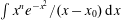
We want to calculate moments in velocity space all the way up to the fourth-order moment
 $r$
, and (including the 3-D geometry) we will need integrals only up to
$r$
, and (including the 3-D geometry) we will need integrals only up to
 $n=5$
. To this aim, we will use frequently (2.49), where we find it convenient to use
$n=5$
. To this aim, we will use frequently (2.49), where we find it convenient to use
 $x_{0}$
and
$x_{0}$
and
 $\unicode[STIX]{x1D701}$
instead of chasing the
$\unicode[STIX]{x1D701}$
instead of chasing the
 $\text{sign}(k_{\Vert })$
, and in the end we will just use the definition
$\text{sign}(k_{\Vert })$
, and in the end we will just use the definition
 $x_{0}=\text{sign}(k_{\Vert })\unicode[STIX]{x1D701}$
. We already saw that the zeroth-order moment was
$x_{0}=\text{sign}(k_{\Vert })\unicode[STIX]{x1D701}$
. We already saw that the zeroth-order moment was
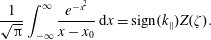 $$\begin{eqnarray}\displaystyle \frac{1}{\sqrt{\unicode[STIX]{x03C0}}}\int _{-\infty }^{\infty }\frac{e^{-x^{2}}}{x-x_{0}}\,\text{d}x=\text{sign}(k_{\Vert })Z(\unicode[STIX]{x1D701}). & & \displaystyle\end{eqnarray}$$
Let us now calculate the higher-order moments. Since we talked so much in the last pages, we will remain silent for a moment and we will just enjoy the calculation,
 $$\begin{eqnarray}\displaystyle \frac{1}{\sqrt{\unicode[STIX]{x03C0}}}\int _{-\infty }^{\infty }\frac{xe^{-x^{2}}}{x-x_{0}}\,\text{d}x & = & \displaystyle \frac{1}{\sqrt{\unicode[STIX]{x03C0}}}\int _{-\infty }^{\infty }\frac{x-x_{0}+x_{0}}{x-x_{0}}e^{-x^{2}}\,\text{d}x\nonumber\\ \displaystyle & = & \displaystyle \underbrace{\frac{1}{\sqrt{\unicode[STIX]{x03C0}}}\int _{-\infty }^{\infty }e^{-x^{2}}\,\text{d}x}_{=1}+\underbrace{\frac{x_{0}}{\sqrt{\unicode[STIX]{x03C0}}}\int _{-\infty }^{\infty }\frac{e^{-x^{2}}}{x-x_{0}}\,\text{d}x}_{=\unicode[STIX]{x1D701}Z(\unicode[STIX]{x1D701})}\nonumber\\ \displaystyle & = & \displaystyle 1+\unicode[STIX]{x1D701}Z(\unicode[STIX]{x1D701})=R(\unicode[STIX]{x1D701}).\end{eqnarray}$$
 $$\begin{eqnarray}\displaystyle \frac{1}{\sqrt{\unicode[STIX]{x03C0}}}\int _{-\infty }^{\infty }\frac{x^{2}e^{-x^{2}}}{x-x_{0}}\,\text{d}x & = & \displaystyle \frac{1}{\sqrt{\unicode[STIX]{x03C0}}}\int _{-\infty }^{\infty }\frac{x^{2}-x_{0}^{2}+x_{0}^{2}}{x-x_{0}}e^{-x^{2}}\,\text{d}x\nonumber\\ \displaystyle & = & \displaystyle \frac{1}{\sqrt{\unicode[STIX]{x03C0}}}\int _{-\infty }^{\infty }(x+x_{0})e^{-x^{2}}\,\text{d}x+\underbrace{\frac{x_{0}^{2}}{\sqrt{\unicode[STIX]{x03C0}}}\int _{-\infty }^{\infty }\frac{e^{-x^{2}}}{x-x_{0}}\,\text{d}x}_{x_{0}\unicode[STIX]{x1D701}Z(\unicode[STIX]{x1D701})}\nonumber\\ \displaystyle & = & \displaystyle \underbrace{\frac{1}{\sqrt{\unicode[STIX]{x03C0}}}\int _{-\infty }^{\infty }xe^{-x^{2}}\,\text{d}x}_{=0}+\underbrace{\frac{x_{0}}{\sqrt{\unicode[STIX]{x03C0}}}\int _{-\infty }^{\infty }e^{-x^{2}}\,\text{d}x}_{=x_{0}}+x_{0}\unicode[STIX]{x1D701}Z(\unicode[STIX]{x1D701})=x_{0}(1+\unicode[STIX]{x1D701}Z(\unicode[STIX]{x1D701}))\nonumber\\ \displaystyle & = & \displaystyle \text{sign}(k_{\Vert })\unicode[STIX]{x1D701}R(\unicode[STIX]{x1D701}).\end{eqnarray}$$
 $$\begin{eqnarray}\displaystyle & \displaystyle \frac{1}{\sqrt{\unicode[STIX]{x03C0}}}\int _{-\infty }^{\infty }\frac{x^{3}e^{-x^{2}}}{x-x_{0}}\,\text{d}x=\underbrace{\frac{1}{\sqrt{\unicode[STIX]{x03C0}}}\int _{-\infty }^{\infty }\frac{x^{3}-x_{0}^{3}}{x-x_{0}}e^{-x^{2}}\,\text{d}x}_{=(1/2)+x_{0}^{2}}+\underbrace{\frac{x_{0}^{3}}{\sqrt{\unicode[STIX]{x03C0}}}\int _{-\infty }^{\infty }\frac{e^{-x^{2}}}{x-x_{0}}\,\text{d}x}_{=\unicode[STIX]{x1D701}^{3}Z(\unicode[STIX]{x1D701})}=\frac{1}{2}+\unicode[STIX]{x1D701}^{2}R(\unicode[STIX]{x1D701}). & \displaystyle \nonumber\\ \displaystyle & & \displaystyle\end{eqnarray}$$
 $$\begin{eqnarray}\displaystyle & \displaystyle \frac{1}{\sqrt{\unicode[STIX]{x03C0}}}\int _{-\infty }^{\infty }\frac{x^{4}e^{-x^{2}}}{x-x_{0}}\,\text{d}x=\text{sign}(k_{\Vert })\left(\frac{1}{2}\unicode[STIX]{x1D701}+\unicode[STIX]{x1D701}^{3}R(\unicode[STIX]{x1D701})\right). & \displaystyle\end{eqnarray}$$
 $$\begin{eqnarray}\displaystyle & \displaystyle \frac{1}{\sqrt{\unicode[STIX]{x03C0}}}\int _{-\infty }^{\infty }\frac{x^{5}e^{-x^{2}}}{x-x_{0}}\,\text{d}x=\frac{3}{4}+\frac{\unicode[STIX]{x1D701}^{2}}{2}+\unicode[STIX]{x1D701}^{4}R(\unicode[STIX]{x1D701}). & \displaystyle\end{eqnarray}$$
That was easy! If we ever need a higher order, we will just blindly calculate
 $$\begin{eqnarray}\displaystyle & & \displaystyle \frac{1}{\sqrt{\unicode[STIX]{x03C0}}}\int _{-\infty }^{\infty }\frac{x^{n}e^{-x^{2}}}{x-x_{0}}\,\text{d}x=\frac{1}{\sqrt{\unicode[STIX]{x03C0}}}\int _{-\infty }^{\infty }\frac{x^{n}-x_{0}^{n}}{x-x_{0}}e^{-x^{2}}\,\text{d}x+\underbrace{\frac{x_{0}^{n}}{\sqrt{\unicode[STIX]{x03C0}}}\int _{-\infty }^{\infty }\frac{e^{-x^{2}}}{x-x_{0}}\,\text{d}x}_{=x_{0}^{n}\text{sign}(k_{\Vert })Z(\unicode[STIX]{x1D701})}\nonumber\\ \displaystyle & & \displaystyle \quad =\frac{1}{\sqrt{\unicode[STIX]{x03C0}}}\int _{-\infty }^{\infty }(x^{n-1}+x^{n-2}x_{0}+x^{n-3}x_{0}^{2}+\cdots +xx_{0}^{n-2}+x_{0}^{n-1})e^{-x^{2}}\,\text{d}x\nonumber\\ \displaystyle & & \displaystyle \qquad +\,\text{sign}(k_{\Vert })^{n+1}\unicode[STIX]{x1D701}^{n}Z(\unicode[STIX]{x1D701}),\end{eqnarray}$$
and we do not worry right now if this general case can be expressed in some smarter way. Now we know how to calculate the kinetic Landau integrals, so let us use this knowledge to calculate the first few integrals of the linear ‘kinetic hierarchy’.
3 One-dimensional geometry (electrostatic)
3.1 Kinetic moments for Maxwellian
$f_{0}$

With the previous integrals already calculated, the calculation of the linear kinetic hierarchy is an easy process. However, it is important to emphasize that the hierarchy is linear, and must be calculated as such. Again, as emphasized before, the kinetic velocity
 $v$
is an independent quantity, and is not linearized. The total density
$v$
is an independent quantity, and is not linearized. The total density
 $n=\int f\,\text{d}v$
, and at the first order of course
$n=\int f\,\text{d}v$
, and at the first order of course
 $n_{0}=\int f_{0}\,\text{d}v$
. The expansion
$n_{0}=\int f_{0}\,\text{d}v$
. The expansion
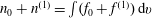 $n_{0}+n^{(1)}=\int (f_{0}+f^{(1)})\,\text{d}v$
implies
$n_{0}+n^{(1)}=\int (f_{0}+f^{(1)})\,\text{d}v$
implies
 $n^{(1)}=\int f^{(1)}\,\text{d}v$
. The density
$n^{(1)}=\int f^{(1)}\,\text{d}v$
. The density
 $n^{(1)}$
, already calculated in (2.50), was therefore calculated correctly, and using the plasma response function
$n^{(1)}$
, already calculated in (2.50), was therefore calculated correctly, and using the plasma response function
 $$\begin{eqnarray}\frac{n^{(1)}}{n_{0}}=-\frac{q_{r}}{T^{(0)}}\unicode[STIX]{x1D6F7}R(\unicode[STIX]{x1D701}).\end{eqnarray}$$
The velocity moment is
 $nu=\int vf\,\text{d}v$
and at the first order
$nu=\int vf\,\text{d}v$
and at the first order
 $n_{0}u_{0}=\int vf_{0}\,\text{d}v$
. In our specific case, because we do not consider any drifts in the distribution function,
$n_{0}u_{0}=\int vf_{0}\,\text{d}v$
. In our specific case, because we do not consider any drifts in the distribution function,
 $u_{0}=0$
. Expanding
$u_{0}=0$
. Expanding
 $(n_{0}+n^{(1)})(u_{0}+u^{(1)})=\int v(f_{0}+f^{(1)})\,\text{d}v$
and neglecting the nonlinear quantity
$(n_{0}+n^{(1)})(u_{0}+u^{(1)})=\int v(f_{0}+f^{(1)})\,\text{d}v$
and neglecting the nonlinear quantity
 $n^{(1)}u^{(1)}$
, yields
$n^{(1)}u^{(1)}$
, yields
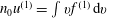 $n_{0}u^{(1)}=\int vf^{(1)}\,\text{d}v$
. The velocity moment calculates as
$n_{0}u^{(1)}=\int vf^{(1)}\,\text{d}v$
. The velocity moment calculates as
 $$\begin{eqnarray}\displaystyle n_{0}u^{(1)} & = & \displaystyle \int vf^{(1)}\,\text{d}v=-\frac{q_{r}}{T^{(0)}}\unicode[STIX]{x1D6F7}\int v\left(1+\frac{{\displaystyle \frac{\unicode[STIX]{x1D714}}{k_{\Vert }}}}{v-{\displaystyle \frac{\unicode[STIX]{x1D714}}{k_{\Vert }}}}\right)f_{0}\,\text{d}v\nonumber\\ \displaystyle & = & \displaystyle -\frac{q_{r}}{T^{(0)}}\unicode[STIX]{x1D6F7}\left(\underbrace{\int vf_{0}\,\text{d}v}_{=n_{0}u_{0}=0}+\int \frac{v{\displaystyle \frac{\unicode[STIX]{x1D714}}{k_{\Vert }}}}{v-{\displaystyle \frac{\unicode[STIX]{x1D714}}{k_{\Vert }}}}f_{0}\,\text{d}v\right)\nonumber\\ \displaystyle & = & \displaystyle -\frac{q_{r}}{T^{(0)}}\unicode[STIX]{x1D6F7}n_{0}\sqrt{\frac{\unicode[STIX]{x1D6FC}}{\unicode[STIX]{x03C0}}}\frac{\unicode[STIX]{x1D714}}{k_{\Vert }}\int \frac{ve^{-\unicode[STIX]{x1D6FC}v^{2}}}{v-{\displaystyle \frac{\unicode[STIX]{x1D714}}{k_{\Vert }}}}\,\text{d}v=\left[\begin{array}{@{}c@{}}\sqrt{\unicode[STIX]{x1D6FC}}v=x\\ \sqrt{\unicode[STIX]{x1D6FC}}\,\text{d}v=\,\text{d}x\end{array}\right]\nonumber\\ \displaystyle & = & \displaystyle -\frac{q_{r}}{T^{(0)}}\unicode[STIX]{x1D6F7}\frac{n_{0}}{\sqrt{\unicode[STIX]{x03C0}}}\frac{\sqrt{\unicode[STIX]{x1D6FC}}}{\sqrt{\unicode[STIX]{x1D6FC}}}\frac{\unicode[STIX]{x1D714}}{k_{\Vert }}\int \frac{xe^{-x^{2}}}{x-{\displaystyle \frac{\unicode[STIX]{x1D714}}{k_{\Vert }}}\sqrt{\unicode[STIX]{x1D6FC}}}\,\text{d}x\nonumber\\ \displaystyle & = & \displaystyle \left[x_{0}=\frac{\unicode[STIX]{x1D714}}{k_{\Vert }}\sqrt{\unicode[STIX]{x1D6FC}}\right]=-\frac{q_{r}}{T^{(0)}}\unicode[STIX]{x1D6F7}\frac{n_{0}}{\sqrt{\unicode[STIX]{x1D6FC}}}\frac{x_{0}}{\sqrt{\unicode[STIX]{x03C0}}}\int _{-\infty }^{\infty }\frac{xe^{-x^{2}}}{x-x_{0}}\,\text{d}x\nonumber\\ \displaystyle & = & \displaystyle -\frac{q_{r}}{T^{(0)}}\unicode[STIX]{x1D6F7}\frac{n_{0}}{\sqrt{\unicode[STIX]{x1D6FC}}}\text{sign}(k_{\Vert })\unicode[STIX]{x1D701}R(\unicode[STIX]{x1D701}),\end{eqnarray}$$
and cancelling
 $n_{0}$
and using
$n_{0}$
and using
 $1/\sqrt{\unicode[STIX]{x1D6FC}}=v_{\text{th}}=\sqrt{2T^{(0)}/m}$
yields
$1/\sqrt{\unicode[STIX]{x1D6FC}}=v_{\text{th}}=\sqrt{2T^{(0)}/m}$
yields
 $$\begin{eqnarray}u^{(1)}=-\frac{q_{r}}{T^{(0)}}\unicode[STIX]{x1D6F7}\sqrt{\frac{2T^{(0)}}{m}}\text{sign}(k_{\Vert })\unicode[STIX]{x1D701}R(\unicode[STIX]{x1D701}).\end{eqnarray}$$
The definition of the scalar pressure is
 $p=m\int (v-u)^{2}f\,\text{d}v$
and at the first order
$p=m\int (v-u)^{2}f\,\text{d}v$
and at the first order
 $p_{0}=m\int v^{2}f_{0}\,\text{d}v$
, because again
$p_{0}=m\int v^{2}f_{0}\,\text{d}v$
, because again
 $u_{0}=0$
. The quantity
$u_{0}=0$
. The quantity
 $(v-u)^{2}=v^{2}-2vu+u^{2}$
is linearized as
$(v-u)^{2}=v^{2}-2vu+u^{2}$
is linearized as
 $v^{2}-2vu^{(1)}$
, and expanding
$v^{2}-2vu^{(1)}$
, and expanding
 $p_{0}+p^{(1)}=m\int (v^{2}-2vu^{(1)})(f_{0}+f^{(1)})\,\text{d}v$
, further linearizing by neglecting
$p_{0}+p^{(1)}=m\int (v^{2}-2vu^{(1)})(f_{0}+f^{(1)})\,\text{d}v$
, further linearizing by neglecting
 $u^{(1)}f^{(1)}$
and using
$u^{(1)}f^{(1)}$
and using
 $u_{0}=0$
yields
$u_{0}=0$
yields
 $p^{(1)}=m\int v^{2}f^{(1)}\,\text{d}v$
. The pressure calculates as
$p^{(1)}=m\int v^{2}f^{(1)}\,\text{d}v$
. The pressure calculates as
 $$\begin{eqnarray}\displaystyle p^{(1)} & = & \displaystyle m\int v^{2}f^{(1)}\,\text{d}v=-\frac{q_{r}}{T^{(0)}}\unicode[STIX]{x1D6F7}\left(\underbrace{m\int v^{2}f_{0}\,\text{d}v}_{=p_{0}}+m\int \frac{v^{2}{\displaystyle \frac{\unicode[STIX]{x1D714}}{k_{\Vert }}}}{v-{\displaystyle \frac{\unicode[STIX]{x1D714}}{k_{\Vert }}}}f_{0}\,\text{d}v\right)=\left[\begin{array}{@{}c@{}}\sqrt{\unicode[STIX]{x1D6FC}}v=x\\ \sqrt{\unicode[STIX]{x1D6FC}}\,\text{d}v=\,\text{d}x\end{array}\right]\nonumber\\ \displaystyle & = & \displaystyle -\frac{q_{r}}{T^{(0)}}\unicode[STIX]{x1D6F7}\left(p_{0}+m\frac{n_{0}}{\sqrt{\unicode[STIX]{x03C0}}}\frac{\sqrt{\unicode[STIX]{x1D6FC}}}{\unicode[STIX]{x1D6FC}}\frac{\unicode[STIX]{x1D714}}{k_{\Vert }}\int \frac{x^{2}e^{-x^{2}}}{x-{\displaystyle \frac{\unicode[STIX]{x1D714}}{k_{\Vert }}}\sqrt{\unicode[STIX]{x1D6FC}}}\,\text{d}x\right)=\left[x_{0}=\frac{\unicode[STIX]{x1D714}}{k_{\Vert }}\sqrt{\unicode[STIX]{x1D6FC}}\right]\nonumber\\ \displaystyle & = & \displaystyle -\frac{q_{r}}{T^{(0)}}\unicode[STIX]{x1D6F7}\left(p_{0}+m\frac{n_{0}}{\unicode[STIX]{x1D6FC}}\frac{x_{0}}{\sqrt{\unicode[STIX]{x03C0}}}\int \frac{x^{2}e^{-x^{2}}}{x-x_{0}}\,\text{d}x\right)=-\frac{q_{r}}{T^{(0)}}\unicode[STIX]{x1D6F7}\left(p_{0}+m\frac{n_{0}}{\unicode[STIX]{x1D6FC}}\unicode[STIX]{x1D701}^{2}R(\unicode[STIX]{x1D701})\right),\end{eqnarray}$$
and dividing by
 $p_{0}$
and using
$p_{0}$
and using
 $p_{0}=n_{0}T^{(0)}$
to calculate
$p_{0}=n_{0}T^{(0)}$
to calculate
 $mn_{0}/(p_{0}\unicode[STIX]{x1D6FC})=2$
, the pressure moment reads
$mn_{0}/(p_{0}\unicode[STIX]{x1D6FC})=2$
, the pressure moment reads
 $$\begin{eqnarray}\frac{p^{(1)}}{p_{0}}=-\frac{q_{r}}{T^{(0)}}\unicode[STIX]{x1D6F7}\left(1+2\unicode[STIX]{x1D701}^{2}R(\unicode[STIX]{x1D701})\right).\end{eqnarray}$$
We will also need the temperature
 $T^{(1)}$
. The general temperature is defined as
$T^{(1)}$
. The general temperature is defined as
 $T=p/n$
, i.e. the definition is nonlinear. The process of linearization is essentially like doing a derivative
$T=p/n$
, i.e. the definition is nonlinear. The process of linearization is essentially like doing a derivative
 $$\begin{eqnarray}\displaystyle T=\frac{p}{n}\overset{\text{lin.}}{\rightarrow }T^{(1)}=\frac{p^{(1)}}{n_{0}}-\frac{p_{0}}{n_{0}^{2}}n^{(1)}, & & \displaystyle\end{eqnarray}$$
and dividing by
 $T^{(0)}=p_{0}/n_{0}$
yields
$T^{(0)}=p_{0}/n_{0}$
yields
 $$\begin{eqnarray}\frac{T^{(1)}}{T^{(0)}}=\frac{p^{(1)}}{p_{0}}-\frac{n^{(1)}}{n_{0}}.\end{eqnarray}$$
If one does not like the ‘derivative’, the same result is obtained by writing
 $p=Tn$
instead, and linearizing
$p=Tn$
instead, and linearizing
 $(p_{0}+p^{(1)})=(T^{(0)}+T^{(1)})(n_{0}+n^{(1)})$
. Which after subtracting
$(p_{0}+p^{(1)})=(T^{(0)}+T^{(1)})(n_{0}+n^{(1)})$
. Which after subtracting
 $p_{0}=T^{(0)}n_{0}$
, neglecting
$p_{0}=T^{(0)}n_{0}$
, neglecting
 $T^{(1)}n^{(1)}$
, yields
$T^{(1)}n^{(1)}$
, yields
 $p^{(1)}=T^{(1)}n_{0}+T^{(0)}n^{(1)}$
, which after dividing by
$p^{(1)}=T^{(1)}n_{0}+T^{(0)}n^{(1)}$
, which after dividing by
 $p_{0}$
yields (3.7). The temperature is therefore easily calculated as
$p_{0}$
yields (3.7). The temperature is therefore easily calculated as
 $$\begin{eqnarray}\frac{T^{(1)}}{T^{(0)}}=-\frac{q_{r}}{T^{(0)}}\unicode[STIX]{x1D6F7}\left(1+2\unicode[STIX]{x1D701}^{2}R(\unicode[STIX]{x1D701})-R(\unicode[STIX]{x1D701})\right).\end{eqnarray}$$
The scalar heat flux is defined as
 $q=m\int (v-u)^{3}f\,\text{d}v$
and at the first order
$q=m\int (v-u)^{3}f\,\text{d}v$
and at the first order
 $q_{0}=m\int v^{3}f_{0}\,\text{d}v$
, and for our case
$q_{0}=m\int v^{3}f_{0}\,\text{d}v$
, and for our case
 $q_{0}=0$
. The quantity
$q_{0}=0$
. The quantity
 $(v-u)^{3}=v^{3}-3v^{2}u+3vu^{2}-u^{3}$
is linearized as
$(v-u)^{3}=v^{3}-3v^{2}u+3vu^{2}-u^{3}$
is linearized as
 $v^{3}-3v^{2}u^{(1)}$
. Expanding
$v^{3}-3v^{2}u^{(1)}$
. Expanding
 $q_{0}+q^{(1)}=m\int (v^{3}-3v^{2}u^{(1)})(f_{0}+f^{(1)})\,\text{d}v$
, neglecting
$q_{0}+q^{(1)}=m\int (v^{3}-3v^{2}u^{(1)})(f_{0}+f^{(1)})\,\text{d}v$
, neglecting
 $u^{(1)}f^{(1)}$
, yields one contribution that is very easy to overlook, and that is of the same order as the expected
$u^{(1)}f^{(1)}$
, yields one contribution that is very easy to overlook, and that is of the same order as the expected
 $m\int v^{3}f^{(1)}\,\text{d}v$
, and that is proportional to
$m\int v^{3}f^{(1)}\,\text{d}v$
, and that is proportional to
 $m\int v^{2}f_{0}\,\text{d}v=p_{0}$
. Therefore, the linearized heat flux
$m\int v^{2}f_{0}\,\text{d}v=p_{0}$
. Therefore, the linearized heat flux
 $q^{(1)}$
must be correctly calculated according to
$q^{(1)}$
must be correctly calculated according to
 $$\begin{eqnarray}q^{(1)}=m\int v^{3}f^{(1)}\,\text{d}v-3p_{0}u^{(1)}.\end{eqnarray}$$
The first term calculates as
 $$\begin{eqnarray}\displaystyle m\int v^{3}f^{(1)}\,\text{d}v & = & \displaystyle -\frac{q_{r}}{T^{(0)}}\unicode[STIX]{x1D6F7}\left(\underbrace{m\int v^{3}f_{0}\,\text{d}v}_{=q_{0}=0}+m\int \frac{v^{3}{\displaystyle \frac{\unicode[STIX]{x1D714}}{k_{\Vert }}}}{v-{\displaystyle \frac{\unicode[STIX]{x1D714}}{k_{\Vert }}}}f_{0}\,\text{d}v\right)=\left[\begin{array}{@{}c@{}}\sqrt{\unicode[STIX]{x1D6FC}}v=x\\ \sqrt{\unicode[STIX]{x1D6FC}}\,\text{d}v=\,\text{d}x\end{array}\right]\nonumber\\ \displaystyle & = & \displaystyle -\frac{q_{r}}{T^{(0)}}\unicode[STIX]{x1D6F7}m\frac{n_{0}}{\sqrt{\unicode[STIX]{x03C0}}}\frac{\sqrt{\unicode[STIX]{x1D6FC}}}{\unicode[STIX]{x1D6FC}^{3/2}}\frac{\unicode[STIX]{x1D714}}{k_{\Vert }}\int \frac{x^{3}e^{-x^{2}}}{x-{\displaystyle \frac{\unicode[STIX]{x1D714}}{k_{\Vert }}}\sqrt{\unicode[STIX]{x1D6FC}}}\,\text{d}x=\left[x_{0}=\frac{\unicode[STIX]{x1D714}}{k_{\Vert }}\sqrt{\unicode[STIX]{x1D6FC}}\right]\nonumber\\ \displaystyle & = & \displaystyle -\frac{q_{r}}{T^{(0)}}\unicode[STIX]{x1D6F7}m\frac{n_{0}}{\unicode[STIX]{x1D6FC}^{3/2}}\frac{x_{0}}{\sqrt{\unicode[STIX]{x03C0}}}\int \frac{x^{3}e^{-x^{2}}}{x-x_{0}}\,\text{d}x\nonumber\\ \displaystyle & = & \displaystyle -q_{r}n_{0}\unicode[STIX]{x1D6F7}\sqrt{\frac{2T^{(0)}}{m}}\text{sign}(k_{\Vert })\left(\unicode[STIX]{x1D701}+2\unicode[STIX]{x1D701}^{3}R(\unicode[STIX]{x1D701})\right),\end{eqnarray}$$
where we used
 $\unicode[STIX]{x1D6FC}^{-3/2}=(2T^{(0)}/m)\sqrt{2T^{(0)}/m}$
. And the entire heat flux (3.9) then reads
$\unicode[STIX]{x1D6FC}^{-3/2}=(2T^{(0)}/m)\sqrt{2T^{(0)}/m}$
. And the entire heat flux (3.9) then reads
 $$\begin{eqnarray}\displaystyle q^{(1)}=-q_{r}n_{0}\unicode[STIX]{x1D6F7}\sqrt{\frac{2T^{(0)}}{m}}\text{sign}(k_{\Vert })\left(\unicode[STIX]{x1D701}+2\unicode[STIX]{x1D701}^{3}R(\unicode[STIX]{x1D701})-3\unicode[STIX]{x1D701}R(\unicode[STIX]{x1D701})\right). & & \displaystyle\end{eqnarray}$$
The scalar fourth-order moment is defined as
 $r=m\int (v-u)^{4}f\,\text{d}v$
and at the first order of course
$r=m\int (v-u)^{4}f\,\text{d}v$
and at the first order of course
 $r_{0}=m\int v^{4}f_{0}\,\text{d}v$
, since again
$r_{0}=m\int v^{4}f_{0}\,\text{d}v$
, since again
 $u_{0}=0$
. Also,
$u_{0}=0$
. Also,
 $r_{0}=3p_{0}^{2}/\unicode[STIX]{x1D70C}_{0}$
, where
$r_{0}=3p_{0}^{2}/\unicode[STIX]{x1D70C}_{0}$
, where
 $\unicode[STIX]{x1D70C}_{0}=mn_{0}$
. The quantity
$\unicode[STIX]{x1D70C}_{0}=mn_{0}$
. The quantity
 $(v-u)^{4}$
is linearized as
$(v-u)^{4}$
is linearized as
 $v^{4}-4v^{3}u^{(1)}$
. Expanding
$v^{4}-4v^{3}u^{(1)}$
. Expanding
 $r_{0}+r^{(1)}=m\int (v^{4}-4v^{3}u^{(1)})(f_{0}+f^{(1)})\,\text{d}v$
, the quantity
$r_{0}+r^{(1)}=m\int (v^{4}-4v^{3}u^{(1)})(f_{0}+f^{(1)})\,\text{d}v$
, the quantity
 $m\int v^{3}f_{0}=q_{0}=0$
, which yields a simple
$m\int v^{3}f_{0}=q_{0}=0$
, which yields a simple
 $r^{(1)}=m\int v^{4}f^{(1)}\,\text{d}v$
. The fourth-order moment calculates as
$r^{(1)}=m\int v^{4}f^{(1)}\,\text{d}v$
. The fourth-order moment calculates as
 $$\begin{eqnarray}\displaystyle r^{(1)} & = & \displaystyle m\int v^{4}f^{(1)}\,\text{d}v=-\frac{q_{r}}{T^{(0)}}\unicode[STIX]{x1D6F7}\left(\underbrace{m\int v^{4}f_{0}\,\text{d}v}_{=r_{0}}+m\int \frac{v^{4}{\displaystyle \frac{\unicode[STIX]{x1D714}}{k_{\Vert }}}}{v-{\displaystyle \frac{\unicode[STIX]{x1D714}}{k_{\Vert }}}}f_{0}\,\text{d}v\right)=\left[\begin{array}{@{}c@{}}\sqrt{\unicode[STIX]{x1D6FC}}v=x\\ \sqrt{\unicode[STIX]{x1D6FC}}\,\text{d}v=\,\text{d}x\end{array}\right]\nonumber\\ \displaystyle & = & \displaystyle -\frac{q_{r}}{T^{(0)}}\unicode[STIX]{x1D6F7}\left(r_{0}+m\frac{n_{0}}{\sqrt{\unicode[STIX]{x03C0}}}\frac{\sqrt{\unicode[STIX]{x1D6FC}}}{\unicode[STIX]{x1D6FC}^{2}}\frac{\unicode[STIX]{x1D714}}{k_{\Vert }}\int \frac{x^{4}e^{-x^{2}}}{x-{\displaystyle \frac{\unicode[STIX]{x1D714}}{k_{\Vert }}}\sqrt{\unicode[STIX]{x1D6FC}}}\,\text{d}x\right)=\left[x_{0}=\frac{\unicode[STIX]{x1D714}}{k_{\Vert }}\sqrt{\unicode[STIX]{x1D6FC}}\right]\nonumber\\ \displaystyle & = & \displaystyle -\frac{q_{r}}{T^{(0)}}\unicode[STIX]{x1D6F7}\left(r_{0}+m\frac{n_{0}}{\unicode[STIX]{x1D6FC}^{2}}\frac{x_{0}}{\sqrt{\unicode[STIX]{x03C0}}}\int \frac{x^{4}e^{-x^{2}}}{x-x_{0}}\,\text{d}x\right)=-\frac{q_{r}p_{0}}{m}\unicode[STIX]{x1D6F7}\left(3+2\unicode[STIX]{x1D701}^{2}+4\unicode[STIX]{x1D701}^{4}R(\unicode[STIX]{x1D701})\right),\nonumber\\ \displaystyle & & \displaystyle\end{eqnarray}$$
where we have used
 $1/\unicode[STIX]{x1D6FC}^{2}=4T^{(0)2}/m^{2}$
, and
$1/\unicode[STIX]{x1D6FC}^{2}=4T^{(0)2}/m^{2}$
, and
 $mn_{0}/\unicode[STIX]{x1D6FC}^{2}=4p_{0}^{2}/\unicode[STIX]{x1D70C}_{0}$
.
$mn_{0}/\unicode[STIX]{x1D6FC}^{2}=4p_{0}^{2}/\unicode[STIX]{x1D70C}_{0}$
.
The entire nonlinear
 $r$
is decomposed as
$r$
is decomposed as
 $r=3p^{2}/\unicode[STIX]{x1D70C}+\widetilde{r}$
. The first term can be linearized in a number of ways, and of course, all techniques must yield the same result, since linearization must be unique. For example, by using the derivative
$r=3p^{2}/\unicode[STIX]{x1D70C}+\widetilde{r}$
. The first term can be linearized in a number of ways, and of course, all techniques must yield the same result, since linearization must be unique. For example, by using the derivative
 $$\begin{eqnarray}\left(\frac{p^{2}}{\unicode[STIX]{x1D70C}}\right)^{\prime }=\frac{1}{\unicode[STIX]{x1D70C}}2pp^{\prime }-\frac{p^{2}}{\unicode[STIX]{x1D70C}^{2}}\unicode[STIX]{x1D70C}^{\prime }=\frac{p^{2}}{\unicode[STIX]{x1D70C}}\left(\frac{2p^{\prime }}{p}-\frac{\unicode[STIX]{x1D70C}^{\prime }}{\unicode[STIX]{x1D70C}}\right),\end{eqnarray}$$
the term is easily linearized as
 $$\begin{eqnarray}\frac{p^{2}}{\unicode[STIX]{x1D70C}}\overset{\text{lin.}}{=}\frac{p_{0}^{2}}{\unicode[STIX]{x1D70C}_{0}}\left(\frac{2p^{(1)}}{p_{0}}-\frac{\unicode[STIX]{x1D70C}^{(1)}}{\unicode[STIX]{x1D70C}_{0}}\right)=\frac{p_{0}^{2}}{\unicode[STIX]{x1D70C}_{0}}\left(\frac{2p^{(1)}}{p_{0}}-\frac{n^{(1)}}{n_{0}}\right),\end{eqnarray}$$
and by further using (3.7), also alternatively as
 $$\begin{eqnarray}\frac{p^{2}}{\unicode[STIX]{x1D70C}}\overset{\text{lin.}}{=}\frac{p_{0}^{2}}{\unicode[STIX]{x1D70C}_{0}}\left(\frac{2T^{(1)}}{T^{(0)}}+\frac{n^{(1)}}{n_{0}}\right).\end{eqnarray}$$
Using
 $r_{0}=3p_{0}^{2}/\unicode[STIX]{x1D70C}_{0}$
therefore yields useful relations (valid for a Maxwellian)
$r_{0}=3p_{0}^{2}/\unicode[STIX]{x1D70C}_{0}$
therefore yields useful relations (valid for a Maxwellian)
 $$\begin{eqnarray}\frac{r^{(1)}}{r_{0}}=2\frac{p^{(1)}}{p_{0}}-\frac{n^{(1)}}{n_{0}}+\frac{\widetilde{r}^{(1)}}{r_{0}}=2\frac{T^{(1)}}{T^{(0)}}+\frac{n^{(1)}}{n_{0}}+\frac{\widetilde{r}^{(1)}}{r_{0}}.\end{eqnarray}$$
Another possibility (to double check the linearization), is to rewrite
 $p^{2}/\unicode[STIX]{x1D70C}=(1/m)pT$
, so that
$p^{2}/\unicode[STIX]{x1D70C}=(1/m)pT$
, so that
 $r=(3/m)pT+\widetilde{r}$
, and to linearize that one instead. Expanding that expression into
$r=(3/m)pT+\widetilde{r}$
, and to linearize that one instead. Expanding that expression into
 $r_{0}+r^{(1)}=(3/m)((p_{0}+p^{(1)})(T^{(0)}+T^{(1)}))+\widetilde{r}^{(1)}$
(where by definition/construction
$r_{0}+r^{(1)}=(3/m)((p_{0}+p^{(1)})(T^{(0)}+T^{(1)}))+\widetilde{r}^{(1)}$
(where by definition/construction
 $\widetilde{r}^{(0)}=0$
), after subtracting
$\widetilde{r}^{(0)}=0$
), after subtracting
 $r_{0}=(3/m)p_{0}T^{(0)}$
, and neglecting
$r_{0}=(3/m)p_{0}T^{(0)}$
, and neglecting
 $p^{(1)}T^{(1)}$
, yields
$p^{(1)}T^{(1)}$
, yields
 $r^{(1)}=(3/m)(p^{(1)}T^{(0)}+p_{0}T^{(1)})+\widetilde{r}^{(1)}$
. Dividing this expression by
$r^{(1)}=(3/m)(p^{(1)}T^{(0)}+p_{0}T^{(1)})+\widetilde{r}^{(1)}$
. Dividing this expression by
 $r_{0}$
yields
$r_{0}$
yields
 $$\begin{eqnarray}\frac{r^{(1)}}{r_{0}}=\frac{p^{(1)}}{p_{0}}+\frac{T^{(1)}}{T^{(0)}}+\frac{\widetilde{r}^{(1)}}{r_{0}},\end{eqnarray}$$
which when used with (3.7), is equivalent to (3.16). Now we can easily calculate the
 $\widetilde{r}^{(1)}$
component as
$\widetilde{r}^{(1)}$
component as
 $$\begin{eqnarray}\widetilde{r}^{(1)}=r^{(1)}-3\frac{p_{0}^{2}}{\unicode[STIX]{x1D70C}_{0}}\left(\frac{2p^{(1)}}{p_{0}}-\frac{n^{(1)}}{n_{0}}\right),\end{eqnarray}$$
that directly yields
 $$\begin{eqnarray}\widetilde{r}^{(1)}=-\frac{q_{r}p_{0}}{m}\unicode[STIX]{x1D6F7}\left(2\unicode[STIX]{x1D701}^{2}+4\unicode[STIX]{x1D701}^{4}R(\unicode[STIX]{x1D701})+3R(\unicode[STIX]{x1D701})-3-12\unicode[STIX]{x1D701}^{2}R(\unicode[STIX]{x1D701})\right).\end{eqnarray}$$
Now we are ready to explore the possible closures.
3.2 Exploring possibilities of a closure
Let us summarize the obtained linear hierarchy so that we can directly see the similarities. Let us also for a moment introduce back the species index
 $r$
, so that we are completely clear
$r$
, so that we are completely clear
 $$\begin{eqnarray}\displaystyle \frac{n_{r}^{(1)}}{n_{0r}} & = & \displaystyle -\frac{q_{r}}{T_{r}^{(0)}}\unicode[STIX]{x1D6F7}R(\unicode[STIX]{x1D701}_{r});\end{eqnarray}$$
 $$\begin{eqnarray}\displaystyle u_{r}^{(1)} & = & \displaystyle -\frac{q_{r}}{T_{r}^{(0)}}\unicode[STIX]{x1D6F7}\sqrt{\frac{2T_{r}^{(0)}}{m_{r}}}\text{sign}(k_{\Vert })\unicode[STIX]{x1D701}_{r}R(\unicode[STIX]{x1D701}_{r});\end{eqnarray}$$
 $$\begin{eqnarray}\displaystyle \frac{p_{r}^{(1)}}{p_{0r}} & = & \displaystyle -\frac{q_{r}}{T_{r}^{(0)}}\unicode[STIX]{x1D6F7}(1+2\unicode[STIX]{x1D701}_{r}^{2}R(\unicode[STIX]{x1D701}_{r}));\end{eqnarray}$$
 $$\begin{eqnarray}\displaystyle \frac{T_{r}^{(1)}}{T_{r}^{(0)}} & = & \displaystyle -\frac{q_{r}}{T_{r}^{(0)}}\unicode[STIX]{x1D6F7}(1+2\unicode[STIX]{x1D701}_{r}^{2}R(\unicode[STIX]{x1D701}_{r})-R(\unicode[STIX]{x1D701}_{r}));\end{eqnarray}$$
 $$\begin{eqnarray}\displaystyle q_{r}^{(1)} & = & \displaystyle -q_{r}n_{0r}\unicode[STIX]{x1D6F7}\sqrt{\frac{2T_{r}^{(0)}}{m_{r}}}\text{sign}(k_{\Vert })(\unicode[STIX]{x1D701}_{r}+2\unicode[STIX]{x1D701}_{r}^{3}R(\unicode[STIX]{x1D701}_{r})-3\unicode[STIX]{x1D701}_{r}R(\unicode[STIX]{x1D701}_{r}));\end{eqnarray}$$
 $$\begin{eqnarray}\displaystyle r_{r}^{(1)} & = & \displaystyle -\frac{q_{r}p_{0r}}{m_{r}}\unicode[STIX]{x1D6F7}(3+2\unicode[STIX]{x1D701}_{r}^{2}+4\unicode[STIX]{x1D701}_{r}^{4}R(\unicode[STIX]{x1D701}_{r}));\end{eqnarray}$$
 $$\begin{eqnarray}\displaystyle \widetilde{r}_{r}^{(1)} & = & \displaystyle -\frac{q_{r}p_{0r}}{m_{r}}\unicode[STIX]{x1D6F7}(2\unicode[STIX]{x1D701}_{r}^{2}+4\unicode[STIX]{x1D701}_{r}^{4}R(\unicode[STIX]{x1D701}_{r})+3R(\unicode[STIX]{x1D701}_{r})-3-12\unicode[STIX]{x1D701}_{r}^{2}R(\unicode[STIX]{x1D701}_{r})),\end{eqnarray}$$
with an emphasis that the charge
 $q_{r}$
should not be confused with the heat flux
$q_{r}$
should not be confused with the heat flux
 $q_{r}^{(1)}$
. The
$q_{r}^{(1)}$
. The
 $\unicode[STIX]{x1D701}_{r}=\unicode[STIX]{x1D714}/(|k_{\Vert }|v_{\text{th}r})$
and the thermal speed
$\unicode[STIX]{x1D701}_{r}=\unicode[STIX]{x1D714}/(|k_{\Vert }|v_{\text{th}r})$
and the thermal speed
 $v_{\text{th}r}=\sqrt{2T_{r}^{(0)}/m_{r}}$
. Note the presence of
$v_{\text{th}r}=\sqrt{2T_{r}^{(0)}/m_{r}}$
. Note the presence of
 $\text{sign}(k_{\Vert })$
in the expressions for
$\text{sign}(k_{\Vert })$
in the expressions for
 $u_{r}^{(1)}$
and
$u_{r}^{(1)}$
and
 $q_{r}^{(1)}$
. The presence of
$q_{r}^{(1)}$
. The presence of
 $\text{sign}(k_{\Vert })$
can be verified a posteriori, for example by considering the simplest situation when the Landau damping is neglected, and the
$\text{sign}(k_{\Vert })$
can be verified a posteriori, for example by considering the simplest situation when the Landau damping is neglected, and the
 $R(\unicode[STIX]{x1D701}_{r})$
function yields only real numbers for real valued
$R(\unicode[STIX]{x1D701}_{r})$
function yields only real numbers for real valued
 $\unicode[STIX]{x1D701}_{r}$
(i.e. the
$\unicode[STIX]{x1D701}_{r}$
(i.e. the
 $R(\unicode[STIX]{x1D701}_{r})$
function can be approximated with Padé approximants that contain only powers of
$R(\unicode[STIX]{x1D701}_{r})$
function can be approximated with Padé approximants that contain only powers of
 $\unicode[STIX]{x1D701}_{r}^{2}$
). Simultaneously changing the signs of
$\unicode[STIX]{x1D701}_{r}^{2}$
). Simultaneously changing the signs of
 $k_{\Vert }$
and
$k_{\Vert }$
and
 $\unicode[STIX]{x1D714}$
in a Fourier mode should give its complex conjugate, i.e. the real part of expressions (3.20)–(3.26) cannot change its sign in that transformation. This is indeed true because the expressions for
$\unicode[STIX]{x1D714}$
in a Fourier mode should give its complex conjugate, i.e. the real part of expressions (3.20)–(3.26) cannot change its sign in that transformation. This is indeed true because the expressions for
 $u_{r}^{(1)}$
and
$u_{r}^{(1)}$
and
 $q_{r}^{(1)}$
contain
$q_{r}^{(1)}$
contain
 $\text{sign}(k_{\Vert })\unicode[STIX]{x1D701}_{r}=\unicode[STIX]{x1D714}/(k_{\Vert }v_{\text{th}r})$
.
$\text{sign}(k_{\Vert })\unicode[STIX]{x1D701}_{r}=\unicode[STIX]{x1D714}/(k_{\Vert }v_{\text{th}r})$
.
To better understand what is meant by ‘a closure’, let us first examine what is not a closure. Let us examine the density
 $n^{(1)}$
equation. Since in this specific example we used the electrostatic electric field
$n^{(1)}$
equation. Since in this specific example we used the electrostatic electric field
 $\boldsymbol{E}^{(1)}=-\unicode[STIX]{x1D735}\unicode[STIX]{x1D719}$
, the only Maxwell equation left is
$\boldsymbol{E}^{(1)}=-\unicode[STIX]{x1D735}\unicode[STIX]{x1D719}$
, the only Maxwell equation left is
 $\unicode[STIX]{x1D735}\boldsymbol{\cdot }\boldsymbol{E}^{(1)}=4\unicode[STIX]{x03C0}\sum _{r}q_{r}n_{r}$
, where
$\unicode[STIX]{x1D735}\boldsymbol{\cdot }\boldsymbol{E}^{(1)}=4\unicode[STIX]{x03C0}\sum _{r}q_{r}n_{r}$
, where
 $q_{r}$
is the charge and
$q_{r}$
is the charge and
 $n_{r}$
is the total density. Linearization of this equation, and using the natural charge neutrality that must be satisfied at the zeroth order
$n_{r}$
is the total density. Linearization of this equation, and using the natural charge neutrality that must be satisfied at the zeroth order
 $\sum _{r}q_{r}n_{0r}=0$
, yields
$\sum _{r}q_{r}n_{0r}=0$
, yields
 $\unicode[STIX]{x1D735}\boldsymbol{\cdot }\boldsymbol{E}^{(1)}=4\unicode[STIX]{x03C0}\sum _{r}q_{r}n_{r}^{(1)}$
, or written with the scalar potential
$\unicode[STIX]{x1D735}\boldsymbol{\cdot }\boldsymbol{E}^{(1)}=4\unicode[STIX]{x03C0}\sum _{r}q_{r}n_{r}^{(1)}$
, or written with the scalar potential
 $-\unicode[STIX]{x1D6FB}^{2}\unicode[STIX]{x1D6F7}=4\unicode[STIX]{x03C0}\sum _{r}q_{r}n_{r}^{(1)}$
, and transformed to Fourier space,
$-\unicode[STIX]{x1D6FB}^{2}\unicode[STIX]{x1D6F7}=4\unicode[STIX]{x03C0}\sum _{r}q_{r}n_{r}^{(1)}$
, and transformed to Fourier space,
 $k^{2}\unicode[STIX]{x1D6F7}=4\unicode[STIX]{x03C0}\sum _{r}q_{r}n_{r}^{(1)}$
. We consider 1-D propagation parallel to
$k^{2}\unicode[STIX]{x1D6F7}=4\unicode[STIX]{x03C0}\sum _{r}q_{r}n_{r}^{(1)}$
. We consider 1-D propagation parallel to
 $\boldsymbol{B}_{0}$
with wavenumber
$\boldsymbol{B}_{0}$
with wavenumber
 $k_{\Vert }$
, and to be consistent, we therefore continue with
$k_{\Vert }$
, and to be consistent, we therefore continue with
 $k_{\Vert }$
and
$k_{\Vert }$
and
 $$\begin{eqnarray}k_{\Vert }^{2}\unicode[STIX]{x1D6F7}=4\unicode[STIX]{x03C0}\mathop{\sum }_{r}q_{r}n_{r}^{(1)}=4\unicode[STIX]{x03C0}\mathop{\sum }_{r}q_{r}n_{0r}\frac{n_{r}^{(1)}}{n_{0r}}=-4\unicode[STIX]{x03C0}\mathop{\sum }_{r}n_{0r}\frac{q_{r}^{2}}{T_{r}^{(0)}}\unicode[STIX]{x1D6F7}R(\unicode[STIX]{x1D701}_{r}),\end{eqnarray}$$
which can be rewritten as
 $$\begin{eqnarray}\left(k_{\Vert }^{2}+4\unicode[STIX]{x03C0}\mathop{\sum }_{r}n_{0r}\frac{q_{r}^{2}}{T_{r}^{(0)}}R(\unicode[STIX]{x1D701}_{r})\right)\unicode[STIX]{x1D6F7}=0.\end{eqnarray}$$
Even though the system is now ‘closed’, the equation (3.28) does not represent a fluid closure, and should be viewed only as a kinetic ‘dispersion relation’. To have a non-trivial solution for the potential
 $\unicode[STIX]{x1D6F7}$
, the expression inside of the bracket must be equal to zero. By declaring that
$\unicode[STIX]{x1D6F7}$
, the expression inside of the bracket must be equal to zero. By declaring that
 $k_{\Vert }\neq 0$
(the case
$k_{\Vert }\neq 0$
(the case
 $k_{\Vert }=0$
is trivial since we need some wavenumber), we can divide by
$k_{\Vert }=0$
is trivial since we need some wavenumber), we can divide by
 $k_{\Vert }^{2}$
. By using the definition of the Debye length of
$k_{\Vert }^{2}$
. By using the definition of the Debye length of
 $r$
-species
$r$
-species
 $\unicode[STIX]{x1D706}_{Dr}=1/k_{Dr}$
, where
$\unicode[STIX]{x1D706}_{Dr}=1/k_{Dr}$
, where
 $k_{Dr}^{2}=4\unicode[STIX]{x03C0}n_{0r}q_{r}^{2}/T_{r}^{(0)}$
, one obtains a dispersion relationFootnote
6
$k_{Dr}^{2}=4\unicode[STIX]{x03C0}n_{0r}q_{r}^{2}/T_{r}^{(0)}$
, one obtains a dispersion relationFootnote
6
 $$\begin{eqnarray}1+\mathop{\sum }_{r}\frac{1}{k_{\Vert }^{2}\unicode[STIX]{x1D706}_{Dr}^{2}}R(\unicode[STIX]{x1D701}_{r})=0.\end{eqnarray}$$
If one replaces here
 $k_{\Vert }\rightarrow k$
, the expression is actually equivalent to a multi-species dispersion relation, usually found in plasma physics books under the electrostatic waves in hot unmagnetized plasmas, with Maxwellian
$k_{\Vert }\rightarrow k$
, the expression is actually equivalent to a multi-species dispersion relation, usually found in plasma physics books under the electrostatic waves in hot unmagnetized plasmas, with Maxwellian
 $f_{0r}$
. See for example Gurnett & Bhattachrjee, page 353, equation (9.4.18). We are not interested here in studying unmagnetized plasmas, and instead, we will just remember (3.29) as the dispersion relation of the parallel propagating (to
$f_{0r}$
. See for example Gurnett & Bhattachrjee, page 353, equation (9.4.18). We are not interested here in studying unmagnetized plasmas, and instead, we will just remember (3.29) as the dispersion relation of the parallel propagating (to
 $\boldsymbol{B}_{0}$
) electrostatic mode in a magnetized plasma, since this mode indeed does not contain any magnetic field fluctuations.
$\boldsymbol{B}_{0}$
) electrostatic mode in a magnetized plasma, since this mode indeed does not contain any magnetic field fluctuations.
Let us consider only the proton and electron species,
 $r=p,e$
, so that
$r=p,e$
, so that
 $$\begin{eqnarray}1+\frac{1}{k_{\Vert }^{2}\unicode[STIX]{x1D706}_{De}^{2}}\left[\frac{T_{e}^{(0)}}{T_{p}^{(0)}}R(\unicode[STIX]{x1D701}_{p})+R(\unicode[STIX]{x1D701}_{e})\right]=0,\end{eqnarray}$$
where the proton Debye length was rewritten with the electron Debye length
 $\unicode[STIX]{x1D706}_{De}=\unicode[STIX]{x1D706}_{Dp}\sqrt{T_{e}^{(0)}/T_{p}^{(0)}}$
. For a general case, the dispersion relation has to be solved numerically, and again, cannot be much simplified, unless one wants to consider the long-wavelength limit
$\unicode[STIX]{x1D706}_{De}=\unicode[STIX]{x1D706}_{Dp}\sqrt{T_{e}^{(0)}/T_{p}^{(0)}}$
. For a general case, the dispersion relation has to be solved numerically, and again, cannot be much simplified, unless one wants to consider the long-wavelength limit
 $k_{\Vert }\unicode[STIX]{x1D706}_{De}\ll 1$
, where only the expression inside of the big brackets can be used. The solution contains the usual Langmuir waves, that are obtained by neglecting the ion term (by making the ions immobile) and by expanding the
$k_{\Vert }\unicode[STIX]{x1D706}_{De}\ll 1$
, where only the expression inside of the big brackets can be used. The solution contains the usual Langmuir waves, that are obtained by neglecting the ion term (by making the ions immobile) and by expanding the
 $R(\unicode[STIX]{x1D701}_{e})$
in the limit
$R(\unicode[STIX]{x1D701}_{e})$
in the limit
 $|\unicode[STIX]{x1D701}_{e}|\gg 1$
, i.e. in the limit when the wave phase speed
$|\unicode[STIX]{x1D701}_{e}|\gg 1$
, i.e. in the limit when the wave phase speed
 $\unicode[STIX]{x1D714}/k$
is much larger than the electron thermal speed
$\unicode[STIX]{x1D714}/k$
is much larger than the electron thermal speed
 $v_{\text{th}e}$
. Langmuir waves propagate with speeds that are higher than the electron plasma frequency
$v_{\text{th}e}$
. Langmuir waves propagate with speeds that are higher than the electron plasma frequency
 $\unicode[STIX]{x1D714}_{pe}=\sqrt{4\unicode[STIX]{x03C0}n_{e0}e^{2}/m_{e}}$
, which for us are extremely high frequencies. The solution also contains the ‘ion-acoustic mode’, which in plasma books is obtained in the limit
$\unicode[STIX]{x1D714}_{pe}=\sqrt{4\unicode[STIX]{x03C0}n_{e0}e^{2}/m_{e}}$
, which for us are extremely high frequencies. The solution also contains the ‘ion-acoustic mode’, which in plasma books is obtained in the limit
 $|\unicode[STIX]{x1D701}_{p}|\gg 1$
and
$|\unicode[STIX]{x1D701}_{p}|\gg 1$
and
 $|\unicode[STIX]{x1D701}_{e}|\ll 1$
, i.e. in the limit where the wave phase speed is much larger than the proton thermal speed,
$|\unicode[STIX]{x1D701}_{e}|\ll 1$
, i.e. in the limit where the wave phase speed is much larger than the proton thermal speed,
 $\unicode[STIX]{x1D714}/k\gg v_{\text{th}p}$
, but also where the phase speed is much smaller than the electron thermal speed,
$\unicode[STIX]{x1D714}/k\gg v_{\text{th}p}$
, but also where the phase speed is much smaller than the electron thermal speed,
 $\unicode[STIX]{x1D714}/k\ll v_{\text{th}e}$
, for the result see for example Gurnett and Bhattacharjee, page 356, equation (9.4.28-29).
$\unicode[STIX]{x1D714}/k\ll v_{\text{th}e}$
, for the result see for example Gurnett and Bhattacharjee, page 356, equation (9.4.28-29).
So what about the limit
 $|\unicode[STIX]{x1D701}_{p}|\ll 1$
, when the phase speed is much smaller than the proton thermal speed
$|\unicode[STIX]{x1D701}_{p}|\ll 1$
, when the phase speed is much smaller than the proton thermal speed
 $\unicode[STIX]{x1D714}/k\ll v_{\text{th}p}$
? Does the ion-acoustic mode not exist in this limit? Unfortunately, in the classical long-wavelength limit, the phase speeds do not become smaller and smaller, the phase speeds
$\unicode[STIX]{x1D714}/k\ll v_{\text{th}p}$
? Does the ion-acoustic mode not exist in this limit? Unfortunately, in the classical long-wavelength limit, the phase speeds do not become smaller and smaller, the phase speeds
 $\unicode[STIX]{x1D714}/k$
just become non-dispersive and constant. In the CGL description (with cold electrons), the parallel propagating ion-acoustic mode has a phase speed
$\unicode[STIX]{x1D714}/k$
just become non-dispersive and constant. In the CGL description (with cold electrons), the parallel propagating ion-acoustic mode has a phase speed
 $\unicode[STIX]{x1D714}/k_{\Vert }=\pm C_{\Vert }$
, where the parallel sound speed
$\unicode[STIX]{x1D714}/k_{\Vert }=\pm C_{\Vert }$
, where the parallel sound speed
 $C_{\Vert }^{2}=3p_{\Vert p}^{(0)}/\unicode[STIX]{x1D70C}_{0}=3T_{\Vert p}^{(0)}/m_{p}$
. The limit
$C_{\Vert }^{2}=3p_{\Vert p}^{(0)}/\unicode[STIX]{x1D70C}_{0}=3T_{\Vert p}^{(0)}/m_{p}$
. The limit
 $|\unicode[STIX]{x1D701}_{p}|\ll 1$
is never satisfied, because
$|\unicode[STIX]{x1D701}_{p}|\ll 1$
is never satisfied, because
 $C_{\Vert }\ll v_{\text{th}\Vert p}$
means
$C_{\Vert }\ll v_{\text{th}\Vert p}$
means
 $\sqrt{3T_{\Vert p}^{(0)}/m_{p}}\ll \sqrt{2T_{\Vert p}^{(0)}/m_{p}}$
, which is never true. One can estimate the lowest possible value of
$\sqrt{3T_{\Vert p}^{(0)}/m_{p}}\ll \sqrt{2T_{\Vert p}^{(0)}/m_{p}}$
, which is never true. One can estimate the lowest possible value of
 $|\unicode[STIX]{x1D701}_{p}|$
to be roughly in the neighbourhood of
$|\unicode[STIX]{x1D701}_{p}|$
to be roughly in the neighbourhood of
 $|\unicode[STIX]{x1D701}_{p}|_{\text{min}}\approx C_{\Vert }^{\text{CGL}}/v_{\text{th}\Vert p}=\sqrt{3/2}$
, or in another words
$|\unicode[STIX]{x1D701}_{p}|_{\text{min}}\approx C_{\Vert }^{\text{CGL}}/v_{\text{th}\Vert p}=\sqrt{3/2}$
, or in another words
 $|\unicode[STIX]{x1D701}_{p}|_{\text{min}}\approx 1$
. There is no expansion of the
$|\unicode[STIX]{x1D701}_{p}|_{\text{min}}\approx 1$
. There is no expansion of the
 $Z(\unicode[STIX]{x1D701})$
for
$Z(\unicode[STIX]{x1D701})$
for
 $|\unicode[STIX]{x1D701}|\approx 1$
and the result has to be found numerically.
$|\unicode[STIX]{x1D701}|\approx 1$
and the result has to be found numerically.
So what constitutes a Landau fluid closure? We will use the following definition: express the last retained moment through lower-order moments in such a way, that the kinetic
 $R(\unicode[STIX]{x1D701})$
function is eliminated (for example by using Padé approximation), so that the closure is expressed only through fluid variables and it is prescribed for all
$R(\unicode[STIX]{x1D701})$
function is eliminated (for example by using Padé approximation), so that the closure is expressed only through fluid variables and it is prescribed for all
 $\unicode[STIX]{x1D701}$
values.
$\unicode[STIX]{x1D701}$
values.
3.2.1 Preliminary closures for
$|\unicode[STIX]{x1D701}|\ll 1$

As explained above, the limit
 $|\unicode[STIX]{x1D701}|\ll 1$
is actually a bit unphysical for the proton species in the electrostatic limit, and is physically plausible only for the electron species. Nevertheless, briefly exploring the linear kinetic hierarchy in this limit allows us to explore what kind of closures might be possible. In this limit, the plasma dispersion function can be expanded as
$|\unicode[STIX]{x1D701}|\ll 1$
is actually a bit unphysical for the proton species in the electrostatic limit, and is physically plausible only for the electron species. Nevertheless, briefly exploring the linear kinetic hierarchy in this limit allows us to explore what kind of closures might be possible. In this limit, the plasma dispersion function can be expanded as
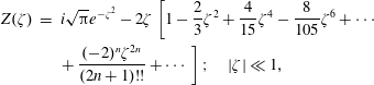 $$\begin{eqnarray}\displaystyle Z(\unicode[STIX]{x1D701}) & = & \displaystyle i\sqrt{\unicode[STIX]{x03C0}}e^{-\unicode[STIX]{x1D701}^{2}}-2\unicode[STIX]{x1D701}\left[1-\frac{2}{3}\unicode[STIX]{x1D701}^{2}+\frac{4}{15}\unicode[STIX]{x1D701}^{4}-\frac{8}{105}\unicode[STIX]{x1D701}^{6}+\cdots \,\right.\nonumber\\ \displaystyle & & \displaystyle \left.+\,\frac{(-2)^{n}\unicode[STIX]{x1D701}^{2n}}{(2n+1)!!}+\cdots \,\right];\quad |\unicode[STIX]{x1D701}|\ll 1,\end{eqnarray}$$
 $$\begin{eqnarray}\displaystyle Z(\unicode[STIX]{x1D701})=i\sqrt{\unicode[STIX]{x03C0}}e^{-\unicode[STIX]{x1D701}^{2}}-2\unicode[STIX]{x1D701}+\frac{4}{3}\unicode[STIX]{x1D701}^{3}-\frac{8}{15}\unicode[STIX]{x1D701}^{5}+\frac{16}{105}\unicode[STIX]{x1D701}^{7}+\cdots \,; & & \displaystyle\end{eqnarray}$$
and the plasma response function as
 $$\begin{eqnarray}\displaystyle R(\unicode[STIX]{x1D701}) & = & \displaystyle 1+i\unicode[STIX]{x1D701}\sqrt{\unicode[STIX]{x03C0}}e^{-\unicode[STIX]{x1D701}^{2}}+\left[-2\unicode[STIX]{x1D701}^{2}+\frac{4}{3}\unicode[STIX]{x1D701}^{4}-\frac{8}{15}\unicode[STIX]{x1D701}^{6}+\frac{16}{105}\unicode[STIX]{x1D701}^{8}+\cdots \,\right.\nonumber\\ \displaystyle & & \displaystyle \left.+\,\frac{(-2)^{n+1}\unicode[STIX]{x1D701}^{2n+2}}{(2n+1)!!}+\cdots \,\right];\quad |\unicode[STIX]{x1D701}|\ll 1,\end{eqnarray}$$
and where for small
 $\unicode[STIX]{x1D701}$
,
$\unicode[STIX]{x1D701}$
,
 $e^{-\unicode[STIX]{x1D701}^{2}}$
is naturally expanded as
$e^{-\unicode[STIX]{x1D701}^{2}}$
is naturally expanded as
 $$\begin{eqnarray}e^{-\unicode[STIX]{x1D701}^{2}}=1-\unicode[STIX]{x1D701}^{2}+\frac{\unicode[STIX]{x1D701}^{4}}{2!}-\frac{\unicode[STIX]{x1D701}^{6}}{3!}+\cdots +\frac{(-1)^{n}\unicode[STIX]{x1D701}^{2n}}{n!}+\cdots \,;\quad |\unicode[STIX]{x1D701}|\ll 1,\end{eqnarray}$$
yielding
 $$\begin{eqnarray}\displaystyle |\unicode[STIX]{x1D701}|\ll 1:\quad Z(\unicode[STIX]{x1D701}) & = & \displaystyle i\sqrt{\unicode[STIX]{x03C0}}-2\unicode[STIX]{x1D701}-i\sqrt{\unicode[STIX]{x03C0}}\unicode[STIX]{x1D701}^{2}+\frac{4}{3}\unicode[STIX]{x1D701}^{3}+i\frac{\sqrt{\unicode[STIX]{x03C0}}}{2}\unicode[STIX]{x1D701}^{4}\nonumber\\ \displaystyle & & \displaystyle -\,\frac{8}{15}\unicode[STIX]{x1D701}^{5}-i\frac{\sqrt{\unicode[STIX]{x03C0}}}{6}\unicode[STIX]{x1D701}^{6}+\frac{16}{105}\unicode[STIX]{x1D701}^{7}+\cdots \,;\end{eqnarray}$$
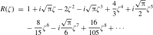 $$\begin{eqnarray}\displaystyle R(\unicode[STIX]{x1D701}) & = & \displaystyle 1+i\sqrt{\unicode[STIX]{x03C0}}\unicode[STIX]{x1D701}-2\unicode[STIX]{x1D701}^{2}-i\sqrt{\unicode[STIX]{x03C0}}\unicode[STIX]{x1D701}^{3}+\frac{4}{3}\unicode[STIX]{x1D701}^{4}+i\frac{\sqrt{\unicode[STIX]{x03C0}}}{2}\unicode[STIX]{x1D701}^{5}\nonumber\\ \displaystyle & & \displaystyle -\,\frac{8}{15}\unicode[STIX]{x1D701}^{6}-i\frac{\sqrt{\unicode[STIX]{x03C0}}}{6}\unicode[STIX]{x1D701}^{7}+\frac{16}{105}\unicode[STIX]{x1D701}^{8}+\cdots\end{eqnarray}$$
For our purposes it is sufficient to keep the series only up to
 $\unicode[STIX]{x1D701}^{3}$
, i.e. to work with the precision
$\unicode[STIX]{x1D701}^{3}$
, i.e. to work with the precision
 $o(\unicode[STIX]{x1D701}^{3})$
. The expressions entering the kinetic hierarchy in (3.20)–(3.26) are
$o(\unicode[STIX]{x1D701}^{3})$
. The expressions entering the kinetic hierarchy in (3.20)–(3.26) are
 $$\begin{eqnarray}\displaystyle R(\unicode[STIX]{x1D701}) & = & \displaystyle 1+i\sqrt{\unicode[STIX]{x03C0}}\unicode[STIX]{x1D701}-2\unicode[STIX]{x1D701}^{2}-i\sqrt{\unicode[STIX]{x03C0}}\unicode[STIX]{x1D701}^{3}+\cdots \,;\quad\end{eqnarray}$$
 $$\begin{eqnarray}\displaystyle \unicode[STIX]{x1D701}R(\unicode[STIX]{x1D701}) & = & \displaystyle \unicode[STIX]{x1D701}+i\sqrt{\unicode[STIX]{x03C0}}\unicode[STIX]{x1D701}^{2}-2\unicode[STIX]{x1D701}^{3};\end{eqnarray}$$
 $$\begin{eqnarray}\displaystyle 1+2\unicode[STIX]{x1D701}^{2}R(\unicode[STIX]{x1D701}) & = & \displaystyle 1+2\unicode[STIX]{x1D701}^{2}+2i\sqrt{\unicode[STIX]{x03C0}}\unicode[STIX]{x1D701}^{3};\end{eqnarray}$$
 $$\begin{eqnarray}\displaystyle 1-R(\unicode[STIX]{x1D701})+2\unicode[STIX]{x1D701}^{2}R(\unicode[STIX]{x1D701}) & = & \displaystyle -i\sqrt{\unicode[STIX]{x03C0}}\unicode[STIX]{x1D701}+4\unicode[STIX]{x1D701}^{2}+3i\sqrt{\unicode[STIX]{x03C0}}\unicode[STIX]{x1D701}^{3};\end{eqnarray}$$
 $$\begin{eqnarray}\displaystyle \unicode[STIX]{x1D701}+2\unicode[STIX]{x1D701}^{3}R(\unicode[STIX]{x1D701})-3\unicode[STIX]{x1D701}R(\unicode[STIX]{x1D701}) & = & \displaystyle -2\unicode[STIX]{x1D701}-3i\sqrt{\unicode[STIX]{x03C0}}\unicode[STIX]{x1D701}^{2}+8\unicode[STIX]{x1D701}^{3};\end{eqnarray}$$
 $$\begin{eqnarray}\displaystyle 3+2\unicode[STIX]{x1D701}^{2}+4\unicode[STIX]{x1D701}^{4}R(\unicode[STIX]{x1D701}) & = & \displaystyle 3+2\unicode[STIX]{x1D701}^{2}+4\unicode[STIX]{x1D701}^{4};\end{eqnarray}$$
 $$\begin{eqnarray}\displaystyle 2\unicode[STIX]{x1D701}^{2}+4\unicode[STIX]{x1D701}^{4}R(\unicode[STIX]{x1D701})+3R(\unicode[STIX]{x1D701})-3-12\unicode[STIX]{x1D701}^{2}R(\unicode[STIX]{x1D701}) & = & \displaystyle 3i\sqrt{\unicode[STIX]{x03C0}}\unicode[STIX]{x1D701}-16\unicode[STIX]{x1D701}^{2}-15i\sqrt{\unicode[STIX]{x03C0}}\unicode[STIX]{x1D701}^{3}.\end{eqnarray}$$
An interesting observation is that for small
 $\unicode[STIX]{x1D701}$
, moments
$\unicode[STIX]{x1D701}$
, moments
 $n^{(1)}$
,
$n^{(1)}$
,
 $p^{(1)}$
and
$p^{(1)}$
and
 $r^{(1)}$
are finite, and moments
$r^{(1)}$
are finite, and moments
 $u^{(1)}$
,
$u^{(1)}$
,
 $T^{(1)}$
,
$T^{(1)}$
,
 $q^{(1)}$
and
$q^{(1)}$
and
 $\widetilde{r}^{(1)}$
are proportional to
$\widetilde{r}^{(1)}$
are proportional to
 $\unicode[STIX]{x1D701}$
and therefore small. We want to make a simple closure for the heat flux
$\unicode[STIX]{x1D701}$
and therefore small. We want to make a simple closure for the heat flux
 $q^{(1)}$
or the fourth-order correction
$q^{(1)}$
or the fourth-order correction
 $\widetilde{r}^{(1)}$
, and thus, let us concentrate on the moments that are small. To clarify how the closure is performed, let us write them down only up to the precision
$\widetilde{r}^{(1)}$
, and thus, let us concentrate on the moments that are small. To clarify how the closure is performed, let us write them down only up to the precision
 $o(\unicode[STIX]{x1D701}_{r}^{2})$
, so
$o(\unicode[STIX]{x1D701}_{r}^{2})$
, so
 $$\begin{eqnarray}\displaystyle u_{r}^{(1)} & = & \displaystyle -\frac{q_{r}}{T_{r}^{(0)}}\unicode[STIX]{x1D6F7}\sqrt{\frac{2T_{r}^{(0)}}{m_{r}}}\text{sign}(k_{\Vert })(\unicode[STIX]{x1D701}_{r}+i\sqrt{\unicode[STIX]{x03C0}}\unicode[STIX]{x1D701}_{r}^{2});\end{eqnarray}$$
 $$\begin{eqnarray}\displaystyle T_{r}^{(1)} & = & \displaystyle -q_{r}\unicode[STIX]{x1D6F7}\left(-i\sqrt{\unicode[STIX]{x03C0}}\unicode[STIX]{x1D701}_{r}+4\unicode[STIX]{x1D701}_{r}^{2}\right);\end{eqnarray}$$
 $$\begin{eqnarray}\displaystyle q_{r}^{(1)} & = & \displaystyle -q_{r}n_{0r}\unicode[STIX]{x1D6F7}\sqrt{\frac{2T_{r}^{(0)}}{m_{r}}}\text{sign}(k_{\Vert })(-2\unicode[STIX]{x1D701}_{r}-3i\sqrt{\unicode[STIX]{x03C0}}\unicode[STIX]{x1D701}_{r}^{2});\end{eqnarray}$$
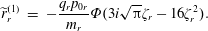 $$\begin{eqnarray}\displaystyle \widetilde{r}_{r}^{(1)} & = & \displaystyle -\frac{q_{r}p_{0r}}{m_{r}}\unicode[STIX]{x1D6F7}(3i\sqrt{\unicode[STIX]{x03C0}}\unicode[STIX]{x1D701}_{r}-16\unicode[STIX]{x1D701}_{r}^{2}).\end{eqnarray}$$
If we further restrict ourselves to only precision
 $o(\unicode[STIX]{x1D701}_{r})$
and neglect the
$o(\unicode[STIX]{x1D701}_{r})$
and neglect the
 $\unicode[STIX]{x1D701}_{r}^{2}$
terms, we can find an amazing result that we can express the heat flux
$\unicode[STIX]{x1D701}_{r}^{2}$
terms, we can find an amazing result that we can express the heat flux
 $q_{r}^{(1)}$
with respect to temperature
$q_{r}^{(1)}$
with respect to temperature
 $T_{r}^{(1)}$
according to
$T_{r}^{(1)}$
according to

The above result is of upmost importance, because it emphasizes the major difference between collisionless and collisional systems. At this point, the result is derived only with the assumption
 $|\unicode[STIX]{x1D701}|\ll 1$
, even though we will see later that the result is not restricted to this limit, and the result has a much wider applicability. The result is the famous expression for collisionless heat flux, that here reads
$|\unicode[STIX]{x1D701}|\ll 1$
, even though we will see later that the result is not restricted to this limit, and the result has a much wider applicability. The result is the famous expression for collisionless heat flux, that here reads
 $q\sim -i\,\text{sign}(k_{\Vert })T$
, which is in strong contrast to the usual collisional heat flux
$q\sim -i\,\text{sign}(k_{\Vert })T$
, which is in strong contrast to the usual collisional heat flux
 $q\sim -\unicode[STIX]{x1D735}_{\Vert }T$
that in Fourier space reads
$q\sim -\unicode[STIX]{x1D735}_{\Vert }T$
that in Fourier space reads
 $q\sim -ik_{\Vert }T$
. We will come to this expression later.
$q\sim -ik_{\Vert }T$
. We will come to this expression later.
With the precision
 $o(\unicode[STIX]{x1D701}_{r})$
, other obvious possibilities are to express
$o(\unicode[STIX]{x1D701}_{r})$
, other obvious possibilities are to express
 $q_{r}^{(1)}$
with respect to velocity
$q_{r}^{(1)}$
with respect to velocity
 $u_{r}^{(1)}$
, or to express
$u_{r}^{(1)}$
, or to express
 $\widetilde{r}^{(1)}$
through
$\widetilde{r}^{(1)}$
through
 $u_{r}^{(1)}$
,
$u_{r}^{(1)}$
,
 $T_{r}^{(1)}$
,
$T_{r}^{(1)}$
,
 $q_{r}^{(1)}$
according to
$q_{r}^{(1)}$
according to
 $$\begin{eqnarray}\displaystyle o(\unicode[STIX]{x1D701}_{r}):\quad q_{r}^{(1)} & = & \displaystyle -2n_{0r}T_{r}^{(0)}u_{r}^{(1)}=-2p_{0r}u_{r}^{(1)};\end{eqnarray}$$
 $$\begin{eqnarray}\displaystyle \widetilde{r}_{r}^{(1)} & = & \displaystyle i{\textstyle \frac{3}{2}}\sqrt{\unicode[STIX]{x03C0}}v_{\text{th}r}p_{0r}\text{sign}(k_{\Vert })u_{r}^{(1)};\end{eqnarray}$$
 $$\begin{eqnarray}\displaystyle \widetilde{r}_{r}^{(1)} & = & \displaystyle -{\textstyle \frac{3}{2}}v_{\text{th}r}^{2}n_{0r}T_{r}^{(1)};\end{eqnarray}$$
 $$\begin{eqnarray}\displaystyle \widetilde{r}_{r}^{(1)} & = & \displaystyle -i{\textstyle \frac{3}{4}}\sqrt{\unicode[STIX]{x03C0}}v_{\text{th}r}\text{sign}(k_{\Vert })q_{r}^{(1)}.\end{eqnarray}$$
However, if we did so much work that we consider the fourth-order moment, it would be a shame not to increase the precision to
 $o(\unicode[STIX]{x1D701}_{r}^{2})$
. Obviously, we need to use a combination of at least 2 different lower-order moments. For example, by trying
$o(\unicode[STIX]{x1D701}_{r}^{2})$
. Obviously, we need to use a combination of at least 2 different lower-order moments. For example, by trying
 $$\begin{eqnarray}o(\unicode[STIX]{x1D701}_{r}^{2}):\quad \widetilde{r}_{r}^{(1)}=\unicode[STIX]{x1D6FC}_{q}q_{r}^{(1)}+\unicode[STIX]{x1D6FC}_{T}T_{r}^{(1)}.\end{eqnarray}$$
The proportionality constants
 $\unicode[STIX]{x1D6FC}_{q}$
,
$\unicode[STIX]{x1D6FC}_{q}$
,
 $\unicode[STIX]{x1D6FC}_{T}$
are easily obtained by separation to two equations for
$\unicode[STIX]{x1D6FC}_{T}$
are easily obtained by separation to two equations for
 $\unicode[STIX]{x1D701}_{r}$
and
$\unicode[STIX]{x1D701}_{r}$
and
 $\unicode[STIX]{x1D701}_{r}^{2}$
that must be satisfied
$\unicode[STIX]{x1D701}_{r}^{2}$
that must be satisfied
 $$\begin{eqnarray}\displaystyle & \displaystyle -\frac{p_{0r}}{m_{r}}3i\sqrt{\unicode[STIX]{x03C0}}=+2\unicode[STIX]{x1D6FC}_{q}n_{0r}v_{\text{th}r}\text{sign}(k_{\Vert })+i\unicode[STIX]{x1D6FC}_{T}\sqrt{\unicode[STIX]{x03C0}}; & \displaystyle\end{eqnarray}$$
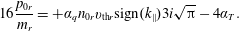 $$\begin{eqnarray}\displaystyle & \displaystyle 16\frac{p_{0r}}{m_{r}}=+\unicode[STIX]{x1D6FC}_{q}n_{0r}v_{\text{th}r}\text{sign}(k_{\Vert })3i\sqrt{\unicode[STIX]{x03C0}}-4\unicode[STIX]{x1D6FC}_{T}. & \displaystyle\end{eqnarray}$$
Playing with the algebra little bit (for example
 $p_{0r}/m_{r}=T_{r}^{(0)}n_{0r}/m_{r}=v_{\text{th}r}^{2}n_{0r}/2$
), the two equations can be solved easily for the unknown quantities
$p_{0r}/m_{r}=T_{r}^{(0)}n_{0r}/m_{r}=v_{\text{th}r}^{2}n_{0r}/2$
), the two equations can be solved easily for the unknown quantities
 $\unicode[STIX]{x1D6FC}_{q}$
,
$\unicode[STIX]{x1D6FC}_{q}$
,
 $\unicode[STIX]{x1D6FC}_{T}$
, and the final result is
$\unicode[STIX]{x1D6FC}_{T}$
, and the final result is
There are naturally other possibilities and with the precision
 $o(\unicode[STIX]{x1D701}_{r}^{2})$
, one can search for closures
$o(\unicode[STIX]{x1D701}_{r}^{2})$
, one can search for closures
 $$\begin{eqnarray}\displaystyle o(\unicode[STIX]{x1D701}_{r}^{2}):\quad q_{r}^{(1)} & = & \displaystyle \unicode[STIX]{x1D6FC}_{T}T_{r}^{(1)}+\unicode[STIX]{x1D6FC}_{u}u_{r}^{(1)};\end{eqnarray}$$
 $$\begin{eqnarray}\displaystyle \widetilde{r}_{r}^{(1)} & = & \displaystyle \unicode[STIX]{x1D6FC}_{q}q_{r}^{(1)}+\unicode[STIX]{x1D6FC}_{u}u_{r}^{(1)};\end{eqnarray}$$
 $$\begin{eqnarray}\displaystyle \widetilde{r}_{r}^{(1)} & = & \displaystyle \unicode[STIX]{x1D6FC}_{T}T_{r}^{(1)}+\unicode[STIX]{x1D6FC}_{u}u_{r}^{(1)},\end{eqnarray}$$
where the first choice yields a closure
and the other two choices yield
 $$\begin{eqnarray}\displaystyle o(\unicode[STIX]{x1D701}_{r}^{2}):\quad \widetilde{r}_{r}^{(1)} & = & \displaystyle -i\frac{16-3\unicode[STIX]{x03C0}}{2\sqrt{\unicode[STIX]{x03C0}}}v_{\text{th}r}\text{sign}(k_{\Vert })q_{r}^{(1)}-i\frac{32-9\unicode[STIX]{x03C0}}{2\sqrt{\unicode[STIX]{x03C0}}}v_{\text{th}r}n_{0r}T_{r}^{(0)}\text{sign}(k_{\Vert })u_{r}^{(1)};\nonumber\\ \displaystyle & & \displaystyle\end{eqnarray}$$
 $$\begin{eqnarray}\displaystyle \widetilde{r}_{r}^{(1)} & = & \displaystyle -\frac{16-3\unicode[STIX]{x03C0}}{8-2\unicode[STIX]{x03C0}}v_{\text{th}r}^{2}n_{0r}T_{r}^{(1)}+i\frac{2\sqrt{\unicode[STIX]{x03C0}}}{\unicode[STIX]{x03C0}-4}v_{\text{th}r}n_{0r}T_{r}^{(0)}\text{sign}(k_{\Vert })u_{r}^{(1)}.\end{eqnarray}$$
For completeness, one can easily find a closure for
 $\widetilde{r}_{r}^{(1)}$
with precision
$\widetilde{r}_{r}^{(1)}$
with precision
 $o(\unicode[STIX]{x1D701}_{r}^{3})$
(after updating (3.44)–(3.47) to precision
$o(\unicode[STIX]{x1D701}_{r}^{3})$
(after updating (3.44)–(3.47) to precision
 $o(\unicode[STIX]{x1D701}_{r}^{3})$
) by searching for a solution
$o(\unicode[STIX]{x1D701}_{r}^{3})$
) by searching for a solution
 $$\begin{eqnarray}o(\unicode[STIX]{x1D701}_{r}^{3}):\quad \widetilde{r}_{r}^{(1)}=\unicode[STIX]{x1D6FC}_{q}q_{r}^{(1)}+\unicode[STIX]{x1D6FC}_{T}T_{r}^{(1)}+\unicode[STIX]{x1D6FC}_{u}u_{r}^{(1)},\end{eqnarray}$$
and the solution reads
We purposely kept the species index
 $r$
in the calculations, to clearly show that the closures are performed for each species separately, and no Maxwell equations or other physical principles are used. The equations would be perhaps easier to read without the index
$r$
in the calculations, to clearly show that the closures are performed for each species separately, and no Maxwell equations or other physical principles are used. The equations would be perhaps easier to read without the index
 $r$
.
$r$
.
3.2.2 Exploring the case
$|\unicode[STIX]{x1D701}|\gg 1$

For large value of
 $|\unicode[STIX]{x1D701}|$
, we need to use an asymptotic expansion of the plasma dispersion function that reads
$|\unicode[STIX]{x1D701}|$
, we need to use an asymptotic expansion of the plasma dispersion function that reads
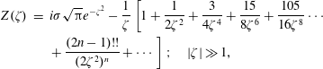 $$\begin{eqnarray}\displaystyle Z(\unicode[STIX]{x1D701}) & = & \displaystyle i\unicode[STIX]{x1D70E}\sqrt{\unicode[STIX]{x03C0}}e^{-\unicode[STIX]{x1D701}^{2}}-\frac{1}{\unicode[STIX]{x1D701}}\left[1+\frac{1}{2\unicode[STIX]{x1D701}^{2}}+\frac{3}{4\unicode[STIX]{x1D701}^{4}}+\frac{15}{8\unicode[STIX]{x1D701}^{6}}+\frac{105}{16\unicode[STIX]{x1D701}^{8}}\cdots \,\right.\nonumber\\ \displaystyle & & \displaystyle \left.+\,\frac{(2n-1)!!}{(2\unicode[STIX]{x1D701}^{2})^{n}}+\cdots \,\right];\quad |\unicode[STIX]{x1D701}|\gg 1,\end{eqnarray}$$
where
 $$\begin{eqnarray}\unicode[STIX]{x1D70E}=\left\{\begin{array}{@{}ll@{}}0,\quad & \text{Im}(\unicode[STIX]{x1D701})>0;\\ 1,\quad & \text{Im}(\unicode[STIX]{x1D701})=0;\\ 2,\quad & \text{Im}(\unicode[STIX]{x1D701})<0.\end{array}\right.\end{eqnarray}$$
The term with
 $\unicode[STIX]{x1D70E}$
comes directly from the definition of
$\unicode[STIX]{x1D70E}$
comes directly from the definition of
 $Z(\unicode[STIX]{x1D701})$
and there is not much one can do further about it, since there is no further asymptotic expansion for
$Z(\unicode[STIX]{x1D701})$
and there is not much one can do further about it, since there is no further asymptotic expansion for
 $\exp (-\unicode[STIX]{x1D701}^{2})$
when
$\exp (-\unicode[STIX]{x1D701}^{2})$
when
 $\unicode[STIX]{x1D701}$
is large. The term is zero in the upper half of complex plane (
$\unicode[STIX]{x1D701}$
is large. The term is zero in the upper half of complex plane (
 $\unicode[STIX]{x1D70E}=0$
). When very close to the real axis, i.e. when
$\unicode[STIX]{x1D70E}=0$
). When very close to the real axis, i.e. when
 $\unicode[STIX]{x1D70E}=1$
, the term mainly contributes to the imaginary part of
$\unicode[STIX]{x1D70E}=1$
, the term mainly contributes to the imaginary part of
 $Z(\unicode[STIX]{x1D701})$
(even though only very weakly) and for the real part of
$Z(\unicode[STIX]{x1D701})$
(even though only very weakly) and for the real part of
 $Z(\unicode[STIX]{x1D701})$
, its contribution can be neglected. However, when deeply down in the lower half of complex plane, the term can become very large (for example if
$Z(\unicode[STIX]{x1D701})$
, its contribution can be neglected. However, when deeply down in the lower half of complex plane, the term can become very large (for example if
 $\unicode[STIX]{x1D701}=-iy$
,
$\unicode[STIX]{x1D701}=-iy$
,
 $\exp (-\unicode[STIX]{x1D701}^{2})=\exp (y^{2})$
and if
$\exp (-\unicode[STIX]{x1D701}^{2})=\exp (y^{2})$
and if
 $y$
is large the term obviously explodes). Deeply down in the lower complex plane the term is a real trouble, and even some kinetic solvers such as WHAMP (Rönnmark Reference Rönnmark1982) have trouble with calculations when the damping is too large.
$y$
is large the term obviously explodes). Deeply down in the lower complex plane the term is a real trouble, and even some kinetic solvers such as WHAMP (Rönnmark Reference Rönnmark1982) have trouble with calculations when the damping is too large.
We will see shortly, that for our purposes the term can be completely neglected, but let us keep it for a moment. The expansion of the Maxwellian plasma response function therefore reads
 $$\begin{eqnarray}R(\unicode[STIX]{x1D701})=i\unicode[STIX]{x1D70E}\sqrt{\unicode[STIX]{x03C0}}\unicode[STIX]{x1D701}e^{-\unicode[STIX]{x1D701}^{2}}-\frac{1}{2\unicode[STIX]{x1D701}^{2}}-\frac{3}{4\unicode[STIX]{x1D701}^{4}}-\frac{15}{8\unicode[STIX]{x1D701}^{6}}-\frac{105}{16\unicode[STIX]{x1D701}^{8}}-\frac{945}{32\unicode[STIX]{x1D701}^{10}}\cdots \,;\quad |\unicode[STIX]{x1D701}|\gg 1.\end{eqnarray}$$
Let us calculate the kinetic hierarchy, at least up to
 $1/\unicode[STIX]{x1D701}^{4}$
. After a short inspection, one immediately sees that the hierarchy calculates a bit differently than in the previous case, and to get the fourth-order moments with the precision
$1/\unicode[STIX]{x1D701}^{4}$
. After a short inspection, one immediately sees that the hierarchy calculates a bit differently than in the previous case, and to get the fourth-order moments with the precision
 $o(1/\unicode[STIX]{x1D701}^{4})$
, it is important to keep all the terms up to
$o(1/\unicode[STIX]{x1D701}^{4})$
, it is important to keep all the terms up to
 ${\sim}1/\unicode[STIX]{x1D701}^{8}$
in the
${\sim}1/\unicode[STIX]{x1D701}^{8}$
in the
 $R(\unicode[STIX]{x1D701})$
expression, since the fourth-order moments contain
$R(\unicode[STIX]{x1D701})$
expression, since the fourth-order moments contain
 $\unicode[STIX]{x1D701}^{4}R(\unicode[STIX]{x1D701})$
terms. The expressions entering the kinetic hierarchy dully calculate as
$\unicode[STIX]{x1D701}^{4}R(\unicode[STIX]{x1D701})$
terms. The expressions entering the kinetic hierarchy dully calculate as
 $$\begin{eqnarray}\displaystyle & \displaystyle n^{(1)}\sim R(\unicode[STIX]{x1D701})=i\unicode[STIX]{x1D70E}\sqrt{\unicode[STIX]{x03C0}}\unicode[STIX]{x1D701}e^{-\unicode[STIX]{x1D701}^{2}}-\frac{1}{2\unicode[STIX]{x1D701}^{2}}-\frac{3}{4\unicode[STIX]{x1D701}^{4}}+o\left(\frac{1}{\unicode[STIX]{x1D701}^{4}}\right); & \displaystyle\end{eqnarray}$$
 $$\begin{eqnarray}\displaystyle & \displaystyle u^{(1)}\sim \unicode[STIX]{x1D701}R(\unicode[STIX]{x1D701})=i\unicode[STIX]{x1D70E}\sqrt{\unicode[STIX]{x03C0}}\unicode[STIX]{x1D701}^{2}e^{-\unicode[STIX]{x1D701}^{2}}-\frac{1}{2\unicode[STIX]{x1D701}}-\frac{3}{4\unicode[STIX]{x1D701}^{3}}-\frac{15}{8\unicode[STIX]{x1D701}^{5}}; & \displaystyle\end{eqnarray}$$
 $$\begin{eqnarray}\displaystyle & \displaystyle p^{(1)}\sim 1+2\unicode[STIX]{x1D701}^{2}R(\unicode[STIX]{x1D701})=2i\unicode[STIX]{x1D70E}\sqrt{\unicode[STIX]{x03C0}}\unicode[STIX]{x1D701}^{3}e^{-\unicode[STIX]{x1D701}^{2}}-\frac{3}{2\unicode[STIX]{x1D701}^{2}}-\frac{15}{4\unicode[STIX]{x1D701}^{4}}; & \displaystyle\end{eqnarray}$$
 $$\begin{eqnarray}\displaystyle & \displaystyle T^{(1)}\sim 1-R(\unicode[STIX]{x1D701})+2\unicode[STIX]{x1D701}^{2}R(\unicode[STIX]{x1D701})=i\unicode[STIX]{x1D70E}\sqrt{\unicode[STIX]{x03C0}}e^{-\unicode[STIX]{x1D701}^{2}}(2\unicode[STIX]{x1D701}^{3}-\unicode[STIX]{x1D701})-\frac{1}{\unicode[STIX]{x1D701}^{2}}-\frac{3}{\unicode[STIX]{x1D701}^{4}}; & \displaystyle\end{eqnarray}$$
 $$\begin{eqnarray}\displaystyle & \displaystyle q^{(1)}\sim \unicode[STIX]{x1D701}+2\unicode[STIX]{x1D701}^{3}R(\unicode[STIX]{x1D701})-3\unicode[STIX]{x1D701}R(\unicode[STIX]{x1D701})=i\unicode[STIX]{x1D70E}\sqrt{\unicode[STIX]{x03C0}}e^{-\unicode[STIX]{x1D701}^{2}}(2\unicode[STIX]{x1D701}^{4}-3\unicode[STIX]{x1D701}^{2})-\frac{3}{2\unicode[STIX]{x1D701}^{3}}-\frac{15}{2\unicode[STIX]{x1D701}^{5}}; & \displaystyle\end{eqnarray}$$
 $$\begin{eqnarray}\displaystyle & \displaystyle r^{(1)}\sim 3+2\unicode[STIX]{x1D701}^{2}+4\unicode[STIX]{x1D701}^{4}R(\unicode[STIX]{x1D701})=4i\unicode[STIX]{x1D70E}\sqrt{\unicode[STIX]{x03C0}}\unicode[STIX]{x1D701}^{5}e^{-\unicode[STIX]{x1D701}^{2}}-\frac{15}{2\unicode[STIX]{x1D701}^{2}}-\frac{105}{4\unicode[STIX]{x1D701}^{4}}; & \displaystyle\end{eqnarray}$$
 $$\begin{eqnarray}\widetilde{r}^{(1)}\sim 2\unicode[STIX]{x1D701}^{2}+4\unicode[STIX]{x1D701}^{4}R(\unicode[STIX]{x1D701})+3R(\unicode[STIX]{x1D701})-3-12\unicode[STIX]{x1D701}^{2}R(\unicode[STIX]{x1D701})=i\unicode[STIX]{x1D70E}\sqrt{\unicode[STIX]{x03C0}}e^{-\unicode[STIX]{x1D701}^{2}}(4\unicode[STIX]{x1D701}^{5}-12\unicode[STIX]{x1D701}^{3}+3\unicode[STIX]{x1D701})-\frac{6}{\unicode[STIX]{x1D701}^{4}},\end{eqnarray}$$
where for brevity we suppressed the proportionality constants, including the
 $\text{sign}(k_{\Vert })$
. Interestingly, the velocity
$\text{sign}(k_{\Vert })$
. Interestingly, the velocity
 $u^{(1)}$
decreases the slowest, only as
$u^{(1)}$
decreases the slowest, only as
 $1/\unicode[STIX]{x1D701}$
. The
$1/\unicode[STIX]{x1D701}$
. The
 $n^{(1)}$
,
$n^{(1)}$
,
 $p^{(1)}$
,
$p^{(1)}$
,
 $r^{(1)}$
and also the temperature
$r^{(1)}$
and also the temperature
 $T^{(1)}$
, decrease as
$T^{(1)}$
, decrease as
 $1/\unicode[STIX]{x1D701}^{2}$
. The heat flux
$1/\unicode[STIX]{x1D701}^{2}$
. The heat flux
 $q^{(1)}$
decreases as
$q^{(1)}$
decreases as
 $1/\unicode[STIX]{x1D701}^{3}$
and the cumulant
$1/\unicode[STIX]{x1D701}^{3}$
and the cumulant
 $\widetilde{r}^{(1)}$
decreases the fastest, as
$\widetilde{r}^{(1)}$
decreases the fastest, as
 $1/\unicode[STIX]{x1D701}^{4}$
. This is not good news, since it is obvious that the direct closures that were easily obtained for the small
$1/\unicode[STIX]{x1D701}^{4}$
. This is not good news, since it is obvious that the direct closures that were easily obtained for the small
 $\unicode[STIX]{x1D701}$
case, cannot be easily done here.
$\unicode[STIX]{x1D701}$
case, cannot be easily done here.
To understand how the terms contribute to the real frequency and damping, it is useful to separate
 $\unicode[STIX]{x1D701}=x+iy$
and calculate expressions with
$\unicode[STIX]{x1D701}=x+iy$
and calculate expressions with
 $y$
being small, i.e. the weak growth-rate (actually weak damping) approximation. The exponential term entering (3.67) can be approximated as
$y$
being small, i.e. the weak growth-rate (actually weak damping) approximation. The exponential term entering (3.67) can be approximated as
 $$\begin{eqnarray}\displaystyle \unicode[STIX]{x1D701}^{2} & = & \displaystyle (x+iy)^{2}=(x^{2}-y^{2})+2ixy\approx x^{2}+2ixy;\nonumber\\ \displaystyle e^{-\unicode[STIX]{x1D701}^{2}} & {\approx} & \displaystyle e^{-x^{2}}e^{-2ixy};\nonumber\\ \displaystyle i\unicode[STIX]{x1D701}e^{-\unicode[STIX]{x1D701}^{2}} & = & \displaystyle i(x+iy)e^{-(x+iy)^{2}}\approx (-y+ix)e^{-x^{2}}e^{-2ixy},\end{eqnarray}$$
and the fractions of
 $\unicode[STIX]{x1D701}$
are approximately
$\unicode[STIX]{x1D701}$
are approximately
 $$\begin{eqnarray}\displaystyle & \displaystyle \frac{1}{\unicode[STIX]{x1D701}}=\frac{1}{x+iy}=\frac{1}{x\left(1+i{\displaystyle \frac{y}{x}}\right)}\approx \frac{1}{x}\left(1-i\frac{y}{x}\right)=\frac{1}{x}-i\frac{y}{x^{2}}; & \displaystyle\end{eqnarray}$$
 $$\begin{eqnarray}\displaystyle & \displaystyle \frac{1}{\unicode[STIX]{x1D701}^{2}}=\frac{1}{x^{2}\left(1+i{\displaystyle \frac{y}{x}}\right)^{2}}\approx \frac{1}{x^{2}}\left(1-2i\frac{y}{x}\right)=\frac{1}{x^{2}}-2i\frac{y}{x^{3}}; & \displaystyle\end{eqnarray}$$
 $$\begin{eqnarray}\displaystyle & \displaystyle \frac{1}{\unicode[STIX]{x1D701}^{3}}\approx \frac{1}{x^{3}}-3i\frac{y}{x^{4}}; & \displaystyle\end{eqnarray}$$
 $$\begin{eqnarray}\displaystyle & \displaystyle \frac{1}{\unicode[STIX]{x1D701}^{4}}\approx \frac{1}{x^{4}}-4i\frac{y}{x^{5}}, & \displaystyle\end{eqnarray}$$
etc. For large
 $x$
, the exponential term (3.75) is strongly suppressed as
$x$
, the exponential term (3.75) is strongly suppressed as
 $e^{-x^{2}}$
(with oscillations
$e^{-x^{2}}$
(with oscillations
 $e^{i2xy}$
). Additionally, the real part of (3.75) is proportional to
$e^{i2xy}$
). Additionally, the real part of (3.75) is proportional to
 $y$
, which is also small, and its contribution to the real part of
$y$
, which is also small, and its contribution to the real part of
 $R(\unicode[STIX]{x1D701})$
can be therefore completely neglected. The imaginary part of the exponential term (3.75) has to be kept, if one wants to match the approximate kinetic dispersion relations from plasma books (usually calculated in the weak growth rate/damping approximation), for example for the damping of the Langmuir mode or the ion-acoustic mode. However, even smart plasma physics books have trouble analytically reproducing the full kinetic dispersion relations that have to be solved numerically, see for example figures in Gurnett and Bhattacharjee on pages 341 and 355, that compare the analytic and full solutions for the Langmuir mode and the ion-acoustic mode. The trouble is that the damping can become large, and the entire approach with the weak damping invalid. If kinetic plasma books have trouble analytically reproducing the damping with full accuracy under these conditions, we would be naive to think that we can do better with a fluid model and we know we cannot be analytically exact for
$R(\unicode[STIX]{x1D701})$
can be therefore completely neglected. The imaginary part of the exponential term (3.75) has to be kept, if one wants to match the approximate kinetic dispersion relations from plasma books (usually calculated in the weak growth rate/damping approximation), for example for the damping of the Langmuir mode or the ion-acoustic mode. However, even smart plasma physics books have trouble analytically reproducing the full kinetic dispersion relations that have to be solved numerically, see for example figures in Gurnett and Bhattacharjee on pages 341 and 355, that compare the analytic and full solutions for the Langmuir mode and the ion-acoustic mode. The trouble is that the damping can become large, and the entire approach with the weak damping invalid. If kinetic plasma books have trouble analytically reproducing the damping with full accuracy under these conditions, we would be naive to think that we can do better with a fluid model and we know we cannot be analytically exact for
 $|\unicode[STIX]{x1D701}|\gg 1$
if the damping is too large. If the damping is far too large, and the imaginary frequency starts to be comparable to real frequency, the mode will be damped away very quickly.
$|\unicode[STIX]{x1D701}|\gg 1$
if the damping is too large. If the damping is far too large, and the imaginary frequency starts to be comparable to real frequency, the mode will be damped away very quickly.
In fact, even the well-known kinetic solver WHAMP, neglects this term in calculation of
 $Z(\unicode[STIX]{x1D701})$
for large
$Z(\unicode[STIX]{x1D701})$
for large
 $\unicode[STIX]{x1D701}$
values, as can be verified in the WHAMP full manual (Rönnmark Reference Rönnmark1982) from the asymptotic expansion of
$\unicode[STIX]{x1D701}$
values, as can be verified in the WHAMP full manual (Rönnmark Reference Rönnmark1982) from the asymptotic expansion of
 $Z(\unicode[STIX]{x1D701})$
, equation (III-6) on page 10, and the discussion of numerical errors on page 13. The WHAMP solver uses an eight-pole Padé approximant of
$Z(\unicode[STIX]{x1D701})$
, equation (III-6) on page 10, and the discussion of numerical errors on page 13. The WHAMP solver uses an eight-pole Padé approximant of
 $Z(\unicode[STIX]{x1D701})$
, which is a very precise approximant, and imprecision starts to show up only if the damping become too large. For example, in the very damped regime when the
$Z(\unicode[STIX]{x1D701})$
, which is a very precise approximant, and imprecision starts to show up only if the damping become too large. For example, in the very damped regime when the
 $\text{Im}(\unicode[STIX]{x1D701})=-\text{Re}(\unicode[STIX]{x1D701})/2$
, the error in real and imaginary values of
$\text{Im}(\unicode[STIX]{x1D701})=-\text{Re}(\unicode[STIX]{x1D701})/2$
, the error in real and imaginary values of
 $Z(\unicode[STIX]{x1D701})$
is still less than 2 %–3 %, where the calculation should be stopped (in a less damped regime, the precision is much higher).
$Z(\unicode[STIX]{x1D701})$
is still less than 2 %–3 %, where the calculation should be stopped (in a less damped regime, the precision is much higher).
If a full kinetic solver can neglect the exponential term for large
 $\unicode[STIX]{x1D701}$
values, we can surely neglect it as well. It should be emphasized that the term is neglected only for large
$\unicode[STIX]{x1D701}$
values, we can surely neglect it as well. It should be emphasized that the term is neglected only for large
 $\unicode[STIX]{x1D701}$
values (i.e. in the asymptotic expansion), the exponential term is otherwise fully retained and enters the Padé approximation through the power series expansion for small
$\unicode[STIX]{x1D701}$
values (i.e. in the asymptotic expansion), the exponential term is otherwise fully retained and enters the Padé approximation through the power series expansion for small
 $\unicode[STIX]{x1D701}$
. To summarize, the ‘ideal’ large
$\unicode[STIX]{x1D701}$
. To summarize, the ‘ideal’ large
 $\unicode[STIX]{x1D701}$
asymptotic behaviour that we would like to obtain reads
$\unicode[STIX]{x1D701}$
asymptotic behaviour that we would like to obtain reads
 $$\begin{eqnarray}\displaystyle \frac{n_{r}^{(1)}}{n_{0r}} & = & \displaystyle -\frac{q_{r}}{T_{r}^{(0)}}\unicode[STIX]{x1D6F7}\left[-\frac{1}{2\unicode[STIX]{x1D701}^{2}}-\frac{3}{4\unicode[STIX]{x1D701}^{4}}-\cdots \,\right];\end{eqnarray}$$
 $$\begin{eqnarray}\displaystyle u_{r}^{(1)} & = & \displaystyle -\frac{q_{r}}{T_{r}^{(0)}}\unicode[STIX]{x1D6F7}v_{\text{th}r}\text{sign}(k_{\Vert })\left[-\frac{1}{2\unicode[STIX]{x1D701}}-\frac{3}{4\unicode[STIX]{x1D701}^{3}}-\cdots \,\right];\end{eqnarray}$$
 $$\begin{eqnarray}\displaystyle \frac{p_{r}^{(1)}}{p_{0r}} & = & \displaystyle -\frac{q_{r}}{T_{r}^{(0)}}\unicode[STIX]{x1D6F7}\left[-\frac{3}{2\unicode[STIX]{x1D701}^{2}}-\frac{15}{4\unicode[STIX]{x1D701}^{4}}-\cdots \,\right];\end{eqnarray}$$
 $$\begin{eqnarray}\displaystyle \frac{T_{r}^{(1)}}{T_{r}^{(0)}} & = & \displaystyle -\frac{q_{r}}{T_{r}^{(0)}}\unicode[STIX]{x1D6F7}\left[-\frac{1}{\unicode[STIX]{x1D701}^{2}}-\frac{3}{\unicode[STIX]{x1D701}^{4}}-\cdots \,\right];\end{eqnarray}$$
 $$\begin{eqnarray}\displaystyle q_{r}^{(1)} & = & \displaystyle -q_{r}n_{0r}\unicode[STIX]{x1D6F7}v_{\text{th}r}\text{sign}(k_{\Vert })\left[-\frac{3}{2\unicode[STIX]{x1D701}^{3}}-\frac{15}{2\unicode[STIX]{x1D701}^{5}}-\cdots \,\right];\end{eqnarray}$$
 $$\begin{eqnarray}\displaystyle r_{r}^{(1)} & = & \displaystyle -\frac{q_{r}p_{0r}}{m_{r}}\unicode[STIX]{x1D6F7}\left[-\frac{15}{2\unicode[STIX]{x1D701}^{2}}-\frac{105}{4\unicode[STIX]{x1D701}^{4}}-\cdots \,\right];\end{eqnarray}$$
 $$\begin{eqnarray}\displaystyle \widetilde{r}_{r}^{(1)} & = & \displaystyle -\frac{q_{r}p_{0r}}{m_{r}}\unicode[STIX]{x1D6F7}\left[-\frac{6}{\unicode[STIX]{x1D701}^{4}}-\cdots \,\right].\end{eqnarray}$$
3.3 A brief introduction to Padé approximants
Padé approximants, i.e. Padé series approximation/expansion, is a very powerful mathematical technique, comparable to the usual Taylor series and the Laurent series. Nevertheless, for some unknown reason, Padé series seems to somehow disappear from the modern educational system that a typical physicist encounters. The lack of Padé series in classes is even more surprising, if one realizes that the technique is in fact very simple, and anybody can fully grasp it in very short time. We therefore make a quick introduction to the technique here.
Padé series consist of approximating a function as a ratio of two polynomials. If a power series (e.g. Taylor series) of a function
 $f(x)$
is known around some point with coefficients
$f(x)$
is known around some point with coefficients
 $c_{n}$
, the goal is to express it as a ratio of two polynomials
$c_{n}$
, the goal is to express it as a ratio of two polynomials
 $$\begin{eqnarray}c_{0}+c_{1}x+c_{2}x^{2}+c_{3}x^{3}+c_{4}x^{4}+\cdots =\frac{a_{0}+a_{1}x+a_{2}x^{2}+\cdots }{1+b_{1}x+b_{2}x^{2}+\cdots }\end{eqnarray}$$
The choice of
 $b_{0}=1$
is an ad hoc choice and the entire decomposition can be done without it, leading to the same results at the end. Multiplying the left-hand side by the denominator
$b_{0}=1$
is an ad hoc choice and the entire decomposition can be done without it, leading to the same results at the end. Multiplying the left-hand side by the denominator
 $1+b_{1}x+b_{2}x^{2}+\cdots \,$
, and grouping the
$1+b_{1}x+b_{2}x^{2}+\cdots \,$
, and grouping the
 $x^{n}$
contributions together, that must be satisfied independently, leads to the system of equations
$x^{n}$
contributions together, that must be satisfied independently, leads to the system of equations
 $$\begin{eqnarray}\displaystyle a_{0} & = & \displaystyle c_{0};\nonumber\\ \displaystyle a_{1} & = & \displaystyle c_{1}+c_{0}b_{1};\nonumber\\ \displaystyle a_{2} & = & \displaystyle c_{2}+c_{1}b_{1}+c_{0}b_{2};\nonumber\\ \displaystyle a_{3} & = & \displaystyle c_{3}+c_{2}b_{1}+c_{1}b_{2}+c_{0}b_{3};\nonumber\\ \displaystyle a_{4} & = & \displaystyle c_{4}+c_{3}b_{1}+c_{2}b_{2}+c_{1}b_{3}+c_{0}b_{4};\nonumber\\ \displaystyle a_{5} & = & \displaystyle c_{5}+c_{4}b_{1}+c_{3}b_{2}+c_{2}b_{3}+c_{1}b_{4}+c_{0}b_{5};\nonumber\\ \displaystyle a_{6} & = & \displaystyle c_{6}+c_{5}b_{1}+c_{4}b_{2}+c_{3}b_{3}+c_{2}b_{4}+c_{1}b_{5}+c_{0}b_{6},\end{eqnarray}$$
etc. The necessary condition for the system being solvable, is that the number of variables is equivalent to the number of equations. Therefore, if we want to approximate function
 $f(x)$
with a ratio of two polynomials
$f(x)$
with a ratio of two polynomials
 $P_{m}/Q_{n}$
, of degrees
$P_{m}/Q_{n}$
, of degrees
 $m$
and
$m$
and
 $n$
, we will need the Taylor series on the left-hand side of (3.87) up to the order
$n$
, we will need the Taylor series on the left-hand side of (3.87) up to the order
 $m+n$
. The Padé approximation is sometimes denoted as
$m+n$
. The Padé approximation is sometimes denoted as
 $R_{m,n}$
or using a function
$R_{m,n}$
or using a function
 $f(x)$
that is being approximated as
$f(x)$
that is being approximated as
 $f(x)_{m,n}$
or
$f(x)_{m,n}$
or
 $[f(x)]_{m,n}$
. If the Padé approximation exists, it is unique.
$[f(x)]_{m,n}$
. If the Padé approximation exists, it is unique.
For example, the function
 $e^{x}$
has a Taylor series around the point
$e^{x}$
has a Taylor series around the point
 $x=0$
$x=0$
 $$\begin{eqnarray}e^{x}=1+x+\frac{x^{2}}{2!}+\frac{x^{3}}{3!}+\cdots\end{eqnarray}$$
Let us say we want to approximate
 $e^{x}$
as a ratio of two polynomials of zeroth and first order
$e^{x}$
as a ratio of two polynomials of zeroth and first order
 $e^{x}\approx a_{0}/(1+b_{1}x)$
, i.e. we want to find the Padé approximant
$e^{x}\approx a_{0}/(1+b_{1}x)$
, i.e. we want to find the Padé approximant
 $[e^{x}]_{0,1}$
. Respecting the
$[e^{x}]_{0,1}$
. Respecting the
 $n+m$
rule, the approximation therefore consists of equating
$n+m$
rule, the approximation therefore consists of equating
 $$\begin{eqnarray}\underbrace{c_{0}}_{=1}+\underbrace{c_{1}}_{=1}x=\frac{a_{0}}{1+b_{1}x},\end{eqnarray}$$
that leads to the system of equations
 $$\begin{eqnarray}\displaystyle a_{0} & = & \displaystyle c_{0}=1;\nonumber\\ \displaystyle a_{1}=0 & = & \displaystyle c_{1}+b_{1}\quad \Rightarrow \quad b_{1}=-c_{1}=-1,\end{eqnarray}$$
yielding the Padé approximation
 $$\begin{eqnarray}[e^{x}]_{0,1}=\frac{1}{1-x}.\end{eqnarray}$$
To feel confident with the Padé approximations, let us find another approximant of
 $e^{x}$
, for example
$e^{x}$
, for example
 $[e^{x}]_{1,2}$
. The system is written as
$[e^{x}]_{1,2}$
. The system is written as
 $$\begin{eqnarray}\underbrace{1}_{=c_{0}}+\underbrace{1}_{=c_{1}}x+\underbrace{\frac{1}{2}}_{=c_{2}}x^{2}+\underbrace{\frac{1}{6}}_{=c_{3}}x^{3}=\frac{a_{0}+a_{1}x}{1+b_{1}x+b_{2}x^{2}},\end{eqnarray}$$
and yields a system of equations
 $$\begin{eqnarray}\displaystyle a_{0} & = & \displaystyle 1;\nonumber\\ \displaystyle a_{1} & = & \displaystyle 1+b_{1};\nonumber\\ \displaystyle a_{2}=0 & = & \displaystyle {\textstyle \frac{1}{2}}+b_{1}+b_{2};\nonumber\\ \displaystyle a_{3}=0 & = & \displaystyle {\textstyle \frac{1}{6}}+{\textstyle \frac{1}{2}}b_{1}+b_{2}+0,\end{eqnarray}$$
which have a solution
 $b_{1}=-2/3$
,
$b_{1}=-2/3$
,
 $b_{2}=1/6$
,
$b_{2}=1/6$
,
 $a_{1}=1/3$
and the Padé approximant
$a_{1}=1/3$
and the Padé approximant
 $$\begin{eqnarray}[e^{x}]_{1,2}=\frac{1+\frac{1}{3}x}{1-\frac{2}{3}x+\frac{1}{6}x^{2}}=\frac{6+2x}{6-4x+x^{2}}.\end{eqnarray}$$
It is just a straightforward algebraic exercise to find other Padé approximations, for example
 $$\begin{eqnarray}\displaystyle \displaystyle [e^{x}]_{1,1} & = & \displaystyle \frac{1+\frac{1}{2}x}{1-\frac{1}{2}x}=\frac{2+x}{2-x};\nonumber\\ \displaystyle \displaystyle [e^{x}]_{2,1} & = & \displaystyle \frac{1+\frac{2}{3}x+\frac{1}{6}x^{2}}{1-\frac{1}{3}x}=\frac{6+4x+x^{2}}{6-2x};\nonumber\\ \displaystyle \displaystyle [e^{x}]_{3,1} & = & \displaystyle \frac{1+\frac{3}{4}x+\frac{1}{4}x^{2}+\frac{1}{24}x^{3}}{1-\frac{1}{4}x}=\frac{24+18x+6x^{2}+x^{3}}{24-6x},\end{eqnarray}$$
etc. Similarly, it is easy to find Padé approximations to a function
 $e^{-x}$
, and for example (obviously)
$e^{-x}$
, and for example (obviously)
 $$\begin{eqnarray}[e^{-x}]_{1,2}=\frac{6-2x}{6+4x+x^{2}};\quad [e^{-x}]_{1,1}=\frac{2-x}{2+x};\quad [e^{-x}]_{2,1}=\frac{6-4x+x^{2}}{6+2x}.\end{eqnarray}$$
The approximations were derived from Taylor expansion of
 $e^{-x}$
around
$e^{-x}$
around
 $x=0$
, and all 3 choices naturally have the correct limit
$x=0$
, and all 3 choices naturally have the correct limit
 $\lim _{x\rightarrow 0}e^{-x}=1$
. However, we can see that, by choosing the degree of the Padé approximation, we can also control what the function is doing for large values of
$\lim _{x\rightarrow 0}e^{-x}=1$
. However, we can see that, by choosing the degree of the Padé approximation, we can also control what the function is doing for large values of
 $x$
. For example, for large values of
$x$
. For example, for large values of
 $x$
the Padé approximations (3.97) go to
$x$
the Padé approximations (3.97) go to
 $0$
,
$0$
,
 $-1$
and
$-1$
and
 $+\infty$
. Obviously, the smart choice is
$+\infty$
. Obviously, the smart choice is
 $[e^{-x}]_{1,2}$
which approximately reproduces the behaviour of
$[e^{-x}]_{1,2}$
which approximately reproduces the behaviour of
 $e^{-x}$
also for large
$e^{-x}$
also for large
 $x$
. The usefulness of Padé approximation becomes especially apparent when considering analytically difficult functions, for example the
$x$
. The usefulness of Padé approximation becomes especially apparent when considering analytically difficult functions, for example the
 $e^{-x^{2}}$
, where the ‘smart’ lowest Padé approximants are
$e^{-x^{2}}$
, where the ‘smart’ lowest Padé approximants are
 $$\begin{eqnarray}[e^{-x^{2}}]_{0,2}=\frac{1}{1+x^{2}};\quad [e^{-x^{2}}]_{0,4}=\frac{1}{1+x^{2}+\frac{1}{2}x^{4}};\quad [e^{-x^{2}}]_{2,4}=\frac{6-2x^{2}}{6+4x^{2}+x^{4}}.\end{eqnarray}$$
Therefore, depending on the required precision of a physical problem, instead of working with
 $e^{-x^{2}}$
(which for example does not have an indefinite integral that can be expressed in elementary functions), one can approximate the function
$e^{-x^{2}}$
(which for example does not have an indefinite integral that can be expressed in elementary functions), one can approximate the function
 $e^{-x^{2}}$
for all x, as
$e^{-x^{2}}$
for all x, as
 $1/(1+x^{2})$
, that is much easier to work with. Curiously, the reader might recognize that the
$1/(1+x^{2})$
, that is much easier to work with. Curiously, the reader might recognize that the
 $1/(1+x^{2})$
is the Cauchy distribution function, often used in plasma physics books to get a better understanding of the complicated Landau damping. The Cauchy distribution therefore can be thought of as the simplest Padé approximation of the Maxwellian distribution.
$1/(1+x^{2})$
is the Cauchy distribution function, often used in plasma physics books to get a better understanding of the complicated Landau damping. The Cauchy distribution therefore can be thought of as the simplest Padé approximation of the Maxwellian distribution.
Now we are ready to use the Padé approximation for the plasma dispersion function
 $Z(\unicode[STIX]{x1D701})$
or the plasma response function
$Z(\unicode[STIX]{x1D701})$
or the plasma response function
 $R(\unicode[STIX]{x1D701})$
. We do not have to explore all the possibilities, and we can immediately pick up only the smart choices. For large
$R(\unicode[STIX]{x1D701})$
. We do not have to explore all the possibilities, and we can immediately pick up only the smart choices. For large
 $\unicode[STIX]{x1D701}$
(by neglecting the exponential term as discussed in the previous section), at the first order
$\unicode[STIX]{x1D701}$
(by neglecting the exponential term as discussed in the previous section), at the first order
 $Z(\unicode[STIX]{x1D701})\sim 1/\unicode[STIX]{x1D701}$
and
$Z(\unicode[STIX]{x1D701})\sim 1/\unicode[STIX]{x1D701}$
and
 $R(\unicode[STIX]{x1D701})\sim 1/\unicode[STIX]{x1D701}^{2}$
, and both functions approach zero as
$R(\unicode[STIX]{x1D701})\sim 1/\unicode[STIX]{x1D701}^{2}$
, and both functions approach zero as
 $\unicode[STIX]{x1D701}$
increases. Obviously, a smart choice worth exploring will always be a Padé approximant
$\unicode[STIX]{x1D701}$
increases. Obviously, a smart choice worth exploring will always be a Padé approximant
 $[\;\;]_{m,n}$
where
$[\;\;]_{m,n}$
where
 $n>m$
. In fact, we can be even more specific. We know the asymptotic behaviour for large
$n>m$
. In fact, we can be even more specific. We know the asymptotic behaviour for large
 $\unicode[STIX]{x1D701}$
, and obviously, even smarter choice is to concentrate only on approximants
$\unicode[STIX]{x1D701}$
, and obviously, even smarter choice is to concentrate only on approximants
 $[Z(\unicode[STIX]{x1D701})]_{n-1,n}$
and
$[Z(\unicode[STIX]{x1D701})]_{n-1,n}$
and
 $[R(\unicode[STIX]{x1D701})]_{n-2,n}$
, since such a choice will naturally lead to the correct asymptotic behaviour
$[R(\unicode[STIX]{x1D701})]_{n-2,n}$
, since such a choice will naturally lead to the correct asymptotic behaviour
 $$\begin{eqnarray}\unicode[STIX]{x1D701}\gg 1:\quad [Z(\unicode[STIX]{x1D701})]_{n-1,n}\sim \frac{1}{\unicode[STIX]{x1D701}};\quad [R(\unicode[STIX]{x1D701})]_{n-2,n}\sim \frac{1}{\unicode[STIX]{x1D701}^{2}}.\end{eqnarray}$$
Any other choice is not really interesting and therefore, the usual 2-digit notation of the Padé approximation becomes redundant. We can just use 1-digit notation with ‘
 $n$
’, that represents the degree of a chosen polynomial in the denominator, and we can omit writing the
$n$
’, that represents the degree of a chosen polynomial in the denominator, and we can omit writing the
 $(n-1)$
and
$(n-1)$
and
 $(n-2)$
, since this will always be the case (except for the
$(n-2)$
, since this will always be the case (except for the
 $R_{1}(\unicode[STIX]{x1D701})$
). The ‘
$R_{1}(\unicode[STIX]{x1D701})$
). The ‘
 $n$
’ represents the number of poles, and we therefore talk about an ‘
$n$
’ represents the number of poles, and we therefore talk about an ‘
 $n$
-pole Padé approximation’ of
$n$
-pole Padé approximation’ of
 $Z(\unicode[STIX]{x1D701})$
or
$Z(\unicode[STIX]{x1D701})$
or
 $R(\unicode[STIX]{x1D701})$
, and
$R(\unicode[STIX]{x1D701})$
, and
 $$\begin{eqnarray}Z_{n}(\unicode[STIX]{x1D701})=\frac{a_{0}+a_{1}\unicode[STIX]{x1D701}+\cdots +a_{n-1}\unicode[STIX]{x1D701}^{n-1}}{1+b_{1}\unicode[STIX]{x1D701}+\cdots +b_{n}\unicode[STIX]{x1D701}^{n}};\quad R_{n}(\unicode[STIX]{x1D701})=\frac{a_{0}+a_{1}\unicode[STIX]{x1D701}+\cdots +a_{n-2}\unicode[STIX]{x1D701}^{n-2}}{1+b_{1}\unicode[STIX]{x1D701}+\cdots +b_{n}\unicode[STIX]{x1D701}^{n}}.\end{eqnarray}$$
Note that one can directly work with Padé approximants for both
 $Z_{n}(\unicode[STIX]{x1D701})$
and
$Z_{n}(\unicode[STIX]{x1D701})$
and
 $R_{n}(\unicode[STIX]{x1D701})$
, and that in general, according to definitions (3.100), the approximants are not automatically equivalent. The difference is as if one does approximations to a function
$R_{n}(\unicode[STIX]{x1D701})$
, and that in general, according to definitions (3.100), the approximants are not automatically equivalent. The difference is as if one does approximations to a function
 $f(x)$
or its derivative
$f(x)$
or its derivative
 $f^{\prime }(x)$
. Usually in papers, the approximant
$f^{\prime }(x)$
. Usually in papers, the approximant
 $Z_{n}(\unicode[STIX]{x1D701})$
is calculated, and
$Z_{n}(\unicode[STIX]{x1D701})$
is calculated, and
 $R_{n}(\unicode[STIX]{x1D701})$
is just defined according to
$R_{n}(\unicode[STIX]{x1D701})$
is just defined according to
 $R_{n}(\unicode[STIX]{x1D701})=1+\unicode[STIX]{x1D701}Z_{n}(\unicode[STIX]{x1D701})$
. One can choose another (and better approach in our opinion) and to calculate directly approximants
$R_{n}(\unicode[STIX]{x1D701})=1+\unicode[STIX]{x1D701}Z_{n}(\unicode[STIX]{x1D701})$
. One can choose another (and better approach in our opinion) and to calculate directly approximants
 $R_{n}(\unicode[STIX]{x1D701})$
, and if really required (which should not be the case), obtain
$R_{n}(\unicode[STIX]{x1D701})$
, and if really required (which should not be the case), obtain
 $Z_{n}(\unicode[STIX]{x1D701})$
approximants as
$Z_{n}(\unicode[STIX]{x1D701})$
approximants as
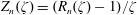 $Z_{n}(\unicode[STIX]{x1D701})=(R_{n}(\unicode[STIX]{x1D701})-1)/\unicode[STIX]{x1D701}$
.
$Z_{n}(\unicode[STIX]{x1D701})=(R_{n}(\unicode[STIX]{x1D701})-1)/\unicode[STIX]{x1D701}$
.
Moreover, we can do even better than (3.100). We shall not be satisfied just by approximating the asymptotic trend
 ${\sim}1/\unicode[STIX]{x1D701}$
for
${\sim}1/\unicode[STIX]{x1D701}$
for
 $\unicode[STIX]{x1D701}\gg 1$
, and hope for the best. For large
$\unicode[STIX]{x1D701}\gg 1$
, and hope for the best. For large
 $\unicode[STIX]{x1D701}$
, the correct asymptotic expansions are
$\unicode[STIX]{x1D701}$
, the correct asymptotic expansions are
 $Z(\unicode[STIX]{x1D701})\rightarrow -1/\unicode[STIX]{x1D701}$
and
$Z(\unicode[STIX]{x1D701})\rightarrow -1/\unicode[STIX]{x1D701}$
and
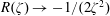 $R(\unicode[STIX]{x1D701})\rightarrow -1/(2\unicode[STIX]{x1D701}^{2})$
. By prescribing
$R(\unicode[STIX]{x1D701})\rightarrow -1/(2\unicode[STIX]{x1D701}^{2})$
. By prescribing
 $a_{n-1}/b_{n}=-1$
for
$a_{n-1}/b_{n}=-1$
for
 $Z(\unicode[STIX]{x1D701})$
, and
$Z(\unicode[STIX]{x1D701})$
, and
 $a_{n-2}/b_{n}=-1/2$
for
$a_{n-2}/b_{n}=-1/2$
for
 $R(\unicode[STIX]{x1D701})$
, we will obtain correct asymptotic behaviour of these functions, at least at the first order. By doing this, we are not ‘destroying’ the Padé approximation, since it is easy to argue that if an
$R(\unicode[STIX]{x1D701})$
, we will obtain correct asymptotic behaviour of these functions, at least at the first order. By doing this, we are not ‘destroying’ the Padé approximation, since it is easy to argue that if an
 $n$
-pole approximation is determined to be sufficient for small
$n$
-pole approximation is determined to be sufficient for small
 $\unicode[STIX]{x1D701}$
values, we can just add one more pole and use that one to control the asymptotic behaviour for large
$\unicode[STIX]{x1D701}$
values, we can just add one more pole and use that one to control the asymptotic behaviour for large
 $\unicode[STIX]{x1D701}$
values. Of course, we will always use at least the first term in the expansion for
$\unicode[STIX]{x1D701}$
values. Of course, we will always use at least the first term in the expansion for
 $\unicode[STIX]{x1D701}\ll 1$
, that yields
$\unicode[STIX]{x1D701}\ll 1$
, that yields
 $a_{0}=i\sqrt{\unicode[STIX]{x03C0}}$
for
$a_{0}=i\sqrt{\unicode[STIX]{x03C0}}$
for
 $Z_{n}(\unicode[STIX]{x1D701})$
and
$Z_{n}(\unicode[STIX]{x1D701})$
and
 $a_{0}=1$
for
$a_{0}=1$
for
 $R_{n}(\unicode[STIX]{x1D701})$
, otherwise the functions will have incorrect values at
$R_{n}(\unicode[STIX]{x1D701})$
, otherwise the functions will have incorrect values at
 $\unicode[STIX]{x1D701}=0$
. The ‘smart’ choices worth considering therefore can be summarized as
$\unicode[STIX]{x1D701}=0$
. The ‘smart’ choices worth considering therefore can be summarized as
 $$\begin{eqnarray}\displaystyle \displaystyle Z_{n}(\unicode[STIX]{x1D701}) & = & \displaystyle \frac{i\sqrt{\unicode[STIX]{x03C0}}+a_{1}\unicode[STIX]{x1D701}+\cdots +a_{n-1}\unicode[STIX]{x1D701}^{n-1}}{1+b_{1}\unicode[STIX]{x1D701}+\cdots +b_{n-1}\unicode[STIX]{x1D701}^{n-1}-a_{n-1}\unicode[STIX]{x1D701}^{n}};\nonumber\\ \displaystyle \displaystyle R_{n}(\unicode[STIX]{x1D701}) & = & \displaystyle \frac{1+a_{1}\unicode[STIX]{x1D701}+\cdots +a_{n-2}\unicode[STIX]{x1D701}^{n-2}}{1+b_{1}\unicode[STIX]{x1D701}+\cdots +b_{n-1}\unicode[STIX]{x1D701}^{n-1}-2a_{n-2}\unicode[STIX]{x1D701}^{n}},\end{eqnarray}$$
and have a property to correctly match the
 $Z$
and
$Z$
and
 $R$
functions at
$R$
functions at
 $\unicode[STIX]{x1D701}=0$
and, have the correct first-order asymptotic expansion at
$\unicode[STIX]{x1D701}=0$
and, have the correct first-order asymptotic expansion at
 $\unicode[STIX]{x1D701}\gg 1$
. The one-pole approximant
$\unicode[STIX]{x1D701}\gg 1$
. The one-pole approximant
 $R_{1}(\unicode[STIX]{x1D701})$
is an exception, and can be defined only as
$R_{1}(\unicode[STIX]{x1D701})$
is an exception, and can be defined only as
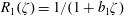 $R_{1}(\unicode[STIX]{x1D701})=1/(1+b_{1}\unicode[STIX]{x1D701})$
. This function obviously cannot have correct asymptotic expansion
$R_{1}(\unicode[STIX]{x1D701})=1/(1+b_{1}\unicode[STIX]{x1D701})$
. This function obviously cannot have correct asymptotic expansion
 ${\sim}1/\unicode[STIX]{x1D701}^{2}$
and the only possibility is to use
${\sim}1/\unicode[STIX]{x1D701}^{2}$
and the only possibility is to use
 $\unicode[STIX]{x1D701}\ll 1$
expansion
$\unicode[STIX]{x1D701}\ll 1$
expansion
 $R_{1}(\unicode[STIX]{x1D701})=1/(1+b_{1}\unicode[STIX]{x1D701})=1+i\sqrt{\unicode[STIX]{x03C0}}\unicode[STIX]{x1D701}$
, which yields
$R_{1}(\unicode[STIX]{x1D701})=1/(1+b_{1}\unicode[STIX]{x1D701})=1+i\sqrt{\unicode[STIX]{x03C0}}\unicode[STIX]{x1D701}$
, which yields
 $b_{1}=-i\sqrt{\unicode[STIX]{x03C0}}$
and
$b_{1}=-i\sqrt{\unicode[STIX]{x03C0}}$
and
 $$\begin{eqnarray}R_{1}(\unicode[STIX]{x1D701})=\frac{1}{1-i\sqrt{\unicode[STIX]{x03C0}}\unicode[STIX]{x1D701}}.\end{eqnarray}$$
The one-pole approximant
 $Z_{1}(\unicode[STIX]{x1D701})$
can be obtained directly from the definition (3.101), that yields
$Z_{1}(\unicode[STIX]{x1D701})$
can be obtained directly from the definition (3.101), that yields
 $$\begin{eqnarray}Z_{1}(\unicode[STIX]{x1D701})=\frac{i\sqrt{\unicode[STIX]{x03C0}}}{1-i\sqrt{\unicode[STIX]{x03C0}}\unicode[STIX]{x1D701}},\end{eqnarray}$$
and that has correct asymptotic behaviour
 $Z_{1}(\unicode[STIX]{x1D701})\rightarrow -1/\unicode[STIX]{x1D701}$
for large
$Z_{1}(\unicode[STIX]{x1D701})\rightarrow -1/\unicode[STIX]{x1D701}$
for large
 $\unicode[STIX]{x1D701}$
values, even though it has only precision
$\unicode[STIX]{x1D701}$
values, even though it has only precision
 $o(\unicode[STIX]{x1D701}^{0})$
for small
$o(\unicode[STIX]{x1D701}^{0})$
for small
 $\unicode[STIX]{x1D701}$
values. Perhaps curiously, in this case
$\unicode[STIX]{x1D701}$
values. Perhaps curiously, in this case
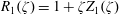 $R_{1}(\unicode[STIX]{x1D701})=1+\unicode[STIX]{x1D701}Z_{1}(\unicode[STIX]{x1D701})$
exactly. Alternatively, if the precision for small
$R_{1}(\unicode[STIX]{x1D701})=1+\unicode[STIX]{x1D701}Z_{1}(\unicode[STIX]{x1D701})$
exactly. Alternatively, if the precision for small
 $\unicode[STIX]{x1D701}$
is more important than the exact asymptotic expansion for large
$\unicode[STIX]{x1D701}$
is more important than the exact asymptotic expansion for large
 $\unicode[STIX]{x1D701}$
, it is possible to increase the
$\unicode[STIX]{x1D701}$
, it is possible to increase the
 $Z_{1}$
precision to
$Z_{1}$
precision to
 $o(\unicode[STIX]{x1D701}^{1})$
and write
$o(\unicode[STIX]{x1D701}^{1})$
and write
 $Z_{1}(\unicode[STIX]{x1D701})=i\sqrt{\unicode[STIX]{x03C0}}/(1-2i\unicode[STIX]{x1D701}/\sqrt{\unicode[STIX]{x03C0}})$
. In this case
$Z_{1}(\unicode[STIX]{x1D701})=i\sqrt{\unicode[STIX]{x03C0}}/(1-2i\unicode[STIX]{x1D701}/\sqrt{\unicode[STIX]{x03C0}})$
. In this case
 $R_{1}(\unicode[STIX]{x1D701})\neq 1+\unicode[STIX]{x1D701}Z_{1}(\unicode[STIX]{x1D701})$
exactly, and the functions are equal only for small
$R_{1}(\unicode[STIX]{x1D701})\neq 1+\unicode[STIX]{x1D701}Z_{1}(\unicode[STIX]{x1D701})$
exactly, and the functions are equal only for small
 $\unicode[STIX]{x1D701}$
and only with precision
$\unicode[STIX]{x1D701}$
and only with precision
 $o(\unicode[STIX]{x1D701}^{1})$
.
$o(\unicode[STIX]{x1D701}^{1})$
.
Right now, in the definition (3.101), we just used 1 pole for the asymptotic series of
 $Z(\unicode[STIX]{x1D701})$
and
$Z(\unicode[STIX]{x1D701})$
and
 $R(\unicode[STIX]{x1D701})$
, but one can naturally use more poles. By opening the possibility of increasing the number of matching asymptotic points in the
$R(\unicode[STIX]{x1D701})$
, but one can naturally use more poles. By opening the possibility of increasing the number of matching asymptotic points in the
 $n$
-pole Padé approximation (3.101), the number of possible approximants for a given
$n$
-pole Padé approximation (3.101), the number of possible approximants for a given
 $n$
naturally increases. To keep track of all the possibilities, we obviously need some kind of classification scheme. It is useful to modify the usual 1-index Padé series notation for
$n$
naturally increases. To keep track of all the possibilities, we obviously need some kind of classification scheme. It is useful to modify the usual 1-index Padé series notation for
 $Z_{n}(\unicode[STIX]{x1D701})$
and
$Z_{n}(\unicode[STIX]{x1D701})$
and
 $R_{n}(\unicode[STIX]{x1D701})$
functions (that only specify the number of poles), to a two index notation
$R_{n}(\unicode[STIX]{x1D701})$
functions (that only specify the number of poles), to a two index notation
 $Z_{n,n^{\prime }}(\unicode[STIX]{x1D701})$
,
$Z_{n,n^{\prime }}(\unicode[STIX]{x1D701})$
,
 $R_{n,n^{\prime }}(\unicode[STIX]{x1D701})$
. Now we have a wide range of possibilities how to define
$R_{n,n^{\prime }}(\unicode[STIX]{x1D701})$
. Now we have a wide range of possibilities how to define
 $n,n^{\prime }$
and there is no clear ‘natural’ winner.
$n,n^{\prime }$
and there is no clear ‘natural’ winner.
There are two different existing notations (likely more), introduced by Martín et al. (Reference Martín, Donoso and Zamudio-Cristi1980) and by Hedrick & Leboeuf (Reference Hedrick and Leboeuf1992), that consider
 $Z_{n,n^{\prime }}(\unicode[STIX]{x1D701})$
Padé approximants. The first reference defines
$Z_{n,n^{\prime }}(\unicode[STIX]{x1D701})$
Padé approximants. The first reference defines
 $n=\text{number}$
of points (equations) used in the power-series expansion, and
$n=\text{number}$
of points (equations) used in the power-series expansion, and
 $n^{\prime }=\text{number}$
of points (equations) used in the asymptotic series expansion. Even though perhaps clear, for example three-pole approximants in this notation are expressed as
$n^{\prime }=\text{number}$
of points (equations) used in the asymptotic series expansion. Even though perhaps clear, for example three-pole approximants in this notation are expressed as
 $Z_{5,1},Z_{4,2},Z_{3,3}$
etc., to get the number of poles (which is the most important information), one has to calculate
$Z_{5,1},Z_{4,2},Z_{3,3}$
etc., to get the number of poles (which is the most important information), one has to calculate
 $(n+n^{\prime })/2$
. When using a lot of different approximants, this notation is a bit confusing and is rarely used.
$(n+n^{\prime })/2$
. When using a lot of different approximants, this notation is a bit confusing and is rarely used.
The notation of Hedrick & Leboeuf (Reference Hedrick and Leboeuf1992) can be interpreted as defining
 $Z_{n,n^{\prime }}$
with
$Z_{n,n^{\prime }}$
with
 $n=\text{ number}$
of poles (which we like), and
$n=\text{ number}$
of poles (which we like), and
 $n^{\prime }=\text{number}$
of additional poles in the asymptotic expansion that is used, compared to some ‘minimally interesting’ or ‘basic’ definition
$n^{\prime }=\text{number}$
of additional poles in the asymptotic expansion that is used, compared to some ‘minimally interesting’ or ‘basic’ definition
 $Z_{n}$
, that can be denoted as
$Z_{n}$
, that can be denoted as
 $Z_{n,0}$
(which we like too). The problem with the notation of Hedrick & Leboeuf (Reference Hedrick and Leboeuf1992) is with the definition of the ‘basic’
$Z_{n,0}$
(which we like too). The problem with the notation of Hedrick & Leboeuf (Reference Hedrick and Leboeuf1992) is with the definition of the ‘basic’
 $Z_{n,0}$
, since the number of asymptotic points used in the definition of
$Z_{n,0}$
, since the number of asymptotic points used in the definition of
 $Z_{n,0}$
keeps changing with
$Z_{n,0}$
keeps changing with
 $n$
(and is actually equal to
$n$
(and is actually equal to
 $n$
). The notation is physically motivated, but the motivation is difficult to follow. The
$n$
). The notation is physically motivated, but the motivation is difficult to follow. The
 $Z_{2,0}$
is defined with 2 asymptotic points,
$Z_{2,0}$
is defined with 2 asymptotic points,
 $Z_{3,0}$
with 3 asymptotic points and so on. This can be easily deduced from their definitions of
$Z_{3,0}$
with 3 asymptotic points and so on. This can be easily deduced from their definitions of
 $Z_{2}-Z_{5}$
, as we will discuss later. We find this notation confusing.
$Z_{2}-Z_{5}$
, as we will discuss later. We find this notation confusing.
Importantly, both mentioned notations consider the Padé approximants to
 $Z(\unicode[STIX]{x1D701})$
. We do not really care about
$Z(\unicode[STIX]{x1D701})$
. We do not really care about
 $Z(\unicode[STIX]{x1D701})$
, since all the kinetic moments are formulated with
$Z(\unicode[STIX]{x1D701})$
, since all the kinetic moments are formulated with
 $R(\unicode[STIX]{x1D701})$
at this stage. We want to calculate direct Padé approximants to
$R(\unicode[STIX]{x1D701})$
at this stage. We want to calculate direct Padé approximants to
 $R(\unicode[STIX]{x1D701})$
, which is actually slightly less analytically complicated for a given
$R(\unicode[STIX]{x1D701})$
, which is actually slightly less analytically complicated for a given
 $n$
. Here we define the 2-index Padé approximation to the plasma response function
$n$
. Here we define the 2-index Padé approximation to the plasma response function
 $R(\unicode[STIX]{x1D701})$
simply as
$R(\unicode[STIX]{x1D701})$
simply as
i.e. as having asymptote
 $-1/(2\unicode[STIX]{x1D701}^{2})$
for large
$-1/(2\unicode[STIX]{x1D701}^{2})$
for large
 $\unicode[STIX]{x1D701}$
, and notation
$\unicode[STIX]{x1D701}$
, and notation
 $R_{n,n^{\prime }}(\unicode[STIX]{x1D701})$
means that
$R_{n,n^{\prime }}(\unicode[STIX]{x1D701})$
means that
 $n^{\prime }$
additional asymptotic points are used compared to the basic definition
$n^{\prime }$
additional asymptotic points are used compared to the basic definition
 $R_{n,0}(\unicode[STIX]{x1D701})$
. The notation feels natural, and the
$R_{n,0}(\unicode[STIX]{x1D701})$
. The notation feels natural, and the
 $n^{\prime }=0$
index helps us to orient in the hierarchy of many possible
$n^{\prime }=0$
index helps us to orient in the hierarchy of many possible
 $R(\unicode[STIX]{x1D701})$
approximants. It is easy to remember that this asymptotic profile is the minimum ‘desired’ profile that correctly captures the zeroth-order (density) moment, and any profile with less asymptotic points should be avoided if possible. The
$R(\unicode[STIX]{x1D701})$
approximants. It is easy to remember that this asymptotic profile is the minimum ‘desired’ profile that correctly captures the zeroth-order (density) moment, and any profile with less asymptotic points should be avoided if possible. The
 $R_{n,0}(\unicode[STIX]{x1D701})$
has power-series precision
$R_{n,0}(\unicode[STIX]{x1D701})$
has power-series precision
 $o(\unicode[STIX]{x1D701}^{2n-3})$
and asymptotic-series precision
$o(\unicode[STIX]{x1D701}^{2n-3})$
and asymptotic-series precision
 $o(\unicode[STIX]{x1D701}^{-2})$
, so
$o(\unicode[STIX]{x1D701}^{-2})$
, so
 $R_{n,n^{\prime }}(\unicode[STIX]{x1D701})$
has precision
$R_{n,n^{\prime }}(\unicode[STIX]{x1D701})$
has precision
 $o(\unicode[STIX]{x1D701}^{2n-3-n^{\prime }})$
and
$o(\unicode[STIX]{x1D701}^{2n-3-n^{\prime }})$
and
 $o(\unicode[STIX]{x1D701}^{-2-n^{\prime }})$
.
$o(\unicode[STIX]{x1D701}^{-2-n^{\prime }})$
.
Of course, we want to make the
 $R_{n,n^{\prime }}(\unicode[STIX]{x1D701})$
and
$R_{n,n^{\prime }}(\unicode[STIX]{x1D701})$
and
 $Z_{n,n^{\prime }}(\unicode[STIX]{x1D701})$
definitions fully consistent, and
$Z_{n,n^{\prime }}(\unicode[STIX]{x1D701})$
definitions fully consistent, and
 $Z_{n,n^{\prime }}(\unicode[STIX]{x1D701})$
is defined so that
$Z_{n,n^{\prime }}(\unicode[STIX]{x1D701})$
is defined so that
 $$\begin{eqnarray}R_{n,n^{\prime }}(\unicode[STIX]{x1D701})=1+\unicode[STIX]{x1D701}Z_{n,n^{\prime }}(\unicode[STIX]{x1D701}),\end{eqnarray}$$
is satisfied. This dictates that in comparison to
 $Z_{n}(\unicode[STIX]{x1D701})$
definition (3.101), two additional asymptotic points must be used to define the
$Z_{n}(\unicode[STIX]{x1D701})$
definition (3.101), two additional asymptotic points must be used to define the
 $Z_{n,0}(\unicode[STIX]{x1D701})$
. We have no other choice and when calculating the
$Z_{n,0}(\unicode[STIX]{x1D701})$
. We have no other choice and when calculating the
 $Z_{n,n^{\prime }}(\unicode[STIX]{x1D701})$
, we have to start counting from
$Z_{n,n^{\prime }}(\unicode[STIX]{x1D701})$
, we have to start counting from
 $n^{\prime }=-2$
, and we define
$n^{\prime }=-2$
, and we define
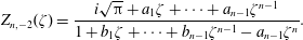 $$\begin{eqnarray}Z_{n,-2}(\unicode[STIX]{x1D701})=\frac{i\sqrt{\unicode[STIX]{x03C0}}+a_{1}\unicode[STIX]{x1D701}+\cdots +a_{n-1}\unicode[STIX]{x1D701}^{n-1}}{1+b_{1}\unicode[STIX]{x1D701}+\cdots +b_{n-1}\unicode[STIX]{x1D701}^{n-1}-a_{n-1}\unicode[STIX]{x1D701}^{n}}.\end{eqnarray}$$
When calculating the hierarchy of plasma dispersion functions
 $Z(\unicode[STIX]{x1D701})$
, the
$Z(\unicode[STIX]{x1D701})$
, the
 $-2$
index is actually a nice reminder that we are two asymptotic points short of the ‘desired’ profile (3.104) for the plasma response function
$-2$
index is actually a nice reminder that we are two asymptotic points short of the ‘desired’ profile (3.104) for the plasma response function
 $R(\unicode[STIX]{x1D701})$
. We want to feel fully confident that we understand both Padé approximants
$R(\unicode[STIX]{x1D701})$
. We want to feel fully confident that we understand both Padé approximants
 $R(\unicode[STIX]{x1D701})$
and
$R(\unicode[STIX]{x1D701})$
and
 $Z(\unicode[STIX]{x1D701})$
, and we will calculate two-pole and three-pole approximants for both functions. For four-pole approximants and above, we will only work with
$Z(\unicode[STIX]{x1D701})$
, and we will calculate two-pole and three-pole approximants for both functions. For four-pole approximants and above, we will only work with
 $R(\unicode[STIX]{x1D701})$
.
$R(\unicode[STIX]{x1D701})$
.
Padé approximants were also used for other interesting physical problems, such as developing analytic models for the Rayleigh–Taylor and Richtmyer–Meshkov instabilities (Zhou Reference Zhou2017a ,Reference Zhou b ).
3.3.1 Two-pole approximants of
$R(\unicode[STIX]{x1D701})$
and
$Z(\unicode[STIX]{x1D701})$


Let us be patient and go slowly. A general two-pole Padé approximant to
 $R(\unicode[STIX]{x1D701})$
is
$R(\unicode[STIX]{x1D701})$
is
 $$\begin{eqnarray}R_{2}(\unicode[STIX]{x1D701})=\frac{a_{0}}{1+b_{1}\unicode[STIX]{x1D701}+b_{2}\unicode[STIX]{x1D701}^{2}},\end{eqnarray}$$
where
 $a_{0}=1$
. The asymptotic expansion for large
$a_{0}=1$
. The asymptotic expansion for large
 $\unicode[STIX]{x1D701}$
values calculates as
$\unicode[STIX]{x1D701}$
values calculates as
 $$\begin{eqnarray}\displaystyle \frac{a_{0}}{1+b_{1}\unicode[STIX]{x1D701}+b_{2}\unicode[STIX]{x1D701}^{2}} & = & \displaystyle \frac{a_{0}}{b_{2}\unicode[STIX]{x1D701}^{2}\left({\displaystyle \frac{1}{b_{2}\unicode[STIX]{x1D701}^{2}}}+{\displaystyle \frac{b_{1}}{b_{2}\unicode[STIX]{x1D701}}}+1\right)}\nonumber\\ \displaystyle & = & \displaystyle \frac{a_{0}}{b_{2}\unicode[STIX]{x1D701}^{2}}\left[1-\left(\frac{b_{1}}{b_{2}\unicode[STIX]{x1D701}}+\frac{1}{b_{2}\unicode[STIX]{x1D701}^{2}}\right)+\left(\frac{b_{1}}{b_{2}\unicode[STIX]{x1D701}}+\frac{1}{b_{2}\unicode[STIX]{x1D701}^{2}}\right)^{2}+\cdots \,\right]\nonumber\\ \displaystyle & = & \displaystyle \frac{a_{0}}{b_{2}\unicode[STIX]{x1D701}^{2}}-a_{0}\frac{b_{1}}{b_{2}^{2}\unicode[STIX]{x1D701}^{3}}+a_{0}\frac{b_{1}^{2}-b_{2}}{b_{2}^{3}\unicode[STIX]{x1D701}^{4}}+\cdots \,;\quad \unicode[STIX]{x1D701}\gg 1,\end{eqnarray}$$
and must be matched with the asymptotic expansion (3.67)
 $$\begin{eqnarray}R(\unicode[STIX]{x1D701})=-\frac{1}{2\unicode[STIX]{x1D701}^{2}}-\frac{0}{\unicode[STIX]{x1D701}^{3}}-\frac{3}{4\unicode[STIX]{x1D701}^{4}}+\cdots \,;\quad \unicode[STIX]{x1D701}\gg 1.\end{eqnarray}$$
Matching the first point implies
 $b_{2}=-2a_{0}$
, and this is how
$b_{2}=-2a_{0}$
, and this is how
 $R_{2,0}(\unicode[STIX]{x1D701})$
is defined. Then, matching with 2 equations for the small
$R_{2,0}(\unicode[STIX]{x1D701})$
is defined. Then, matching with 2 equations for the small
 $\unicode[STIX]{x1D701}$
expansion, equation (3.36), the classical Padé approach yields
$\unicode[STIX]{x1D701}$
expansion, equation (3.36), the classical Padé approach yields
 $$\begin{eqnarray}R_{2,0}(\unicode[STIX]{x1D701})=\frac{a_{0}}{1+b_{1}\unicode[STIX]{x1D701}-2a_{0}\unicode[STIX]{x1D701}^{2}}=\underbrace{1}_{=c_{0}}+\underbrace{i\sqrt{\unicode[STIX]{x03C0}}}_{=c_{1}}\unicode[STIX]{x1D701};\quad \Rightarrow \quad R_{2,0}(\unicode[STIX]{x1D701})=\frac{1}{1-i\sqrt{\unicode[STIX]{x03C0}}\unicode[STIX]{x1D701}-2\unicode[STIX]{x1D701}^{2}}.\end{eqnarray}$$
To match additional asymptotic point (and to potentially find
 $R_{2,1}(\unicode[STIX]{x1D701})$
), dictates that
$R_{2,1}(\unicode[STIX]{x1D701})$
), dictates that
 $b_{1}=0$
. However, the resulting function
$b_{1}=0$
. However, the resulting function
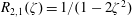 $R_{2,1}(\unicode[STIX]{x1D701})=1/(1-2\unicode[STIX]{x1D701}^{2})$
does not have any imaginary part for real valued
$R_{2,1}(\unicode[STIX]{x1D701})=1/(1-2\unicode[STIX]{x1D701}^{2})$
does not have any imaginary part for real valued
 $\unicode[STIX]{x1D701}$
, since it uses too many asymptotic points and the Landau residue is not accounted for. Therefore, the
$\unicode[STIX]{x1D701}$
, since it uses too many asymptotic points and the Landau residue is not accounted for. Therefore, the
 $R_{2,1}(\unicode[STIX]{x1D701})$
does not represent a valuable approximation of
$R_{2,1}(\unicode[STIX]{x1D701})$
does not represent a valuable approximation of
 $R(\unicode[STIX]{x1D701})$
, and this approximant is eliminated.
$R(\unicode[STIX]{x1D701})$
, and this approximant is eliminated.
Let us now explore possible two-pole approximations of
 $Z(\unicode[STIX]{x1D701})$
. A general two-pole approximant is defined as
$Z(\unicode[STIX]{x1D701})$
. A general two-pole approximant is defined as
 $$\begin{eqnarray}\displaystyle Z_{2}(\unicode[STIX]{x1D701})=\frac{a_{0}+a_{1}\unicode[STIX]{x1D701}}{1+b_{1}\unicode[STIX]{x1D701}+b_{2}\unicode[STIX]{x1D701}^{2}}, & & \displaystyle\end{eqnarray}$$
and has the following asymptotic expansion for large
 $\unicode[STIX]{x1D701}$
values
$\unicode[STIX]{x1D701}$
values
 $$\begin{eqnarray}\displaystyle \frac{a_{0}+a_{1}\unicode[STIX]{x1D701}}{1+b_{1}\unicode[STIX]{x1D701}+b_{2}\unicode[STIX]{x1D701}^{2}} & = & \displaystyle \left(\frac{a_{1}}{b_{2}}\right)\frac{1}{\unicode[STIX]{x1D701}}+\left(\frac{a_{0}}{b_{2}}-\frac{a_{1}b_{1}}{b_{2}^{2}}\right)\frac{1}{\unicode[STIX]{x1D701}^{2}}\nonumber\\ \displaystyle & & \displaystyle +\,\left(-\frac{a_{0}b_{1}}{b_{2}^{2}}+\frac{a_{1}(b_{1}^{2}-b_{2})}{b_{2}^{3}}\right)\frac{1}{\unicode[STIX]{x1D701}^{3}}+\cdots \,;\quad \unicode[STIX]{x1D701}\gg 1.\end{eqnarray}$$
The
 $Z(\unicode[STIX]{x1D701})$
has asymptotic expansion
$Z(\unicode[STIX]{x1D701})$
has asymptotic expansion
 $$\begin{eqnarray}Z(\unicode[STIX]{x1D701})=-\frac{1}{\unicode[STIX]{x1D701}}-\frac{0}{\unicode[STIX]{x1D701}^{2}}-\frac{1}{2\unicode[STIX]{x1D701}^{3}}+\cdots \,;\quad \unicode[STIX]{x1D701}\gg 1,\end{eqnarray}$$
so by matching with
 $1/\unicode[STIX]{x1D701}$
implies
$1/\unicode[STIX]{x1D701}$
implies
 $b_{2}=-a_{1}$
(as already used previously) that defines
$b_{2}=-a_{1}$
(as already used previously) that defines
 $Z_{2,-2}$
(remember, we are starting to count with
$Z_{2,-2}$
(remember, we are starting to count with
 $n^{\prime }=-2$
). By further matching with
$n^{\prime }=-2$
). By further matching with
 $1/\unicode[STIX]{x1D701}^{2}$
implies
$1/\unicode[STIX]{x1D701}^{2}$
implies
 $b_{1}=-a_{0}$
, that defines
$b_{1}=-a_{0}$
, that defines
 $Z_{2,-1}$
, and by further matching with
$Z_{2,-1}$
, and by further matching with
 $1/\unicode[STIX]{x1D701}^{3}$
implies
$1/\unicode[STIX]{x1D701}^{3}$
implies
 $a_{1}=2$
, that defines
$a_{1}=2$
, that defines
 $Z_{2,0}$
.
$Z_{2,0}$
.
The calculation is continued by matching with the power series for small
 $\unicode[STIX]{x1D701}$
values, i.e. by using the classical Padé approach, that is described as
$\unicode[STIX]{x1D701}$
values, i.e. by using the classical Padé approach, that is described as
 $$\begin{eqnarray}\displaystyle Z_{2,-2}(\unicode[STIX]{x1D701})=\frac{a_{0}+a_{1}\unicode[STIX]{x1D701}}{1+b_{1}\unicode[STIX]{x1D701}-a_{1}\unicode[STIX]{x1D701}^{2}}=\underbrace{i\sqrt{\unicode[STIX]{x03C0}}}_{=c_{0}}\underbrace{-2}_{=c_{1}}\unicode[STIX]{x1D701}\underbrace{-i\sqrt{\unicode[STIX]{x03C0}}}_{=c_{2}}\unicode[STIX]{x1D701}^{2}, & & \displaystyle\end{eqnarray}$$
and the solution is
 $$\begin{eqnarray}\displaystyle Z_{2,-2}(\unicode[STIX]{x1D701})=\frac{i\sqrt{\unicode[STIX]{x03C0}}+{\displaystyle \frac{4-\unicode[STIX]{x03C0}}{\unicode[STIX]{x03C0}-2}}\unicode[STIX]{x1D701}}{1-{\displaystyle \frac{i\sqrt{\unicode[STIX]{x03C0}}}{\unicode[STIX]{x03C0}-2}}\unicode[STIX]{x1D701}-{\displaystyle \frac{4-\unicode[STIX]{x03C0}}{\unicode[STIX]{x03C0}-2}}\unicode[STIX]{x1D701}^{2}}. & & \displaystyle\end{eqnarray}$$
Continuing with
 $Z_{2,-1}(\unicode[STIX]{x1D701})$
, i.e. by using one more additional asymptotic term that dictates
$Z_{2,-1}(\unicode[STIX]{x1D701})$
, i.e. by using one more additional asymptotic term that dictates
 $b_{1}=-a_{0}$
, the matching with the power series yields
$b_{1}=-a_{0}$
, the matching with the power series yields
 $$\begin{eqnarray}Z_{2,-1}(\unicode[STIX]{x1D701})=\frac{a_{0}+a_{1}\unicode[STIX]{x1D701}}{1-a_{0}\unicode[STIX]{x1D701}-a_{1}\unicode[STIX]{x1D701}^{2}}=i\sqrt{\unicode[STIX]{x03C0}}-2\unicode[STIX]{x1D701};\quad \Rightarrow \quad Z_{2,-1}(\unicode[STIX]{x1D701})=\frac{i\sqrt{\unicode[STIX]{x03C0}}+(\unicode[STIX]{x03C0}-2)\unicode[STIX]{x1D701}}{1-i\sqrt{\unicode[STIX]{x03C0}}\unicode[STIX]{x1D701}-(\unicode[STIX]{x03C0}-2)\unicode[STIX]{x1D701}^{2}}.\end{eqnarray}$$
Similarly, considering
 $Z_{2,0}(\unicode[STIX]{x1D701})$
yields
$Z_{2,0}(\unicode[STIX]{x1D701})$
yields
 $$\begin{eqnarray}Z_{2,0}(\unicode[STIX]{x1D701})=\frac{a_{0}+2\unicode[STIX]{x1D701}}{1-a_{0}\unicode[STIX]{x1D701}-2\unicode[STIX]{x1D701}^{2}}=i\sqrt{\unicode[STIX]{x03C0}};\quad \Rightarrow \quad Z_{2,0}(\unicode[STIX]{x1D701})=\frac{i\sqrt{\unicode[STIX]{x03C0}}+2\unicode[STIX]{x1D701}}{1-i\sqrt{\unicode[STIX]{x03C0}}\unicode[STIX]{x1D701}-2\unicode[STIX]{x1D701}^{2}}.\end{eqnarray}$$
Obviously,
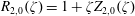 $R_{2,0}(\unicode[STIX]{x1D701})=1+\unicode[STIX]{x1D701}Z_{2,0}(\unicode[STIX]{x1D701})$
exactly.
$R_{2,0}(\unicode[STIX]{x1D701})=1+\unicode[STIX]{x1D701}Z_{2,0}(\unicode[STIX]{x1D701})$
exactly.
3.3.2 Three-pole approximants of
$R(\unicode[STIX]{x1D701})$
and
$Z(\unicode[STIX]{x1D701})$


A general three-pole approximant of
 $R(\unicode[STIX]{x1D701})$
is
$R(\unicode[STIX]{x1D701})$
is
 $$\begin{eqnarray}\displaystyle R_{3}(\unicode[STIX]{x1D701})=\frac{a_{0}+a_{1}\unicode[STIX]{x1D701}}{1+b_{1}\unicode[STIX]{x1D701}+b_{2}\unicode[STIX]{x1D701}^{2}+b_{3}\unicode[STIX]{x1D701}^{3}}. & & \displaystyle\end{eqnarray}$$
The asymptotic expansion calculates as
 $$\begin{eqnarray}\displaystyle \frac{1}{1+b_{1}\unicode[STIX]{x1D701}+b_{2}\unicode[STIX]{x1D701}^{2}+b_{3}\unicode[STIX]{x1D701}^{3}} & = & \displaystyle \frac{1}{b_{3}\unicode[STIX]{x1D701}^{3}\left({\displaystyle \frac{1}{b_{3}\unicode[STIX]{x1D701}^{3}}}+{\displaystyle \frac{b_{1}}{b_{3}\unicode[STIX]{x1D701}^{2}}}+{\displaystyle \frac{b_{2}}{b_{3}\unicode[STIX]{x1D701}}}+1\right)}\nonumber\\ \displaystyle & = & \displaystyle \frac{1}{b_{3}\unicode[STIX]{x1D701}^{3}}\left[1-\left(\frac{b_{2}}{b_{3}\unicode[STIX]{x1D701}}+\frac{b_{1}}{b_{3}\unicode[STIX]{x1D701}^{2}}+\frac{1}{b_{3}\unicode[STIX]{x1D701}^{3}}\right)\vphantom{\left(\frac{1}{b_{3}\unicode[STIX]{x1D701}^{3}}\right)^{2}}\right.\nonumber\\ \displaystyle & & \displaystyle \left.+\,\left(\frac{b_{2}}{b_{3}\unicode[STIX]{x1D701}}+\frac{b_{1}}{b_{3}\unicode[STIX]{x1D701}^{2}}+\frac{1}{b_{3}\unicode[STIX]{x1D701}^{3}}\right)^{2}+\cdots \,\right]\nonumber\\ \displaystyle & = & \displaystyle \frac{1}{b_{3}\unicode[STIX]{x1D701}^{3}}\left[1-\frac{1}{\unicode[STIX]{x1D701}}\frac{b_{2}}{b_{3}}+\frac{1}{\unicode[STIX]{x1D701}^{2}}\left(-\frac{b_{1}}{b_{3}}+\frac{b_{2}^{2}}{b_{3}^{2}}\right)+\cdots \,\right]\nonumber\\ \displaystyle & = & \displaystyle \frac{1}{b_{3}\unicode[STIX]{x1D701}^{3}}-\frac{b_{2}}{b_{3}^{2}\unicode[STIX]{x1D701}^{4}}+\frac{b_{2}^{2}-b_{1}b_{3}}{b_{3}^{3}\unicode[STIX]{x1D701}^{5}}+\cdots \,,\end{eqnarray}$$
so that
 $$\begin{eqnarray}\displaystyle \frac{a_{0}+a_{1}\unicode[STIX]{x1D701}}{1+b_{1}\unicode[STIX]{x1D701}+b_{2}\unicode[STIX]{x1D701}^{2}+b_{3}\unicode[STIX]{x1D701}^{3}} & = & \displaystyle \frac{a_{1}}{b_{3}\unicode[STIX]{x1D701}^{2}}+\frac{1}{\unicode[STIX]{x1D701}^{3}}\left(\frac{a_{0}}{b_{3}}-\frac{a_{1}b_{2}}{b_{3}^{2}}\right)\nonumber\\ \displaystyle & & \displaystyle +\,\frac{1}{\unicode[STIX]{x1D701}^{4}}\left(-\frac{a_{0}b_{2}}{b_{3}^{2}}+a_{1}\frac{b_{2}^{2}-b_{1}b_{3}}{b_{3}^{3}}\right)+\cdots\end{eqnarray}$$
For
 $R_{3,0}(\unicode[STIX]{x1D701})$
this implies
$R_{3,0}(\unicode[STIX]{x1D701})$
this implies
 $b_{3}=-2a_{1}$
, for
$b_{3}=-2a_{1}$
, for
 $R_{3,1}(\unicode[STIX]{x1D701})$
additionally
$R_{3,1}(\unicode[STIX]{x1D701})$
additionally
 $b_{2}=-2a_{0}$
and for
$b_{2}=-2a_{0}$
and for
 $R_{3,2}(\unicode[STIX]{x1D701})$
also
$R_{3,2}(\unicode[STIX]{x1D701})$
also
 $b_{1}=3a_{1}$
. The asymptotic expansions (3.120) can become very long for higher orders of
$b_{1}=3a_{1}$
. The asymptotic expansions (3.120) can become very long for higher orders of
 $\unicode[STIX]{x1D701}$
, especially when more poles are considered. It is beneficial to write down the following scheme, where in each line, we advance the matching with one more asymptotic point,
$\unicode[STIX]{x1D701}$
, especially when more poles are considered. It is beneficial to write down the following scheme, where in each line, we advance the matching with one more asymptotic point,
 $$\begin{eqnarray}\displaystyle \frac{a_{0}+a_{1}\unicode[STIX]{x1D701}}{1+b_{1}\unicode[STIX]{x1D701}+b_{2}\unicode[STIX]{x1D701}^{2}+b_{3}\unicode[STIX]{x1D701}^{3}}=\underbrace{\frac{a_{1}}{b_{3}}}_{=-1/2}\frac{1}{\unicode[STIX]{x1D701}^{2}}+\cdots \quad \Rightarrow \quad b_{3}=-2a_{1}; & & \displaystyle\end{eqnarray}$$
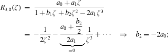 $$\begin{eqnarray}\displaystyle R_{3,0}(\unicode[STIX]{x1D701}) & = & \displaystyle \frac{a_{0}+a_{1}\unicode[STIX]{x1D701}}{1+b_{1}\unicode[STIX]{x1D701}+b_{2}\unicode[STIX]{x1D701}^{2}-2a_{1}\unicode[STIX]{x1D701}^{3}}\nonumber\\ \displaystyle & = & \displaystyle -\frac{1}{2\unicode[STIX]{x1D701}^{2}}-\underbrace{\frac{a_{0}+{\displaystyle \frac{b_{2}}{2}}}{2a_{1}}}_{=0}\frac{1}{\unicode[STIX]{x1D701}^{3}}+\cdots \quad \Rightarrow \quad b_{2}=-2a_{0};\end{eqnarray}$$
 $$\begin{eqnarray}\displaystyle R_{3,1}(\unicode[STIX]{x1D701}) & = & \displaystyle \frac{a_{0}+a_{1}\unicode[STIX]{x1D701}}{1+b_{1}\unicode[STIX]{x1D701}-2a_{0}\unicode[STIX]{x1D701}^{2}-2a_{1}\unicode[STIX]{x1D701}^{3}}\nonumber\\ \displaystyle & = & \displaystyle -\frac{1}{2\unicode[STIX]{x1D701}^{2}}-\underbrace{\frac{b_{1}}{4a_{1}}}_{=3/4}\frac{1}{\unicode[STIX]{x1D701}^{4}}+\cdots \quad \Rightarrow \quad b_{1}=3a_{1};\end{eqnarray}$$
 $$\begin{eqnarray}\displaystyle R_{3,2}(\unicode[STIX]{x1D701}) & = & \displaystyle \frac{a_{0}+a_{1}\unicode[STIX]{x1D701}}{1+3a_{1}\unicode[STIX]{x1D701}-2a_{0}\unicode[STIX]{x1D701}^{2}-2a_{1}\unicode[STIX]{x1D701}^{3}}\nonumber\\ \displaystyle & = & \displaystyle -\frac{1}{2\unicode[STIX]{x1D701}^{2}}-\frac{3}{4\unicode[STIX]{x1D701}^{4}}-\underbrace{\frac{1-3a_{0}}{4a_{1}}}_{=0}\frac{1}{\unicode[STIX]{x1D701}^{5}}+\cdots \quad \Rightarrow \quad a_{1}\rightarrow \infty .\end{eqnarray}$$
In the last expression the
 $a_{1}\rightarrow \infty$
since
$a_{1}\rightarrow \infty$
since
 $a_{0}=1$
, implying the
$a_{0}=1$
, implying the
 $R_{3,3}(\unicode[STIX]{x1D701})$
does not make sense and it is not defined. The scheme can be very quickly verified by using Maple (or Mathematica) software, by using command
$R_{3,3}(\unicode[STIX]{x1D701})$
does not make sense and it is not defined. The scheme can be very quickly verified by using Maple (or Mathematica) software, by using command
 $asympt(expression(\unicode[STIX]{x1D701}),\unicode[STIX]{x1D701},n)$
, where
$asympt(expression(\unicode[STIX]{x1D701}),\unicode[STIX]{x1D701},n)$
, where
 $\unicode[STIX]{x1D701}$
is the variable, and
$\unicode[STIX]{x1D701}$
is the variable, and
 $n$
prescribes the precision of the expansion that is calculated up to the
$n$
prescribes the precision of the expansion that is calculated up to the
 $o(\unicode[STIX]{x1D701}^{-n})$
order. Now by matching with the power series for small
$o(\unicode[STIX]{x1D701}^{-n})$
order. Now by matching with the power series for small
 $\unicode[STIX]{x1D701}$
values
$\unicode[STIX]{x1D701}$
values
 $$\begin{eqnarray}\displaystyle R_{3,0}(\unicode[STIX]{x1D701}) & = & \displaystyle \frac{a_{0}+a_{1}\unicode[STIX]{x1D701}}{1+b_{1}\unicode[STIX]{x1D701}+b_{2}\unicode[STIX]{x1D701}^{2}-2a_{1}\unicode[STIX]{x1D701}^{3}}=1+i\sqrt{\unicode[STIX]{x03C0}}\unicode[STIX]{x1D701}-2\unicode[STIX]{x1D701}^{2}-i\sqrt{\unicode[STIX]{x03C0}}\unicode[STIX]{x1D701}^{3};\end{eqnarray}$$
 $$\begin{eqnarray}\displaystyle R_{3,1}(\unicode[STIX]{x1D701}) & = & \displaystyle \frac{a_{0}+a_{1}\unicode[STIX]{x1D701}}{1+b_{1}\unicode[STIX]{x1D701}-2a_{0}\unicode[STIX]{x1D701}^{2}-2a_{1}\unicode[STIX]{x1D701}^{3}}=1+i\sqrt{\unicode[STIX]{x03C0}}\unicode[STIX]{x1D701}-2\unicode[STIX]{x1D701}^{2};\end{eqnarray}$$
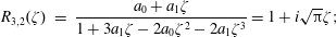 $$\begin{eqnarray}\displaystyle R_{3,2}(\unicode[STIX]{x1D701}) & = & \displaystyle \frac{a_{0}+a_{1}\unicode[STIX]{x1D701}}{1+3a_{1}\unicode[STIX]{x1D701}-2a_{0}\unicode[STIX]{x1D701}^{2}-2a_{1}\unicode[STIX]{x1D701}^{3}}=1+i\sqrt{\unicode[STIX]{x03C0}}\unicode[STIX]{x1D701};\end{eqnarray}$$
and the solutions are
 $$\begin{eqnarray}\displaystyle R_{3,0}(\unicode[STIX]{x1D701}) & = & \displaystyle \frac{1-i\sqrt{\unicode[STIX]{x03C0}}{\displaystyle \frac{\unicode[STIX]{x03C0}-3}{4-\unicode[STIX]{x03C0}}}\unicode[STIX]{x1D701}}{1-i{\displaystyle \frac{\sqrt{\unicode[STIX]{x03C0}}}{4-\unicode[STIX]{x03C0}}}\unicode[STIX]{x1D701}-{\displaystyle \frac{3\unicode[STIX]{x03C0}-8}{4-\unicode[STIX]{x03C0}}}\unicode[STIX]{x1D701}^{2}+2i\sqrt{\unicode[STIX]{x03C0}}{\displaystyle \frac{\unicode[STIX]{x03C0}-3}{4-\unicode[STIX]{x03C0}}}\unicode[STIX]{x1D701}^{3}};\end{eqnarray}$$
 $$\begin{eqnarray}\displaystyle R_{3,1}(\unicode[STIX]{x1D701}) & = & \displaystyle \frac{1-i{\displaystyle \frac{4-\unicode[STIX]{x03C0}}{\sqrt{\unicode[STIX]{x03C0}}}}\unicode[STIX]{x1D701}}{1-{\displaystyle \frac{4i}{\sqrt{\unicode[STIX]{x03C0}}}}\unicode[STIX]{x1D701}-2\unicode[STIX]{x1D701}^{2}+2i{\displaystyle \frac{4-\unicode[STIX]{x03C0}}{\sqrt{\unicode[STIX]{x03C0}}}}\unicode[STIX]{x1D701}^{3}};\end{eqnarray}$$
 $$\begin{eqnarray}\displaystyle R_{3,2}(\unicode[STIX]{x1D701}) & = & \displaystyle \frac{1-{\displaystyle \frac{i\sqrt{\unicode[STIX]{x03C0}}}{2}}\unicode[STIX]{x1D701}}{1-{\displaystyle \frac{3i\sqrt{\unicode[STIX]{x03C0}}}{2}}\unicode[STIX]{x1D701}-2\unicode[STIX]{x1D701}^{2}+i\sqrt{\unicode[STIX]{x03C0}}\unicode[STIX]{x1D701}^{3}}.\end{eqnarray}$$
A general three-pole approximant of
 $Z(\unicode[STIX]{x1D701})$
is
$Z(\unicode[STIX]{x1D701})$
is
 $$\begin{eqnarray}Z_{3}(\unicode[STIX]{x1D701})=\frac{a_{0}+a_{1}\unicode[STIX]{x1D701}+a_{2}\unicode[STIX]{x1D701}^{2}}{1+b_{1}\unicode[STIX]{x1D701}+b_{2}\unicode[STIX]{x1D701}^{2}+b_{3}\unicode[STIX]{x1D701}^{3}},\end{eqnarray}$$
and has the following asymptotic expansion
 $$\begin{eqnarray}\displaystyle \frac{a_{0}+a_{1}\unicode[STIX]{x1D701}+a_{2}\unicode[STIX]{x1D701}^{2}}{1+b_{1}\unicode[STIX]{x1D701}+b_{2}\unicode[STIX]{x1D701}^{2}+b_{3}\unicode[STIX]{x1D701}^{3}} & = & \displaystyle \frac{a_{2}}{b_{3}\unicode[STIX]{x1D701}}+\left(\frac{a_{1}}{b_{3}}-\frac{a_{2}b_{2}}{b_{3}^{2}}\right)\frac{1}{\unicode[STIX]{x1D701}^{2}}\nonumber\\ \displaystyle & & \displaystyle +\,\left(\frac{a_{0}}{b_{3}}-\frac{a_{1}b_{2}}{b_{3}^{2}}+\frac{a_{2}(b_{2}^{2}-b_{1}b_{3})}{b_{3}^{3}}\right)\frac{1}{\unicode[STIX]{x1D701}^{3}}+\cdots\end{eqnarray}$$
Matching the first asymptotic term implies
 $b_{3}=-a_{2}$
, which defines
$b_{3}=-a_{2}$
, which defines
 $Z_{3,-2}(\unicode[STIX]{x1D701})$
. For
$Z_{3,-2}(\unicode[STIX]{x1D701})$
. For
 $Z_{3,-1}(\unicode[STIX]{x1D701})$
the second term is matched as well and
$Z_{3,-1}(\unicode[STIX]{x1D701})$
the second term is matched as well and
 $b_{2}=-a_{1}$
. For
$b_{2}=-a_{1}$
. For
 $Z_{3,0}(\unicode[STIX]{x1D701})$
the third term is also matched and
$Z_{3,0}(\unicode[STIX]{x1D701})$
the third term is also matched and
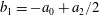 $b_{1}=-a_{0}+a_{2}/2$
. To go higher requires higher-order expansion (3.132). It is again easier to write down the asymptotic expansion scheme step by step
$b_{1}=-a_{0}+a_{2}/2$
. To go higher requires higher-order expansion (3.132). It is again easier to write down the asymptotic expansion scheme step by step
 $$\begin{eqnarray}\displaystyle & \displaystyle \frac{a_{0}+a_{1}\unicode[STIX]{x1D701}+a_{2}\unicode[STIX]{x1D701}^{2}}{1+b_{1}\unicode[STIX]{x1D701}+b_{2}\unicode[STIX]{x1D701}^{2}+b_{3}\unicode[STIX]{x1D701}^{3}}=\underbrace{\frac{a_{2}}{b_{3}}}_{=-1}\frac{1}{\unicode[STIX]{x1D701}}+\cdots \,;\quad \Rightarrow \quad b_{3}=-a_{2}; & \displaystyle\end{eqnarray}$$
 $$\begin{eqnarray}\displaystyle & \displaystyle Z_{3,-2}(\unicode[STIX]{x1D701})=\frac{a_{0}+a_{1}\unicode[STIX]{x1D701}+a_{2}\unicode[STIX]{x1D701}^{2}}{1+b_{1}\unicode[STIX]{x1D701}+b_{2}\unicode[STIX]{x1D701}^{2}-a_{2}\unicode[STIX]{x1D701}^{3}}=-\frac{1}{\unicode[STIX]{x1D701}}-\underbrace{\frac{a_{1}+b_{2}}{a_{2}}}_{=0}\frac{1}{\unicode[STIX]{x1D701}^{2}}+\cdots \quad \Rightarrow \quad b_{2}=-a_{1}; & \displaystyle \nonumber\\ \displaystyle & & \displaystyle\end{eqnarray}$$
 $$\begin{eqnarray}\displaystyle Z_{3,-1}(\unicode[STIX]{x1D701}) & = & \displaystyle \frac{a_{0}+a_{1}\unicode[STIX]{x1D701}+a_{2}\unicode[STIX]{x1D701}^{2}}{1+b_{1}\unicode[STIX]{x1D701}-a_{1}\unicode[STIX]{x1D701}^{2}-a_{2}\unicode[STIX]{x1D701}^{3}}\nonumber\\ \displaystyle & = & \displaystyle -\frac{1}{\unicode[STIX]{x1D701}}-\frac{0}{\unicode[STIX]{x1D701}^{2}}-\underbrace{\frac{a_{0}+b_{1}}{a_{2}}}_{=1/2}\frac{1}{\unicode[STIX]{x1D701}^{3}}+\cdots \quad \Rightarrow \quad b_{1}=\frac{a_{2}}{2}-a_{0};\end{eqnarray}$$
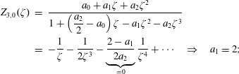 $$\begin{eqnarray}\displaystyle Z_{3,0}(\unicode[STIX]{x1D701}) & = & \displaystyle \frac{a_{0}+a_{1}\unicode[STIX]{x1D701}+a_{2}\unicode[STIX]{x1D701}^{2}}{1+\left({\displaystyle \frac{a_{2}}{2}}-a_{0}\right)\unicode[STIX]{x1D701}-a_{1}\unicode[STIX]{x1D701}^{2}-a_{2}\unicode[STIX]{x1D701}^{3}}\nonumber\\ \displaystyle & = & \displaystyle -\frac{1}{\unicode[STIX]{x1D701}}-\frac{1}{2\unicode[STIX]{x1D701}^{3}}-\underbrace{\frac{2-a_{1}}{2a_{2}}}_{=0}\frac{1}{\unicode[STIX]{x1D701}^{4}}+\cdots \quad \Rightarrow \quad a_{1}=2;\end{eqnarray}$$
 $$\begin{eqnarray}\displaystyle Z_{3,1}(\unicode[STIX]{x1D701}) & = & \displaystyle \frac{a_{0}+2\unicode[STIX]{x1D701}+a_{2}\unicode[STIX]{x1D701}^{2}}{1+\left({\displaystyle \frac{a_{2}}{2}}-a_{0}\right)\unicode[STIX]{x1D701}-2\unicode[STIX]{x1D701}^{2}-a_{2}\unicode[STIX]{x1D701}^{3}}\nonumber\\ \displaystyle & = & \displaystyle -\frac{1}{\unicode[STIX]{x1D701}}-\frac{1}{2\unicode[STIX]{x1D701}^{3}}-\underbrace{\frac{a_{2}-2a_{0}}{4a_{2}}}_{=3/4}\frac{1}{\unicode[STIX]{x1D701}^{5}}+\cdots \quad \Rightarrow \quad a_{2}=-a_{0};\end{eqnarray}$$
 $$\begin{eqnarray}\displaystyle Z_{3,2}(\unicode[STIX]{x1D701})=\frac{a_{0}+2\unicode[STIX]{x1D701}-a_{0}\unicode[STIX]{x1D701}^{2}}{1-\frac{3}{2}a_{0}\unicode[STIX]{x1D701}-2\unicode[STIX]{x1D701}^{2}+a_{0}\unicode[STIX]{x1D701}^{3}}. & & \displaystyle\end{eqnarray}$$
Matching these results with an expansion for small
 $\unicode[STIX]{x1D701}$
values is done according to
$\unicode[STIX]{x1D701}$
values is done according to
 $$\begin{eqnarray}\displaystyle & \displaystyle Z_{3,-2}(\unicode[STIX]{x1D701})=\frac{a_{0}+a_{1}\unicode[STIX]{x1D701}+a_{2}\unicode[STIX]{x1D701}^{2}}{1+b_{1}\unicode[STIX]{x1D701}+b_{2}\unicode[STIX]{x1D701}^{2}-a_{2}\unicode[STIX]{x1D701}^{3}}=i\sqrt{\unicode[STIX]{x03C0}}-2\unicode[STIX]{x1D701}-i\sqrt{\unicode[STIX]{x03C0}}\unicode[STIX]{x1D701}^{2}+\frac{4}{3}\unicode[STIX]{x1D701}^{3}+i\frac{\sqrt{\unicode[STIX]{x03C0}}}{2}\unicode[STIX]{x1D701}^{4}; & \displaystyle \nonumber\\ \displaystyle & & \displaystyle\end{eqnarray}$$
 $$\begin{eqnarray}\displaystyle & \displaystyle Z_{3,-1}(\unicode[STIX]{x1D701})=\frac{a_{0}+a_{1}\unicode[STIX]{x1D701}+a_{2}\unicode[STIX]{x1D701}^{2}}{1+b_{1}\unicode[STIX]{x1D701}-a_{1}\unicode[STIX]{x1D701}^{2}-a_{2}\unicode[STIX]{x1D701}^{3}}=i\sqrt{\unicode[STIX]{x03C0}}-2\unicode[STIX]{x1D701}-i\sqrt{\unicode[STIX]{x03C0}}\unicode[STIX]{x1D701}^{2}+\frac{4}{3}\unicode[STIX]{x1D701}^{3}; & \displaystyle\end{eqnarray}$$
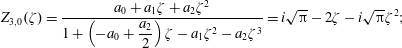 $$\begin{eqnarray}\displaystyle & \displaystyle Z_{3,0}(\unicode[STIX]{x1D701})=\frac{a_{0}+a_{1}\unicode[STIX]{x1D701}+a_{2}\unicode[STIX]{x1D701}^{2}}{1+\left(-a_{0}+{\displaystyle \frac{a_{2}}{2}}\right)\unicode[STIX]{x1D701}-a_{1}\unicode[STIX]{x1D701}^{2}-a_{2}\unicode[STIX]{x1D701}^{3}}=i\sqrt{\unicode[STIX]{x03C0}}-2\unicode[STIX]{x1D701}-i\sqrt{\unicode[STIX]{x03C0}}\unicode[STIX]{x1D701}^{2}; & \displaystyle\end{eqnarray}$$
 $$\begin{eqnarray}\displaystyle & \displaystyle Z_{3,1}(\unicode[STIX]{x1D701})=\frac{a_{0}+2\unicode[STIX]{x1D701}+a_{2}\unicode[STIX]{x1D701}^{2}}{1+\left({\displaystyle \frac{a_{2}}{2}}-a_{0}\right)\unicode[STIX]{x1D701}-2\unicode[STIX]{x1D701}^{2}-a_{2}\unicode[STIX]{x1D701}^{3}}=i\sqrt{\unicode[STIX]{x03C0}}-2\unicode[STIX]{x1D701}; & \displaystyle\end{eqnarray}$$
 $$\begin{eqnarray}\displaystyle & \displaystyle Z_{3,2}(\unicode[STIX]{x1D701})=\frac{a_{0}+2\unicode[STIX]{x1D701}-a_{0}\unicode[STIX]{x1D701}^{2}}{1-\frac{3}{2}a_{0}\unicode[STIX]{x1D701}-2\unicode[STIX]{x1D701}^{2}+a_{0}\unicode[STIX]{x1D701}^{3}}=i\sqrt{\unicode[STIX]{x03C0}}, & \displaystyle\end{eqnarray}$$
and the solutions are
 $$\begin{eqnarray}\displaystyle & \displaystyle Z_{3,-2}(\unicode[STIX]{x1D701})=\frac{i\sqrt{\unicode[STIX]{x03C0}}+{\displaystyle \frac{3\unicode[STIX]{x03C0}^{2}-30\unicode[STIX]{x03C0}+64}{2(5\unicode[STIX]{x03C0}-16)}}\unicode[STIX]{x1D701}+{\displaystyle \frac{i\sqrt{\unicode[STIX]{x03C0}}(9\unicode[STIX]{x03C0}-28)}{6(5\unicode[STIX]{x03C0}-16)}}\unicode[STIX]{x1D701}^{2}}{1-{\displaystyle \frac{i\sqrt{\unicode[STIX]{x03C0}}(3\unicode[STIX]{x03C0}-10)}{2(5\unicode[STIX]{x03C0}-16)}}\unicode[STIX]{x1D701}+{\displaystyle \frac{21\unicode[STIX]{x03C0}-64}{6(5\unicode[STIX]{x03C0}-16)}}\unicode[STIX]{x1D701}^{2}-{\displaystyle \frac{i\sqrt{\unicode[STIX]{x03C0}}(9\unicode[STIX]{x03C0}-28)}{6(5\unicode[STIX]{x03C0}-16)}}\unicode[STIX]{x1D701}^{3}}; & \displaystyle\end{eqnarray}$$
 $$\begin{eqnarray}\displaystyle & \displaystyle Z_{3,-1}(\unicode[STIX]{x1D701})=\frac{i\sqrt{\unicode[STIX]{x03C0}}+{\displaystyle \frac{10-3\unicode[STIX]{x03C0}}{3(\unicode[STIX]{x03C0}-3)}}\unicode[STIX]{x1D701}+{\displaystyle \frac{i(5\unicode[STIX]{x03C0}-16)}{3\sqrt{\unicode[STIX]{x03C0}}(\unicode[STIX]{x03C0}-3)}}\unicode[STIX]{x1D701}^{2}}{1-{\displaystyle \frac{i(3\unicode[STIX]{x03C0}-8)}{3\sqrt{\unicode[STIX]{x03C0}}(\unicode[STIX]{x03C0}-3)}}\unicode[STIX]{x1D701}-{\displaystyle \frac{10-3\unicode[STIX]{x03C0}}{3(\unicode[STIX]{x03C0}-3)}}\unicode[STIX]{x1D701}^{2}-{\displaystyle \frac{i(5\unicode[STIX]{x03C0}-16)}{3\sqrt{\unicode[STIX]{x03C0}}(\unicode[STIX]{x03C0}-3)}}\unicode[STIX]{x1D701}^{3}}; & \displaystyle\end{eqnarray}$$
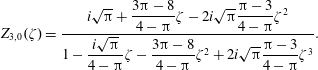 $$\begin{eqnarray}\displaystyle & \displaystyle Z_{3,0}(\unicode[STIX]{x1D701})=\frac{i\sqrt{\unicode[STIX]{x03C0}}+{\displaystyle \frac{3\unicode[STIX]{x03C0}-8}{4-\unicode[STIX]{x03C0}}}\unicode[STIX]{x1D701}-2i\sqrt{\unicode[STIX]{x03C0}}{\displaystyle \frac{\unicode[STIX]{x03C0}-3}{4-\unicode[STIX]{x03C0}}}\unicode[STIX]{x1D701}^{2}}{1-{\displaystyle \frac{i\sqrt{\unicode[STIX]{x03C0}}}{4-\unicode[STIX]{x03C0}}}\unicode[STIX]{x1D701}-{\displaystyle \frac{3\unicode[STIX]{x03C0}-8}{4-\unicode[STIX]{x03C0}}}\unicode[STIX]{x1D701}^{2}+2i\sqrt{\unicode[STIX]{x03C0}}{\displaystyle \frac{\unicode[STIX]{x03C0}-3}{4-\unicode[STIX]{x03C0}}}\unicode[STIX]{x1D701}^{3}}. & \displaystyle\end{eqnarray}$$
 $$\begin{eqnarray}\displaystyle & \displaystyle Z_{3,1}(\unicode[STIX]{x1D701})=\frac{i\sqrt{\unicode[STIX]{x03C0}}+2\unicode[STIX]{x1D701}-2i{\displaystyle \frac{4-\unicode[STIX]{x03C0}}{\sqrt{\unicode[STIX]{x03C0}}}}\unicode[STIX]{x1D701}^{2}}{1-i{\displaystyle \frac{4}{\sqrt{\unicode[STIX]{x03C0}}}}\unicode[STIX]{x1D701}-2\unicode[STIX]{x1D701}^{2}+2i{\displaystyle \frac{4-\unicode[STIX]{x03C0}}{\sqrt{\unicode[STIX]{x03C0}}}}\unicode[STIX]{x1D701}^{3}}; & \displaystyle\end{eqnarray}$$
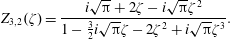 $$\begin{eqnarray}\displaystyle & \displaystyle Z_{3,2}(\unicode[STIX]{x1D701})=\frac{i\sqrt{\unicode[STIX]{x03C0}}+2\unicode[STIX]{x1D701}-i\sqrt{\unicode[STIX]{x03C0}}\unicode[STIX]{x1D701}^{2}}{1-\frac{3}{2}i\sqrt{\unicode[STIX]{x03C0}}\unicode[STIX]{x1D701}-2\unicode[STIX]{x1D701}^{2}+i\sqrt{\unicode[STIX]{x03C0}}\unicode[STIX]{x1D701}^{3}}. & \displaystyle\end{eqnarray}$$
Of course, the following relations now hold exactly
 $$\begin{eqnarray}\displaystyle & \displaystyle R_{3,0}(\unicode[STIX]{x1D701})=1+\unicode[STIX]{x1D701}Z_{3,0}(\unicode[STIX]{x1D701}); & \displaystyle\end{eqnarray}$$
 $$\begin{eqnarray}\displaystyle & \displaystyle R_{3,1}(\unicode[STIX]{x1D701})=1+\unicode[STIX]{x1D701}Z_{3,1}(\unicode[STIX]{x1D701}); & \displaystyle\end{eqnarray}$$
 $$\begin{eqnarray}\displaystyle & \displaystyle R_{3,2}(\unicode[STIX]{x1D701})=1+\unicode[STIX]{x1D701}Z_{3,2}(\unicode[STIX]{x1D701}). & \displaystyle\end{eqnarray}$$
3.3.3 Four-pole approximants of
$R(\unicode[STIX]{x1D701})$
and
$Z(\unicode[STIX]{x1D701})$


As before, the procedure of matching with asymptotic expansion yields (for simplicity already assuming
 $a_{0}=1$
)
$a_{0}=1$
)
 $$\begin{eqnarray}\frac{1+a_{1}\unicode[STIX]{x1D701}+a_{2}\unicode[STIX]{x1D701}^{2}}{1+b_{1}\unicode[STIX]{x1D701}+b_{2}\unicode[STIX]{x1D701}^{2}+b_{3}\unicode[STIX]{x1D701}^{3}+b_{4}\unicode[STIX]{x1D701}^{4}}=\underbrace{\frac{a_{2}}{b_{4}}}_{=-1/2}\frac{1}{\unicode[STIX]{x1D701}^{2}}+\cdots \quad \Rightarrow \quad b_{4}=-2a_{2};\end{eqnarray}$$
 $$\begin{eqnarray}\displaystyle R_{4,0}(\unicode[STIX]{x1D701}) & = & \displaystyle \frac{1+a_{1}\unicode[STIX]{x1D701}+a_{2}\unicode[STIX]{x1D701}^{2}}{1+b_{1}\unicode[STIX]{x1D701}+b_{2}\unicode[STIX]{x1D701}^{2}+b_{3}\unicode[STIX]{x1D701}^{3}-2a_{2}\unicode[STIX]{x1D701}^{4}}\nonumber\\ \displaystyle & = & \displaystyle -\frac{1}{2\unicode[STIX]{x1D701}^{2}}-\underbrace{\frac{a_{1}+{\displaystyle \frac{b_{3}}{2}}}{2a_{2}}}_{=0}\frac{1}{\unicode[STIX]{x1D701}^{3}}+\cdots \quad \Rightarrow \quad b_{3}=-2a_{1};\end{eqnarray}$$
 $$\begin{eqnarray}\displaystyle R_{4,1}(\unicode[STIX]{x1D701}) & = & \displaystyle \frac{1+a_{1}\unicode[STIX]{x1D701}+a_{2}\unicode[STIX]{x1D701}^{2}}{1+b_{1}\unicode[STIX]{x1D701}+b_{2}\unicode[STIX]{x1D701}^{2}-2a_{1}\unicode[STIX]{x1D701}^{3}-2a_{2}\unicode[STIX]{x1D701}^{4}}\nonumber\\ \displaystyle & = & \displaystyle -\frac{1}{2\unicode[STIX]{x1D701}^{2}}-\underbrace{\frac{1+{\displaystyle \frac{b_{2}}{2}}}{2a_{2}}}_{=3/4}\frac{1}{\unicode[STIX]{x1D701}^{4}}+\cdots \quad \Rightarrow \quad b_{2}=3a_{2}-2;\end{eqnarray}$$
 $$\begin{eqnarray}\displaystyle R_{4,2}(\unicode[STIX]{x1D701}) & = & \displaystyle \frac{1+a_{1}\unicode[STIX]{x1D701}+a_{2}\unicode[STIX]{x1D701}^{2}}{1+b_{1}\unicode[STIX]{x1D701}+(3a_{2}-2)\unicode[STIX]{x1D701}^{2}-2a_{1}\unicode[STIX]{x1D701}^{3}-2a_{2}\unicode[STIX]{x1D701}^{4}}\nonumber\\ \displaystyle & = & \displaystyle -\frac{1}{2\unicode[STIX]{x1D701}^{2}}-\frac{3}{4\unicode[STIX]{x1D701}^{4}}-\underbrace{\frac{b_{1}-3a_{1}}{4a_{2}}}_{=0}\frac{1}{\unicode[STIX]{x1D701}^{5}}+\cdots \quad \Rightarrow \quad b_{1}=3a_{1};\end{eqnarray}$$
 $$\begin{eqnarray}\displaystyle R_{4,3}(\unicode[STIX]{x1D701}) & = & \displaystyle \frac{1+a_{1}\unicode[STIX]{x1D701}+a_{2}\unicode[STIX]{x1D701}^{2}}{1+3a_{1}\unicode[STIX]{x1D701}+(3a_{2}-2)\unicode[STIX]{x1D701}^{2}-2a_{1}\unicode[STIX]{x1D701}^{3}-2a_{2}\unicode[STIX]{x1D701}^{4}}\nonumber\\ \displaystyle & = & \displaystyle -\frac{1}{2\unicode[STIX]{x1D701}^{2}}-\frac{3}{4\unicode[STIX]{x1D701}^{4}}-\underbrace{\frac{\frac{9}{2}a_{2}-2}{4a_{2}}}_{=15/8}\frac{1}{\unicode[STIX]{x1D701}^{6}}+\cdots \quad \Rightarrow \quad a_{2}=-\frac{2}{3};\end{eqnarray}$$
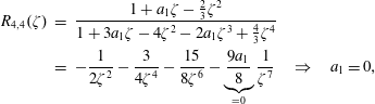 $$\begin{eqnarray}\displaystyle R_{4,4}(\unicode[STIX]{x1D701}) & = & \displaystyle \frac{1+a_{1}\unicode[STIX]{x1D701}-\frac{2}{3}\unicode[STIX]{x1D701}^{2}}{1+3a_{1}\unicode[STIX]{x1D701}-4\unicode[STIX]{x1D701}^{2}-2a_{1}\unicode[STIX]{x1D701}^{3}+\frac{4}{3}\unicode[STIX]{x1D701}^{4}}\nonumber\\ \displaystyle & = & \displaystyle -\frac{1}{2\unicode[STIX]{x1D701}^{2}}-\frac{3}{4\unicode[STIX]{x1D701}^{4}}-\frac{15}{8\unicode[STIX]{x1D701}^{6}}-\underbrace{\frac{9a_{1}}{8}}_{=0}\frac{1}{\unicode[STIX]{x1D701}^{7}}\quad \Rightarrow \quad a_{1}=0,\end{eqnarray}$$
where the last relation implies a possible approximant
 $R_{4,5}(\unicode[STIX]{x1D701})=(1-\frac{2}{3}\unicode[STIX]{x1D701}^{2})/(1-4\unicode[STIX]{x1D701}^{2}+\frac{4}{3}\unicode[STIX]{x1D701}^{4})$
. However, such an approximant is not well behaved (it has zero imaginary part for real valued
$R_{4,5}(\unicode[STIX]{x1D701})=(1-\frac{2}{3}\unicode[STIX]{x1D701}^{2})/(1-4\unicode[STIX]{x1D701}^{2}+\frac{4}{3}\unicode[STIX]{x1D701}^{4})$
. However, such an approximant is not well behaved (it has zero imaginary part for real valued
 $\unicode[STIX]{x1D701}$
) and the
$\unicode[STIX]{x1D701}$
) and the
 $R_{4,5}(\unicode[STIX]{x1D701})$
is eliminated. Matching with the power series is performed according to
$R_{4,5}(\unicode[STIX]{x1D701})$
is eliminated. Matching with the power series is performed according to
 $$\begin{eqnarray}\displaystyle R_{4,0}(\unicode[STIX]{x1D701}) & = & \displaystyle \frac{1+a_{1}\unicode[STIX]{x1D701}+a_{2}\unicode[STIX]{x1D701}^{2}}{1+b_{1}\unicode[STIX]{x1D701}+b_{2}\unicode[STIX]{x1D701}^{2}+b_{3}\unicode[STIX]{x1D701}^{3}-2a_{2}\unicode[STIX]{x1D701}^{4}}\nonumber\\ \displaystyle & = & \displaystyle 1+i\sqrt{\unicode[STIX]{x03C0}}\unicode[STIX]{x1D701}-2\unicode[STIX]{x1D701}^{2}-i\sqrt{\unicode[STIX]{x03C0}}\unicode[STIX]{x1D701}^{3}+\frac{4}{3}\unicode[STIX]{x1D701}^{4}+i\frac{\sqrt{\unicode[STIX]{x03C0}}}{2}\unicode[STIX]{x1D701}^{5};\end{eqnarray}$$
 $$\begin{eqnarray}R_{4,1}(\unicode[STIX]{x1D701})=\frac{1+a_{1}\unicode[STIX]{x1D701}+a_{2}\unicode[STIX]{x1D701}^{2}}{1+b_{1}\unicode[STIX]{x1D701}+b_{2}\unicode[STIX]{x1D701}^{2}-2a_{1}\unicode[STIX]{x1D701}^{3}-2a_{2}\unicode[STIX]{x1D701}^{4}}=1+i\sqrt{\unicode[STIX]{x03C0}}\unicode[STIX]{x1D701}-2\unicode[STIX]{x1D701}^{2}-i\sqrt{\unicode[STIX]{x03C0}}\unicode[STIX]{x1D701}^{3}+\frac{4}{3}\unicode[STIX]{x1D701}^{4};\end{eqnarray}$$
 $$\begin{eqnarray}R_{4,2}(\unicode[STIX]{x1D701})=\frac{1+a_{1}\unicode[STIX]{x1D701}+a_{2}\unicode[STIX]{x1D701}^{2}}{1+b_{1}\unicode[STIX]{x1D701}+(3a_{2}-2)\unicode[STIX]{x1D701}^{2}-2a_{1}\unicode[STIX]{x1D701}^{3}-2a_{2}\unicode[STIX]{x1D701}^{4}}=1+i\sqrt{\unicode[STIX]{x03C0}}\unicode[STIX]{x1D701}-2\unicode[STIX]{x1D701}^{2}-i\sqrt{\unicode[STIX]{x03C0}}\unicode[STIX]{x1D701}^{3};\end{eqnarray}$$
 $$\begin{eqnarray}\displaystyle & \displaystyle R_{4,3}(\unicode[STIX]{x1D701})=\frac{1+a_{1}\unicode[STIX]{x1D701}+a_{2}\unicode[STIX]{x1D701}^{2}}{1+3a_{1}\unicode[STIX]{x1D701}+(3a_{2}-2)\unicode[STIX]{x1D701}^{2}-2a_{1}\unicode[STIX]{x1D701}^{3}-2a_{2}\unicode[STIX]{x1D701}^{4}}=1+i\sqrt{\unicode[STIX]{x03C0}}\unicode[STIX]{x1D701}-2\unicode[STIX]{x1D701}^{2}; & \displaystyle\end{eqnarray}$$
 $$\begin{eqnarray}\displaystyle & \displaystyle R_{4,4}(\unicode[STIX]{x1D701})=\frac{1+a_{1}\unicode[STIX]{x1D701}-\frac{2}{3}\unicode[STIX]{x1D701}^{2}}{1+3a_{1}\unicode[STIX]{x1D701}-4\unicode[STIX]{x1D701}^{2}-2a_{1}\unicode[STIX]{x1D701}^{3}+\frac{4}{3}\unicode[STIX]{x1D701}^{4}}=1+i\sqrt{\unicode[STIX]{x03C0}}\unicode[STIX]{x1D701}, & \displaystyle\end{eqnarray}$$
and the results are
 $$\begin{eqnarray}\displaystyle & & \displaystyle R_{4,0}(\unicode[STIX]{x1D701})=\frac{1+i{\displaystyle \frac{\sqrt{\unicode[STIX]{x03C0}}}{2}}{\displaystyle \frac{(12\unicode[STIX]{x03C0}^{2}-67\unicode[STIX]{x03C0}+92)}{(6\unicode[STIX]{x03C0}^{2}-29\unicode[STIX]{x03C0}+32)}}\unicode[STIX]{x1D701}-{\displaystyle \frac{(9\unicode[STIX]{x03C0}^{2}-69\unicode[STIX]{x03C0}+128)}{6(6\unicode[STIX]{x03C0}^{2}-29\unicode[STIX]{x03C0}+32)}}\unicode[STIX]{x1D701}^{2}}{1-i{\displaystyle \frac{\sqrt{\unicode[STIX]{x03C0}}}{2}}{\displaystyle \frac{(9\unicode[STIX]{x03C0}-28)}{(6\unicode[STIX]{x03C0}^{2}-29\unicode[STIX]{x03C0}+32)}}\unicode[STIX]{x1D701}+{\displaystyle \frac{(36\unicode[STIX]{x03C0}^{2}-195\unicode[STIX]{x03C0}+256)}{6(6\unicode[STIX]{x03C0}^{2}-29\unicode[STIX]{x03C0}+32)}}\unicode[STIX]{x1D701}^{2}-i{\displaystyle \frac{\sqrt{\unicode[STIX]{x03C0}}(33\unicode[STIX]{x03C0}-104)}{6(6\unicode[STIX]{x03C0}^{2}-29\unicode[STIX]{x03C0}+32)}}\unicode[STIX]{x1D701}^{3}+{\displaystyle \frac{(9\unicode[STIX]{x03C0}^{2}-69\unicode[STIX]{x03C0}+128)}{3(6\unicode[STIX]{x03C0}^{2}-29\unicode[STIX]{x03C0}+32)}}\unicode[STIX]{x1D701}^{4}};\nonumber\\ \displaystyle & & \displaystyle\end{eqnarray}$$
 $$\begin{eqnarray}\displaystyle & & \displaystyle R_{4,1}(\unicode[STIX]{x1D701})=\frac{1-i{\displaystyle \frac{\sqrt{\unicode[STIX]{x03C0}}}{3}}{\displaystyle \frac{(9\unicode[STIX]{x03C0}-28)}{(16-5\unicode[STIX]{x03C0})}}\unicode[STIX]{x1D701}-{\displaystyle \frac{(6\unicode[STIX]{x03C0}^{2}-29\unicode[STIX]{x03C0}+32)}{3(16-5\unicode[STIX]{x03C0})}}\unicode[STIX]{x1D701}^{2}}{1-i{\displaystyle \frac{2\sqrt{\unicode[STIX]{x03C0}}}{3}}{\displaystyle \frac{(10-3\unicode[STIX]{x03C0})}{(16-5\unicode[STIX]{x03C0})}}\unicode[STIX]{x1D701}-{\displaystyle \frac{(21\unicode[STIX]{x03C0}-64)}{3(16-5\unicode[STIX]{x03C0})}}\unicode[STIX]{x1D701}^{2}+i{\displaystyle \frac{2\sqrt{\unicode[STIX]{x03C0}}}{3}}{\displaystyle \frac{(9\unicode[STIX]{x03C0}-28)}{(16-5\unicode[STIX]{x03C0})}}\unicode[STIX]{x1D701}^{3}+{\displaystyle \frac{2(6\unicode[STIX]{x03C0}^{2}-29\unicode[STIX]{x03C0}+32)}{3(16-5\unicode[STIX]{x03C0})}}\unicode[STIX]{x1D701}^{4}};\nonumber\\ \displaystyle & & \displaystyle\end{eqnarray}$$
 $$\begin{eqnarray}R_{4,2}(\unicode[STIX]{x1D701})=\frac{1-i\sqrt{\unicode[STIX]{x03C0}}{\displaystyle \frac{(10-3\unicode[STIX]{x03C0})}{(3\unicode[STIX]{x03C0}-8)}}\unicode[STIX]{x1D701}-{\displaystyle \frac{(16-5\unicode[STIX]{x03C0})}{(3\unicode[STIX]{x03C0}-8)}}\unicode[STIX]{x1D701}^{2}}{1-i\sqrt{\unicode[STIX]{x03C0}}{\displaystyle \frac{2}{(3\unicode[STIX]{x03C0}-8)}}\unicode[STIX]{x1D701}-{\displaystyle \frac{(32-9\unicode[STIX]{x03C0})}{(3\unicode[STIX]{x03C0}-8)}}\unicode[STIX]{x1D701}^{2}+i\sqrt{\unicode[STIX]{x03C0}}{\displaystyle \frac{2(10-3\unicode[STIX]{x03C0})}{(3\unicode[STIX]{x03C0}-8)}}\unicode[STIX]{x1D701}^{3}+{\displaystyle \frac{2(16-5\unicode[STIX]{x03C0})}{(3\unicode[STIX]{x03C0}-8)}}\unicode[STIX]{x1D701}^{4}}\end{eqnarray}$$
 $$\begin{eqnarray}\displaystyle & \displaystyle R_{4,3}(\unicode[STIX]{x1D701})=\frac{1-i{\displaystyle \frac{\sqrt{\unicode[STIX]{x03C0}}}{2}}\unicode[STIX]{x1D701}-{\displaystyle \frac{(3\unicode[STIX]{x03C0}-8)}{4}}\unicode[STIX]{x1D701}^{2}}{1-i{\displaystyle \frac{3\sqrt{\unicode[STIX]{x03C0}}}{2}}\unicode[STIX]{x1D701}-{\displaystyle \frac{(9\unicode[STIX]{x03C0}-16)}{4}}\unicode[STIX]{x1D701}^{2}+i\sqrt{\unicode[STIX]{x03C0}}\unicode[STIX]{x1D701}^{3}+{\displaystyle \frac{(3\unicode[STIX]{x03C0}-8)}{2}}\unicode[STIX]{x1D701}^{4}}; & \displaystyle\end{eqnarray}$$
 $$\begin{eqnarray}\displaystyle & \displaystyle R_{4,4}(\unicode[STIX]{x1D701})=\frac{1-i{\displaystyle \frac{\sqrt{\unicode[STIX]{x03C0}}}{2}}\unicode[STIX]{x1D701}-{\displaystyle \frac{2}{3}}\unicode[STIX]{x1D701}^{2}}{1-i{\displaystyle \frac{3\sqrt{\unicode[STIX]{x03C0}}}{2}}\unicode[STIX]{x1D701}-4\unicode[STIX]{x1D701}^{2}+i\sqrt{\unicode[STIX]{x03C0}}\unicode[STIX]{x1D701}^{3}+\frac{4}{3}\unicode[STIX]{x1D701}^{4}}. & \displaystyle\end{eqnarray}$$
Of the four-pole approximants, perhaps the most well-known one is
 $R_{4,3}(\unicode[STIX]{x1D701})$
used for example by Hammett & Perkins (Reference Hammett and Perkins1990), Passot & Sulem (Reference Passot and Sulem2007) etc., and which can be written in a convenient form
$R_{4,3}(\unicode[STIX]{x1D701})$
used for example by Hammett & Perkins (Reference Hammett and Perkins1990), Passot & Sulem (Reference Passot and Sulem2007) etc., and which can be written in a convenient form
Here we do not double check the derivation of the
 $Z_{4}(\unicode[STIX]{x1D701})$
approximants ‘from scratch’, and for a given
$Z_{4}(\unicode[STIX]{x1D701})$
approximants ‘from scratch’, and for a given
 $R_{4}$
coefficients, the
$R_{4}$
coefficients, the
 $Z_{4}$
coefficients are of course easily obtained by
$Z_{4}$
coefficients are of course easily obtained by
 $$\begin{eqnarray}R_{4}(\unicode[STIX]{x1D701})=\frac{1+a_{1}\unicode[STIX]{x1D701}+a_{2}\unicode[STIX]{x1D701}^{2}}{1+b_{1}\unicode[STIX]{x1D701}+b_{2}\unicode[STIX]{x1D701}^{2}+b_{3}\unicode[STIX]{x1D701}^{3}+b_{4}\unicode[STIX]{x1D701}^{4}}\quad \Rightarrow \quad Z_{4}(\unicode[STIX]{x1D701})=\frac{(a_{1}-b_{1})+(a_{2}-b_{2})\unicode[STIX]{x1D701}-b_{3}\unicode[STIX]{x1D701}^{2}-b_{4}\unicode[STIX]{x1D701}^{3}}{1+b_{1}\unicode[STIX]{x1D701}+b_{2}\unicode[STIX]{x1D701}^{2}+b_{3}\unicode[STIX]{x1D701}^{3}+b_{4}\unicode[STIX]{x1D701}^{4}}.\end{eqnarray}$$
For completeness, the corresponding results are
 $$\begin{eqnarray}\displaystyle Z_{4,0}(\unicode[STIX]{x1D701})=\frac{i\sqrt{\unicode[STIX]{x03C0}}-{\displaystyle \frac{(15\unicode[STIX]{x03C0}^{2}-88\unicode[STIX]{x03C0}+128)}{2(6\unicode[STIX]{x03C0}^{2}-29\unicode[STIX]{x03C0}+32)}}\unicode[STIX]{x1D701}+i{\displaystyle \frac{\sqrt{\unicode[STIX]{x03C0}}(33\unicode[STIX]{x03C0}-104)}{6(6\unicode[STIX]{x03C0}^{2}-29\unicode[STIX]{x03C0}+32)}}\unicode[STIX]{x1D701}^{2}-{\displaystyle \frac{(9\unicode[STIX]{x03C0}^{2}-69\unicode[STIX]{x03C0}+128)}{3(6\unicode[STIX]{x03C0}^{2}-29\unicode[STIX]{x03C0}+32)}}\unicode[STIX]{x1D701}^{3}}{1-i{\displaystyle \frac{\sqrt{\unicode[STIX]{x03C0}}}{2}}{\displaystyle \frac{(9\unicode[STIX]{x03C0}-28)}{(6\unicode[STIX]{x03C0}^{2}-29\unicode[STIX]{x03C0}+32)}}\unicode[STIX]{x1D701}+{\displaystyle \frac{(36\unicode[STIX]{x03C0}^{2}-195\unicode[STIX]{x03C0}+256)}{6(6\unicode[STIX]{x03C0}^{2}-29\unicode[STIX]{x03C0}+32)}}\unicode[STIX]{x1D701}^{2}-i{\displaystyle \frac{\sqrt{\unicode[STIX]{x03C0}}(33\unicode[STIX]{x03C0}-104)}{6(6\unicode[STIX]{x03C0}^{2}-29\unicode[STIX]{x03C0}+32)}}\unicode[STIX]{x1D701}^{3}+{\displaystyle \frac{(9\unicode[STIX]{x03C0}^{2}-69\unicode[STIX]{x03C0}+128)}{3(6\unicode[STIX]{x03C0}^{2}-29\unicode[STIX]{x03C0}+32)}}\unicode[STIX]{x1D701}^{4}}; & & \displaystyle \nonumber\\ \displaystyle & & \displaystyle\end{eqnarray}$$
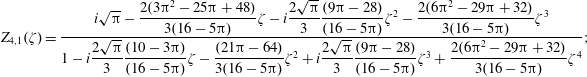 $$\begin{eqnarray}\displaystyle Z_{4,1}(\unicode[STIX]{x1D701})=\frac{i\sqrt{\unicode[STIX]{x03C0}}-{\displaystyle \frac{2(3\unicode[STIX]{x03C0}^{2}-25\unicode[STIX]{x03C0}+48)}{3(16-5\unicode[STIX]{x03C0})}}\unicode[STIX]{x1D701}-i{\displaystyle \frac{2\sqrt{\unicode[STIX]{x03C0}}}{3}}{\displaystyle \frac{(9\unicode[STIX]{x03C0}-28)}{(16-5\unicode[STIX]{x03C0})}}\unicode[STIX]{x1D701}^{2}-{\displaystyle \frac{2(6\unicode[STIX]{x03C0}^{2}-29\unicode[STIX]{x03C0}+32)}{3(16-5\unicode[STIX]{x03C0})}}\unicode[STIX]{x1D701}^{3}}{1-i{\displaystyle \frac{2\sqrt{\unicode[STIX]{x03C0}}}{3}}{\displaystyle \frac{(10-3\unicode[STIX]{x03C0})}{(16-5\unicode[STIX]{x03C0})}}\unicode[STIX]{x1D701}-{\displaystyle \frac{(21\unicode[STIX]{x03C0}-64)}{3(16-5\unicode[STIX]{x03C0})}}\unicode[STIX]{x1D701}^{2}+i{\displaystyle \frac{2\sqrt{\unicode[STIX]{x03C0}}}{3}}{\displaystyle \frac{(9\unicode[STIX]{x03C0}-28)}{(16-5\unicode[STIX]{x03C0})}}\unicode[STIX]{x1D701}^{3}+{\displaystyle \frac{2(6\unicode[STIX]{x03C0}^{2}-29\unicode[STIX]{x03C0}+32)}{3(16-5\unicode[STIX]{x03C0})}}\unicode[STIX]{x1D701}^{4}}; & & \displaystyle \nonumber\\ \displaystyle & & \displaystyle\end{eqnarray}$$
 $$\begin{eqnarray}\displaystyle & \displaystyle Z_{4,2}(\unicode[STIX]{x1D701})=\frac{i\sqrt{\unicode[STIX]{x03C0}}+{\displaystyle \frac{4(4-\unicode[STIX]{x03C0})}{(3\unicode[STIX]{x03C0}-8)}}\unicode[STIX]{x1D701}-i\sqrt{\unicode[STIX]{x03C0}}{\displaystyle \frac{2(10-3\unicode[STIX]{x03C0})}{(3\unicode[STIX]{x03C0}-8)}}\unicode[STIX]{x1D701}^{2}-{\displaystyle \frac{2(16-5\unicode[STIX]{x03C0})}{(3\unicode[STIX]{x03C0}-8)}}\unicode[STIX]{x1D701}^{3}}{1-i\sqrt{\unicode[STIX]{x03C0}}{\displaystyle \frac{2}{(3\unicode[STIX]{x03C0}-8)}}\unicode[STIX]{x1D701}-{\displaystyle \frac{(32-9\unicode[STIX]{x03C0})}{(3\unicode[STIX]{x03C0}-8)}}\unicode[STIX]{x1D701}^{2}+i\sqrt{\unicode[STIX]{x03C0}}{\displaystyle \frac{2(10-3\unicode[STIX]{x03C0})}{(3\unicode[STIX]{x03C0}-8)}}\unicode[STIX]{x1D701}^{3}+{\displaystyle \frac{2(16-5\unicode[STIX]{x03C0})}{(3\unicode[STIX]{x03C0}-8)}}\unicode[STIX]{x1D701}^{4}} & \displaystyle \nonumber\\ \displaystyle & & \displaystyle\end{eqnarray}$$
 $$\begin{eqnarray}\displaystyle & \displaystyle Z_{4,3}(\unicode[STIX]{x1D701})=\frac{i\sqrt{\unicode[STIX]{x03C0}}+{\displaystyle \frac{3\unicode[STIX]{x03C0}-4}{2}}\unicode[STIX]{x1D701}-i\sqrt{\unicode[STIX]{x03C0}}\unicode[STIX]{x1D701}^{2}-{\displaystyle \frac{(3\unicode[STIX]{x03C0}-8)}{2}}\unicode[STIX]{x1D701}^{3}}{1-i{\displaystyle \frac{3\sqrt{\unicode[STIX]{x03C0}}}{2}}\unicode[STIX]{x1D701}-{\displaystyle \frac{(9\unicode[STIX]{x03C0}-16)}{4}}\unicode[STIX]{x1D701}^{2}+i\sqrt{\unicode[STIX]{x03C0}}\unicode[STIX]{x1D701}^{3}+{\displaystyle \frac{(3\unicode[STIX]{x03C0}-8)}{2}}\unicode[STIX]{x1D701}^{4}}; & \displaystyle\end{eqnarray}$$
 $$\begin{eqnarray}\displaystyle & \displaystyle Z_{4,4}(\unicode[STIX]{x1D701})=\frac{i\sqrt{\unicode[STIX]{x03C0}}+\frac{10}{3}\unicode[STIX]{x1D701}-i\sqrt{\unicode[STIX]{x03C0}}\unicode[STIX]{x1D701}^{2}-\frac{4}{3}\unicode[STIX]{x1D701}^{3}}{1-i{\displaystyle \frac{3\sqrt{\unicode[STIX]{x03C0}}}{2}}\unicode[STIX]{x1D701}-4\unicode[STIX]{x1D701}^{2}+i\sqrt{\unicode[STIX]{x03C0}}\unicode[STIX]{x1D701}^{3}+\frac{4}{3}\unicode[STIX]{x1D701}^{4}}. & \displaystyle\end{eqnarray}$$
3.4 Conversion of our 2-index
$R_{n,n^{\prime }}(\unicode[STIX]{x1D701})$
notation to other notations

For clarity, we provide conversion tables of Padé approximants in the notation of Martín et al. (Reference Martín, Donoso and Zamudio-Cristi1980) and Hedrick & Leboeuf (Reference Hedrick and Leboeuf1992) to our notation. Comparing our analytic results to those of Martín et al. (Reference Martín, Donoso and Zamudio-Cristi1980) (introducing superscript
 $M$
), can be done easily according to
$M$
), can be done easily according to
 $$\begin{eqnarray}Z_{3,1}^{M}=Z_{2,-2};\quad Z_{2,2}^{M}=Z_{2,-1};\quad Z_{1,3}^{M}=Z_{2,0};\end{eqnarray}$$
 $$\begin{eqnarray}Z_{5,1}^{M}=Z_{3,-2};\quad Z_{4,2}^{M}=Z_{3,-1};\quad Z_{3,3}^{M}=Z_{3,0};\end{eqnarray}$$
 $$\begin{eqnarray}Z_{5,3}^{M}=Z_{4,0},\end{eqnarray}$$
and the general conversion can be written as
 $$\begin{eqnarray}Z_{n,n^{\prime }}^{M}=Z_{n+n^{\prime }/2,n^{\prime }-3}.\end{eqnarray}$$
The table 1 of Martín et al. (Reference Martín, Donoso and Zamudio-Cristi1980) can be now easily verified, which reveals a small obvious typo in their
 $Z_{4,2}^{M}$
, where the coefficient
$Z_{4,2}^{M}$
, where the coefficient
 $p_{2}$
is missing the imaginary i number.
$p_{2}$
is missing the imaginary i number.
To compare our results to those of Hedrick & Leboeuf (Reference Hedrick and Leboeuf1992), it is useful to calculate asymptotic expansions of their
 $Z_{n}$
definitions (that is defined as
$Z_{n}$
definitions (that is defined as
 $Z_{n,0}$
), that calculate as
$Z_{n,0}$
), that calculate as
 $$\begin{eqnarray}\displaystyle & \displaystyle Z_{2}^{HL}=-\frac{a_{1}-\unicode[STIX]{x1D701}}{a_{0}+a_{1}\unicode[STIX]{x1D701}-\unicode[STIX]{x1D701}^{2}}=-\frac{1}{\unicode[STIX]{x1D701}}-\frac{0}{\unicode[STIX]{x1D701}^{2}}+o\left(\frac{1}{\unicode[STIX]{x1D701}^{2}}\right); & \displaystyle\end{eqnarray}$$
 $$\begin{eqnarray}\displaystyle & \displaystyle Z_{3}^{HL}=-\frac{\unicode[STIX]{x1D701}^{2}-a_{2}\unicode[STIX]{x1D701}-a_{1}+\frac{1}{2}}{\unicode[STIX]{x1D701}^{3}-a_{2}\unicode[STIX]{x1D701}^{2}-a_{1}\unicode[STIX]{x1D701}-a_{0}}=-\frac{1}{\unicode[STIX]{x1D701}}-\frac{1}{2\unicode[STIX]{x1D701}^{3}}+o\left(\frac{1}{\unicode[STIX]{x1D701}^{3}}\right); & \displaystyle\end{eqnarray}$$
 $$\begin{eqnarray}\displaystyle & \displaystyle Z_{4}^{HL}=-\frac{\unicode[STIX]{x1D701}^{3}-a_{3}\unicode[STIX]{x1D701}^{2}-(a_{2}-\frac{1}{2}\unicode[STIX]{x1D701})-(a_{1}+a_{3}/2)}{\unicode[STIX]{x1D701}^{4}-a_{3}\unicode[STIX]{x1D701}^{3}-a_{2}\unicode[STIX]{x1D701}^{2}-a_{1}\unicode[STIX]{x1D701}-a_{0}}=-\frac{1}{\unicode[STIX]{x1D701}}-\frac{1}{2\unicode[STIX]{x1D701}^{3}}-\frac{0}{\unicode[STIX]{x1D701}^{4}}+o\left(\frac{1}{\unicode[STIX]{x1D701}^{4}}\right); & \displaystyle \nonumber\\ \displaystyle & & \displaystyle\end{eqnarray}$$
 $$\begin{eqnarray}\displaystyle Z_{5}^{HL} & = & \displaystyle -\frac{\unicode[STIX]{x1D701}^{4}-a_{4}\unicode[STIX]{x1D701}^{3}-(a_{3}-\frac{1}{2})\unicode[STIX]{x1D701}^{2}-(a_{2}+a_{4}/2)\unicode[STIX]{x1D701}-(a_{1}+a_{3}/2-\frac{3}{4})}{\unicode[STIX]{x1D701}^{5}-a_{4}\unicode[STIX]{x1D701}^{4}-a_{3}\unicode[STIX]{x1D701}^{3}-a_{2}\unicode[STIX]{x1D701}^{2}-a_{1}\unicode[STIX]{x1D701}-a_{0}}\nonumber\\ \displaystyle & = & \displaystyle -\frac{1}{\unicode[STIX]{x1D701}}-\frac{1}{2\unicode[STIX]{x1D701}^{3}}-\frac{3}{4\unicode[STIX]{x1D701}^{5}}+o\left(\frac{1}{\unicode[STIX]{x1D701}^{5}}\right),\end{eqnarray}$$
where ‘
 $HL$
’ stands for Hedrick & Leboeuf (Reference Hedrick and Leboeuf1992). As one can see, the number of asymptotic points used in their basic definition of
$HL$
’ stands for Hedrick & Leboeuf (Reference Hedrick and Leboeuf1992). As one can see, the number of asymptotic points used in their basic definition of
 $Z_{n}$
, increases with the number of poles
$Z_{n}$
, increases with the number of poles
 $n$
. Compared to our definition, their
$n$
. Compared to our definition, their
 $Z_{2,0}$
is defined as having another asymptotic point (for a total of 2),
$Z_{2,0}$
is defined as having another asymptotic point (for a total of 2),
 $Z_{3,0}$
has another asymptotic point (for a total of 3),
$Z_{3,0}$
has another asymptotic point (for a total of 3),
 $Z_{4,0}$
another one (for a total of 4), and so on. Essentially, in their notation the basic
$Z_{4,0}$
another one (for a total of 4), and so on. Essentially, in their notation the basic
 $Z_{n,0}$
is defined as having ‘
$Z_{n,0}$
is defined as having ‘
 $n$
’ asymptotic points, and asymptotic precision
$n$
’ asymptotic points, and asymptotic precision
 $o(1/\unicode[STIX]{x1D701}^{n})$
. The conversion between their and our notation is easy, and
$o(1/\unicode[STIX]{x1D701}^{n})$
. The conversion between their and our notation is easy, and
 $$\begin{eqnarray}\displaystyle Z_{2,0}^{HL} & = & \displaystyle Z_{2,-1};\quad Z_{2,1}^{HL}=Z_{2,0};\end{eqnarray}$$
 $$\begin{eqnarray}\displaystyle Z_{3,1}^{HL} & = & \displaystyle Z_{3,1};\quad Z_{3,2}^{HL}=Z_{3,2};\end{eqnarray}$$
 $$\begin{eqnarray}\displaystyle Z_{4,1}^{HL} & = & \displaystyle Z_{4,2};\quad Z_{4,2}^{HL}=Z_{4,3};\quad Z_{4,3}^{HL}=Z_{4,4};\end{eqnarray}$$
 $$\begin{eqnarray}\displaystyle Z_{5,1}^{HL} & = & \displaystyle Z_{5,3};\quad Z_{5,2}^{HL}=Z_{5,4};\quad Z_{5,3}^{HL}=Z_{5,5};\quad Z_{5,4}^{HL}=Z_{5,6},\end{eqnarray}$$
or the general conversion can be written as
 $$\begin{eqnarray}Z_{n,n^{\prime }}^{HL}=Z_{n,n^{\prime }+n-3}.\end{eqnarray}$$
We checked the table 1 of Hedrick & Leboeuf (Reference Hedrick and Leboeuf1992) that provides coefficients for the Padé approximants (3.183)–(3.186) and we can confirm that the table is essentially correct, except for one coefficient.Footnote
7
The coefficient where a simple typo is suspected is the coefficient
 $a_{1}$
in
$a_{1}$
in
 $Z_{3,1}$
. Rewriting our three-pole approximant
$Z_{3,1}$
. Rewriting our three-pole approximant
 $R_{3}(\unicode[STIX]{x1D701})$
to the form used by Passot & Sulem (Reference Passot and Sulem2007) and Hedrick & Leboeuf (Reference Hedrick and Leboeuf1992) (that corresponds to the
$R_{3}(\unicode[STIX]{x1D701})$
to the form used by Passot & Sulem (Reference Passot and Sulem2007) and Hedrick & Leboeuf (Reference Hedrick and Leboeuf1992) (that corresponds to the
 $Z_{3}^{HL}$
as written in (3.180)) yields
$Z_{3}^{HL}$
as written in (3.180)) yields
 $$\begin{eqnarray}R_{3}(\unicode[STIX]{x1D701})=\frac{-\frac{1}{2}\unicode[STIX]{x1D701}-a_{0}}{\unicode[STIX]{x1D701}^{3}-a_{2}\unicode[STIX]{x1D701}^{2}-a_{1}\unicode[STIX]{x1D701}-a_{0}},\end{eqnarray}$$
which further yields
 $$\begin{eqnarray}\displaystyle & \displaystyle R_{3,1}(\unicode[STIX]{x1D701})=\frac{-{\displaystyle \frac{1}{2}}\unicode[STIX]{x1D701}-{\displaystyle \frac{i\sqrt{\unicode[STIX]{x03C0}}}{2(4-\unicode[STIX]{x03C0})}}}{\unicode[STIX]{x1D701}^{3}+{\displaystyle \frac{i\sqrt{\unicode[STIX]{x03C0}}}{(4-\unicode[STIX]{x03C0})}}\unicode[STIX]{x1D701}^{2}-{\displaystyle \frac{2}{(4-\unicode[STIX]{x03C0})}}\unicode[STIX]{x1D701}-{\displaystyle \frac{i\sqrt{\unicode[STIX]{x03C0}}}{2(4-\unicode[STIX]{x03C0})}}}; & \displaystyle\end{eqnarray}$$
 $$\begin{eqnarray}\displaystyle & \displaystyle R_{3,2}(\unicode[STIX]{x1D701})=\frac{-{\displaystyle \frac{1}{2}}\unicode[STIX]{x1D701}-{\displaystyle \frac{i}{\sqrt{\unicode[STIX]{x03C0}}}}}{\unicode[STIX]{x1D701}^{3}+{\displaystyle \frac{2i}{\sqrt{\unicode[STIX]{x03C0}}}}\unicode[STIX]{x1D701}^{2}-{\displaystyle \frac{3}{2}}\unicode[STIX]{x1D701}-{\displaystyle \frac{i}{\sqrt{\unicode[STIX]{x03C0}}}}}, & \displaystyle\end{eqnarray}$$
and our approximants are
 $$\begin{eqnarray}\displaystyle R_{3,1}(\unicode[STIX]{x1D701}):\quad a_{0} & = & \displaystyle \frac{i\sqrt{\unicode[STIX]{x03C0}}}{2(4-\unicode[STIX]{x03C0})}=1.03241i;\quad a_{1}=\frac{2}{4-\unicode[STIX]{x03C0}}=2.32990;\nonumber\\ \displaystyle a_{2} & = & \displaystyle -\frac{i\sqrt{\unicode[STIX]{x03C0}}}{4-\unicode[STIX]{x03C0}}=-2.06482i;\end{eqnarray}$$
 $$\begin{eqnarray}\displaystyle R_{3,2}(\unicode[STIX]{x1D701}):\quad a_{0} & = & \displaystyle \frac{i}{\sqrt{\unicode[STIX]{x03C0}}}=0.56419i;\quad a_{1}=\frac{3}{2};\nonumber\\ \displaystyle a_{2} & = & \displaystyle -\frac{2i}{\sqrt{\unicode[STIX]{x03C0}}}=-1.12838i.\end{eqnarray}$$
For the
 $a_{1}$
coefficient in
$a_{1}$
coefficient in
 $R_{3,1}$
, both Hedrick & Leboeuf (Reference Hedrick and Leboeuf1992) and Passot & Sulem (Reference Passot and Sulem2007) use
$R_{3,1}$
, both Hedrick & Leboeuf (Reference Hedrick and Leboeuf1992) and Passot & Sulem (Reference Passot and Sulem2007) use
 $a_{1}=2.23990$
instead of the correct
$a_{1}=2.23990$
instead of the correct
 $a_{1}=2.32990$
. The differences are of course small. Nevertheless, the new correct value explains the observation made by Passot & Sulem (Reference Passot and Sulem2007), in the paragraph below their figure 1, where they write: ‘It is conspicuous that
$a_{1}=2.32990$
. The differences are of course small. Nevertheless, the new correct value explains the observation made by Passot & Sulem (Reference Passot and Sulem2007), in the paragraph below their figure 1, where they write: ‘It is conspicuous that
 $R_{3,2}$
provides a fit that is slightly better for small
$R_{3,2}$
provides a fit that is slightly better for small
 $\unicode[STIX]{x1D701}$
, but turns out to be globally less accurate than
$\unicode[STIX]{x1D701}$
, but turns out to be globally less accurate than
 $R_{3,1}$
’. The authors obviously noticed that something is not right, since for small
$R_{3,1}$
’. The authors obviously noticed that something is not right, since for small
 $\unicode[STIX]{x1D701}$
, the
$\unicode[STIX]{x1D701}$
, the
 $R_{3,1}$
has precision
$R_{3,1}$
has precision
 $o(\unicode[STIX]{x1D701}^{2})$
and
$o(\unicode[STIX]{x1D701}^{2})$
and
 $R_{3,2}$
only
$R_{3,2}$
only
 $o(\unicode[STIX]{x1D701})$
, so the
$o(\unicode[STIX]{x1D701})$
, so the
 $R_{3,1}$
should be more precise. And it indeed is, the authors were just misguided by the wrong value of
$R_{3,1}$
should be more precise. And it indeed is, the authors were just misguided by the wrong value of
 $a_{1}$
introduced by Hedrick & Leboeuf (Reference Hedrick and Leboeuf1992).
$a_{1}$
introduced by Hedrick & Leboeuf (Reference Hedrick and Leboeuf1992).
3.5 Precision of
$R(\unicode[STIX]{x1D701})$
approximants

It is useful to compare the Padé approximants to the exact
 $R(\unicode[STIX]{x1D701})=1+\unicode[STIX]{x1D701}Z(\unicode[STIX]{x1D701})$
, where the plasma dispersion function can be conveniently calculated (for example in Maple) according to
$R(\unicode[STIX]{x1D701})=1+\unicode[STIX]{x1D701}Z(\unicode[STIX]{x1D701})$
, where the plasma dispersion function can be conveniently calculated (for example in Maple) according to
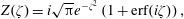 $$\begin{eqnarray}\displaystyle Z(\unicode[STIX]{x1D701})=i\sqrt{\unicode[STIX]{x03C0}}e^{-\unicode[STIX]{x1D701}^{2}}\left(1+\text{erf}(i\unicode[STIX]{x1D701})\right), & & \displaystyle\end{eqnarray}$$
where
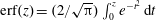 $\text{erf}(z)=(2/\sqrt{\unicode[STIX]{x03C0}})\int _{0}^{z}e^{-t^{2}}\,\text{d}t$
is the well-known error function, defined for any complex
$\text{erf}(z)=(2/\sqrt{\unicode[STIX]{x03C0}})\int _{0}^{z}e^{-t^{2}}\,\text{d}t$
is the well-known error function, defined for any complex
 $z$
. We plot only approximants for which we were able to obtain closures. The exact
$z$
. We plot only approximants for which we were able to obtain closures. The exact
 $R(\unicode[STIX]{x1D701})$
is plotted as a black solid line in all the figures. Figure 2 top shows one-pole and two-pole approximants
$R(\unicode[STIX]{x1D701})$
is plotted as a black solid line in all the figures. Figure 2 top shows one-pole and two-pole approximants
 $R_{1}(\unicode[STIX]{x1D701})$
(red dashed line) and
$R_{1}(\unicode[STIX]{x1D701})$
(red dashed line) and
 $R_{2,0}(\unicode[STIX]{x1D701})$
(blue dot-dashed line). Figure 2 bottom shows three-pole approximants
$R_{2,0}(\unicode[STIX]{x1D701})$
(blue dot-dashed line). Figure 2 bottom shows three-pole approximants
 $R_{3,0}(\unicode[STIX]{x1D701})$
(red dashed line),
$R_{3,0}(\unicode[STIX]{x1D701})$
(red dashed line),
 $R_{3,1}(\unicode[STIX]{x1D701})$
(green dotted line) and
$R_{3,1}(\unicode[STIX]{x1D701})$
(green dotted line) and
 $R_{3,2}(\unicode[STIX]{x1D701})$
(blue dot-dashed line). Figures in the left column show the imaginary part and figures in the right column show the real part. The input variable
$R_{3,2}(\unicode[STIX]{x1D701})$
(blue dot-dashed line). Figures in the left column show the imaginary part and figures in the right column show the real part. The input variable
 $\unicode[STIX]{x1D701}$
plotted on the
$\unicode[STIX]{x1D701}$
plotted on the
 $x$
-axis is prescribed to be real, i.e. states in the weak growth-rate/damping approximation are explored (one might as well prescribe
$x$
-axis is prescribed to be real, i.e. states in the weak growth-rate/damping approximation are explored (one might as well prescribe
 $\text{Im}(\unicode[STIX]{x1D701})=\pm 0.01\text{Re}(\unicode[STIX]{x1D701})$
and plot essentially the same graphs, with only small differences in solutions).
$\text{Im}(\unicode[STIX]{x1D701})=\pm 0.01\text{Re}(\unicode[STIX]{x1D701})$
and plot essentially the same graphs, with only small differences in solutions).
Figure 2. One-pole, two-pole (a,b) and three-pole (c,d) Padé approximants of
 $R(\unicode[STIX]{x1D701})$
. (a,c)
$R(\unicode[STIX]{x1D701})$
. (a,c)
 $\text{Im}R(\unicode[STIX]{x1D701})$
, (b,d)
$\text{Im}R(\unicode[STIX]{x1D701})$
, (b,d)
 $\text{Re}R(\unicode[STIX]{x1D701})$
, for
$\text{Re}R(\unicode[STIX]{x1D701})$
, for
 $\unicode[STIX]{x1D701}$
being real.
$\unicode[STIX]{x1D701}$
being real.
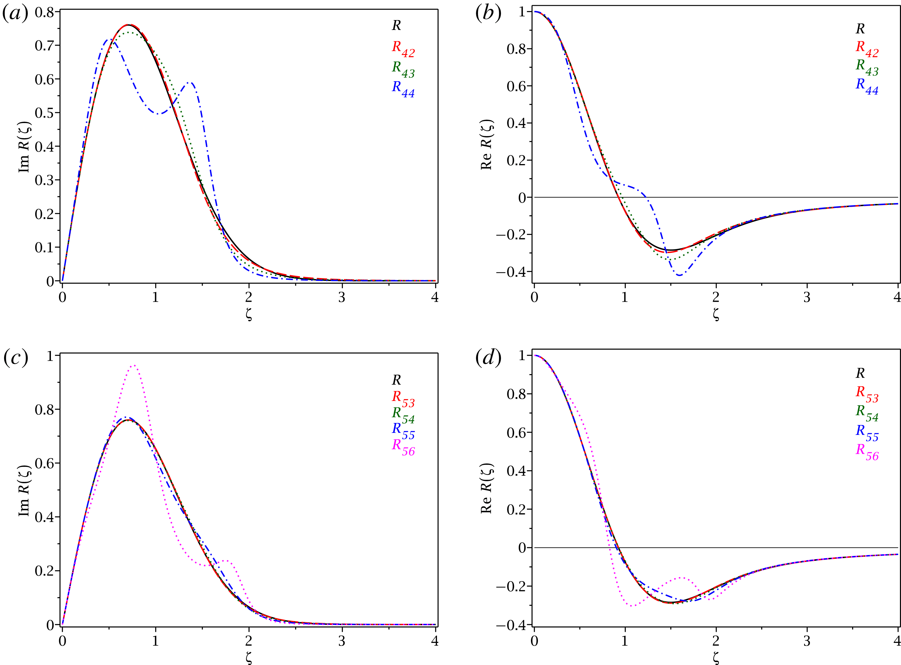
Figure 3. Four-pole (a,b) and five-pole (c,d) Padé approximants of
 $R(\unicode[STIX]{x1D701})$
.
$R(\unicode[STIX]{x1D701})$
.
As expected, the very simple approximant
 $R_{1}(\unicode[STIX]{x1D701})$
is unprecise for larger values of
$R_{1}(\unicode[STIX]{x1D701})$
is unprecise for larger values of
 $\unicode[STIX]{x1D701}$
, and above
$\unicode[STIX]{x1D701}$
, and above
 $\unicode[STIX]{x1D701}>1$
, the
$\unicode[STIX]{x1D701}>1$
, the
 $\text{Re}R_{1}(\unicode[STIX]{x1D701})$
even has a wrong sign. Nevertheless, the approximant is still a good approximant for small
$\text{Re}R_{1}(\unicode[STIX]{x1D701})$
even has a wrong sign. Nevertheless, the approximant is still a good approximant for small
 $\unicode[STIX]{x1D701}\ll 1$
values, and it is also very valuable from a theoretical perspective, since it is the only approximant that provides a quasi-static closure for the perpendicular heat flux
$\unicode[STIX]{x1D701}\ll 1$
values, and it is also very valuable from a theoretical perspective, since it is the only approximant that provides a quasi-static closure for the perpendicular heat flux
 $q_{\bot }$
(see the 3-D geometry § 4, closure (4.108)). This has one important implication:
$q_{\bot }$
(see the 3-D geometry § 4, closure (4.108)). This has one important implication:
If one renders the approximant
 $R_{1}$
as not satisfactory (which is true unless
$R_{1}$
as not satisfactory (which is true unless
 $\unicode[STIX]{x1D701}\ll 1$
or at least
$\unicode[STIX]{x1D701}\ll 1$
or at least
 $\unicode[STIX]{x1D701}<1$
), 3-D simulations with fluid models that contain Landau damping can be only performed with time-dependent heat flux equations. All other approximants in figure 2 perform reasonably well, and the most precise is
$\unicode[STIX]{x1D701}<1$
), 3-D simulations with fluid models that contain Landau damping can be only performed with time-dependent heat flux equations. All other approximants in figure 2 perform reasonably well, and the most precise is
 $R_{3,0}(\unicode[STIX]{x1D701})$
, followed by
$R_{3,0}(\unicode[STIX]{x1D701})$
, followed by
 $R_{3,1}(\unicode[STIX]{x1D701})$
.
$R_{3,1}(\unicode[STIX]{x1D701})$
.
Figure 3 shows selected four-pole and five-pole approximants for which we were able to obtain closures. Unfortunately, approximants
 $R_{4,4}(\unicode[STIX]{x1D701})$
and
$R_{4,4}(\unicode[STIX]{x1D701})$
and
 $R_{5,6}(\unicode[STIX]{x1D701})$
show a bit unpleasant behaviour, and the associated closures obtained with these approximants are therefore difficult to recommend, unless the considered domain is
$R_{5,6}(\unicode[STIX]{x1D701})$
show a bit unpleasant behaviour, and the associated closures obtained with these approximants are therefore difficult to recommend, unless the considered domain is
 $\unicode[STIX]{x1D701}\ll 1$
or
$\unicode[STIX]{x1D701}\ll 1$
or
 $\unicode[STIX]{x1D701}\gg 1$
, or more specifically, at least
$\unicode[STIX]{x1D701}\gg 1$
, or more specifically, at least
 $\unicode[STIX]{x1D701}<0.5$
or
$\unicode[STIX]{x1D701}<0.5$
or
 $\unicode[STIX]{x1D701}>2$
. The behaviour is not surprising, since approximants
$\unicode[STIX]{x1D701}>2$
. The behaviour is not surprising, since approximants
 $R_{4,4}(\unicode[STIX]{x1D701})$
and
$R_{4,4}(\unicode[STIX]{x1D701})$
and
 $R_{5,6}(\unicode[STIX]{x1D701})$
have the maximum available number of poles devoted to the asymptotic expansion
$R_{5,6}(\unicode[STIX]{x1D701})$
have the maximum available number of poles devoted to the asymptotic expansion
 $\unicode[STIX]{x1D701}\gg 1$
, without being ill posed. The closures are therefore specifically suitable for
$\unicode[STIX]{x1D701}\gg 1$
, without being ill posed. The closures are therefore specifically suitable for
 $\unicode[STIX]{x1D701}\gg 1$
regime, for example in the low-temperature limit, or, in the high-frequency (actually high phase speed) limit (since
$\unicode[STIX]{x1D701}\gg 1$
regime, for example in the low-temperature limit, or, in the high-frequency (actually high phase speed) limit (since
 $\unicode[STIX]{x1D701}=\unicode[STIX]{x1D714}/(|k_{\Vert }|v_{\text{th}\Vert })$
). For
$\unicode[STIX]{x1D701}=\unicode[STIX]{x1D714}/(|k_{\Vert }|v_{\text{th}\Vert })$
). For
 $R_{4,4}(\unicode[STIX]{x1D701})$
, the corresponding closures are the quasi-static closure (3.268) and time-dependent closures (3.295), (3.297), (3.299). For
$R_{4,4}(\unicode[STIX]{x1D701})$
, the corresponding closures are the quasi-static closure (3.268) and time-dependent closures (3.295), (3.297), (3.299). For
 $R_{5,6}(\unicode[STIX]{x1D701})$
, the corresponding closure is time dependent (3.325) and naturally, this is the most precise closure in the
$R_{5,6}(\unicode[STIX]{x1D701})$
, the corresponding closure is time dependent (3.325) and naturally, this is the most precise closure in the
 $\unicode[STIX]{x1D701}\gg 1$
regime, with precision
$\unicode[STIX]{x1D701}\gg 1$
regime, with precision
 $o(\unicode[STIX]{x1D701}^{-8})$
. Noticeably, the asymptotic precision is even better than the
$o(\unicode[STIX]{x1D701}^{-8})$
. Noticeably, the asymptotic precision is even better than the
 $R_{8,3}(\unicode[STIX]{x1D701})$
approximant used in the WHAMP code, which has a precision
$R_{8,3}(\unicode[STIX]{x1D701})$
approximant used in the WHAMP code, which has a precision
 $o(\unicode[STIX]{x1D701}^{-5})$
.
$o(\unicode[STIX]{x1D701}^{-5})$
.
All other approximants in figure 3 are very precise in the entire considered range of
 $\unicode[STIX]{x1D701}$
. To clearly see the precision, it is useful to calculate the maximum relative errors
$\unicode[STIX]{x1D701}$
. To clearly see the precision, it is useful to calculate the maximum relative errors
 $$\begin{eqnarray}\text{Im}\left(\frac{R_{n,n^{\prime }}(\unicode[STIX]{x1D701})-R(\unicode[STIX]{x1D701})}{R(\unicode[STIX]{x1D701})}\right)100\,\%;\quad \text{Re}\left(\frac{R_{n,n^{\prime }}(\unicode[STIX]{x1D701})-R(\unicode[STIX]{x1D701})}{R(\unicode[STIX]{x1D701})}\right)100\,\%,\end{eqnarray}$$
which we define this way instead of for example
 $\text{Re}(R_{n,n^{\prime }}(\unicode[STIX]{x1D701})-R(\unicode[STIX]{x1D701}))/\text{Re}R(\unicode[STIX]{x1D701})$
, since the real part of
$\text{Re}(R_{n,n^{\prime }}(\unicode[STIX]{x1D701})-R(\unicode[STIX]{x1D701}))/\text{Re}R(\unicode[STIX]{x1D701})$
, since the real part of
 $R(\unicode[STIX]{x1D701})$
is going through zero. The maximum relative errors typically appear for
$R(\unicode[STIX]{x1D701})$
is going through zero. The maximum relative errors typically appear for
 $\unicode[STIX]{x1D701}\in (0,4)$
, even though some reported values are outside of this range. The
$\unicode[STIX]{x1D701}\in (0,4)$
, even though some reported values are outside of this range. The
 $R_{1}(\unicode[STIX]{x1D701})$
approximant is excluded from the table since its relative error of the imaginary part increases with
$R_{1}(\unicode[STIX]{x1D701})$
approximant is excluded from the table since its relative error of the imaginary part increases with
 $\unicode[STIX]{x1D701}$
. We omit if errors are positive or negative and the results are:
$\unicode[STIX]{x1D701}$
. We omit if errors are positive or negative and the results are:

The numbers of course do not reveal the entire story, since the maximum error can occur for different
 $\unicode[STIX]{x1D701}$
values. For example, from the plots of
$\unicode[STIX]{x1D701}$
values. For example, from the plots of
 $\text{Im}R(\unicode[STIX]{x1D701})$
in figure 2, the approximant
$\text{Im}R(\unicode[STIX]{x1D701})$
in figure 2, the approximant
 $R_{3,0}(\unicode[STIX]{x1D701})$
captures the maximum (the peak around
$R_{3,0}(\unicode[STIX]{x1D701})$
captures the maximum (the peak around
 $\unicode[STIX]{x1D701}\sim 1$
) with much better accuracy than the approximant
$\unicode[STIX]{x1D701}\sim 1$
) with much better accuracy than the approximant
 $R_{3,1}(\unicode[STIX]{x1D701})$
. However, according to the above table, the
$R_{3,1}(\unicode[STIX]{x1D701})$
. However, according to the above table, the
 $R_{3,1}(\unicode[STIX]{x1D701})$
appears to be more precise globally. The discrepancy is easily understood from figure 4, where
$R_{3,1}(\unicode[STIX]{x1D701})$
appears to be more precise globally. The discrepancy is easily understood from figure 4, where
 $\%$
errors of both approximants are plotted with respect to
$\%$
errors of both approximants are plotted with respect to
 $\unicode[STIX]{x1D701}$
. A similar table and figures can be created for the heavily damped regime, for example for
$\unicode[STIX]{x1D701}$
. A similar table and figures can be created for the heavily damped regime, for example for
 $\unicode[STIX]{x1D701}$
with the imaginary part
$\unicode[STIX]{x1D701}$
with the imaginary part
 $\text{Im}(\unicode[STIX]{x1D701})=-\text{Re}(\unicode[STIX]{x1D701})/2$
, where the Padé approximants are less precise.
$\text{Im}(\unicode[STIX]{x1D701})=-\text{Re}(\unicode[STIX]{x1D701})/2$
, where the Padé approximants are less precise.
3.6 Landau fluid closures – fascinating closures for all
$\unicode[STIX]{x1D701}$

Now, let us use various Padé approximations of the plasma response function
 $R(\unicode[STIX]{x1D701})$
, and calculate the kinetic moments. Let us start with the simplest choice of replacing the exact
$R(\unicode[STIX]{x1D701})$
, and calculate the kinetic moments. Let us start with the simplest choice of replacing the exact
 $R(\unicode[STIX]{x1D701})$
with approximant
$R(\unicode[STIX]{x1D701})$
with approximant
 $R_{1}(\unicode[STIX]{x1D701})=1/(1-i\sqrt{\unicode[STIX]{x03C0}}\unicode[STIX]{x1D701})$
. Let us drop the index
$R_{1}(\unicode[STIX]{x1D701})=1/(1-i\sqrt{\unicode[STIX]{x03C0}}\unicode[STIX]{x1D701})$
. Let us drop the index
 $r$
. The linear kinetic moments (3.20)–(3.26) calculate as
$r$
. The linear kinetic moments (3.20)–(3.26) calculate as
 $$\begin{eqnarray}\displaystyle R_{1}(\unicode[STIX]{x1D701}):\quad \frac{n^{(1)}}{n_{0}} & = & \displaystyle -\frac{q_{r}}{T^{(0)}}\unicode[STIX]{x1D6F7}\frac{1}{1-i\sqrt{\unicode[STIX]{x03C0}}\unicode[STIX]{x1D701}}\left[1\right];\end{eqnarray}$$
 $$\begin{eqnarray}\displaystyle u^{(1)} & = & \displaystyle -\frac{q_{r}}{T^{(0)}}\unicode[STIX]{x1D6F7}v_{\text{th}}\text{sign}(k_{\Vert })\frac{1}{1-i\sqrt{\unicode[STIX]{x03C0}}\unicode[STIX]{x1D701}}\left[\unicode[STIX]{x1D701}\right];\end{eqnarray}$$
 $$\begin{eqnarray}\displaystyle \frac{p^{(1)}}{p_{0}} & = & \displaystyle -\frac{q_{r}}{T^{(0)}}\unicode[STIX]{x1D6F7}\frac{1}{1-i\sqrt{\unicode[STIX]{x03C0}}\unicode[STIX]{x1D701}}\left[2\unicode[STIX]{x1D701}^{2}-i\sqrt{\unicode[STIX]{x03C0}}\unicode[STIX]{x1D701}+1\right];\end{eqnarray}$$
 $$\begin{eqnarray}\displaystyle T^{(1)} & = & \displaystyle -q_{r}\unicode[STIX]{x1D6F7}\frac{1}{1-i\sqrt{\unicode[STIX]{x03C0}}\unicode[STIX]{x1D701}}\left[2\unicode[STIX]{x1D701}^{2}-i\sqrt{\unicode[STIX]{x03C0}}\unicode[STIX]{x1D701}\right];\end{eqnarray}$$
 $$\begin{eqnarray}\displaystyle q^{(1)} & = & \displaystyle -q_{r}n_{0}\unicode[STIX]{x1D6F7}v_{\text{th}}\text{sign}(k_{\Vert })\frac{1}{1-i\sqrt{\unicode[STIX]{x03C0}}\unicode[STIX]{x1D701}}\left[2\unicode[STIX]{x1D701}^{3}-i\sqrt{\unicode[STIX]{x03C0}}\unicode[STIX]{x1D701}^{2}-2\unicode[STIX]{x1D701}\right];\end{eqnarray}$$
 $$\begin{eqnarray}\displaystyle r^{(1)} & = & \displaystyle -q_{r}\frac{n_{0}}{2}v_{\text{th}}^{2}\unicode[STIX]{x1D6F7}\frac{1}{1-i\sqrt{\unicode[STIX]{x03C0}}\unicode[STIX]{x1D701}}\left[4\unicode[STIX]{x1D701}^{4}-2i\sqrt{\unicode[STIX]{x03C0}}\unicode[STIX]{x1D701}^{3}+2\unicode[STIX]{x1D701}^{2}-3i\sqrt{\unicode[STIX]{x03C0}}\unicode[STIX]{x1D701}+3\right];\nonumber\\ \displaystyle & & \displaystyle\end{eqnarray}$$
 $$\begin{eqnarray}\displaystyle \widetilde{r}^{(1)} & = & \displaystyle -q_{r}\frac{n_{0}}{2}v_{\text{th}}^{2}\unicode[STIX]{x1D6F7}\frac{1}{1-i\sqrt{\unicode[STIX]{x03C0}}\unicode[STIX]{x1D701}}\left[4\unicode[STIX]{x1D701}^{4}-2i\sqrt{\unicode[STIX]{x03C0}}\unicode[STIX]{x1D701}^{3}-10\unicode[STIX]{x1D701}^{2}+3i\sqrt{\unicode[STIX]{x03C0}}\unicode[STIX]{x1D701}\right].\end{eqnarray}$$
We are looking for a closure, and we want to express either
 $q^{(1)}$
or
$q^{(1)}$
or
 $\widetilde{r}^{(1)}$
, as a linear combination of lower-order moments. To immediately see possible closures, it is always useful to pull the denominator of the Padé approximant out (as done above), and concentrate only on the expressions inside the big brackets. Also, similarly to the closures explored for small
$\widetilde{r}^{(1)}$
, as a linear combination of lower-order moments. To immediately see possible closures, it is always useful to pull the denominator of the Padé approximant out (as done above), and concentrate only on the expressions inside the big brackets. Also, similarly to the closures explored for small
 $\unicode[STIX]{x1D701}$
, it is useful to forget the
$\unicode[STIX]{x1D701}$
, it is useful to forget the
 $n^{(1)}$
,
$n^{(1)}$
,
 $p^{(1)}$
and
$p^{(1)}$
and
 $r^{(1)}$
moments, and just concentrate at the
$r^{(1)}$
moments, and just concentrate at the
 $u^{(1)}$
,
$u^{(1)}$
,
 $T^{(1)},q^{(1)}$
and
$T^{(1)},q^{(1)}$
and
 $\widetilde{r}^{(1)}$
moments. Nevertheless, we will keep the
$\widetilde{r}^{(1)}$
moments. Nevertheless, we will keep the
 $n^{(1)}$
moment, since it helps us to understand the expressions and to somehow ‘maintain touch with reality’.
$n^{(1)}$
moment, since it helps us to understand the expressions and to somehow ‘maintain touch with reality’.
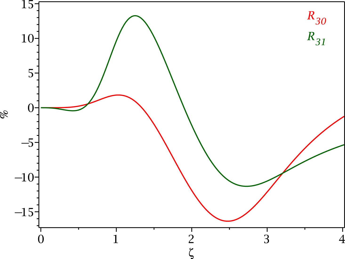
Figure 4. The
 $\%$
error of the imaginary parts of
$\%$
error of the imaginary parts of
 $R_{3,0}(\unicode[STIX]{x1D701})$
(red line), and
$R_{3,0}(\unicode[STIX]{x1D701})$
(red line), and
 $R_{3,1}(\unicode[STIX]{x1D701})$
(green line).
$R_{3,1}(\unicode[STIX]{x1D701})$
(green line).
By exploring the expressions inside of the brackets, it is obvious that it is impossible to express
 $q^{(1)}$
or
$q^{(1)}$
or
 $\widetilde{r}^{(1)}$
as a linear combination of lower-order moments that eliminate the
$\widetilde{r}^{(1)}$
as a linear combination of lower-order moments that eliminate the
 $\unicode[STIX]{x1D701}$
dependence. Moreover, for large
$\unicode[STIX]{x1D701}$
dependence. Moreover, for large
 $\unicode[STIX]{x1D701}$
, the moments
$\unicode[STIX]{x1D701}$
, the moments
 $q^{(1)}\sim \unicode[STIX]{x1D701}^{2}$
and
$q^{(1)}\sim \unicode[STIX]{x1D701}^{2}$
and
 $\widetilde{r}^{(1)}\sim \unicode[STIX]{x1D701}^{3}$
, which does not make physical sense, since these quantities should converge to zero with increasing
$\widetilde{r}^{(1)}\sim \unicode[STIX]{x1D701}^{3}$
, which does not make physical sense, since these quantities should converge to zero with increasing
 $\unicode[STIX]{x1D701}$
, as explored in the
$\unicode[STIX]{x1D701}$
, as explored in the
 $\unicode[STIX]{x1D701}\gg 1$
limit, see equations (3.80)–(3.86). The
$\unicode[STIX]{x1D701}\gg 1$
limit, see equations (3.80)–(3.86). The
 $R_{1}(\unicode[STIX]{x1D701})$
approximant therefore does not yield a closure. The same conclusion is obtained by using the
$R_{1}(\unicode[STIX]{x1D701})$
approximant therefore does not yield a closure. The same conclusion is obtained by using the
 $R_{2,0}(\unicode[STIX]{x1D701})$
approximant, where no closure for
$R_{2,0}(\unicode[STIX]{x1D701})$
approximant, where no closure for
 $q^{(1)}$
or
$q^{(1)}$
or
 $\widetilde{r}^{(1)}$
is possible. We note that the approximant
$\widetilde{r}^{(1)}$
is possible. We note that the approximant
 $R_{2,1}(\unicode[STIX]{x1D701})$
, that was eliminated because it is not a good approximant of
$R_{2,1}(\unicode[STIX]{x1D701})$
, that was eliminated because it is not a good approximant of
 $R(\unicode[STIX]{x1D701})$
yields a closure
$R(\unicode[STIX]{x1D701})$
yields a closure
 $q^{(1)}=-2p_{0}u^{(1)}$
, which is equivalent to the closure (3.49), that was obtained for small
$q^{(1)}=-2p_{0}u^{(1)}$
, which is equivalent to the closure (3.49), that was obtained for small
 $\unicode[STIX]{x1D701}$
with the precision
$\unicode[STIX]{x1D701}$
with the precision
 $o(\unicode[STIX]{x1D701})$
. This closure is therefore disregarded.
$o(\unicode[STIX]{x1D701})$
. This closure is therefore disregarded.
Let us try the three-pole Padé approximants. The moments with
 $R_{3,1}(\unicode[STIX]{x1D701})$
approximant are proportional to
$R_{3,1}(\unicode[STIX]{x1D701})$
approximant are proportional to
 $$\begin{eqnarray}\displaystyle R_{3,1}(\unicode[STIX]{x1D701}):\quad n^{(1)} & {\sim} & \displaystyle \frac{1}{1-{\displaystyle \frac{4i}{\sqrt{\unicode[STIX]{x03C0}}}}\unicode[STIX]{x1D701}-2\unicode[STIX]{x1D701}^{2}+2i{\displaystyle \frac{4-\unicode[STIX]{x03C0}}{\sqrt{\unicode[STIX]{x03C0}}}}\unicode[STIX]{x1D701}^{3}}\left[1+\frac{i}{\sqrt{\unicode[STIX]{x03C0}}}(\unicode[STIX]{x03C0}-4)\unicode[STIX]{x1D701}\right];\end{eqnarray}$$
 $$\begin{eqnarray}\displaystyle u^{(1)} & {\sim} & \displaystyle \frac{1}{1-{\displaystyle \frac{4i}{\sqrt{\unicode[STIX]{x03C0}}}}\unicode[STIX]{x1D701}-2\unicode[STIX]{x1D701}^{2}+2i{\displaystyle \frac{4-\unicode[STIX]{x03C0}}{\sqrt{\unicode[STIX]{x03C0}}}}\unicode[STIX]{x1D701}^{3}}\left[\frac{i}{\sqrt{\unicode[STIX]{x03C0}}}(\unicode[STIX]{x03C0}-4)\unicode[STIX]{x1D701}^{2}+\unicode[STIX]{x1D701}\right];\end{eqnarray}$$
 $$\begin{eqnarray}\displaystyle T^{(1)} & {\sim} & \displaystyle \frac{1}{1-{\displaystyle \frac{4i}{\sqrt{\unicode[STIX]{x03C0}}}}\unicode[STIX]{x1D701}-2\unicode[STIX]{x1D701}^{2}+2i{\displaystyle \frac{4-\unicode[STIX]{x03C0}}{\sqrt{\unicode[STIX]{x03C0}}}}\unicode[STIX]{x1D701}^{3}}\left[-i\sqrt{\unicode[STIX]{x03C0}}\unicode[STIX]{x1D701}\right];\end{eqnarray}$$
 $$\begin{eqnarray}\displaystyle q^{(1)} & {\sim} & \displaystyle \frac{1}{1-{\displaystyle \frac{4i}{\sqrt{\unicode[STIX]{x03C0}}}}\unicode[STIX]{x1D701}-2\unicode[STIX]{x1D701}^{2}+2i{\displaystyle \frac{4-\unicode[STIX]{x03C0}}{\sqrt{\unicode[STIX]{x03C0}}}}\unicode[STIX]{x1D701}^{3}}\left[-\frac{i}{\sqrt{\unicode[STIX]{x03C0}}}(3\unicode[STIX]{x03C0}-8)\unicode[STIX]{x1D701}^{2}-2\unicode[STIX]{x1D701}\right];\end{eqnarray}$$
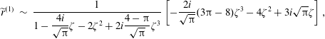 $$\begin{eqnarray}\displaystyle \widetilde{r}^{(1)} & {\sim} & \displaystyle {\displaystyle \frac{1}{1-{\displaystyle \frac{4i}{\sqrt{\unicode[STIX]{x03C0}}}}\unicode[STIX]{x1D701}-2\unicode[STIX]{x1D701}^{2}+2i{\displaystyle \frac{4-\unicode[STIX]{x03C0}}{\sqrt{\unicode[STIX]{x03C0}}}}\unicode[STIX]{x1D701}^{3}}}\left[-\frac{2i}{\sqrt{\unicode[STIX]{x03C0}}}(3\unicode[STIX]{x03C0}-8)\unicode[STIX]{x1D701}^{3}-4\unicode[STIX]{x1D701}^{2}+3i\sqrt{\unicode[STIX]{x03C0}}\unicode[STIX]{x1D701}\right],\nonumber\\ \displaystyle & & \displaystyle\end{eqnarray}$$
where we have suppressed writing all the multiplicative factors including the minus signs (it does not mean that these were neglected, full expressions are considered, we are just not writing down the full expressions, which helps in spotting the possible closures). There is a possibility of expressing
 $q^{(1)}$
through the combination of the lower moments
$q^{(1)}$
through the combination of the lower moments
 $T^{(1)}$
and
$T^{(1)}$
and
 $u^{(1)}$
. The full expressions of these moments are
$u^{(1)}$
. The full expressions of these moments are
 $$\begin{eqnarray}\displaystyle R_{3,1}(\unicode[STIX]{x1D701}):\quad D & = & \displaystyle \left(1-\frac{4i}{\sqrt{\unicode[STIX]{x03C0}}}\unicode[STIX]{x1D701}-2\unicode[STIX]{x1D701}^{2}+2i\frac{4-\unicode[STIX]{x03C0}}{\sqrt{\unicode[STIX]{x03C0}}}\unicode[STIX]{x1D701}^{3}\right);\end{eqnarray}$$
 $$\begin{eqnarray}\displaystyle u^{(1)} & = & \displaystyle -\frac{q_{r}}{T^{(0)}}\unicode[STIX]{x1D6F7}v_{\text{th}}\text{sign}(k_{\Vert })\frac{1}{D}\left[\frac{i}{\sqrt{\unicode[STIX]{x03C0}}}(\unicode[STIX]{x03C0}-4)\unicode[STIX]{x1D701}^{2}+\unicode[STIX]{x1D701}\right];\end{eqnarray}$$
 $$\begin{eqnarray}\displaystyle T^{(1)} & = & \displaystyle -q_{r}\unicode[STIX]{x1D6F7}\frac{1}{D}\left[-i\sqrt{\unicode[STIX]{x03C0}}\unicode[STIX]{x1D701}\right];\end{eqnarray}$$
 $$\begin{eqnarray}\displaystyle q^{(1)} & = & \displaystyle -q_{r}n_{0}\unicode[STIX]{x1D6F7}v_{\text{th}}\text{sign}(k_{\Vert })\frac{1}{D}\left[-\frac{i}{\sqrt{\unicode[STIX]{x03C0}}}(3\unicode[STIX]{x03C0}-8)\unicode[STIX]{x1D701}^{2}-2\unicode[STIX]{x1D701}\right],\end{eqnarray}$$
where we have used a convenient notation
 $D$
for the denominator of the plasma response function, and the closure is
$D$
for the denominator of the plasma response function, and the closure is
which is equivalent to the (3.60) closure (which was obtained for small
 $\unicode[STIX]{x1D701}$
with the precision
$\unicode[STIX]{x1D701}$
with the precision
 $o(\unicode[STIX]{x1D701}^{2})$
). Continuing with the next approximant
$o(\unicode[STIX]{x1D701}^{2})$
). Continuing with the next approximant
 $R_{3,2}(\unicode[STIX]{x1D701})$
, the moments calculate as
$R_{3,2}(\unicode[STIX]{x1D701})$
, the moments calculate as
 $$\begin{eqnarray}\displaystyle R_{3,2}(\unicode[STIX]{x1D701}):\quad D & = & \displaystyle \left(1-\frac{3i\sqrt{\unicode[STIX]{x03C0}}}{2}\unicode[STIX]{x1D701}-2\unicode[STIX]{x1D701}^{2}+i\sqrt{\unicode[STIX]{x03C0}}\unicode[STIX]{x1D701}^{3}\right);\end{eqnarray}$$
 $$\begin{eqnarray}\displaystyle n^{(1)} & {\sim} & \displaystyle \frac{1}{D}\left[1-\frac{i\sqrt{\unicode[STIX]{x03C0}}}{2}\unicode[STIX]{x1D701}\right];\end{eqnarray}$$
 $$\begin{eqnarray}\displaystyle u^{(1)} & {\sim} & \displaystyle \frac{1}{D}\left[-\frac{i\sqrt{\unicode[STIX]{x03C0}}}{2}\unicode[STIX]{x1D701}^{2}+\unicode[STIX]{x1D701}\right];\end{eqnarray}$$
 $$\begin{eqnarray}\displaystyle T^{(1)} & {\sim} & \displaystyle \frac{1}{D}\left[-i\sqrt{\unicode[STIX]{x03C0}}\unicode[STIX]{x1D701}\right];\end{eqnarray}$$
 $$\begin{eqnarray}\displaystyle q^{(1)} & {\sim} & \displaystyle \frac{1}{D}\left[-2\unicode[STIX]{x1D701}\right];\end{eqnarray}$$
 $$\begin{eqnarray}\displaystyle \widetilde{r}^{(1)} & {\sim} & \displaystyle \frac{1}{D}\left[-4\unicode[STIX]{x1D701}^{2}+3i\sqrt{\unicode[STIX]{x03C0}}\unicode[STIX]{x1D701}\right].\end{eqnarray}$$
It is possible to express (1)
 $q^{(1)}$
through
$q^{(1)}$
through
 $T^{(1)}$
; (2)
$T^{(1)}$
; (2)
 $\widetilde{r}^{(1)}$
through the combination of
$\widetilde{r}^{(1)}$
through the combination of
 $u^{(1)}$
and
$u^{(1)}$
and
 $q^{(1)}$
; (3)
$q^{(1)}$
; (3)
 $\widetilde{r}^{(1)}$
through the combination of
$\widetilde{r}^{(1)}$
through the combination of
 $u^{(1)}$
and
$u^{(1)}$
and
 $T^{(1)}$
. The first choice yields a closure
$T^{(1)}$
. The first choice yields a closure
that is equivalent to the (3.48) closure obtained for small
 $\unicode[STIX]{x1D701}$
with the precision
$\unicode[STIX]{x1D701}$
with the precision
 $o(\unicode[STIX]{x1D701})$
. This is indeed the famous simplest possible Landau fluid closure that expresses the collisionless heat flux with respect to temperature, and it equivalent to equation (7) of Hammett & Perkins (Reference Hammett and Perkins1990).Footnote
8
The closure is written here in Fourier space. The important part is the
$o(\unicode[STIX]{x1D701})$
. This is indeed the famous simplest possible Landau fluid closure that expresses the collisionless heat flux with respect to temperature, and it equivalent to equation (7) of Hammett & Perkins (Reference Hammett and Perkins1990).Footnote
8
The closure is written here in Fourier space. The important part is the
 $i\text{sign}(k_{\Vert })$
that typically written as
$i\text{sign}(k_{\Vert })$
that typically written as
 $ik_{\Vert }/|k_{\Vert }|$
, and that in real space rewrites as a Hilbert transform, which we will address later. The
$ik_{\Vert }/|k_{\Vert }|$
, and that in real space rewrites as a Hilbert transform, which we will address later. The
 $R_{3,2}(\unicode[STIX]{x1D701})$
was obtained with
$R_{3,2}(\unicode[STIX]{x1D701})$
was obtained with
 $o(\unicode[STIX]{x1D701})$
power-series expansion, and
$o(\unicode[STIX]{x1D701})$
power-series expansion, and
 $o(1/\unicode[STIX]{x1D701}^{4})$
asymptotic-series expansion. How good is this closure? By exploring expressions (3.212)–(3.216), the quantities
$o(1/\unicode[STIX]{x1D701}^{4})$
asymptotic-series expansion. How good is this closure? By exploring expressions (3.212)–(3.216), the quantities
 $n^{(1)}$
,
$n^{(1)}$
,
 $u^{(1)}$
,
$u^{(1)}$
,
 $T^{(1)}$
have all correct asymptotic expansion for large
$T^{(1)}$
have all correct asymptotic expansion for large
 $\unicode[STIX]{x1D701}$
(including the proportionality constants), however, the heat flux decreases only as
$\unicode[STIX]{x1D701}$
(including the proportionality constants), however, the heat flux decreases only as
 $q^{(1)}\sim 1/\unicode[STIX]{x1D701}^{2}$
instead of the correct
$q^{(1)}\sim 1/\unicode[STIX]{x1D701}^{2}$
instead of the correct
 ${\sim}1/\unicode[STIX]{x1D701}^{3}$
, see (3.84). For large
${\sim}1/\unicode[STIX]{x1D701}^{3}$
, see (3.84). For large
 $\unicode[STIX]{x1D701}$
, the heat flux is therefore overestimated by this simple closure, which typically leads to an overestimation of the Landau damping in fluid models that use this simplest closure. Nevertheless, the closure is very beneficial because it clarifies the distinction between the collisional and collisionless heat fluxes.
$\unicode[STIX]{x1D701}$
, the heat flux is therefore overestimated by this simple closure, which typically leads to an overestimation of the Landau damping in fluid models that use this simplest closure. Nevertheless, the closure is very beneficial because it clarifies the distinction between the collisional and collisionless heat fluxes.
The other two possible closures with
 $R_{3,2}(\unicode[STIX]{x1D701})$
are
$R_{3,2}(\unicode[STIX]{x1D701})$
are
 $$\begin{eqnarray}\displaystyle R_{3,2}(\unicode[STIX]{x1D701}):\quad \widetilde{r}^{(1)} & = & \displaystyle -\frac{4i}{\sqrt{\unicode[STIX]{x03C0}}}v_{\text{th}}n_{0}T^{(0)}\text{sign}(k_{\Vert })u^{(1)}-i\frac{(3\unicode[STIX]{x03C0}+8)}{4\sqrt{\unicode[STIX]{x03C0}}}v_{\text{th}}\text{sign}(k_{\Vert })q^{(1)};\end{eqnarray}$$
 $$\begin{eqnarray}\displaystyle \widetilde{r}^{(1)} & = & \displaystyle -\frac{4i}{\sqrt{\unicode[STIX]{x03C0}}}v_{\text{th}}n_{0}T^{(0)}\text{sign}(k_{\Vert })u^{(1)}-\frac{(3\unicode[STIX]{x03C0}+8)}{2\unicode[STIX]{x03C0}}v_{\text{th}}^{2}n_{0}T^{(1)},\end{eqnarray}$$
and one can go from (3.219) to (3.220) by using (3.218). Obviously, it would be also possible to construct a closure
 $\widetilde{r}^{(1)}=\unicode[STIX]{x1D6FC}_{u}u^{(1)}+\unicode[STIX]{x1D6FC}_{q}q^{(1)}+\unicode[STIX]{x1D6FC}_{T}T^{(1)}$
, where
$\widetilde{r}^{(1)}=\unicode[STIX]{x1D6FC}_{u}u^{(1)}+\unicode[STIX]{x1D6FC}_{q}q^{(1)}+\unicode[STIX]{x1D6FC}_{T}T^{(1)}$
, where
 $\unicode[STIX]{x1D6FC}_{u}=-(4i/\sqrt{\unicode[STIX]{x03C0}})v_{\text{th}}n_{0}T^{(0)}\text{sign}(k_{\Vert })$
, and where
$\unicode[STIX]{x1D6FC}_{u}=-(4i/\sqrt{\unicode[STIX]{x03C0}})v_{\text{th}}n_{0}T^{(0)}\text{sign}(k_{\Vert })$
, and where
 $\unicode[STIX]{x1D6FC}_{q}$
and
$\unicode[STIX]{x1D6FC}_{q}$
and
 $\unicode[STIX]{x1D6FC}_{T}$
are related by satisfying
$\unicode[STIX]{x1D6FC}_{T}$
are related by satisfying
 $2n_{0}v_{\text{th}}\text{sign}(k_{\Vert })\unicode[STIX]{x1D6FC}_{q}+i\sqrt{\unicode[STIX]{x03C0}}\unicode[STIX]{x1D6FC}_{T}=-iv_{\text{th}}^{2}n_{0}((3\unicode[STIX]{x03C0}+8)/2\sqrt{\unicode[STIX]{x03C0}})$
, i.e. one could consider a closure with a free parameter, which we will not consider. Additionally, all constructed closures should be checked with respect to obtained dispersion relations, and closures (3.219), (3.220) will be later disregarded as not well behaved (see the discussion below equations (3.242), (3.382) and (3.399)).
$2n_{0}v_{\text{th}}\text{sign}(k_{\Vert })\unicode[STIX]{x1D6FC}_{q}+i\sqrt{\unicode[STIX]{x03C0}}\unicode[STIX]{x1D6FC}_{T}=-iv_{\text{th}}^{2}n_{0}((3\unicode[STIX]{x03C0}+8)/2\sqrt{\unicode[STIX]{x03C0}})$
, i.e. one could consider a closure with a free parameter, which we will not consider. Additionally, all constructed closures should be checked with respect to obtained dispersion relations, and closures (3.219), (3.220) will be later disregarded as not well behaved (see the discussion below equations (3.242), (3.382) and (3.399)).
For
 $R_{4,2}(\unicode[STIX]{x1D701})$
, the kinetic moments calculate as
$R_{4,2}(\unicode[STIX]{x1D701})$
, the kinetic moments calculate as
 $$\begin{eqnarray}\displaystyle R_{4,2}(\unicode[STIX]{x1D701}):\quad D & = & \displaystyle \left(1-i\sqrt{\unicode[STIX]{x03C0}}\frac{2}{(3\unicode[STIX]{x03C0}-8)}\unicode[STIX]{x1D701}-\frac{(32-9\unicode[STIX]{x03C0})}{(3\unicode[STIX]{x03C0}-8)}\unicode[STIX]{x1D701}^{2}\right.\nonumber\\ \displaystyle & & \displaystyle \left.+\,i\sqrt{\unicode[STIX]{x03C0}}\frac{2(10-3\unicode[STIX]{x03C0})}{(3\unicode[STIX]{x03C0}-8)}\unicode[STIX]{x1D701}^{3}+\frac{2(16-5\unicode[STIX]{x03C0})}{(3\unicode[STIX]{x03C0}-8)}\unicode[STIX]{x1D701}^{4}\right);\end{eqnarray}$$
 $$\begin{eqnarray}\displaystyle n^{(1)} & {\sim} & \displaystyle \frac{1}{D}\left[\frac{(5\unicode[STIX]{x03C0}-16)}{(3\unicode[STIX]{x03C0}-8)}\unicode[STIX]{x1D701}^{2}+i\sqrt{\unicode[STIX]{x03C0}}\frac{(3\unicode[STIX]{x03C0}-10)}{(3\unicode[STIX]{x03C0}-8)}\unicode[STIX]{x1D701}+1\right];\end{eqnarray}$$
 $$\begin{eqnarray}\displaystyle u^{(1)} & {\sim} & \displaystyle \frac{1}{D}\left[\frac{(5\unicode[STIX]{x03C0}-16)}{(3\unicode[STIX]{x03C0}-8)}\unicode[STIX]{x1D701}^{3}+i\sqrt{\unicode[STIX]{x03C0}}\frac{(3\unicode[STIX]{x03C0}-10)}{(3\unicode[STIX]{x03C0}-8)}\unicode[STIX]{x1D701}^{2}+\unicode[STIX]{x1D701}\right];\end{eqnarray}$$
 $$\begin{eqnarray}\displaystyle T^{(1)} & {\sim} & \displaystyle \frac{1}{D}\left[\frac{2(5\unicode[STIX]{x03C0}-16)}{(3\unicode[STIX]{x03C0}-8)}\unicode[STIX]{x1D701}^{2}-i\sqrt{\unicode[STIX]{x03C0}}\unicode[STIX]{x1D701}\right];\end{eqnarray}$$
 $$\begin{eqnarray}\displaystyle q^{(1)} & {\sim} & \displaystyle \frac{1}{D}\left[-i\sqrt{\unicode[STIX]{x03C0}}\frac{(9\unicode[STIX]{x03C0}-28)}{(3\unicode[STIX]{x03C0}-8)}\unicode[STIX]{x1D701}^{2}-2\unicode[STIX]{x1D701}\right];\end{eqnarray}$$
 $$\begin{eqnarray}\displaystyle \widetilde{r}^{(1)} & {\sim} & \displaystyle \frac{1}{D}\left[-i\sqrt{\unicode[STIX]{x03C0}}\frac{2(9\unicode[STIX]{x03C0}-28)}{(3\unicode[STIX]{x03C0}-8)}\unicode[STIX]{x1D701}^{3}-\frac{2(21\unicode[STIX]{x03C0}-64)}{(3\unicode[STIX]{x03C0}-8)}\unicode[STIX]{x1D701}^{2}+3i\sqrt{\unicode[STIX]{x03C0}}\unicode[STIX]{x1D701}\right].\end{eqnarray}$$
The only possibility is to express
 $\widetilde{r}^{(1)}$
through a combination of
$\widetilde{r}^{(1)}$
through a combination of
 $u^{(1)}$
,
$u^{(1)}$
,
 $T^{(1)}$
and
$T^{(1)}$
and
 $q^{(1)}$
, and the solution is
$q^{(1)}$
, and the solution is
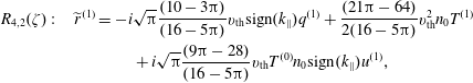 $$\begin{eqnarray}\displaystyle & \displaystyle R_{4,2}(\unicode[STIX]{x1D701}):\quad \widetilde{r}^{(1)}=-i\sqrt{\unicode[STIX]{x03C0}}\frac{(10-3\unicode[STIX]{x03C0})}{(16-5\unicode[STIX]{x03C0})}v_{\text{th}}\text{sign}(k_{\Vert })q^{(1)}+\frac{(21\unicode[STIX]{x03C0}-64)}{2(16-5\unicode[STIX]{x03C0})}v_{\text{th}}^{2}n_{0}T^{(1)} & \displaystyle \nonumber\\ \displaystyle & \displaystyle \qquad \quad +\,i\sqrt{\unicode[STIX]{x03C0}}\frac{(9\unicode[STIX]{x03C0}-28)}{(16-5\unicode[STIX]{x03C0})}v_{\text{th}}T^{(0)}n_{0}\text{sign}(k_{\Vert })u^{(1)}, & \displaystyle\end{eqnarray}$$
which is equivalent to the closure (3.64), that was obtained for small
 $\unicode[STIX]{x1D701}$
with precision
$\unicode[STIX]{x1D701}$
with precision
 $o(\unicode[STIX]{x1D701}^{3})$
. Obviously such a closure is precise for small values of
$o(\unicode[STIX]{x1D701}^{3})$
. Obviously such a closure is precise for small values of
 $\unicode[STIX]{x1D701}$
, however for large values of
$\unicode[STIX]{x1D701}$
, however for large values of
 $\unicode[STIX]{x1D701}$
, the asymptotic behaviour of
$\unicode[STIX]{x1D701}$
, the asymptotic behaviour of
 $q^{(1)}\sim \unicode[STIX]{x1D701}^{-2}$
and
$q^{(1)}\sim \unicode[STIX]{x1D701}^{-2}$
and
 $\widetilde{r}^{(1)}\sim \unicode[STIX]{x1D701}^{-1}$
, instead of the correct
$\widetilde{r}^{(1)}\sim \unicode[STIX]{x1D701}^{-1}$
, instead of the correct
 $\unicode[STIX]{x1D701}^{-3},\unicode[STIX]{x1D701}^{-4}$
profiles (see (3.84), (3.86)), and these quantities will be therefore overestimated. Nevertheless, the solution is interesting and we are not aware of it being reporting in any literature.
$\unicode[STIX]{x1D701}^{-3},\unicode[STIX]{x1D701}^{-4}$
profiles (see (3.84), (3.86)), and these quantities will be therefore overestimated. Nevertheless, the solution is interesting and we are not aware of it being reporting in any literature.
Continuing with
 $R_{4,3}(\unicode[STIX]{x1D701})$
, the kinetic moments calculate as
$R_{4,3}(\unicode[STIX]{x1D701})$
, the kinetic moments calculate as
 $$\begin{eqnarray}\displaystyle R_{4,3}(\unicode[STIX]{x1D701}):\quad D & = & \displaystyle \left(1-i\frac{3\sqrt{\unicode[STIX]{x03C0}}}{2}\unicode[STIX]{x1D701}-\frac{(9\unicode[STIX]{x03C0}-16)}{4}\unicode[STIX]{x1D701}^{2}+i\sqrt{\unicode[STIX]{x03C0}}\unicode[STIX]{x1D701}^{3}+\frac{(3\unicode[STIX]{x03C0}-8)}{2}\unicode[STIX]{x1D701}^{4}\right);\nonumber\\ \displaystyle & & \displaystyle\end{eqnarray}$$
 $$\begin{eqnarray}\displaystyle n^{(1)} & {\sim} & \displaystyle \frac{1}{D}\left[\frac{(8-3\unicode[STIX]{x03C0})}{4}\unicode[STIX]{x1D701}^{2}-i\frac{\sqrt{\unicode[STIX]{x03C0}}}{2}\unicode[STIX]{x1D701}+1\right];\end{eqnarray}$$
 $$\begin{eqnarray}\displaystyle u^{(1)} & {\sim} & \displaystyle \frac{1}{D}\left[\frac{(8-3\unicode[STIX]{x03C0})}{4}\unicode[STIX]{x1D701}^{3}-i\frac{\sqrt{\unicode[STIX]{x03C0}}}{2}\unicode[STIX]{x1D701}^{2}+\unicode[STIX]{x1D701}\right];\end{eqnarray}$$
 $$\begin{eqnarray}\displaystyle T^{(1)} & {\sim} & \displaystyle \frac{1}{D}\left[\frac{(8-3\unicode[STIX]{x03C0})}{2}\unicode[STIX]{x1D701}^{2}-i\sqrt{\unicode[STIX]{x03C0}}\unicode[STIX]{x1D701}\right];\end{eqnarray}$$
 $$\begin{eqnarray}\displaystyle q^{(1)} & {\sim} & \displaystyle \frac{1}{D}\left[-2\unicode[STIX]{x1D701}\right];\end{eqnarray}$$
 $$\begin{eqnarray}\displaystyle \widetilde{r}^{(1)} & {\sim} & \displaystyle \frac{1}{D}\left[\frac{(9\unicode[STIX]{x03C0}-32)}{2}\unicode[STIX]{x1D701}^{2}+3i\sqrt{\unicode[STIX]{x03C0}}\unicode[STIX]{x1D701}\right].\end{eqnarray}$$
It is possible to express
 $\widetilde{r}^{(1)}$
through the combination of
$\widetilde{r}^{(1)}$
through the combination of
 $q^{(1)}$
and
$q^{(1)}$
and
 $T^{(1)}$
and the result is
$T^{(1)}$
and the result is
which is equivalent to the closure (3.56), that was obtained for small
 $\unicode[STIX]{x1D701}$
with the precision
$\unicode[STIX]{x1D701}$
with the precision
 $o(\unicode[STIX]{x1D701}^{2})$
. The heat flux has a correct asymptotic behaviour
$o(\unicode[STIX]{x1D701}^{2})$
. The heat flux has a correct asymptotic behaviour
 $q^{(1)}\sim \unicode[STIX]{x1D701}^{-3}$
(even though with incorrect proportionality constant), and the quantity
$q^{(1)}\sim \unicode[STIX]{x1D701}^{-3}$
(even though with incorrect proportionality constant), and the quantity
 $\widetilde{r}^{(1)}\sim \unicode[STIX]{x1D701}^{-2}$
instead of the correct
$\widetilde{r}^{(1)}\sim \unicode[STIX]{x1D701}^{-2}$
instead of the correct
 ${\sim}\unicode[STIX]{x1D701}^{-4}$
. The closure was first reported by Hammett & Perkins (Reference Hammett and Perkins1990), and is equivalent to the (non-numbered) expression between their equations (10) and (11).
${\sim}\unicode[STIX]{x1D701}^{-4}$
. The closure was first reported by Hammett & Perkins (Reference Hammett and Perkins1990), and is equivalent to the (non-numbered) expression between their equations (10) and (11).
Continuing with
 $R_{4,4}(\unicode[STIX]{x1D701})$
approximant, the kinetic moments are (let us stop writing down
$R_{4,4}(\unicode[STIX]{x1D701})$
approximant, the kinetic moments are (let us stop writing down
 $n^{(1)}$
from now on since we know we can get it from
$n^{(1)}$
from now on since we know we can get it from
 $u^{(1)}$
)
$u^{(1)}$
)
 $$\begin{eqnarray}\displaystyle R_{4,4}(\unicode[STIX]{x1D701}):\quad D & = & \displaystyle \left(1-i\frac{3\sqrt{\unicode[STIX]{x03C0}}}{2}\unicode[STIX]{x1D701}-4\unicode[STIX]{x1D701}^{2}+i\sqrt{\unicode[STIX]{x03C0}}\unicode[STIX]{x1D701}^{3}+\frac{4}{3}\unicode[STIX]{x1D701}^{4}\right);\end{eqnarray}$$
 $$\begin{eqnarray}\displaystyle u^{(1)} & {\sim} & \displaystyle \frac{1}{D}\left[-\frac{2}{3}\unicode[STIX]{x1D701}^{3}-\frac{i}{2}\sqrt{\unicode[STIX]{x03C0}}\unicode[STIX]{x1D701}^{2}+\unicode[STIX]{x1D701}\right];\end{eqnarray}$$
 $$\begin{eqnarray}\displaystyle T^{(1)} & {\sim} & \displaystyle \frac{1}{D}\left[-\frac{4}{3}\unicode[STIX]{x1D701}^{2}-i\sqrt{\unicode[STIX]{x03C0}}\unicode[STIX]{x1D701}\right];\end{eqnarray}$$
 $$\begin{eqnarray}\displaystyle q^{(1)} & {\sim} & \displaystyle \frac{1}{D}\left[-2\unicode[STIX]{x1D701}\right];\end{eqnarray}$$
 $$\begin{eqnarray}\displaystyle \widetilde{r}^{(1)} & {\sim} & \displaystyle \frac{1}{D}\left[3i\sqrt{\unicode[STIX]{x03C0}}\unicode[STIX]{x1D701}\right].\end{eqnarray}$$
It is possible to express
 $\widetilde{r}^{(1)}$
through
$\widetilde{r}^{(1)}$
through
 $q^{(1)}$
and the closure is
$q^{(1)}$
and the closure is
The result is equivalent to the (3.52) closure, that was obtained for small
 $\unicode[STIX]{x1D701}$
with precision
$\unicode[STIX]{x1D701}$
with precision
 $o(\unicode[STIX]{x1D701})$
. This very simple closure has only precision
$o(\unicode[STIX]{x1D701})$
. This very simple closure has only precision
 $o(\unicode[STIX]{x1D701})$
, however, it does have the correct asymptotic behaviour of the heat flux
$o(\unicode[STIX]{x1D701})$
, however, it does have the correct asymptotic behaviour of the heat flux
 $q^{(1)}\sim -3/(2\unicode[STIX]{x1D701}^{3})$
(including the proportionality constant), and
$q^{(1)}\sim -3/(2\unicode[STIX]{x1D701}^{3})$
(including the proportionality constant), and
 $\widetilde{r}^{(1)}\sim \unicode[STIX]{x1D701}^{-3}$
that is closer to the correct
$\widetilde{r}^{(1)}\sim \unicode[STIX]{x1D701}^{-3}$
that is closer to the correct
 $\unicode[STIX]{x1D701}^{-4}$
than the previous closure.
$\unicode[STIX]{x1D701}^{-4}$
than the previous closure.
3.7 Table of moments
$(u_{\Vert },T_{\Vert },q_{\Vert },\widetilde{r}_{\Vert \Vert })$
for various Padé approximants

To clearly see possibilities of a closure, it is useful to create the following summarizing table, that is self-explanatory after reading the previous section, i.e. all the proportionality constants (including the minus signs) are suppressed. Even though the table here is created for a 1-D geometry, we will see that exactly the same table is constructed for a 3-D geometry, where all the quantities are given a ‘parallel’ sub-index, i.e.
 $u^{(1)}\rightarrow u_{\Vert }^{(1)}$
,
$u^{(1)}\rightarrow u_{\Vert }^{(1)}$
,
 $T^{(1)}\rightarrow T_{\Vert }^{(1)}$
,
$T^{(1)}\rightarrow T_{\Vert }^{(1)}$
,
 $q^{(1)}\rightarrow q_{\Vert }^{(1)}$
and
$q^{(1)}\rightarrow q_{\Vert }^{(1)}$
and
 $\widetilde{r}^{(1)}\rightarrow \widetilde{r}_{\Vert \Vert }^{(1)}$
. The table is therefore useful to spot all the possible closures that can be constructed in a 1-D geometry for quantities
$\widetilde{r}^{(1)}\rightarrow \widetilde{r}_{\Vert \Vert }^{(1)}$
. The table is therefore useful to spot all the possible closures that can be constructed in a 1-D geometry for quantities
 $q^{(1)},\widetilde{r}^{(1)}$
, as well as in a 3-D geometry for quantities
$q^{(1)},\widetilde{r}^{(1)}$
, as well as in a 3-D geometry for quantities
 $q_{\Vert }^{(1)}$
and
$q_{\Vert }^{(1)}$
and
 $r_{\Vert \Vert }^{(1)}$
. The approximants
$r_{\Vert \Vert }^{(1)}$
. The approximants
 $R_{2,1},R_{4,5},R_{6,9}$
and
$R_{2,1},R_{4,5},R_{6,9}$
and
 $R_{8,13}$
are marked with an asterisk ‘*’. These approximants are not well behaved (because the Landau residue is not accounted for) and are provided only for completeness, these approximants should be disregarded.
$R_{8,13}$
are marked with an asterisk ‘*’. These approximants are not well behaved (because the Landau residue is not accounted for) and are provided only for completeness, these approximants should be disregarded.
It is obvious by now that any higher-order Padé approximants will not help to achieve a closure. Or is it? One might still hope for ‘a miracle’ thinking that perhaps the seven-pole and eight-pole approximants with the maximum possible number of poles devoted to the asymptotic series –
 $R_{7,10}$
and
$R_{7,10}$
and
 $R_{8,12}$
– might yield a closure. However, this is unfortunately not the case, and the table for seven-pole and eight-pole approximants reads
$R_{8,12}$
– might yield a closure. However, this is unfortunately not the case, and the table for seven-pole and eight-pole approximants reads

By observing the entire table, there are 7 possible quasi-static closures (that were already addressed),
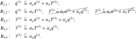
There are also 13 time-dependent closures (that are addressed in the next section),
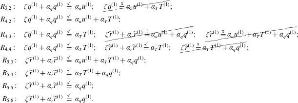
New closures should be always checked. Later on, we will consider propagation of the ion-acoustic mode, satisfying kinetic dispersion relation (3.366). We believe that a good ‘reliable’ closure of a fluid model obtained with the
 $R_{n,n^{\prime }}(\unicode[STIX]{x1D701})$
approximant, should yield a fluid dispersion relation that is equivalent to (3.366), after
$R_{n,n^{\prime }}(\unicode[STIX]{x1D701})$
approximant, should yield a fluid dispersion relation that is equivalent to (3.366), after
 $R(\unicode[STIX]{x1D701})$
is replaced with
$R(\unicode[STIX]{x1D701})$
is replaced with
 $R_{n,n^{\prime }}(\unicode[STIX]{x1D701})$
(equivalent to the numerator of (3.366) once both terms are written with the common denominator). Closures that satisfy this requirement are marked with ‘
$R_{n,n^{\prime }}(\unicode[STIX]{x1D701})$
(equivalent to the numerator of (3.366) once both terms are written with the common denominator). Closures that satisfy this requirement are marked with ‘
 ${\checkmark}$
’ in the above table. Closures that do not satisfy this requirement were eliminated, and can be further split to two categories. Both eliminated categories actually appear to describe the ion-acoustic mode with the same accuracy as a corresponding ‘reliable’ closure satisfying (3.366), however, the difference is in the higher-order modes. The first category of eliminated closures, marked with ‘x’, produces higher-order modes with positive growth rate, and these closures cannot be used for numerical simulations. The second category, marked with ‘!’, produces higher-order modes that are damped, and these closures can still be useful. However, there is no guarantee that these closures will behave well in different circumstances (for example when used in a 3-D geometry) and these closures were therefore eliminated.
${\checkmark}$
’ in the above table. Closures that do not satisfy this requirement were eliminated, and can be further split to two categories. Both eliminated categories actually appear to describe the ion-acoustic mode with the same accuracy as a corresponding ‘reliable’ closure satisfying (3.366), however, the difference is in the higher-order modes. The first category of eliminated closures, marked with ‘x’, produces higher-order modes with positive growth rate, and these closures cannot be used for numerical simulations. The second category, marked with ‘!’, produces higher-order modes that are damped, and these closures can still be useful. However, there is no guarantee that these closures will behave well in different circumstances (for example when used in a 3-D geometry) and these closures were therefore eliminated.
3.8 Going back from Fourier space to real space – the Hilbert transform
The quasi-static Landau fluid closures explored in the previous section were constructed in Fourier space. For direct numerical simulations that can use Fourier transforms (that are usually restricted to periodic boundaries), or for solving dispersion relations
 $\unicode[STIX]{x1D714}(\boldsymbol{k})$
, this is the easiest and natural way how to implement these closures. Nevertheless, it is very beneficial to see how these advanced fluid closures translate to real space.
$\unicode[STIX]{x1D714}(\boldsymbol{k})$
, this is the easiest and natural way how to implement these closures. Nevertheless, it is very beneficial to see how these advanced fluid closures translate to real space.
Provided all equations are linear (and homogeneous), transformation between real and Fourier space is usually very easy and so far we just needed
 $$\begin{eqnarray}\frac{\unicode[STIX]{x2202}}{\unicode[STIX]{x2202}t}\rightarrow -i\unicode[STIX]{x1D714};\quad \unicode[STIX]{x1D735}\rightarrow i\boldsymbol{k};\quad f(\boldsymbol{x},t)\rightarrow \hat{f}(\boldsymbol{k},\unicode[STIX]{x1D714}),\end{eqnarray}$$
where we did not even bother to write the hat symbol on the quantities in Fourier space, since it was obvious and not necessary.
With equations encountered in simple fluid models, transformation back to real space is easy and one can usually just flip the direction of the arrow in relations (3.243). However, the constructed Landau fluid closures contain an unusual operator
 $i\text{sign}(k_{\Vert })=ik_{\Vert }/|k_{\Vert }|$
. How does this operator transforms to real space? Considering spatial 1-D transformation between coordinates
$i\text{sign}(k_{\Vert })=ik_{\Vert }/|k_{\Vert }|$
. How does this operator transforms to real space? Considering spatial 1-D transformation between coordinates
 $z\leftrightarrow k_{\Vert }$
, a general function Fourier transforms according to
$z\leftrightarrow k_{\Vert }$
, a general function Fourier transforms according to
 $$\begin{eqnarray}\displaystyle & \displaystyle f(z)=\frac{1}{2\unicode[STIX]{x03C0}}\int _{-\infty }^{\infty }\hat{f}(k_{\Vert })e^{ik_{\Vert }z}\,\text{d}k_{\Vert }\equiv {\mathcal{F}}^{-1}\hat{f}(k_{\Vert }); & \displaystyle\end{eqnarray}$$
 $$\begin{eqnarray}\displaystyle & \displaystyle \hat{f}(k_{\Vert })=\int _{-\infty }^{\infty }f(z)e^{-ik_{\Vert }z}\,\text{d}z\equiv {\mathcal{F}}f(z), & \displaystyle\end{eqnarray}$$
where the first equation is the inverse/backward Fourier transform and the second equation is the forward Fourier transform. As usual, we often do not bother to write the hat symbols on quantities in Fourier space. The location of the normalization factor
 $1/(2\unicode[STIX]{x03C0})$
is an ad hoc choice, but one has to be consistent, especially when calculating convolutions. As a first step, we need to calculate
$1/(2\unicode[STIX]{x03C0})$
is an ad hoc choice, but one has to be consistent, especially when calculating convolutions. As a first step, we need to calculate
 ${\mathcal{F}}^{-1}$
of a function
${\mathcal{F}}^{-1}$
of a function
 $\text{sign}(k_{\Vert })$
. However, if such an integral is calculated directly, one will find out that the result is not clearly defined.
$\text{sign}(k_{\Vert })$
. However, if such an integral is calculated directly, one will find out that the result is not clearly defined.
It is beneficial to use a small trick, where instead of a function
 $\text{sign}(k_{\Vert })$
, one considers the function
$\text{sign}(k_{\Vert })$
, one considers the function
 $\text{sign}(k_{\Vert })e^{-\unicode[STIX]{x1D6FC}|k_{\Vert }|}$
, where
$\text{sign}(k_{\Vert })e^{-\unicode[STIX]{x1D6FC}|k_{\Vert }|}$
, where
 $\unicode[STIX]{x1D6FC}$
is some small positive constant
$\unicode[STIX]{x1D6FC}$
is some small positive constant
 $\unicode[STIX]{x1D6FC}>0$
. And after the calculation, one performs the limit
$\unicode[STIX]{x1D6FC}>0$
. And after the calculation, one performs the limit
 $\unicode[STIX]{x1D6FC}\rightarrow 0$
. The considered function is
$\unicode[STIX]{x1D6FC}\rightarrow 0$
. The considered function is
 $$\begin{eqnarray}\text{sign}(k_{\Vert })e^{-\unicode[STIX]{x1D6FC}|k_{\Vert }|}=\left\{\begin{array}{@{}ll@{}}-e^{+\unicode[STIX]{x1D6FC}k_{\Vert }};\quad & k_{\Vert }<0;\\ +e^{-\unicode[STIX]{x1D6FC}k_{\Vert }};\quad & k_{\Vert }>0,\end{array}\right.\end{eqnarray}$$
and the integral calculates as
 $$\begin{eqnarray}\displaystyle \int _{-\infty }^{\infty }\text{sign}(k_{\Vert })e^{-\unicode[STIX]{x1D6FC}|k_{\Vert }|}e^{ik_{\Vert }z}\,\text{d}k_{\Vert } & = & \displaystyle \int _{-\infty }^{0}(-1)e^{+\unicode[STIX]{x1D6FC}k_{\Vert }}e^{ik_{\Vert }z}\,\text{d}k_{\Vert }+\int _{0}^{\infty }(+1)e^{-\unicode[STIX]{x1D6FC}k_{\Vert }}e^{ik_{\Vert }z}\,\text{d}k_{\Vert }\nonumber\\ \displaystyle & = & \displaystyle -\int _{-\infty }^{0}e^{(+\unicode[STIX]{x1D6FC}+iz)k_{\Vert }}\,\text{d}k_{\Vert }+\int _{0}^{\infty }e^{(-\unicode[STIX]{x1D6FC}+iz)k_{\Vert }}\,\text{d}k_{\Vert }\nonumber\\ \displaystyle & = & \displaystyle \left.-\frac{1}{(\unicode[STIX]{x1D6FC}+iz)}e^{(+\unicode[STIX]{x1D6FC}+iz)k_{\Vert }}\right|_{k_{\Vert }=-\infty }^{0}+\left.\frac{1}{(-\unicode[STIX]{x1D6FC}+iz)}e^{(-\unicode[STIX]{x1D6FC}+iz)k_{\Vert }}\right|_{k_{\Vert }=0}^{\infty }\nonumber\\ \displaystyle & = & \displaystyle -\frac{1}{(\unicode[STIX]{x1D6FC}+iz)}-\frac{1}{(-\unicode[STIX]{x1D6FC}+iz)}\nonumber\\ \displaystyle & = & \displaystyle \frac{-(\unicode[STIX]{x1D6FC}-iz)+(\unicode[STIX]{x1D6FC}+iz)}{(\unicode[STIX]{x1D6FC}+iz)(\unicode[STIX]{x1D6FC}-iz)}=\frac{2iz}{\unicode[STIX]{x1D6FC}^{2}+z^{2}},\end{eqnarray}$$
further yielding
 $$\begin{eqnarray}{\mathcal{F}}^{-1}\left[i\,\text{sign}(k_{\Vert })e^{-\unicode[STIX]{x1D6FC}|k_{\Vert }|}\right]=\frac{1}{2\unicode[STIX]{x03C0}}\int _{-\infty }^{\infty }i\,\text{sign}(k_{\Vert })e^{-\unicode[STIX]{x1D6FC}|k_{\Vert }|}e^{ik_{\Vert }z}\,\text{d}k_{\Vert }=-\frac{z}{\unicode[STIX]{x03C0}(\unicode[STIX]{x1D6FC}^{2}+z^{2})}.\end{eqnarray}$$
By taking the limit
 $\unicode[STIX]{x1D6FC}\rightarrow 0$
,
$\unicode[STIX]{x1D6FC}\rightarrow 0$
,
 $$\begin{eqnarray}\displaystyle {\mathcal{F}}^{-1}\left[i\,\text{sign}(k_{\Vert })\right]=\frac{1}{2\unicode[STIX]{x03C0}}\int _{-\infty }^{\infty }i\,\text{sign}(k_{\Vert })e^{ik_{\Vert }z}\,\text{d}k_{\Vert }=-\frac{1}{\unicode[STIX]{x03C0}z}. & & \displaystyle\end{eqnarray}$$
In Landau fluid closures, the operator
 $i\text{sign}(k_{\Vert })$
acts on a variable
$i\text{sign}(k_{\Vert })$
acts on a variable
 $\hat{f}(k_{\Vert })$
, and to transform this to real space, we need to use a convolution theorem for Fourier transforms. To make sure that we get the normalization factors right, let us calculate it in detail. The convolution between two real functions is defined as
$\hat{f}(k_{\Vert })$
, and to transform this to real space, we need to use a convolution theorem for Fourier transforms. To make sure that we get the normalization factors right, let us calculate it in detail. The convolution between two real functions is defined as
 $$\begin{eqnarray}f(z)\ast g(z)\equiv \int _{-\infty }^{\infty }f(z-z^{\prime })g(z^{\prime })\,\text{d}z^{\prime }.\end{eqnarray}$$
For brevity, let us temporarily suppress the parallel subscript on
 $k_{\Vert }$
and use only
$k_{\Vert }$
and use only
 $k$
. By decomposing the function
$k$
. By decomposing the function
 $f(z-z^{\prime })$
to waves (using the inverse Fourier transform),
$f(z-z^{\prime })$
to waves (using the inverse Fourier transform),
 $f(z-z^{\prime })=(1/2\unicode[STIX]{x03C0})\int _{-\infty }^{\infty }\hat{f}(k_{\Vert })e^{ik(z-z^{\prime })}\,\text{d}k$
, splitting the
$f(z-z^{\prime })=(1/2\unicode[STIX]{x03C0})\int _{-\infty }^{\infty }\hat{f}(k_{\Vert })e^{ik(z-z^{\prime })}\,\text{d}k$
, splitting the
 $e^{ik(z-z^{\prime })}=e^{ikz}e^{-ikz^{\prime }}$
and changing the order of integrals
$e^{ik(z-z^{\prime })}=e^{ikz}e^{-ikz^{\prime }}$
and changing the order of integrals
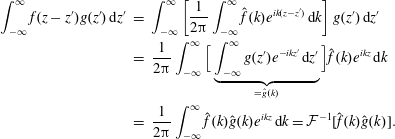 $$\begin{eqnarray}\displaystyle \int _{-\infty }^{\infty }f(z-z^{\prime })g(z^{\prime })\,\text{d}z^{\prime } & = & \displaystyle \int _{-\infty }^{\infty }\left[\frac{1}{2\unicode[STIX]{x03C0}}\int _{-\infty }^{\infty }\hat{f}(k)e^{ik(z-z^{\prime })}\,\text{d}k\right]g(z^{\prime })\,\text{d}z^{\prime }\nonumber\\ \displaystyle & = & \displaystyle \frac{1}{2\unicode[STIX]{x03C0}}\int _{-\infty }^{\infty }\Big[\underbrace{\int _{-\infty }^{\infty }g(z^{\prime })e^{-ikz^{\prime }}\,\text{d}z^{\prime }}_{={\hat{g}}(k)}\Big]\hat{f}(k)e^{ikz}\,\text{d}k\nonumber\\ \displaystyle & = & \displaystyle \frac{1}{2\unicode[STIX]{x03C0}}\int _{-\infty }^{\infty }\hat{f}(k){\hat{g}}(k)e^{ikz}\,\text{d}k={\mathcal{F}}^{-1}[\hat{f}(k){\hat{g}}(k)].\end{eqnarray}$$
For normalizations (3.244), (3.245), the required convolution theorem therefore reads
 $$\begin{eqnarray}{\mathcal{F}}^{-1}[\hat{f}(k_{\Vert }){\hat{g}}(k_{\Vert })]=[{\mathcal{F}}^{-1}\hat{f}(k_{\Vert })]\ast [{\mathcal{F}}^{-1}{\hat{g}}(k_{\Vert })]=f(z)\ast g(z),\end{eqnarray}$$
and of course,
 $f(z)\ast g(z)=g(z)\ast f(z)$
. Now it is straightforward to calculate how
$f(z)\ast g(z)=g(z)\ast f(z)$
. Now it is straightforward to calculate how
 $i\text{sign}(k_{\Vert })\hat{f}(k_{\Vert })$
transforms to real space
$i\text{sign}(k_{\Vert })\hat{f}(k_{\Vert })$
transforms to real space
 $$\begin{eqnarray}\displaystyle {\mathcal{F}}^{-1}[i\text{sign}(k_{\Vert })\hat{f}(k_{\Vert })]=[{\mathcal{F}}^{-1}i\text{sign}(k_{\Vert })]\ast [{\mathcal{F}}^{-1}\hat{f}(k_{\Vert })]=-\frac{1}{\unicode[STIX]{x03C0}z}\ast f(z). & & \displaystyle\end{eqnarray}$$
The convolution of
 $1/\unicode[STIX]{x03C0}z$
with a function
$1/\unicode[STIX]{x03C0}z$
with a function
 $f(z)$
is a famous transformation, called the Hilbert transform. According to the definition (3.250), the convolution
$f(z)$
is a famous transformation, called the Hilbert transform. According to the definition (3.250), the convolution
 $(1/z)\ast f(z)$
should be defined as
$(1/z)\ast f(z)$
should be defined as
 $\int _{-\infty }^{\infty }f(z^{\prime })/(z-z^{\prime })\,\text{d}z^{\prime }$
. However, because of the singularity
$\int _{-\infty }^{\infty }f(z^{\prime })/(z-z^{\prime })\,\text{d}z^{\prime }$
. However, because of the singularity
 $1/(z-z^{\prime })$
, such an integral will likely not exist, and the convolution integral is defined with a principal value. The definition of the Hilbert transform ‘
$1/(z-z^{\prime })$
, such an integral will likely not exist, and the convolution integral is defined with a principal value. The definition of the Hilbert transform ‘
 $H$
’ that is acting on a function
$H$
’ that is acting on a function
 $f(z)$
reads
$f(z)$
reads
 $$\begin{eqnarray}Hf(z)\equiv \frac{1}{\unicode[STIX]{x03C0}z}\ast f(z)\equiv \frac{1}{\unicode[STIX]{x03C0}}V.P.\int _{-\infty }^{\infty }\frac{f(z^{\prime })}{z-z^{\prime }}\,\text{d}z^{\prime }.\end{eqnarray}$$
The use of the Hilbert transform allows a very elegant notation for how the
 $i\text{sign}(k_{\Vert })\hat{f}(k_{\Vert })$
transforms to real space, it is
$i\text{sign}(k_{\Vert })\hat{f}(k_{\Vert })$
transforms to real space, it is
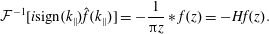 $$\begin{eqnarray}{\mathcal{F}}^{-1}[i\text{sign}(k_{\Vert })\hat{f}(k_{\Vert })]=-\frac{1}{\unicode[STIX]{x03C0}z}\ast f(z)=-Hf(z).\end{eqnarray}$$
Performing a lot of calculations, we like shortcuts, and the quantity
 $i\text{sign}(k_{\Vert })$
can be viewed as an operator, that is acting on many possible
$i\text{sign}(k_{\Vert })$
can be viewed as an operator, that is acting on many possible
 $\hat{f}(k_{\Vert })$
variables, such as the velocity
$\hat{f}(k_{\Vert })$
variables, such as the velocity
 $u^{(1)}$
, the heat flux
$u^{(1)}$
, the heat flux
 $q^{(1)}$
, etc. (see the Landau fluid closures). Therefore, in addition to the usual shortcuts (3.243), we can write an elegant shortcut for the operator
$q^{(1)}$
, etc. (see the Landau fluid closures). Therefore, in addition to the usual shortcuts (3.243), we can write an elegant shortcut for the operator
 $i\text{sign}(k_{\Vert })$
, that is very useful for advanced fluid models when transforming from Fourier to real space, and that reads
$i\text{sign}(k_{\Vert })$
, that is very useful for advanced fluid models when transforming from Fourier to real space, and that reads
Thus, the operator
 $i\text{sign}(k_{\Vert })$
in Fourier space, is the negative Hilbert transform operator in real space. Curiously, does the Hilbert transform integral
$i\text{sign}(k_{\Vert })$
in Fourier space, is the negative Hilbert transform operator in real space. Curiously, does the Hilbert transform integral
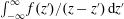 $\int _{-\infty }^{\infty }f(z^{\prime })/(z-z^{\prime })\,\text{d}z^{\prime }$
remind us of something? What about if we prescribe the quantity
$\int _{-\infty }^{\infty }f(z^{\prime })/(z-z^{\prime })\,\text{d}z^{\prime }$
remind us of something? What about if we prescribe the quantity
 $f(z^{\prime })$
to be a Maxwellian
$f(z^{\prime })$
to be a Maxwellian
 $f(z^{\prime })=e^{-z^{\prime 2}}$
? Oh yes, this is the dreadful Landau integral! This is how the plasma dispersion function was essentially defined. This is indeed the reason, why the paper by Fried & Conte (Reference Fried and Conte1961), that is well known for tabulating the properties of the plasma dispersion function, has a full title: ‘The Plasma Dispersion Function. The Hilbert Transform of the Gaussian’.
$f(z^{\prime })=e^{-z^{\prime 2}}$
? Oh yes, this is the dreadful Landau integral! This is how the plasma dispersion function was essentially defined. This is indeed the reason, why the paper by Fried & Conte (Reference Fried and Conte1961), that is well known for tabulating the properties of the plasma dispersion function, has a full title: ‘The Plasma Dispersion Function. The Hilbert Transform of the Gaussian’.
Now we are ready to reformulate the Landau fluid closures in real space. Purely for convenience, often in modern Landau fluid papers another operator
 ${\mathcal{H}}$
is defined that is equivalent to the negative Hilbert transform, and that absorbs the minus sign, i.e.
${\mathcal{H}}$
is defined that is equivalent to the negative Hilbert transform, and that absorbs the minus sign, i.e.
This ‘
 ${\mathcal{H}}$
’ operator is therefore defined as
${\mathcal{H}}$
’ operator is therefore defined as
 $$\begin{eqnarray}\displaystyle {\mathcal{H}}f(z)\equiv -\frac{1}{\unicode[STIX]{x03C0}z}\ast f(z) & \equiv & \displaystyle -\frac{1}{\unicode[STIX]{x03C0}}V.P.\int _{-\infty }^{\infty }\frac{f(z^{\prime })}{z-z^{\prime }}\,\text{d}z^{\prime }=\frac{1}{\unicode[STIX]{x03C0}}V.P.\int _{-\infty }^{\infty }\frac{f(z^{\prime })}{z^{\prime }-z}\,\text{d}z^{\prime }\nonumber\\ \displaystyle & = & \displaystyle -\frac{1}{\unicode[STIX]{x03C0}}V.P.\int _{-\infty }^{\infty }\frac{f(z-z^{\prime })}{z^{\prime }}\,\text{d}z^{\prime },\end{eqnarray}$$
and allows us to write
 $$\begin{eqnarray}{\mathcal{F}}^{-1}[i\text{sign}(k_{\Vert })\hat{f}(k_{\Vert })]={\mathcal{H}}f(z),\end{eqnarray}$$
or in the operator shortcut
This new definition is of course not necessary. However, it is often used in Landau fluid papers, and there is indeed some logic behind it. First of all, we do not have to remember another minus sign, and we will make less typos, perhaps. Second, the definition is consistent with another ‘spatial’ operator Fourier shortcut
 $ik_{\Vert }\rightarrow \unicode[STIX]{x2202}_{z}$
. Third, the Landau integral and the plasma dispersion function were defined with integrals
$ik_{\Vert }\rightarrow \unicode[STIX]{x2202}_{z}$
. Third, the Landau integral and the plasma dispersion function were defined with integrals
 $\int f(x)/(x-x_{0})\,\text{d}x$
, and not as
$\int f(x)/(x-x_{0})\,\text{d}x$
, and not as
 $\int f(x)/(x_{0}-x)\,\text{d}x$
, and the
$\int f(x)/(x_{0}-x)\,\text{d}x$
, and the
 ${\mathcal{H}}$
operator therefore can feel more natural than
${\mathcal{H}}$
operator therefore can feel more natural than
 $H$
. Whatever the choice, we now talked about it in detail, and all possible confusion between
$H$
. Whatever the choice, we now talked about it in detail, and all possible confusion between
 $H$
and
$H$
and
 ${\mathcal{H}}$
should be clarified. We will use the
${\mathcal{H}}$
should be clarified. We will use the
 ${\mathcal{H}}$
operator henceforth.
${\mathcal{H}}$
operator henceforth.
3.9 Quasi-static closures in real space
With our new shortcut (3.260) as discussed above, the transformation of closures from Fourier space to real space is very easy. For example, the heat flux closure obtained for
 $R_{3,2}(\unicode[STIX]{x1D701})$
that in Fourier space reads
$R_{3,2}(\unicode[STIX]{x1D701})$
that in Fourier space reads
 $q^{(1)}=-i(2/\sqrt{\unicode[STIX]{x03C0}})n_{0}v_{\text{th}}\text{sign}(k_{\Vert })T^{(1)}$
, is transferred to real space as
$q^{(1)}=-i(2/\sqrt{\unicode[STIX]{x03C0}})n_{0}v_{\text{th}}\text{sign}(k_{\Vert })T^{(1)}$
, is transferred to real space as
Again, the
 ${\mathcal{H}}$
operator shows its slight advantage over
${\mathcal{H}}$
operator shows its slight advantage over
 $H$
operator, because it is easy to remember that for the usual collisional heat flux
$H$
operator, because it is easy to remember that for the usual collisional heat flux
 $q\sim -\unicode[STIX]{x2202}_{z}T$
, whereas for the collisionless heat flux
$q\sim -\unicode[STIX]{x2202}_{z}T$
, whereas for the collisionless heat flux
 $q\sim -{\mathcal{H}}T$
.
$q\sim -{\mathcal{H}}T$
.
Let us rewrite the Hilbert transform a bit further, so that we can clearly see what this distinction means physically. Rewriting the principal value
 $$\begin{eqnarray}{\mathcal{H}}f(z)=-\frac{1}{\unicode[STIX]{x03C0}}V.P.\int _{-\infty }^{\infty }\frac{f(z-z^{\prime })}{z^{\prime }}\,\text{d}z^{\prime }=-\frac{1}{\unicode[STIX]{x03C0}}\lim _{\unicode[STIX]{x1D716}\rightarrow +0}\left[\int _{-\infty }^{-\unicode[STIX]{x1D716}}+\int _{\unicode[STIX]{x1D716}}^{\infty }\right]\frac{f(z-z^{\prime })}{z^{\prime }}\,\text{d}z^{\prime },\end{eqnarray}$$
using the substitution
 $z^{\prime }=-y$
in the first integral (so that
$z^{\prime }=-y$
in the first integral (so that
 $\,\text{d}z^{\prime }=-\text{d}y$
and
$\,\text{d}z^{\prime }=-\text{d}y$
and
 $-\infty \rightarrow \infty$
,
$-\infty \rightarrow \infty$
,
 $-\unicode[STIX]{x1D716}\rightarrow \unicode[STIX]{x1D716}$
),
$-\unicode[STIX]{x1D716}\rightarrow \unicode[STIX]{x1D716}$
),
 $$\begin{eqnarray}\displaystyle {\mathcal{H}}f(z)=-\frac{1}{\unicode[STIX]{x03C0}}\lim _{\unicode[STIX]{x1D716}\rightarrow +0}\left[\int _{\infty }^{\unicode[STIX]{x1D716}}\frac{f(z+y)}{-y}(-\text{d}y)+\int _{\unicode[STIX]{x1D716}}^{\infty }\frac{f(z-z^{\prime })}{z^{\prime }}\,\text{d}z^{\prime }\right], & & \displaystyle\end{eqnarray}$$
and renaming back
 $y\rightarrow z^{\prime }$
, the
$y\rightarrow z^{\prime }$
, the
 ${\mathcal{H}}$
operator reads
${\mathcal{H}}$
operator reads
 $$\begin{eqnarray}\displaystyle {\mathcal{H}}f(z) & = & \displaystyle -\frac{1}{\unicode[STIX]{x03C0}}\lim _{\unicode[STIX]{x1D716}\rightarrow +0}\int _{\unicode[STIX]{x1D716}}^{\infty }\left[-\frac{f(z+z^{\prime })}{z^{\prime }}\,\text{d}z^{\prime }+\frac{f(z-z^{\prime })}{z^{\prime }}\,\text{d}z^{\prime }\right]\nonumber\\ \displaystyle & = & \displaystyle \frac{1}{\unicode[STIX]{x03C0}}\lim _{\unicode[STIX]{x1D716}\rightarrow +0}\int _{\unicode[STIX]{x1D716}}^{\infty }\frac{f(z+z^{\prime })-f(z-z^{\prime })}{z^{\prime }}\,\text{d}z^{\prime }.\end{eqnarray}$$
Instead of remembering the limit, it is more elegant to write the final result as
 $V.P.\int _{0}^{\infty }$
. In the simplest closure (3.261), the collisionless heat flux is therefore expressed with respect to the temperature as
$V.P.\int _{0}^{\infty }$
. In the simplest closure (3.261), the collisionless heat flux is therefore expressed with respect to the temperature as
which is equivalent to the equation (8) of Hammett & Perkins (Reference Hammett and Perkins1990). Writing the Hilbert transform and the collisionless heat flux in this form is very useful, because it reveals what the Hilbert transform of the temperature means physically. The equation says that to obtain the heat flux in real space, one has to calculate integrals – and sum the differences between temperatures according to (3.265) – along the entire considered coordinate
 $z$
. Here, we calculated the expressions in the linear setting/approximation, and in reality, the integrals (3.265) should be performed along the magnetic field lines.
$z$
. Here, we calculated the expressions in the linear setting/approximation, and in reality, the integrals (3.265) should be performed along the magnetic field lines.
What is perhaps most non-intuitive and most surprising about the expression (3.265), is that the expression is telling us that the entire temperature profile along a magnetic field line is important, since it will be encountered in the integral (3.265). Therefore, the collisionless heat flux
 $q(z)$
at some spatial point
$q(z)$
at some spatial point
 $z$
, depends on the temperature difference between that point, and the temperature along the entire magnetic field line. This effect is summarized with an appropriate word of non-locality of the collisionless heat flux, since it is in strong contrast with the usual collisional heat flux, that depends only at the local gradient of the temperature at that point. For time-evolving systems, this effect is also directly associated with the ‘isotropization’ of temperature along the magnetic field lines. Physically, the effect of non-locality in collisionless plasma is caused by particles that can freely stream along the magnetic field lines. Locality in collisional transport is caused by collisions, which introduces a mean free path.
$z$
, depends on the temperature difference between that point, and the temperature along the entire magnetic field line. This effect is summarized with an appropriate word of non-locality of the collisionless heat flux, since it is in strong contrast with the usual collisional heat flux, that depends only at the local gradient of the temperature at that point. For time-evolving systems, this effect is also directly associated with the ‘isotropization’ of temperature along the magnetic field lines. Physically, the effect of non-locality in collisionless plasma is caused by particles that can freely stream along the magnetic field lines. Locality in collisional transport is caused by collisions, which introduces a mean free path.
To rewrite the other quasi-static closures that were explored in the previous section to the real space is trivial, and for example the quasi-static closure (3.234) of Hammett & Perkins (Reference Hammett and Perkins1990) obtained with
 $R_{4,3}(\unicode[STIX]{x1D701})$
reads
$R_{4,3}(\unicode[STIX]{x1D701})$
reads
The closure (3.227) obtained with four-pole approximant
 $R_{4,2}(\unicode[STIX]{x1D701})$
is rewritten to real space as
$R_{4,2}(\unicode[STIX]{x1D701})$
is rewritten to real space as
the closure (3.240) obtained with
 $R_{4,4}(\unicode[STIX]{x1D701})$
is rewritten as
$R_{4,4}(\unicode[STIX]{x1D701})$
is rewritten as
and the closure (3.211) obtained with
 $R_{3,1}(\unicode[STIX]{x1D701})$
reads
$R_{3,1}(\unicode[STIX]{x1D701})$
reads
The closures (3.219), (3.220) obtained with
 $R_{3,2}(\unicode[STIX]{x1D701})$
read
$R_{3,2}(\unicode[STIX]{x1D701})$
read
 $$\begin{eqnarray}\displaystyle R_{3,2}(\unicode[STIX]{x1D701}):\quad \widetilde{r}^{(1)} & = & \displaystyle -\frac{4}{\sqrt{\unicode[STIX]{x03C0}}}v_{\text{th}}n_{0}T^{(0)}{\mathcal{H}}u^{(1)}-\frac{(3\unicode[STIX]{x03C0}+8)}{4\sqrt{\unicode[STIX]{x03C0}}}v_{\text{th}}{\mathcal{H}}q^{(1)};\end{eqnarray}$$
 $$\begin{eqnarray}\displaystyle R_{3,2}(\unicode[STIX]{x1D701}):\quad \widetilde{r}^{(1)} & = & \displaystyle -\frac{4}{\sqrt{\unicode[STIX]{x03C0}}}v_{\text{th}}n_{0}T^{(0)}{\mathcal{H}}u^{(1)}-\frac{(3\unicode[STIX]{x03C0}+8)}{2\unicode[STIX]{x03C0}}v_{\text{th}}^{2}n_{0}T^{(1)},\end{eqnarray}$$
however, these closures are not ‘reliable’ and will be eliminated, see the discussion below equations (3.242), (3.382) and (3.399). To summarize, we obtained altogether 7 quasi-static closures. Additionally, one closure was disregarded since it was obtained with approximant
 $R_{2,1}(\unicode[STIX]{x1D701})$
that is not a well-behaved approximant.
$R_{2,1}(\unicode[STIX]{x1D701})$
that is not a well-behaved approximant.
3.10 Time-dependent (dynamic) closures
In addition to the ‘quasi-static’ closures explored above (sometimes called simply ‘static’), it is possible to construct a different class of closures that we can call ‘time-dependent’ closures, or ‘dynamic’ closures. For example, for the approximant
 $R_{4,3}(\unicode[STIX]{x1D701})$
, the temperature
$R_{4,3}(\unicode[STIX]{x1D701})$
, the temperature
 $T^{(1)}$
and the heat flux
$T^{(1)}$
and the heat flux
 $q^{(1)}$
read
$q^{(1)}$
read
 $$\begin{eqnarray}\displaystyle R_{4,3}(\unicode[STIX]{x1D701}):\quad T^{(1)} & = & \displaystyle -q_{r}\frac{\unicode[STIX]{x1D6F7}}{D}\left[\frac{8-3\unicode[STIX]{x03C0}}{2}\unicode[STIX]{x1D701}^{2}-i\sqrt{\unicode[STIX]{x03C0}}\unicode[STIX]{x1D701}\right];\end{eqnarray}$$
 $$\begin{eqnarray}\displaystyle q^{(1)} & = & \displaystyle -q_{r}\frac{\unicode[STIX]{x1D6F7}}{D}n_{0}v_{\text{th}}\text{sign}(k_{\Vert })\left[-2\unicode[STIX]{x1D701}\right],\end{eqnarray}$$
where
 $D$
is the denominator of
$D$
is the denominator of
 $R_{4,3}(\unicode[STIX]{x1D701})$
defined in (3.228). Calculating the ratio
$R_{4,3}(\unicode[STIX]{x1D701})$
defined in (3.228). Calculating the ratio
 $$\begin{eqnarray}\frac{T^{(1)}}{q^{(1)}}=\frac{1}{n_{0}v_{\text{th}}\text{sign}(k_{\Vert })}\left[\frac{3\unicode[STIX]{x03C0}-8}{4}\unicode[STIX]{x1D701}+\frac{i\sqrt{\unicode[STIX]{x03C0}}}{2}\right],\end{eqnarray}$$
using the definition
 $\unicode[STIX]{x1D701}=\unicode[STIX]{x1D714}/|k_{\Vert }|v_{\text{th}}$
and multiplying by
$\unicode[STIX]{x1D701}=\unicode[STIX]{x1D714}/|k_{\Vert }|v_{\text{th}}$
and multiplying by
 $|k_{\Vert }|v_{\text{th}}$
and
$|k_{\Vert }|v_{\text{th}}$
and
 $n_{0}v_{\text{th}}\text{sign}(k_{\Vert })$
, allows us to formulate a closure
$n_{0}v_{\text{th}}\text{sign}(k_{\Vert })$
, allows us to formulate a closure
 $$\begin{eqnarray}R_{4,3}(\unicode[STIX]{x1D701}):\quad \left[\frac{3\unicode[STIX]{x03C0}-8}{4}\unicode[STIX]{x1D714}+i\frac{\sqrt{\unicode[STIX]{x03C0}}}{2}v_{\text{th}}|k_{\Vert }|\right]q^{(1)}=n_{0}v_{\text{th}}^{2}k_{\Vert }T^{(1)},\end{eqnarray}$$
that is further rewritten as
 $$\begin{eqnarray}R_{4,3}(\unicode[STIX]{x1D701}):\quad \left[-i\unicode[STIX]{x1D714}+\frac{2\sqrt{\unicode[STIX]{x03C0}}}{(3\unicode[STIX]{x03C0}-8)}v_{\text{th}}|k_{\Vert }|\right]q^{(1)}=-\frac{4n_{0}v_{\text{th}}^{2}}{(3\unicode[STIX]{x03C0}-8)}ik_{\Vert }T^{(1)}.\end{eqnarray}$$
To go back to real space, we need a recipe for the inverse Fourier transform of operator
 $|k_{\Vert }|$
, that acts on a general quantity
$|k_{\Vert }|$
, that acts on a general quantity
 $\hat{f}(k_{\Vert })$
. The transform calculates easily by using
$\hat{f}(k_{\Vert })$
. The transform calculates easily by using
 $|k_{\Vert }|=-(ik_{\Vert })i\text{sign}(k_{\Vert })$
and writing
$|k_{\Vert }|=-(ik_{\Vert })i\text{sign}(k_{\Vert })$
and writing
 $$\begin{eqnarray}\displaystyle {\mathcal{F}}^{-1}\left[|k_{\Vert }|\hat{f}(k_{\Vert })\right] & = & \displaystyle \frac{1}{2\unicode[STIX]{x03C0}}\int _{-\infty }^{\infty }(-1)(ik_{\Vert })i\text{sign}(k_{\Vert })\hat{f}(k_{\Vert })e^{ik_{\Vert }z}\,\text{d}k_{\Vert }\nonumber\\ \displaystyle & = & \displaystyle -\frac{\unicode[STIX]{x2202}}{\unicode[STIX]{x2202}z}\frac{1}{2\unicode[STIX]{x03C0}}\int _{-\infty }^{\infty }i\text{sign}(k_{\Vert })\hat{f}(k_{\Vert })e^{ik_{\Vert }z}\,\text{d}k_{\Vert }\nonumber\\ \displaystyle & = & \displaystyle -\frac{\unicode[STIX]{x2202}}{\unicode[STIX]{x2202}z}{\mathcal{F}}^{-1}\left[i\text{sign}(k_{\Vert })\hat{f}(k_{\Vert })\right]=-\frac{\unicode[STIX]{x2202}}{\unicode[STIX]{x2202}z}{\mathcal{H}}f(z),\end{eqnarray}$$
that allows us to write a useful shortcut
The closure (3.276) therefore transforms to real space as
 $$\begin{eqnarray}\displaystyle \left[\frac{\unicode[STIX]{x2202}}{\unicode[STIX]{x2202}t}-\frac{2\sqrt{\unicode[STIX]{x03C0}}}{(3\unicode[STIX]{x03C0}-8)}v_{\text{th}}\frac{\unicode[STIX]{x2202}}{\unicode[STIX]{x2202}z}{\mathcal{H}}\right]q^{(1)}(z)=-\frac{4n_{0}v_{\text{th}}^{2}}{(3\unicode[STIX]{x03C0}-8)}\frac{\unicode[STIX]{x2202}}{\unicode[STIX]{x2202}z}T^{(1)}(z), & & \displaystyle\end{eqnarray}$$
and represents the time-dependent evolution equation for the heat flux. The last step in these types of Landau fluid closures is to recover Galilean invariance, that is achieved by substituting
 $\unicode[STIX]{x2202}/\unicode[STIX]{x2202}t$
with the convective derivative
$\unicode[STIX]{x2202}/\unicode[STIX]{x2202}t$
with the convective derivative
 $\text{d}/\text{d}t$
, and the final closure reads
$\text{d}/\text{d}t$
, and the final closure reads
To easily compare this expression with the existing literature, a small rearrangement yields
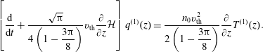 $$\begin{eqnarray}\left[\frac{\text{d}}{\text{d}t}+\frac{\sqrt{\unicode[STIX]{x03C0}}}{4\left(1-{\displaystyle \frac{3\unicode[STIX]{x03C0}}{8}}\right)}v_{\text{th}}\frac{\unicode[STIX]{x2202}}{\unicode[STIX]{x2202}z}{\mathcal{H}}\right]q^{(1)}(z)=\frac{n_{0}v_{\text{th}}^{2}}{2\left(1-{\displaystyle \frac{3\unicode[STIX]{x03C0}}{8}}\right)}\frac{\unicode[STIX]{x2202}}{\unicode[STIX]{x2202}z}T^{(1)}(z).\end{eqnarray}$$
The expression is equal for example to equation (57) in Passot & Sulem (Reference Passot and Sulem2003) for the parallel heat flux
 $q_{\Vert }$
(where in that paper
$q_{\Vert }$
(where in that paper
 $v_{\text{th}}=\sqrt{T^{(0)}/m}$
is used, whereas ours here is
$v_{\text{th}}=\sqrt{T^{(0)}/m}$
is used, whereas ours here is
 $v_{\text{th}}=\sqrt{2T^{(0)}/m}$
).
$v_{\text{th}}=\sqrt{2T^{(0)}/m}$
).
The time-dependent closure (3.280) was obtained with the approximant
 $R_{4,3}(\unicode[STIX]{x1D701})$
. Interestingly, if the derivative
$R_{4,3}(\unicode[STIX]{x1D701})$
. Interestingly, if the derivative
 $\text{d}/\text{d}t$
is neglected, the closure is equivalent to the quasi-static closure (3.261) obtained with
$\text{d}/\text{d}t$
is neglected, the closure is equivalent to the quasi-static closure (3.261) obtained with
 $R_{3,2}(\unicode[STIX]{x1D701})$
(which can be easily seen in Fourier space, or by using
$R_{3,2}(\unicode[STIX]{x1D701})$
(which can be easily seen in Fourier space, or by using
 ${\mathcal{H}}{\mathcal{H}}=-1$
). Also, it is useful to compare the time-dependent (3.280) with the quasi-static closure (3.266), that was obtained for the same approximant
${\mathcal{H}}{\mathcal{H}}=-1$
). Also, it is useful to compare the time-dependent (3.280) with the quasi-static closure (3.266), that was obtained for the same approximant
 $R_{4,3}(\unicode[STIX]{x1D701})$
. To compare these closures, we need to use a time-dependent heat flux equation where the closure for
$R_{4,3}(\unicode[STIX]{x1D701})$
. To compare these closures, we need to use a time-dependent heat flux equation where the closure for
 $\widetilde{r}$
will be applied. In Part 1 of this guide, we derived nonlinear ‘fluid’ equation for the parallel heat flux
$\widetilde{r}$
will be applied. In Part 1 of this guide, we derived nonlinear ‘fluid’ equation for the parallel heat flux
 $q_{\Vert }$
(see Part 1, section ‘Collisionless damping in fluid models – Landau fluid models’). Quickly rewriting it in the 1-D parallel geometry that we use here yields (dropping the parallel subscript)
$q_{\Vert }$
(see Part 1, section ‘Collisionless damping in fluid models – Landau fluid models’). Quickly rewriting it in the 1-D parallel geometry that we use here yields (dropping the parallel subscript)
 $$\begin{eqnarray}\frac{\unicode[STIX]{x2202}q}{\unicode[STIX]{x2202}t}+\unicode[STIX]{x2202}_{z}(qu)+\unicode[STIX]{x2202}_{z}\widetilde{r}+3p\unicode[STIX]{x2202}_{z}\left(\frac{p}{\unicode[STIX]{x1D70C}}\right)+3q\unicode[STIX]{x2202}_{z}u=0,\end{eqnarray}$$
where for brevity
 $\unicode[STIX]{x2202}/\unicode[STIX]{x2202}z=\unicode[STIX]{x2202}_{z}$
. The equation can be of course obtained by direct integration of the 1-D Vlasov equation
$\unicode[STIX]{x2202}/\unicode[STIX]{x2202}z=\unicode[STIX]{x2202}_{z}$
. The equation can be of course obtained by direct integration of the 1-D Vlasov equation
 $\unicode[STIX]{x2202}f/\unicode[STIX]{x2202}t+v\unicode[STIX]{x2202}_{z}f+(q_{r}/m_{r})E\unicode[STIX]{x2202}f/\unicode[STIX]{x2202}v=0$
, as done by Hammett & Perkins (Reference Hammett and Perkins1990), and prescribing a Maxwellian by
$\unicode[STIX]{x2202}f/\unicode[STIX]{x2202}t+v\unicode[STIX]{x2202}_{z}f+(q_{r}/m_{r})E\unicode[STIX]{x2202}f/\unicode[STIX]{x2202}v=0$
, as done by Hammett & Perkins (Reference Hammett and Perkins1990), and prescribing a Maxwellian by
 $r=3p^{2}/\unicode[STIX]{x1D70C}+\widetilde{r}$
. The equation is nonlinear and to compare closures that were done at the linear level, we need to linearize the heat flux equation. This eliminates the second and the last term, the fourth term is linearized as
$r=3p^{2}/\unicode[STIX]{x1D70C}+\widetilde{r}$
. The equation is nonlinear and to compare closures that were done at the linear level, we need to linearize the heat flux equation. This eliminates the second and the last term, the fourth term is linearized as
 $3(p_{0}/m)\unicode[STIX]{x2202}_{z}T^{(1)}$
, and since
$3(p_{0}/m)\unicode[STIX]{x2202}_{z}T^{(1)}$
, and since
 $p_{0}/m=n_{0}v_{\text{th}}^{2}/2$
, the linearized equation reads
$p_{0}/m=n_{0}v_{\text{th}}^{2}/2$
, the linearized equation reads
 $$\begin{eqnarray}\frac{\unicode[STIX]{x2202}q^{(1)}}{\unicode[STIX]{x2202}t}+\unicode[STIX]{x2202}_{z}\widetilde{r}^{(1)}+\frac{3}{2}n_{0}v_{\text{th}}^{2}\unicode[STIX]{x2202}_{z}T^{(1)}=0.\end{eqnarray}$$
This is just a 1-D linear heat flux equation, where no closure was imposed yet. The quantities
 $q^{(1)},\widetilde{r}^{(1)},T^{(1)}$
were not calculated from kinetic theory by using approximants to
$q^{(1)},\widetilde{r}^{(1)},T^{(1)}$
were not calculated from kinetic theory by using approximants to
 $R(\unicode[STIX]{x1D701})$
, etc. The equation was obtained by a general ‘fluid approach’, that we heavily used before we started to consider kinetic calculations (perturbations around a Maxwellian are assumed here because of the prescribed
$R(\unicode[STIX]{x1D701})$
, etc. The equation was obtained by a general ‘fluid approach’, that we heavily used before we started to consider kinetic calculations (perturbations around a Maxwellian are assumed here because of the prescribed
 $r$
). The equation (3.283) greatly clarifies relations between the quasi-static and time-dependent Landau fluid closures. For example, by using the quasi-static closure (3.266) in the heat flux equation (3.283), the time-dependent closure (3.279) is immediately recovered.
$r$
). The equation (3.283) greatly clarifies relations between the quasi-static and time-dependent Landau fluid closures. For example, by using the quasi-static closure (3.266) in the heat flux equation (3.283), the time-dependent closure (3.279) is immediately recovered.
Often, time-dependent closures cannot be straightforwardly constructed by a simple division of two moments, as done above. It is useful to learn a new technique that will allow us to see and construct possible closures in a quicker way. Let us explore the closure (3.276). It is apparent that whenever we attempt to use
 $\unicode[STIX]{x2202}/\unicode[STIX]{x2202}t$
of some moment (in this case
$\unicode[STIX]{x2202}/\unicode[STIX]{x2202}t$
of some moment (in this case
 $\unicode[STIX]{x2202}q^{(1)}/\unicode[STIX]{x2202}t$
), it is logical to also use the same moment without the time derivative (
$\unicode[STIX]{x2202}q^{(1)}/\unicode[STIX]{x2202}t$
), it is logical to also use the same moment without the time derivative (
 $q^{(1)}$
) in the construction of the considered closure, i.e. in this case we search for a closure
$q^{(1)}$
) in the construction of the considered closure, i.e. in this case we search for a closure
 $$\begin{eqnarray}R_{4,3}(\unicode[STIX]{x1D701}):\quad \left(\unicode[STIX]{x1D701}+\unicode[STIX]{x1D6FC}_{q}\right)q^{(1)}=\unicode[STIX]{x1D6FC}_{T}T^{(1)},\end{eqnarray}$$
where
 $\unicode[STIX]{x1D6FC}_{q},\unicode[STIX]{x1D6FC}_{T}$
need to be determined. By using expressions for
$\unicode[STIX]{x1D6FC}_{q},\unicode[STIX]{x1D6FC}_{T}$
need to be determined. By using expressions for
 $q^{(1)},T^{(1)}$
, the above closure is separated to 2 equations for
$q^{(1)},T^{(1)}$
, the above closure is separated to 2 equations for
 $\unicode[STIX]{x1D701}$
and
$\unicode[STIX]{x1D701}$
and
 $\unicode[STIX]{x1D701}^{2}$
that must be satisfied independently if the closure is valid for all
$\unicode[STIX]{x1D701}^{2}$
that must be satisfied independently if the closure is valid for all
 $\unicode[STIX]{x1D701}$
, and solving these 2 equations yields
$\unicode[STIX]{x1D701}$
, and solving these 2 equations yields
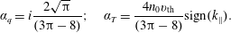 $$\begin{eqnarray}\unicode[STIX]{x1D6FC}_{q}=i\frac{2\sqrt{\unicode[STIX]{x03C0}}}{(3\unicode[STIX]{x03C0}-8)};\quad \unicode[STIX]{x1D6FC}_{T}=\frac{4n_{0}v_{\text{th}}}{(3\unicode[STIX]{x03C0}-8)}\text{sign}(k_{\Vert }).\end{eqnarray}$$
The closure therefore reads
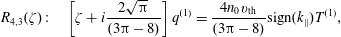 $$\begin{eqnarray}R_{4,3}(\unicode[STIX]{x1D701}):\quad \left[\unicode[STIX]{x1D701}+i\frac{2\sqrt{\unicode[STIX]{x03C0}}}{(3\unicode[STIX]{x03C0}-8)}\right]q^{(1)}=\frac{4n_{0}v_{\text{th}}}{(3\unicode[STIX]{x03C0}-8)}\text{sign}(k_{\Vert })T^{(1)},\end{eqnarray}$$
and is of course equivalent to (3.276).
We are now ready to construct all other possible time-dependent closures. Still considering the
 $R_{4,3}(\unicode[STIX]{x1D701})$
approximant, another possible closure is
$R_{4,3}(\unicode[STIX]{x1D701})$
approximant, another possible closure is
 $$\begin{eqnarray}R_{4,3}(\unicode[STIX]{x1D701}):\quad (\unicode[STIX]{x1D701}+\unicode[STIX]{x1D6FC}_{r})\widetilde{r}^{(1)}=\unicode[STIX]{x1D6FC}_{u}u^{(1)}+\unicode[STIX]{x1D6FC}_{q}q^{(1)},\end{eqnarray}$$
which when separated into 3 equations for
 $\unicode[STIX]{x1D701},\unicode[STIX]{x1D701}^{2}$
and
$\unicode[STIX]{x1D701},\unicode[STIX]{x1D701}^{2}$
and
 $\unicode[STIX]{x1D701}^{3}$
that must each be satisfied yields
$\unicode[STIX]{x1D701}^{3}$
that must each be satisfied yields
 $$\begin{eqnarray}\displaystyle & & \displaystyle \unicode[STIX]{x1D6FC}_{r}=\frac{i16\sqrt{\unicode[STIX]{x03C0}}}{(32-9\unicode[STIX]{x03C0})(3\unicode[STIX]{x03C0}-8)};\quad \unicode[STIX]{x1D6FC}_{u}=\frac{(32-9\unicode[STIX]{x03C0})}{(3\unicode[STIX]{x03C0}-8)}v_{\text{th}}n_{0}T^{(0)}\text{sign}(k_{\Vert });\nonumber\\ \displaystyle & & \displaystyle \qquad \unicode[STIX]{x1D6FC}_{q}=\frac{(81\unicode[STIX]{x03C0}^{2}-552\unicode[STIX]{x03C0}+1024)}{2(32-9\unicode[STIX]{x03C0})(3\unicode[STIX]{x03C0}-8)}v_{\text{th}}\text{sign}(k_{\Vert }),\end{eqnarray}$$
the closure reads
 $$\begin{eqnarray}\displaystyle R_{4,3}(\unicode[STIX]{x1D701}):\quad \left[-i\unicode[STIX]{x1D714}+\frac{16\sqrt{\unicode[STIX]{x03C0}}}{(32-9\unicode[STIX]{x03C0})(3\unicode[STIX]{x03C0}-8)}v_{\text{th}}|k_{\Vert }|\right]\widetilde{r}^{(1)} & = & \displaystyle -\frac{(32-9\unicode[STIX]{x03C0})}{(3\unicode[STIX]{x03C0}-8)}v_{\text{th}}^{2}n_{0}T^{(0)}ik_{\Vert }u^{(1)}-\frac{(81\unicode[STIX]{x03C0}^{2}-552\unicode[STIX]{x03C0}+1024)}{2(32-9\unicode[STIX]{x03C0})(3\unicode[STIX]{x03C0}-8)}v_{\text{th}}^{2}ik_{\Vert }q^{(1)};\nonumber\\ \displaystyle \left[\frac{\text{d}}{\text{d}t}-\frac{16\sqrt{\unicode[STIX]{x03C0}}}{(32-9\unicode[STIX]{x03C0})(3\unicode[STIX]{x03C0}-8)}v_{\text{th}}\unicode[STIX]{x2202}_{z}{\mathcal{H}}\right]\widetilde{r}^{(1)} & = & \displaystyle -\frac{(32-9\unicode[STIX]{x03C0})}{(3\unicode[STIX]{x03C0}-8)}v_{\text{th}}^{2}n_{0}T^{(0)}\unicode[STIX]{x2202}_{z}u^{(1)}-\frac{(81\unicode[STIX]{x03C0}^{2}-552\unicode[STIX]{x03C0}+1024)}{2(32-9\unicode[STIX]{x03C0})(3\unicode[STIX]{x03C0}-8)}v_{\text{th}}^{2}\unicode[STIX]{x2202}_{z}q^{(1)},\nonumber\\ \displaystyle & & \displaystyle\end{eqnarray}$$
and this closure will be eliminated.
Another closure with
 $R_{4,3}(\unicode[STIX]{x1D701})$
can be constructed as
$R_{4,3}(\unicode[STIX]{x1D701})$
can be constructed as

so the closure reads
 $$\begin{eqnarray}\displaystyle R_{4,3}(\unicode[STIX]{x1D701}):\quad -i\unicode[STIX]{x1D714}\widetilde{r}^{(1)} & = & \displaystyle -\frac{(32-9\unicode[STIX]{x03C0})}{(3\unicode[STIX]{x03C0}-8)}v_{\text{th}}^{2}n_{0}T^{(0)}ik_{\Vert }u^{(1)}-\frac{8\sqrt{\unicode[STIX]{x03C0}}}{(3\unicode[STIX]{x03C0}-8)^{2}}v_{\text{th}}^{3}n_{0}|k_{\Vert }|T^{(1)}+\frac{(27\unicode[STIX]{x03C0}^{2}-160\unicode[STIX]{x03C0}+256)}{2(3\unicode[STIX]{x03C0}-8)^{2}}v_{\text{th}}^{2}ik_{\Vert }q^{(1)};\nonumber\\ \displaystyle \frac{\text{d}}{\text{d}t}\widetilde{r}^{(1)} & = & \displaystyle -\frac{(32-9\unicode[STIX]{x03C0})}{(3\unicode[STIX]{x03C0}-8)}v_{\text{th}}^{2}n_{0}T^{(0)}\unicode[STIX]{x2202}_{z}u^{(1)}+\frac{8\sqrt{\unicode[STIX]{x03C0}}}{(3\unicode[STIX]{x03C0}-8)^{2}}v_{\text{th}}^{3}n_{0}\unicode[STIX]{x2202}_{z}{\mathcal{H}}T^{(1)}+\frac{(27\unicode[STIX]{x03C0}^{2}-160\unicode[STIX]{x03C0}+256)}{2(3\unicode[STIX]{x03C0}-8)^{2}}v_{\text{th}}^{2}\unicode[STIX]{x2202}_{z}q^{(1)},\nonumber\\ \displaystyle & & \displaystyle\end{eqnarray}$$
and this closure will be eliminated as well. The time-dependent closures (3.290) and (3.287) are of course closely related, and one can go from one to another by using the quasi-static closure (3.266) that expresses
 $\widetilde{r}^{(1)}$
as a combination of
$\widetilde{r}^{(1)}$
as a combination of
 $T^{(1)}$
and
$T^{(1)}$
and
 $q^{(1)}$
.
$q^{(1)}$
.
Continuing with the
 $R_{4,2}(\unicode[STIX]{x1D701})$
approximant, it is possible to construct the following closure
$R_{4,2}(\unicode[STIX]{x1D701})$
approximant, it is possible to construct the following closure

that implies
 $$\begin{eqnarray}\left[-i\unicode[STIX]{x1D714}+\sqrt{\unicode[STIX]{x03C0}}\frac{10-3\unicode[STIX]{x03C0}}{16-5\unicode[STIX]{x03C0}}v_{\text{th}}|k_{\Vert }|\right]q^{(1)}=-n_{0}v_{\text{th}}^{2}\frac{3\unicode[STIX]{x03C0}-8}{16-5\unicode[STIX]{x03C0}}ik_{\Vert }T^{(1)}+n_{0}T^{(0)}v_{\text{th}}\sqrt{\unicode[STIX]{x03C0}}\frac{9\unicode[STIX]{x03C0}-28}{16-5\unicode[STIX]{x03C0}}|k_{\Vert }|u^{(1)};\end{eqnarray}$$
and the result is consistent with using the quasi-static closure (3.267) in the linearized heat flux equation (3.283).
Continuing with
 $R_{4,4}(\unicode[STIX]{x1D701})$
, it is possible to construct
$R_{4,4}(\unicode[STIX]{x1D701})$
, it is possible to construct

and the closure reads
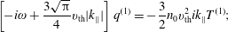 $$\begin{eqnarray}\left[-i\unicode[STIX]{x1D714}+\frac{3\sqrt{\unicode[STIX]{x03C0}}}{4}v_{\text{th}}|k_{\Vert }|\right]q^{(1)}=-\frac{3}{2}n_{0}v_{\text{th}}^{2}ik_{\Vert }T^{(1)};\end{eqnarray}$$
The obtained closure is related to the quasi-static closure (3.268), since by using the quasi-static closure (3.268) in the linear heat flux equation (3.283), the time-dependent closure (3.295) is recovered.
Another closure with
 $R_{4,4}(\unicode[STIX]{x1D701})$
is
$R_{4,4}(\unicode[STIX]{x1D701})$
is

And yet another closure with
 $R_{4,4}(\unicode[STIX]{x1D701})$
 $$\begin{eqnarray}\displaystyle & & \displaystyle R_{4,4}(\unicode[STIX]{x1D701}):\quad \unicode[STIX]{x1D701}\widetilde{r}^{(1)}=\unicode[STIX]{x1D6FC}_{T}T^{(1)}+\unicode[STIX]{x1D6FC}_{q}q^{(1)};\end{eqnarray}$$
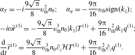 $$\begin{eqnarray}\displaystyle & & \displaystyle \unicode[STIX]{x1D6FC}_{T}=-i\frac{9\sqrt{\unicode[STIX]{x03C0}}}{8}v_{\text{th}}^{2}n_{0};\quad \unicode[STIX]{x1D6FC}_{q}=-\frac{9\unicode[STIX]{x03C0}}{16}v_{\text{th}}\text{sign}(k_{\Vert });\nonumber\\ \displaystyle & & \displaystyle -i\unicode[STIX]{x1D714}\widetilde{r}^{(1)}=-\frac{9\sqrt{\unicode[STIX]{x03C0}}}{8}v_{\text{th}}^{3}n_{0}|k_{\Vert }|T^{(1)}+\frac{9\unicode[STIX]{x03C0}}{16}v_{\text{th}}^{2}ik_{\Vert }q^{(1)};\nonumber\\ \displaystyle & & \displaystyle \frac{\text{d}}{\text{d}t}\widetilde{r}^{(1)}=\frac{9\sqrt{\unicode[STIX]{x03C0}}}{8}v_{\text{th}}^{3}n_{0}\unicode[STIX]{x2202}_{z}{\mathcal{H}}T^{(1)}+\frac{9\unicode[STIX]{x03C0}}{16}v_{\text{th}}^{2}\unicode[STIX]{x2202}_{z}q^{(1)}.\end{eqnarray}$$
The closure (3.299) is related to the closure (3.297), because one can use the quasi-static closure (3.268) to express
 $\widetilde{r}^{(1)}$
through
$\widetilde{r}^{(1)}$
through
 $q^{(1)}$
, however, the closure (3.299) will be eliminated.
$q^{(1)}$
, however, the closure (3.299) will be eliminated.
The
 $R_{4,5}(\unicode[STIX]{x1D701})$
was eliminated because it is not a well-behaved approximant (see discussion above), nevertheless, for completeness the following closure can be constructed
$R_{4,5}(\unicode[STIX]{x1D701})$
was eliminated because it is not a well-behaved approximant (see discussion above), nevertheless, for completeness the following closure can be constructed

With
 $R_{3,2}(\unicode[STIX]{x1D701})$
, the following time-dependent closure can be constructed
$R_{3,2}(\unicode[STIX]{x1D701})$
, the following time-dependent closure can be constructed

and similarly, yet another one
 $$\begin{eqnarray}\displaystyle & & \displaystyle R_{3,2}(\unicode[STIX]{x1D701}):\quad \unicode[STIX]{x1D701}q^{(1)}=\unicode[STIX]{x1D6FC}_{u}u^{(1)}+\unicode[STIX]{x1D6FC}_{T}T^{(1)};\end{eqnarray}$$
 $$\begin{eqnarray}\displaystyle & & \displaystyle \unicode[STIX]{x1D6FC}_{u}=-\frac{4i}{\sqrt{\unicode[STIX]{x03C0}}}n_{0}T^{(0)};\quad \unicode[STIX]{x1D6FC}_{T}=-\frac{4}{\unicode[STIX]{x03C0}}n_{0}v_{\text{th}}\text{sign}(k_{\Vert });\nonumber\\ \displaystyle & & \displaystyle -i\unicode[STIX]{x1D714}q^{(1)}=-\frac{4}{\sqrt{\unicode[STIX]{x03C0}}}n_{0}T^{(0)}v_{\text{th}}|k_{\Vert }|u^{(1)}+\frac{4}{\unicode[STIX]{x03C0}}n_{0}v_{\text{th}}^{2}ik_{\Vert }T^{(1)};\nonumber\\ \displaystyle & & \displaystyle \frac{\text{d}}{\text{d}t}q^{(1)}=+\frac{4}{\sqrt{\unicode[STIX]{x03C0}}}n_{0}T^{(0)}v_{\text{th}}\unicode[STIX]{x2202}_{z}{\mathcal{H}}u^{(1)}+\frac{4}{\unicode[STIX]{x03C0}}n_{0}v_{\text{th}}^{2}\unicode[STIX]{x2202}_{z}T^{(1)},\end{eqnarray}$$
however, the last closure will be eliminated.
3.11 Time-dependent closures with five-pole approximants
Now we can use this technique to construct time-dependent closures with five-pole approximants of
 $R(\unicode[STIX]{x1D701})$
. Starting with the
$R(\unicode[STIX]{x1D701})$
. Starting with the
 $R_{5,4}(\unicode[STIX]{x1D701})$
approximant
$R_{5,4}(\unicode[STIX]{x1D701})$
approximant
 $$\begin{eqnarray}R_{5,4}(\unicode[STIX]{x1D701})=\frac{1+a_{1}\unicode[STIX]{x1D701}+a_{2}\unicode[STIX]{x1D701}^{2}+a_{3}\unicode[STIX]{x1D701}^{3}}{1+3(a_{1}+a_{3})\unicode[STIX]{x1D701}+(3a_{2}-2)\unicode[STIX]{x1D701}^{2}+(3a_{3}-2a_{1})\unicode[STIX]{x1D701}^{3}-2a_{2}\unicode[STIX]{x1D701}^{4}-2a_{3}\unicode[STIX]{x1D701}^{5}},\end{eqnarray}$$
where the constants
 $a_{1},a_{2},a_{3}$
are given in (A 8), the kinetic moments calculate as
$a_{1},a_{2},a_{3}$
are given in (A 8), the kinetic moments calculate as
 $$\begin{eqnarray}\displaystyle R_{5,4}(\unicode[STIX]{x1D701}):\quad D & = & \displaystyle \left(1+3(a_{1}+a_{3})\unicode[STIX]{x1D701}+(3a_{2}-2)\unicode[STIX]{x1D701}^{2}+(3a_{3}-2a_{1})\unicode[STIX]{x1D701}^{3}-2a_{2}\unicode[STIX]{x1D701}^{4}-2a_{3}\unicode[STIX]{x1D701}^{5}\right);\nonumber\\ \displaystyle & & \displaystyle\end{eqnarray}$$
 $$\begin{eqnarray}\displaystyle u^{(1)} & = & \displaystyle -\frac{q_{r}}{T^{(0)}}\unicode[STIX]{x1D6F7}v_{\text{th}}\text{sign}(k_{\Vert })\frac{1}{D}\left[a_{3}\unicode[STIX]{x1D701}^{4}+a_{2}\unicode[STIX]{x1D701}^{3}+a_{1}\unicode[STIX]{x1D701}^{2}+\unicode[STIX]{x1D701}\right];\end{eqnarray}$$
 $$\begin{eqnarray}\displaystyle T^{(1)} & = & \displaystyle -q_{r}\unicode[STIX]{x1D6F7}\frac{1}{D}\left[2a_{3}\unicode[STIX]{x1D701}^{3}+2a_{2}\unicode[STIX]{x1D701}^{2}+(2a_{1}+3a_{3})\unicode[STIX]{x1D701}\right];\end{eqnarray}$$
 $$\begin{eqnarray}\displaystyle q^{(1)} & = & \displaystyle -q_{r}n_{0}\unicode[STIX]{x1D6F7}v_{\text{th}}\text{sign}(k_{\Vert })\frac{1}{D}\left[3a_{3}\unicode[STIX]{x1D701}^{2}-2\unicode[STIX]{x1D701}\right];\end{eqnarray}$$
 $$\begin{eqnarray}\displaystyle \widetilde{r}^{(1)} & = & \displaystyle -q_{r}\frac{n_{0}}{2}v_{\text{th}}^{2}\unicode[STIX]{x1D6F7}\frac{1}{D}\left[-(6a_{2}+4)\unicode[STIX]{x1D701}^{2}-(6a_{1}+9a_{3})\unicode[STIX]{x1D701}\right].\end{eqnarray}$$
It is possible to construct time-dependent closure for
 $\widetilde{r}^{(1)}$
, by searching for a solution
$\widetilde{r}^{(1)}$
, by searching for a solution
 $$\begin{eqnarray}(\unicode[STIX]{x1D701}+\unicode[STIX]{x1D6FC}_{r})\widetilde{r}^{(1)}=\unicode[STIX]{x1D6FC}_{T}T^{(1)}+\unicode[STIX]{x1D6FC}_{q}q^{(1)}.\end{eqnarray}$$
Separating the equation to 3 equations for
 $\unicode[STIX]{x1D701},\unicode[STIX]{x1D701}^{2},\unicode[STIX]{x1D701}^{3}$
, the solution is
$\unicode[STIX]{x1D701},\unicode[STIX]{x1D701}^{2},\unicode[STIX]{x1D701}^{3}$
, the solution is
 $$\begin{eqnarray}\unicode[STIX]{x1D6FC}_{r}=\frac{a_{2}}{a_{3}};\quad \unicode[STIX]{x1D6FC}_{T}=-n_{0}v_{\text{th}}^{2}\frac{3a_{2}+2}{2a_{3}};\quad \unicode[STIX]{x1D6FC}_{q}=-v_{\text{th}}\text{sign}(k_{\Vert })\frac{2a_{1}+3a_{3}}{2a_{3}},\end{eqnarray}$$
that evaluates as
 $$\begin{eqnarray}\unicode[STIX]{x1D6FC}_{r}=i\frac{21\unicode[STIX]{x03C0}-64}{\sqrt{\unicode[STIX]{x03C0}}(9\unicode[STIX]{x03C0}-28)};\quad \unicode[STIX]{x1D6FC}_{T}=in_{0}v_{\text{th}}^{2}\frac{256-81\unicode[STIX]{x03C0}}{2(9\unicode[STIX]{x03C0}-28)\sqrt{\unicode[STIX]{x03C0}}};\quad \unicode[STIX]{x1D6FC}_{q}=v_{\text{th}}\text{sign}(k_{\Vert })\frac{32-9\unicode[STIX]{x03C0}}{2(9\unicode[STIX]{x03C0}-28)}.\end{eqnarray}$$
The
 $R_{5,4}(\unicode[STIX]{x1D701})$
closure therefore reads
$R_{5,4}(\unicode[STIX]{x1D701})$
closure therefore reads
 $$\begin{eqnarray}\left[-i\unicode[STIX]{x1D714}+\frac{21\unicode[STIX]{x03C0}-64}{\sqrt{\unicode[STIX]{x03C0}}(9\unicode[STIX]{x03C0}-28)}v_{\text{th}}|k_{\Vert }|\right]\widetilde{r}^{(1)}=n_{0}v_{\text{th}}^{3}\frac{256-81\unicode[STIX]{x03C0}}{2(9\unicode[STIX]{x03C0}-28)\sqrt{\unicode[STIX]{x03C0}}}|k_{\Vert }|T^{(1)}-v_{\text{th}}^{2}\frac{32-9\unicode[STIX]{x03C0}}{2(9\unicode[STIX]{x03C0}-28)}ik_{\Vert }q^{(1)},\end{eqnarray}$$
and transformation to real space yields
The closure is interesting, since the
 $R_{5,4}(\unicode[STIX]{x1D701})$
is a very precise
$R_{5,4}(\unicode[STIX]{x1D701})$
is a very precise
 $o(\unicode[STIX]{x1D701}^{3})$
,
$o(\unicode[STIX]{x1D701}^{3})$
,
 $o(1/\unicode[STIX]{x1D701}^{6})$
approximant, and it is therefore only one of two closures that have precision
$o(1/\unicode[STIX]{x1D701}^{6})$
approximant, and it is therefore only one of two closures that have precision
 $o(\unicode[STIX]{x1D701}^{3})$
. For large
$o(\unicode[STIX]{x1D701}^{3})$
. For large
 $\unicode[STIX]{x1D701}$
, the moments have correct asymptotic behaviour up to the heat flux
$\unicode[STIX]{x1D701}$
, the moments have correct asymptotic behaviour up to the heat flux
 $q^{(1)}\sim -3/(2\unicode[STIX]{x1D701}^{3})$
(including the proportionality constant) and the
$q^{(1)}\sim -3/(2\unicode[STIX]{x1D701}^{3})$
(including the proportionality constant) and the
 $\widetilde{r}^{(1)}\sim 1/\unicode[STIX]{x1D701}^{3}$
, which is not bad either. Additionally, the closure does not contain
$\widetilde{r}^{(1)}\sim 1/\unicode[STIX]{x1D701}^{3}$
, which is not bad either. Additionally, the closure does not contain
 $u^{(1)}$
, which is advantageous.
$u^{(1)}$
, which is advantageous.
Constructing a closure with
 $R_{5,5}(\unicode[STIX]{x1D701})$
is done quickly, by using
$R_{5,5}(\unicode[STIX]{x1D701})$
is done quickly, by using
 $a_{2}=-2/3$
in the kinetic moments for
$a_{2}=-2/3$
in the kinetic moments for
 $R_{5,4}(\unicode[STIX]{x1D701})$
, so
$R_{5,4}(\unicode[STIX]{x1D701})$
, so
 $$\begin{eqnarray}\displaystyle R_{5,5}(\unicode[STIX]{x1D701}):\quad D & = & \displaystyle \left(1+3(a_{1}+a_{3})\unicode[STIX]{x1D701}-4\unicode[STIX]{x1D701}^{2}+(3a_{3}-2a_{1})\unicode[STIX]{x1D701}^{3}+{\textstyle \frac{4}{3}}\unicode[STIX]{x1D701}^{4}-2a_{3}\unicode[STIX]{x1D701}^{5}\right);\nonumber\\ \displaystyle & & \displaystyle\end{eqnarray}$$
 $$\begin{eqnarray}\displaystyle q^{(1)} & = & \displaystyle -q_{r}n_{0}\unicode[STIX]{x1D6F7}v_{\text{th}}\text{sign}(k_{\Vert })\frac{1}{D}\left[i\frac{(32-9\unicode[STIX]{x03C0})}{3\sqrt{\unicode[STIX]{x03C0}}}\unicode[STIX]{x1D701}^{2}-2\unicode[STIX]{x1D701}\right];\end{eqnarray}$$
 $$\begin{eqnarray}\displaystyle \widetilde{r}^{(1)} & = & \displaystyle -q_{r}\frac{n_{0}}{2}v_{\text{th}}^{2}\unicode[STIX]{x1D6F7}\frac{1}{D}[3i\sqrt{\unicode[STIX]{x03C0}}\unicode[STIX]{x1D701}],\end{eqnarray}$$
where
 $a_{1},a_{3}$
are given in (A 9). Searching for a closure
$a_{1},a_{3}$
are given in (A 9). Searching for a closure
 $(\unicode[STIX]{x1D701}+\unicode[STIX]{x1D6FC}_{r})\widetilde{r}^{(1)}=\unicode[STIX]{x1D6FC}_{q}q^{(1)}$
has a solution
$(\unicode[STIX]{x1D701}+\unicode[STIX]{x1D6FC}_{r})\widetilde{r}^{(1)}=\unicode[STIX]{x1D6FC}_{q}q^{(1)}$
has a solution

and the closure in real space reads
The
 $R_{5,5}(\unicode[STIX]{x1D701})$
approximant has precision
$R_{5,5}(\unicode[STIX]{x1D701})$
approximant has precision
 $o(\unicode[STIX]{x1D701}^{2})$
,
$o(\unicode[STIX]{x1D701}^{2})$
,
 $o(1/\unicode[STIX]{x1D701}^{7})$
. The increase of the asymptotic precision reproduces the correct asymptote
$o(1/\unicode[STIX]{x1D701}^{7})$
. The increase of the asymptotic precision reproduces the correct asymptote
 $\widetilde{r}^{(1)}\sim 1/\unicode[STIX]{x1D701}^{4}$
, even though with proportionality constant
$\widetilde{r}^{(1)}\sim 1/\unicode[STIX]{x1D701}^{4}$
, even though with proportionality constant
 $\widetilde{r}^{(1)}\sim -(27\unicode[STIX]{x03C0}/2(32-9\unicode[STIX]{x03C0})\unicode[STIX]{x1D701}^{4})=-11.38/\unicode[STIX]{x1D701}^{4}$
instead of the correct
$\widetilde{r}^{(1)}\sim -(27\unicode[STIX]{x03C0}/2(32-9\unicode[STIX]{x03C0})\unicode[STIX]{x1D701}^{4})=-11.38/\unicode[STIX]{x1D701}^{4}$
instead of the correct
 $-6/\unicode[STIX]{x1D701}^{4}$
.
$-6/\unicode[STIX]{x1D701}^{4}$
.
Continuing with the approximant
 $R_{5,6}(\unicode[STIX]{x1D701})$
, the kinetic moments calculate as
$R_{5,6}(\unicode[STIX]{x1D701})$
, the kinetic moments calculate as
 $$\begin{eqnarray}\displaystyle R_{5,6}(\unicode[STIX]{x1D701}):\quad D & = & \displaystyle \left(1-i\sqrt{\unicode[STIX]{x03C0}}\frac{15}{8}\unicode[STIX]{x1D701}-4\unicode[STIX]{x1D701}^{2}+i\sqrt{\unicode[STIX]{x03C0}}\frac{5}{2}\unicode[STIX]{x1D701}^{3}+\frac{4}{3}\unicode[STIX]{x1D701}^{4}-i\frac{\sqrt{\unicode[STIX]{x03C0}}}{2}\unicode[STIX]{x1D701}^{5}\right);\end{eqnarray}$$
 $$\begin{eqnarray}\displaystyle q^{(1)} & = & \displaystyle -q_{r}n_{0}\unicode[STIX]{x1D6F7}v_{\text{th}}\text{sign}(k_{\Vert })\frac{1}{D}\left[\frac{3i\sqrt{\unicode[STIX]{x03C0}}}{4}\unicode[STIX]{x1D701}^{2}-2\unicode[STIX]{x1D701}\right];\end{eqnarray}$$
 $$\begin{eqnarray}\displaystyle \widetilde{r}^{(1)} & = & \displaystyle -q_{r}\frac{n_{0}}{2}v_{\text{th}}^{2}\unicode[STIX]{x1D6F7}\frac{1}{D}\left[3i\sqrt{\unicode[STIX]{x03C0}}\unicode[STIX]{x1D701}\right],\end{eqnarray}$$
which yields a closure
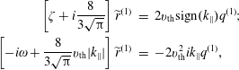
that in real space reads
The
 $R_{5,6}(\unicode[STIX]{x1D701})$
approximant has precision
$R_{5,6}(\unicode[STIX]{x1D701})$
approximant has precision
 $o(\unicode[STIX]{x1D701})$
,
$o(\unicode[STIX]{x1D701})$
,
 $o(1/\unicode[STIX]{x1D701}^{8})$
. Even though the precision for small
$o(1/\unicode[STIX]{x1D701}^{8})$
. Even though the precision for small
 $\unicode[STIX]{x1D701}$
is relatively low, the closure correctly reproduces the asymptotic behaviour
$\unicode[STIX]{x1D701}$
is relatively low, the closure correctly reproduces the asymptotic behaviour
 $\widetilde{r}^{(1)}\sim -6/\unicode[STIX]{x1D701}^{4}$
(including the proportionality constant).
$\widetilde{r}^{(1)}\sim -6/\unicode[STIX]{x1D701}^{4}$
(including the proportionality constant).
Finally, it is indeed possible to construct a closure with precision
 $o(\unicode[STIX]{x1D701}^{4})$
, by using
$o(\unicode[STIX]{x1D701}^{4})$
, by using
 $R_{5,3}(\unicode[STIX]{x1D701})$
. The approximant
$R_{5,3}(\unicode[STIX]{x1D701})$
. The approximant
 $R_{5,3}(\unicode[STIX]{x1D701})$
is defined as
$R_{5,3}(\unicode[STIX]{x1D701})$
is defined as
 $$\begin{eqnarray}R_{5,3}(\unicode[STIX]{x1D701})=\frac{1+a_{1}\unicode[STIX]{x1D701}+a_{2}\unicode[STIX]{x1D701}^{2}+a_{3}\unicode[STIX]{x1D701}^{3}}{1+b_{1}\unicode[STIX]{x1D701}+(3a_{2}-2)\unicode[STIX]{x1D701}^{2}+(3a_{3}-2a_{1})\unicode[STIX]{x1D701}^{3}-2a_{2}\unicode[STIX]{x1D701}^{4}-2a_{3}\unicode[STIX]{x1D701}^{5}},\end{eqnarray}$$
where the constants
 $a_{1},a_{2},a_{3},b_{1}$
are given in (A 7). Using this approximant, the kinetic moments calculate as
$a_{1},a_{2},a_{3},b_{1}$
are given in (A 7). Using this approximant, the kinetic moments calculate as
 $$\begin{eqnarray}\displaystyle R_{5,3}(\unicode[STIX]{x1D701}):\quad D & = & \displaystyle \left(1+b_{1}\unicode[STIX]{x1D701}+(3a_{2}-2)\unicode[STIX]{x1D701}^{2}+(3a_{3}-2a_{1})\unicode[STIX]{x1D701}^{3}-2a_{2}\unicode[STIX]{x1D701}^{4}-2a_{3}\unicode[STIX]{x1D701}^{5}\right);\end{eqnarray}$$
 $$\begin{eqnarray}\displaystyle u^{(1)} & = & \displaystyle -\frac{q_{r}}{T^{(0)}}\unicode[STIX]{x1D6F7}v_{\text{th}}\text{sign}(k_{\Vert })\frac{1}{D}\left[a_{3}\unicode[STIX]{x1D701}^{4}+a_{2}\unicode[STIX]{x1D701}^{3}+a_{1}\unicode[STIX]{x1D701}^{2}+\unicode[STIX]{x1D701}\right];\end{eqnarray}$$
 $$\begin{eqnarray}\displaystyle T^{(1)} & = & \displaystyle -q_{r}\unicode[STIX]{x1D6F7}\frac{1}{D}\left[2a_{3}\unicode[STIX]{x1D701}^{3}+2a_{2}\unicode[STIX]{x1D701}^{2}+(b_{1}-a_{1})\unicode[STIX]{x1D701}\right];\end{eqnarray}$$
 $$\begin{eqnarray}\displaystyle q^{(1)} & = & \displaystyle -q_{r}n_{0}\unicode[STIX]{x1D6F7}v_{\text{th}}\text{sign}(k_{\Vert })\frac{1}{D}\left[(b_{1}-3a_{1})\unicode[STIX]{x1D701}^{2}-2\unicode[STIX]{x1D701}\right];\end{eqnarray}$$
 $$\begin{eqnarray}\displaystyle \widetilde{r}^{(1)} & = & \displaystyle -q_{r}\frac{n_{0}}{2}v_{\text{th}}^{2}\unicode[STIX]{x1D6F7}\frac{1}{D}\left[(2b_{1}-6a_{1}-6a_{3})\unicode[STIX]{x1D701}^{3}-(6a_{2}+4)\unicode[STIX]{x1D701}^{2}+(3a_{1}-3b_{1})\unicode[STIX]{x1D701}\right].\nonumber\\ \displaystyle & & \displaystyle\end{eqnarray}$$
It is possible to search for a closure
 $$\begin{eqnarray}R_{5,3}(\unicode[STIX]{x1D701}):\quad \left(\unicode[STIX]{x1D701}+\unicode[STIX]{x1D6FC}_{r}\right)\widetilde{r}^{(1)}=\unicode[STIX]{x1D6FC}_{u}u^{(1)}+\unicode[STIX]{x1D6FC}_{T}T^{(1)}+\unicode[STIX]{x1D6FC}_{q}q^{(1)},\end{eqnarray}$$
and the solution is
 $$\begin{eqnarray}\displaystyle \unicode[STIX]{x1D6FC}_{r} & = & \displaystyle \frac{a_{2}}{a_{3}};\quad \unicode[STIX]{x1D6FC}_{u}=-v_{\text{th}}n_{0}T^{(0)}\frac{(3a_{1}+3a_{3}-b_{1})}{a_{3}}\text{sign}(k_{\Vert });\nonumber\\ \displaystyle \unicode[STIX]{x1D6FC}_{T} & = & \displaystyle -n_{0}v_{\text{th}}^{2}\frac{(3a_{2}+2)}{2a_{3}};\quad \unicode[STIX]{x1D6FC}_{q}=-v_{\text{th}}\frac{(2a_{1}+3a_{3})}{2a_{3}}\text{sign}(k_{\Vert }).\end{eqnarray}$$
The correctness of the algebra can be quickly checked by prescribing
 $b_{1}=3a_{1}+3a_{3}$
, which immediately recovers the closure (3.311)–(3.312) that was obtained for
$b_{1}=3a_{1}+3a_{3}$
, which immediately recovers the closure (3.311)–(3.312) that was obtained for
 $R_{5,4}(\unicode[STIX]{x1D701})$
with only asymptotic expansion coefficients (and the power-series coefficients unspecified), which yields
$R_{5,4}(\unicode[STIX]{x1D701})$
with only asymptotic expansion coefficients (and the power-series coefficients unspecified), which yields
 $\unicode[STIX]{x1D6FC}_{u}=0$
. The
$\unicode[STIX]{x1D6FC}_{u}=0$
. The
 $R_{5,3}(\unicode[STIX]{x1D701})$
closure reads
$R_{5,3}(\unicode[STIX]{x1D701})$
closure reads
 $$\begin{eqnarray}\displaystyle R_{5,3}(\unicode[STIX]{x1D701}):\quad \left[-i\unicode[STIX]{x1D714}-i\frac{a_{2}}{a_{3}}v_{\text{th}}|k_{\Vert }|\right]\widetilde{r}^{(1)} & = & \displaystyle v_{\text{th}}^{2}n_{0}T^{(0)}\frac{(3a_{1}+3a_{3}-b_{1})}{a_{3}}ik_{\Vert }u^{(1)}\nonumber\\ \displaystyle & & \displaystyle +\,in_{0}v_{\text{th}}^{3}\frac{(3a_{2}+2)}{2a_{3}}|k_{\Vert }|T^{(1)}+v_{\text{th}}^{2}\frac{(2a_{1}+3a_{3})}{2a_{3}}ik_{\Vert }q^{(1)}.\nonumber\\ \displaystyle & & \displaystyle\end{eqnarray}$$
By using the calculated coefficients from (A 7),
 $$\begin{eqnarray}\displaystyle & & \displaystyle \frac{a_{2}}{a_{3}}=i\frac{(104-33\unicode[STIX]{x03C0})\sqrt{\unicode[STIX]{x03C0}}}{2(9\unicode[STIX]{x03C0}^{2}-69\unicode[STIX]{x03C0}+128)}\equiv i\widetilde{\unicode[STIX]{x1D6FC}}_{r};\quad \!\frac{3a_{1}+3a_{3}-b_{1}}{a_{3}}=\frac{(135\unicode[STIX]{x03C0}^{2}-750\unicode[STIX]{x03C0}+1024)}{2(9\unicode[STIX]{x03C0}^{2}-69\unicode[STIX]{x03C0}+128)}\equiv \widetilde{\unicode[STIX]{x1D6FC}}_{u};\nonumber\\ \displaystyle & & \displaystyle \frac{3a_{2}+2}{2a_{3}}=i\frac{3(160-51\unicode[STIX]{x03C0})\sqrt{\unicode[STIX]{x03C0}}}{4(9\unicode[STIX]{x03C0}^{2}-69\unicode[STIX]{x03C0}+128)}\equiv i\widetilde{\unicode[STIX]{x1D6FC}}_{T};\quad \!\frac{2a_{1}+3a_{3}}{2a_{3}}=\frac{(54\unicode[STIX]{x03C0}^{2}-333\unicode[STIX]{x03C0}+512)}{2(9\unicode[STIX]{x03C0}^{2}-69\unicode[STIX]{x03C0}+128)}\equiv \widetilde{\unicode[STIX]{x1D6FC}}_{q},\nonumber\\ \displaystyle & & \displaystyle\end{eqnarray}$$
the closure in Fourier and real space then reads
 $$\begin{eqnarray}\displaystyle R_{5,3}(\unicode[STIX]{x1D701}):\quad \left[-i\unicode[STIX]{x1D714}+\widetilde{\unicode[STIX]{x1D6FC}}_{r}v_{\text{th}}|k_{\Vert }|\right]\widetilde{r}^{(1)} & = & \displaystyle v_{\text{th}}^{2}n_{0}T^{(0)}\widetilde{\unicode[STIX]{x1D6FC}}_{u}ik_{\Vert }u^{(1)}-n_{0}v_{\text{th}}^{3}\widetilde{\unicode[STIX]{x1D6FC}}_{T}|k_{\Vert }|T^{(1)}+v_{\text{th}}^{2}\widetilde{\unicode[STIX]{x1D6FC}}_{q}ik_{\Vert }q^{(1)};\nonumber\\ \displaystyle & & \displaystyle\end{eqnarray}$$
 $$\begin{eqnarray}\displaystyle \left[\frac{\text{d}}{\text{d}t}-\widetilde{\unicode[STIX]{x1D6FC}}_{r}v_{\text{th}}\unicode[STIX]{x2202}_{z}{\mathcal{H}}\right]\widetilde{r}^{(1)} & = & \displaystyle v_{\text{th}}^{2}n_{0}T^{(0)}\widetilde{\unicode[STIX]{x1D6FC}}_{u}\unicode[STIX]{x2202}_{z}u^{(1)}+n_{0}v_{\text{th}}^{3}\widetilde{\unicode[STIX]{x1D6FC}}_{T}\unicode[STIX]{x2202}_{z}{\mathcal{H}}T^{(1)}+v_{\text{th}}^{2}\widetilde{\unicode[STIX]{x1D6FC}}_{q}\unicode[STIX]{x2202}_{z}q^{(1)},\nonumber\\ \displaystyle & & \displaystyle\end{eqnarray}$$
where the perhaps complicated appearing proportionality constants (that come from the Padé approximation) are just constants, that are numerically evaluated as
 $$\begin{eqnarray}\displaystyle \widetilde{\unicode[STIX]{x1D6FC}}_{r}=5.13185;\quad \widetilde{\unicode[STIX]{x1D6FC}}_{u}=1.78706;\quad \widetilde{\unicode[STIX]{x1D6FC}}_{T}=-5.20074;\quad \widetilde{\unicode[STIX]{x1D6FC}}_{q}=-10.53748. & & \displaystyle\end{eqnarray}$$
For numerical simulations, we of course recommend to re-calculate these constants from the above analytic expressions, to fully match the numerical precision of the considered simulation. For complete clarity, the fully expressed closure in real space reads
 $$\begin{eqnarray}\displaystyle & \displaystyle R_{5,3}(\unicode[STIX]{x1D701}):\quad \left[\frac{\text{d}}{\text{d}t}-\frac{(104-33\unicode[STIX]{x03C0})\sqrt{\unicode[STIX]{x03C0}}}{2(9\unicode[STIX]{x03C0}^{2}-69\unicode[STIX]{x03C0}+128)}v_{\text{th}}\unicode[STIX]{x2202}_{z}{\mathcal{H}}\right]\widetilde{r}^{(1)} & \displaystyle \nonumber\\ \displaystyle & \displaystyle \quad =v_{\text{th}}^{2}n_{0}T^{(0)}\frac{(135\unicode[STIX]{x03C0}^{2}-750\unicode[STIX]{x03C0}+1024)}{2(9\unicode[STIX]{x03C0}^{2}-69\unicode[STIX]{x03C0}+128)}\unicode[STIX]{x2202}_{z}u^{(1)} & \displaystyle \nonumber\\ \displaystyle & \displaystyle \qquad \quad +\,n_{0}v_{\text{th}}^{3}\frac{3(160-51\unicode[STIX]{x03C0})\sqrt{\unicode[STIX]{x03C0}}}{4(9\unicode[STIX]{x03C0}^{2}-69\unicode[STIX]{x03C0}+128)}\unicode[STIX]{x2202}_{z}{\mathcal{H}}T^{(1)} & \displaystyle \nonumber\\ \displaystyle & \displaystyle \qquad \quad +\,v_{\text{th}}^{2}\frac{(54\unicode[STIX]{x03C0}^{2}-333\unicode[STIX]{x03C0}+512)}{2(9\unicode[STIX]{x03C0}^{2}-69\unicode[STIX]{x03C0}+128)}\unicode[STIX]{x2202}_{z}q^{(1)}. & \displaystyle\end{eqnarray}$$
This is the only closure with precision
 $o(\unicode[STIX]{x1D701}^{4})$
, and the asymptotic precision is
$o(\unicode[STIX]{x1D701}^{4})$
, and the asymptotic precision is
 $o(1/\unicode[STIX]{x1D701}^{5})$
. To conclude, we have altogether obtained 13 time-dependent closures. Additionally, we have also obtained 1 time-dependent closure for
$o(1/\unicode[STIX]{x1D701}^{5})$
. To conclude, we have altogether obtained 13 time-dependent closures. Additionally, we have also obtained 1 time-dependent closure for
 $R_{4,5}(\unicode[STIX]{x1D701})$
that was disregarded since
$R_{4,5}(\unicode[STIX]{x1D701})$
that was disregarded since
 $R_{4,5}(\unicode[STIX]{x1D701})$
is not a well-behaved approximant.
$R_{4,5}(\unicode[STIX]{x1D701})$
is not a well-behaved approximant.
3.12 Parallel ion-acoustic (sound) mode, cold electrons
After all the calculations, it is advisable to verify whether we obtained anything useful. Let us consider only the proton species, make the electrons cold and neglect electron inertia, so we have only a 1-fluid model. Let us continue to work in physical units and later we will switch to normalized units. From Part 1 of this guide, the linearized fluid equations (obtained by direct integration of the Vlasov equation for a general distribution function
 $f$
) can be written in physical units as
$f$
) can be written in physical units as
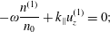 $$\begin{eqnarray}\displaystyle & \displaystyle -\unicode[STIX]{x1D714}\frac{n^{(1)}}{n_{0}}+k_{\Vert }u_{z}^{(1)}=0; & \displaystyle\end{eqnarray}$$
 $$\begin{eqnarray}\displaystyle & \displaystyle -\unicode[STIX]{x1D714}u_{z}^{(1)}+\frac{v_{\text{th}\Vert }^{2}}{2}k_{\Vert }\frac{p_{\Vert }^{(1)}}{p_{\Vert }^{(0)}}=0; & \displaystyle\end{eqnarray}$$
 $$\begin{eqnarray}\displaystyle & \displaystyle -\unicode[STIX]{x1D714}\frac{p_{\Vert }^{(1)}}{p_{\Vert }^{(0)}}+3k_{\Vert }u_{z}^{(1)}+k_{\Vert }\frac{q_{\Vert }^{(1)}}{p_{\Vert }^{(0)}}=0; & \displaystyle\end{eqnarray}$$
 $$\begin{eqnarray}\displaystyle & \displaystyle -\unicode[STIX]{x1D714}\frac{q_{\Vert }^{(1)}}{p_{\Vert }^{(0)}}+\frac{3}{2}v_{\text{th}\Vert }^{2}k_{\Vert }\left(\frac{p_{\Vert }^{(1)}}{p_{\Vert }^{(0)}}-\frac{n^{(1)}}{n_{0}}\right)+k_{\Vert }\frac{\widetilde{r}_{\Vert \Vert }^{(1)}}{p_{\Vert }^{(0)}}=0, & \displaystyle\end{eqnarray}$$
where the fluctuating parallel temperature
 $T_{\Vert }^{(1)}$
is linearized as
$T_{\Vert }^{(1)}$
is linearized as
 $$\begin{eqnarray}\frac{T_{\Vert }^{(1)}}{T_{\Vert }^{(0)}}=\frac{p_{\Vert }^{(1)}}{p_{\Vert }^{(0)}}-\frac{n^{(1)}}{n_{0}}.\end{eqnarray}$$
The superscript (1) on quantities
 $n^{(1)}$
,
$n^{(1)}$
,
 $u_{z}^{(1)}$
,
$u_{z}^{(1)}$
,
 $p_{\Vert }^{(1)}$
,
$p_{\Vert }^{(1)}$
,
 $q_{\Vert }^{(1)}$
(and
$q_{\Vert }^{(1)}$
(and
 $T_{\Vert }^{(1)}$
) signifies that these are just fluctuating quantities, the superscript does not mean here that these quantities are obtained by integration over the kinetic
$T_{\Vert }^{(1)}$
) signifies that these are just fluctuating quantities, the superscript does not mean here that these quantities are obtained by integration over the kinetic
 $f^{(1)}$
. This fluid model is accompanied by a closure for
$f^{(1)}$
. This fluid model is accompanied by a closure for
 $\widetilde{r}_{\Vert \Vert }^{(1)}$
, and that one was obtained from linear kinetic theory by integrating over the kinetic
$\widetilde{r}_{\Vert \Vert }^{(1)}$
, and that one was obtained from linear kinetic theory by integrating over the kinetic
 $f^{(1)}$
. Let us choose the
$f^{(1)}$
. Let us choose the
 $R_{4,3}(\unicode[STIX]{x1D701})$
closure, equation (3.234)
$R_{4,3}(\unicode[STIX]{x1D701})$
closure, equation (3.234)
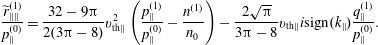 $$\begin{eqnarray}\frac{\widetilde{r}_{\Vert \Vert }^{(1)}}{p_{\Vert }^{(0)}}=\frac{32-9\unicode[STIX]{x03C0}}{2(3\unicode[STIX]{x03C0}-8)}v_{\text{th}\Vert }^{2}\left(\frac{p_{\Vert }^{(1)}}{p_{\Vert }^{(0)}}-\frac{n^{(1)}}{n_{0}}\right)-\frac{2\sqrt{\unicode[STIX]{x03C0}}}{3\unicode[STIX]{x03C0}-8}v_{\text{th}\Vert }i\text{sign}(k_{\Vert })\frac{q_{\Vert }^{(1)}}{p_{\Vert }^{(0)}}.\end{eqnarray}$$
Now the model is closed, and calculating the determinant yields the following dispersion relation
 $$\begin{eqnarray}\displaystyle & & \displaystyle \unicode[STIX]{x1D714}^{4}+\frac{2i\sqrt{\unicode[STIX]{x03C0}}}{3\unicode[STIX]{x03C0}-8}k_{\Vert }v_{\text{th}\Vert }\text{sign}(k_{\Vert })\unicode[STIX]{x1D714}^{3}-\frac{(9\unicode[STIX]{x03C0}-16)}{2(3\unicode[STIX]{x03C0}-8)}k_{\Vert }^{2}v_{\text{th}\Vert }^{2}\unicode[STIX]{x1D714}^{2}\nonumber\\ \displaystyle & & \displaystyle \qquad -\,\frac{3i\sqrt{\unicode[STIX]{x03C0}}}{3\unicode[STIX]{x03C0}-8}k_{\Vert }^{3}v_{\text{th}\Vert }^{3}\text{sign}(k_{\Vert })\unicode[STIX]{x1D714}+\frac{2}{3\unicode[STIX]{x03C0}-8}k_{\Vert }^{4}v_{\text{th}\Vert }^{4}=0.\end{eqnarray}$$
By examining the expression, an obvious substitution offers itself
 $$\begin{eqnarray}\unicode[STIX]{x1D701}=\frac{\unicode[STIX]{x1D714}}{\text{sign}(k_{\Vert })k_{\Vert }v_{\text{th}\Vert }}=\frac{\unicode[STIX]{x1D714}}{|k_{\Vert }|v_{\text{th}\Vert }},\end{eqnarray}$$
that transforms the polynomial to a completely dimensionless form
 $$\begin{eqnarray}\unicode[STIX]{x1D701}^{4}+\frac{2i\sqrt{\unicode[STIX]{x03C0}}}{3\unicode[STIX]{x03C0}-8}\unicode[STIX]{x1D701}^{3}-\frac{9\unicode[STIX]{x03C0}-16}{2(3\unicode[STIX]{x03C0}-8)}\unicode[STIX]{x1D701}^{2}-\frac{3i\sqrt{\unicode[STIX]{x03C0}}}{3\unicode[STIX]{x03C0}-8}\unicode[STIX]{x1D701}+\frac{2}{3\unicode[STIX]{x03C0}-8}=0.\end{eqnarray}$$
The
 $\unicode[STIX]{x1D701}$
is obviously a very useful quantity, and one could rewrite the fluid equations (3.340)–(3.343) directly with this quantity. The polynomial (3.348) can be solved numerically, and the approximate solutions are (writing only 3 decimal digits)
$\unicode[STIX]{x1D701}$
is obviously a very useful quantity, and one could rewrite the fluid equations (3.340)–(3.343) directly with this quantity. The polynomial (3.348) can be solved numerically, and the approximate solutions are (writing only 3 decimal digits)
 $$\begin{eqnarray}\unicode[STIX]{x1D701}=\pm 1.359-0.534i;\quad \unicode[STIX]{x1D701}=\pm 0.392-0.710i,\end{eqnarray}$$
yielding solutions in physical units
 $$\begin{eqnarray}\displaystyle \unicode[STIX]{x1D714}=|k_{\Vert }|v_{\text{th}\Vert }(\pm 1.359-0.534i);\quad \unicode[STIX]{x1D714}=|k_{\Vert }|v_{\text{th}\Vert }(\pm 0.392-0.710i). & & \displaystyle\end{eqnarray}$$
The first solution is the ion-acoustic (sound) mode and the second solution is ‘a higher-order mode’. Both solutions are highly damped, and the higher-order mode has actually a higher damping rate than its real frequency. We can now also see how important was to keep track of the
 $\text{sign}(k_{\Vert })$
, since the modes are damped for both
$\text{sign}(k_{\Vert })$
, since the modes are damped for both
 $k_{\Vert }>0$
and
$k_{\Vert }>0$
and
 $k_{\Vert }<0$
. If we had ignored the
$k_{\Vert }<0$
. If we had ignored the
 $\text{sign}(k_{\Vert })$
, we would obtain that, for
$\text{sign}(k_{\Vert })$
, we would obtain that, for
 $k_{\Vert }<0$
, the sound mode has a positive growth rate and is unstable, which would be unphysical.
$k_{\Vert }<0$
, the sound mode has a positive growth rate and is unstable, which would be unphysical.
Of course, each closure will yield a different dispersion relation. Exploring the simplest closure with quasi-static heat flux
 $q_{\Vert }^{(1)}$
obtained with
$q_{\Vert }^{(1)}$
obtained with
 $R_{3,2}(\unicode[STIX]{x1D701})$
, equations (3.340)–(3.342) are closed by
$R_{3,2}(\unicode[STIX]{x1D701})$
, equations (3.340)–(3.342) are closed by
 $$\begin{eqnarray}\frac{q_{\Vert }^{(1)}}{p_{\Vert }^{(0)}}=-\frac{2}{\sqrt{\unicode[STIX]{x03C0}}}v_{\text{th}\Vert }i\text{sign}(k_{\Vert })\left(\frac{p_{\Vert }^{(1)}}{p_{\Vert }^{(0)}}-\frac{n^{(1)}}{n_{0}}\right),\end{eqnarray}$$
which yields a polynomial
 $$\begin{eqnarray}\unicode[STIX]{x1D701}^{3}+\frac{2i}{\sqrt{\unicode[STIX]{x03C0}}}\unicode[STIX]{x1D701}^{2}-\frac{3}{2}\unicode[STIX]{x1D701}-\frac{i}{\sqrt{\unicode[STIX]{x03C0}}}=0.\end{eqnarray}$$
Numerical solutions are
 $\unicode[STIX]{x1D701}=\pm 1.041-0.327i$
;
$\unicode[STIX]{x1D701}=\pm 1.041-0.327i$
;
 $\unicode[STIX]{x1D701}=-0.474i$
, showing that, in this case, the higher-order mode does not propagate and is purely damped. The ion-acoustic mode is also very damped and has a dispersion relation
$\unicode[STIX]{x1D701}=-0.474i$
, showing that, in this case, the higher-order mode does not propagate and is purely damped. The ion-acoustic mode is also very damped and has a dispersion relation
 $$\begin{eqnarray}\displaystyle \unicode[STIX]{x1D714}=|k_{\Vert }|v_{\text{th}\Vert }(\pm 1.041-0.327i). & & \displaystyle\end{eqnarray}$$
We examine two more closures. The most precise quasi-static closure (3.227) obtained with
 $R_{4,2}(\unicode[STIX]{x1D701})$
yields the analytic dispersion relation
$R_{4,2}(\unicode[STIX]{x1D701})$
yields the analytic dispersion relation
 $$\begin{eqnarray}\unicode[STIX]{x1D701}^{4}+i\sqrt{\unicode[STIX]{x03C0}}\frac{10-3\unicode[STIX]{x03C0}}{16-5\unicode[STIX]{x03C0}}\unicode[STIX]{x1D701}^{3}-\frac{32-9\unicode[STIX]{x03C0}}{32-10\unicode[STIX]{x03C0}}\unicode[STIX]{x1D701}^{2}-\frac{i\sqrt{\unicode[STIX]{x03C0}}}{16-5\unicode[STIX]{x03C0}}\unicode[STIX]{x1D701}+\frac{3\unicode[STIX]{x03C0}-8}{32-10\unicode[STIX]{x03C0}}=0,\end{eqnarray}$$
and the solutions are
 $$\begin{eqnarray}\displaystyle \unicode[STIX]{x1D714}=|k_{\Vert }|v_{\text{th}\Vert }(\pm 1.294-0.790i);\quad \unicode[STIX]{x1D714}=|k_{\Vert }|v_{\text{th}\Vert }(\pm 0.385-0.956i), & & \displaystyle\end{eqnarray}$$
the first one being the ion-acoustic mode. Finally, the only available
 $o(\unicode[STIX]{x1D701}^{4})$
closure (3.339) obtained with
$o(\unicode[STIX]{x1D701}^{4})$
closure (3.339) obtained with
 $R_{5,3}(\unicode[STIX]{x1D701})$
yields the analytic dispersion relation
$R_{5,3}(\unicode[STIX]{x1D701})$
yields the analytic dispersion relation
 $$\begin{eqnarray}\unicode[STIX]{x1D701}^{5}+i\widetilde{\unicode[STIX]{x1D6FC}}_{r}\unicode[STIX]{x1D701}^{4}+(\widetilde{\unicode[STIX]{x1D6FC}}_{q}-3)\unicode[STIX]{x1D701}^{3}-i(3\widetilde{\unicode[STIX]{x1D6FC}}_{r}-\widetilde{\unicode[STIX]{x1D6FC}}_{T})\unicode[STIX]{x1D701}^{2}+\frac{1}{2}\left(\widetilde{\unicode[STIX]{x1D6FC}}_{u}-3\widetilde{\unicode[STIX]{x1D6FC}}_{q}+\frac{3}{2}\right)\unicode[STIX]{x1D701}+\frac{i}{4}(3\widetilde{\unicode[STIX]{x1D6FC}}_{r}-2\widetilde{\unicode[STIX]{x1D6FC}}_{T})=0,\end{eqnarray}$$
where the coefficients are specified in (3.335), and the numerical solutions are
 $$\begin{eqnarray}\unicode[STIX]{x1D714}=|k_{\Vert }|v_{\text{th}\Vert }(\pm 1.589-0.908i);\quad \unicode[STIX]{x1D714}=|k_{\Vert }|v_{\text{th}\Vert }(\pm 0.710-1.084i);\quad \unicode[STIX]{x1D714}=|k_{\Vert }|v_{\text{th}\Vert }(-1.147i),\end{eqnarray}$$
the first being the ion-acoustic mode.
Let us compare the obtained results. Perhaps curiously, it appears that, as the precision of closures increases, so does i the real frequency and the damping rate of the ion-acoustic mode, and the differences are quite significant. So what is the correct kinetic result, i.e. how close did we get to the kinetic theory? That is not as easy a question as it appears to be. By opening kinetic books, there is no such discussion on the long-wavelength limit of the ion-acoustic mode, when the electrons are cold. Even the exact numerical solutions are usually considered only for
 $T_{e}/T_{p}\geqslant 1$
, see for example figure 9.18 on page 355 in Gurnett and Bhattacharjee.
$T_{e}/T_{p}\geqslant 1$
, see for example figure 9.18 on page 355 in Gurnett and Bhattacharjee.
Let us examine the analytic dispersion relations (3.348), (3.352), (3.354) and (3.356), that were obtained with approximants
 $R_{4,3}(\unicode[STIX]{x1D701})$
,
$R_{4,3}(\unicode[STIX]{x1D701})$
,
 $R_{3,2}(\unicode[STIX]{x1D701})$
,
$R_{3,2}(\unicode[STIX]{x1D701})$
,
 $R_{4,2}(\unicode[STIX]{x1D701})$
and
$R_{4,2}(\unicode[STIX]{x1D701})$
and
 $R_{5,3}(\unicode[STIX]{x1D701})$
. One notices that the dispersion relations exactly match the denominators of the associated Padé approximants! Or in another words, without doing any calculations whatsoever, it appears that if a closure of a 1-D fluid model is available for a
$R_{5,3}(\unicode[STIX]{x1D701})$
. One notices that the dispersion relations exactly match the denominators of the associated Padé approximants! Or in another words, without doing any calculations whatsoever, it appears that if a closure of a 1-D fluid model is available for a
 $R_{n,n^{\prime }}(\unicode[STIX]{x1D701})$
approximant, the dispersion relation is equivalent to the denominator of that
$R_{n,n^{\prime }}(\unicode[STIX]{x1D701})$
approximant, the dispersion relation is equivalent to the denominator of that
 $R_{n,n^{\prime }}(\unicode[STIX]{x1D701})$
. How is this possible? The explanation is simple if one considers the electrostatic kinetic dispersion relation for the proton and electron species (3.30), which at scales that are much longer than the Debye length simplifies to (3.366). Prescribing massless electrons yields
$R_{n,n^{\prime }}(\unicode[STIX]{x1D701})$
. How is this possible? The explanation is simple if one considers the electrostatic kinetic dispersion relation for the proton and electron species (3.30), which at scales that are much longer than the Debye length simplifies to (3.366). Prescribing massless electrons yields
 $R(\unicode[STIX]{x1D701}_{e})=1$
, implying dispersion relation
$R(\unicode[STIX]{x1D701}_{e})=1$
, implying dispersion relation
 $R(\unicode[STIX]{x1D701}_{p})=-T_{p}^{(0)}/T_{e}^{(0)}$
. For cold electrons, both real and imaginary parts of
$R(\unicode[STIX]{x1D701}_{p})=-T_{p}^{(0)}/T_{e}^{(0)}$
. For cold electrons, both real and imaginary parts of
 $R(\unicode[STIX]{x1D701}_{p})$
obviously diverge, so that
$R(\unicode[STIX]{x1D701}_{p})$
obviously diverge, so that
 $$\begin{eqnarray}\frac{1}{R(\unicode[STIX]{x1D701}_{p})}=0.\end{eqnarray}$$
The above expression can be considered the electrostatic dispersion relation of a proton–electron plasma, where the electrons are massless and completely cold. The reason why such an expression cannot be found in any plasma book is that, from the kinetic perspective, such an expression cannot be solved and is ill defined. The function
 $R(\unicode[STIX]{x1D701})$
is directly related to the derivative of
$R(\unicode[STIX]{x1D701})$
is directly related to the derivative of
 $Z(\unicode[STIX]{x1D701})$
according to
$Z(\unicode[STIX]{x1D701})$
according to
 $Z^{\prime }(\unicode[STIX]{x1D701})=-2R(\unicode[STIX]{x1D701})$
. Infinitely large
$Z^{\prime }(\unicode[STIX]{x1D701})=-2R(\unicode[STIX]{x1D701})$
. Infinitely large
 $R(\unicode[STIX]{x1D701})$
means that
$R(\unicode[STIX]{x1D701})$
means that
 $Z(\unicode[STIX]{x1D701})$
has infinitely large derivatives, i.e. that
$Z(\unicode[STIX]{x1D701})$
has infinitely large derivatives, i.e. that
 $Z(\unicode[STIX]{x1D701})$
is not continuous and not analytic, which contradicts the entire definition of
$Z(\unicode[STIX]{x1D701})$
is not continuous and not analytic, which contradicts the entire definition of
 $Z(\unicode[STIX]{x1D701})$
and how the function was constructed. However, when Padé approximants of these functions are considered, and when
$Z(\unicode[STIX]{x1D701})$
and how the function was constructed. However, when Padé approximants of these functions are considered, and when
 $R(\unicode[STIX]{x1D701})$
is replaced by
$R(\unicode[STIX]{x1D701})$
is replaced by
 $R_{n,n^{\prime }}(\unicode[STIX]{x1D701})$
, so that
$R_{n,n^{\prime }}(\unicode[STIX]{x1D701})$
, so that
such an expression does make sense, and is equivalent to the denominator of
 $R_{n,n^{\prime }}(\unicode[STIX]{x1D701})$
being zero, i.e. it directly yields the dispersion relations of the considered fluid models. We note that while the plasma dispersion function corresponding to a Maxwellian distribution function does not display singularities at finite distance in the complex plane, this is not the case when considering kappa distribution functions, see e.g. Podesta (Reference Podesta2004).
$R_{n,n^{\prime }}(\unicode[STIX]{x1D701})$
being zero, i.e. it directly yields the dispersion relations of the considered fluid models. We note that while the plasma dispersion function corresponding to a Maxwellian distribution function does not display singularities at finite distance in the complex plane, this is not the case when considering kappa distribution functions, see e.g. Podesta (Reference Podesta2004).
3.12.1 The proton Landau damping does not disappear at long wavelengths
There are several extremely interesting phenomena worth discussing. (i) In the dispersion relation for the ion-acoustic (sound) mode (3.350), the usual phase speed
 $\unicode[STIX]{x1D714}/k_{\Vert }$
is constant, implying that the Landau damping (of the parallel propagating sound mode) does not disappear, however long wavelengths are considered. With cold electrons, as considered here, the parallel sound mode is always heavily damped, and disappears in a few wavelengths, even on large astrophysical scales. A very good discussion can be found for example in Howes (Reference Howes2009), who concluded that, in general (unless electrons are hot), the MHD sound mode represents an unphysical spurious wave that does not exist in collisionless plasma. (ii) The equations (3.340)–(3.343) do not even contain the parallel electric field
$\unicode[STIX]{x1D714}/k_{\Vert }$
is constant, implying that the Landau damping (of the parallel propagating sound mode) does not disappear, however long wavelengths are considered. With cold electrons, as considered here, the parallel sound mode is always heavily damped, and disappears in a few wavelengths, even on large astrophysical scales. A very good discussion can be found for example in Howes (Reference Howes2009), who concluded that, in general (unless electrons are hot), the MHD sound mode represents an unphysical spurious wave that does not exist in collisionless plasma. (ii) The equations (3.340)–(3.343) do not even contain the parallel electric field
 $E_{\Vert }$
. This might sound surprising, but the parallel electric field completely disappears at long wavelengths, even though the Landau damping (as expressed through the constant phase speed), does not disappear. The parallel electric field does not disappear, if electrons have finite temperature, it also enters (very weakly), if the electron inertia is included. In the 1-D linearized geometry considered here, the contributions will be
$E_{\Vert }$
. This might sound surprising, but the parallel electric field completely disappears at long wavelengths, even though the Landau damping (as expressed through the constant phase speed), does not disappear. The parallel electric field does not disappear, if electrons have finite temperature, it also enters (very weakly), if the electron inertia is included. In the 1-D linearized geometry considered here, the contributions will be
 $$\begin{eqnarray}E_{\Vert }=-\frac{1}{en_{0}}\unicode[STIX]{x2202}_{z}p_{\Vert e}-\frac{m_{e}}{e}\frac{\unicode[STIX]{x2202}u_{ze}}{\unicode[STIX]{x2202}t}.\end{eqnarray}$$
(iii) The presence of Landau damping in the long-wavelength limit is exactly the reason why usual fluid models such as MHD, or even the much more sophisticated CGL description, do not converge to the collisionless kinetic theory, whatever long wavelengths and low frequencies are considered. There is always a mismatch in dispersion relations when the phase speed is plotted that, depending on plasma parameters, can be quite large. This does not concern only the damping rate (which in MHD and CGL is of course zero), the differences in the real frequency, which is always coupled to the imaginary frequency (for example through the polynomial (3.348) for that specific closure), can be large too. (iv) If the heat flux
 $q_{\Vert }^{(1)}$
is prescribed to be zero, i.e. if a CGL model is prescribed, the dispersion relation of the parallel propagating sound mode is determined only by the parallel velocity equation (3.341) and parallel pressure equation (3.342), yielding the CGL result
$q_{\Vert }^{(1)}$
is prescribed to be zero, i.e. if a CGL model is prescribed, the dispersion relation of the parallel propagating sound mode is determined only by the parallel velocity equation (3.341) and parallel pressure equation (3.342), yielding the CGL result
 $\unicode[STIX]{x1D714}^{2}=\frac{3}{2}v_{\text{th}\Vert }^{2}k_{\Vert }^{2}$
, so that
$\unicode[STIX]{x1D714}^{2}=\frac{3}{2}v_{\text{th}\Vert }^{2}k_{\Vert }^{2}$
, so that
 $$\begin{eqnarray}\unicode[STIX]{x1D714}^{\text{CGL}}=\pm |k_{\Vert }|v_{\text{th}\Vert }\sqrt{{\textstyle \frac{3}{2}}}=\pm |k_{\Vert }|v_{\text{th}\Vert }1.225.\end{eqnarray}$$
For comparison, the MHD result can be written with the usual MHD sound speed
 $C_{s}^{2}=\unicode[STIX]{x1D6FE}(p_{0}/\unicode[STIX]{x1D70C}_{0})=(\unicode[STIX]{x1D6FE}/2)v_{\text{th}}^{2}$
where
$C_{s}^{2}=\unicode[STIX]{x1D6FE}(p_{0}/\unicode[STIX]{x1D70C}_{0})=(\unicode[STIX]{x1D6FE}/2)v_{\text{th}}^{2}$
where
 $\unicode[STIX]{x1D6FE}=5/3$
, so
$\unicode[STIX]{x1D6FE}=5/3$
, so
 $$\begin{eqnarray}\unicode[STIX]{x1D714}^{\text{MHD}}=\pm |k_{\Vert }|v_{\text{th}}\sqrt{{\textstyle \frac{5}{6}}}=\pm |k_{\Vert }|v_{\text{th}}0.913.\end{eqnarray}$$
It is important to examine the influence of isothermal electron species.
3.13 Proton Landau damping, influence of isothermal electrons
Let us prescribe electrons to be isothermal, with some finite electron temperature, but let us neglect the electron inertia. The proton momentum equation is changed to (3.372), the electron pressure equation reads
 $$\begin{eqnarray}-\unicode[STIX]{x1D714}\frac{p_{\Vert e}^{(1)}}{p_{\Vert p}^{(0)}}+k_{\Vert }\unicode[STIX]{x1D70F}u_{z}^{(1)}=0;\quad \unicode[STIX]{x1D70F}\equiv \frac{T_{\Vert e}^{(0)}}{T_{\Vert p}^{(0)}},\end{eqnarray}$$
where for brevity, we define the ratio of electron and proton temperature as
 $\unicode[STIX]{x1D70F}$
. Using the
$\unicode[STIX]{x1D70F}$
. Using the
 $R_{4,3}(\unicode[STIX]{x1D701})$
closure as before, the coupled dispersion relation reads
$R_{4,3}(\unicode[STIX]{x1D701})$
closure as before, the coupled dispersion relation reads
 $$\begin{eqnarray}\unicode[STIX]{x1D701}^{4}+\frac{2i\sqrt{\unicode[STIX]{x03C0}}}{3\unicode[STIX]{x03C0}-8}\unicode[STIX]{x1D701}^{3}-\frac{9\unicode[STIX]{x03C0}-16+(3\unicode[STIX]{x03C0}-8)\unicode[STIX]{x1D70F}}{2(3\unicode[STIX]{x03C0}-8)}\unicode[STIX]{x1D701}^{2}-\frac{i\sqrt{\unicode[STIX]{x03C0}}(3+\unicode[STIX]{x1D70F})}{3\unicode[STIX]{x03C0}-8}\unicode[STIX]{x1D701}+\frac{2(1+\unicode[STIX]{x1D70F})}{3\unicode[STIX]{x03C0}-8}=0.\end{eqnarray}$$
The above expression is equivalent to (A6) in Hunana et al. (Reference Hunana, Laveder, Passot, Sulem and Borgogno2011).Footnote
9
The
 $R_{4,2}(\unicode[STIX]{x1D701})$
closure yields dispersion relation
$R_{4,2}(\unicode[STIX]{x1D701})$
closure yields dispersion relation
 $$\begin{eqnarray}\displaystyle & & \displaystyle \unicode[STIX]{x1D701}^{4}+\frac{i\sqrt{\unicode[STIX]{x03C0}}(10-3\unicode[STIX]{x03C0})}{16-5\unicode[STIX]{x03C0}}\unicode[STIX]{x1D701}^{3}-\frac{32-9\unicode[STIX]{x03C0}+(16-5\unicode[STIX]{x03C0})\unicode[STIX]{x1D70F}}{32-10\unicode[STIX]{x03C0}}\unicode[STIX]{x1D701}^{2}\nonumber\\ \displaystyle & & \displaystyle \qquad -\,\frac{i\sqrt{\unicode[STIX]{x03C0}}(2+(10-3\unicode[STIX]{x03C0})\unicode[STIX]{x1D70F})}{32-10\unicode[STIX]{x03C0}}\unicode[STIX]{x1D701}+\frac{(3\unicode[STIX]{x03C0}-8)(1+\unicode[STIX]{x1D70F})}{32-10\unicode[STIX]{x03C0}}=0.\end{eqnarray}$$
Let us use (3.363) and focus on the ion-acoustic mode, since the higher-order mode is always highly damped. Solutions for a few different
 $\unicode[STIX]{x1D70F}$
values are
$\unicode[STIX]{x1D70F}$
values are
 $$\begin{eqnarray}\displaystyle \unicode[STIX]{x1D70F}=0:\quad \unicode[STIX]{x1D701} & = & \displaystyle \pm 1.359-0.534i;\nonumber\\ \displaystyle \unicode[STIX]{x1D70F}=0.1:\quad \unicode[STIX]{x1D701} & = & \displaystyle \pm 1.367-0.514i;\nonumber\\ \displaystyle \unicode[STIX]{x1D70F}=0.5:\quad \unicode[STIX]{x1D701} & = & \displaystyle \pm 1.409-0.439i;\nonumber\\ \displaystyle \unicode[STIX]{x1D70F}=1.0:\quad \unicode[STIX]{x1D701} & = & \displaystyle \pm 1.481-0.361i;\nonumber\\ \displaystyle \unicode[STIX]{x1D70F}=2.0:\quad \unicode[STIX]{x1D701} & = & \displaystyle \pm 1.640-0.260i;\nonumber\\ \displaystyle \unicode[STIX]{x1D70F}=5.0:\quad \unicode[STIX]{x1D701} & = & \displaystyle \pm 2.054-0.131i;\nonumber\\ \displaystyle \unicode[STIX]{x1D70F}=10.0:\quad \unicode[STIX]{x1D701} & = & \displaystyle \pm 2.591-0.061i;\nonumber\\ \displaystyle \unicode[STIX]{x1D70F}=100.0:\quad \unicode[STIX]{x1D701} & = & \displaystyle \pm 7.180-0.001i.\end{eqnarray}$$
This is excellent, as in kinetic books, with increasing electron temperature, the Landau damping of the ion-acoustic mode decreases. Compared to kinetic calculations (see the last column in (3.381)), the total Landau damping is here of course underestimated, especially for high electron temperatures, since here in the fluid model, only the proton Landau damping is contributing, and the electron Landau damping is turned off. Let us turn it on.
3.14 Proton and electron Landau damping
Considering wavelengths much longer than the Debye length, the exact kinetic dispersion relation reads

where the electron thermal velocity
 $$\begin{eqnarray}v_{\text{th}\Vert e}=v_{\text{th}\Vert p}\sqrt{\frac{m_{p}}{m_{e}}}\sqrt{\frac{T_{\Vert e}^{(0)}}{T_{\Vert p}^{(0)}}},\end{eqnarray}$$
is of course much higher than the proton thermal velocity (unless the electrons are cold), and by using the abbreviated
 $$\begin{eqnarray}\unicode[STIX]{x1D70F}\equiv \frac{T_{\Vert e}^{(0)}}{T_{\Vert p}^{(0)}};\quad \unicode[STIX]{x1D707}\equiv \frac{m_{e}}{m_{p}},\end{eqnarray}$$
so that
 $$\begin{eqnarray}\unicode[STIX]{x1D701}_{p}=\frac{\unicode[STIX]{x1D714}}{|k_{\Vert }|v_{\text{th}\Vert p}};\quad \unicode[STIX]{x1D701}_{e}=\frac{\unicode[STIX]{x1D714}}{|k_{\Vert }|v_{\text{th}\Vert e}}=\unicode[STIX]{x1D701}_{p}\sqrt{\frac{\unicode[STIX]{x1D707}}{\unicode[STIX]{x1D70F}}},\end{eqnarray}$$
and the exact kinetic dispersion relation reads
 $$\begin{eqnarray}\unicode[STIX]{x1D70F}R(\unicode[STIX]{x1D701}_{p})+R\left(\unicode[STIX]{x1D701}_{p}\sqrt{\unicode[STIX]{x1D707}/\unicode[STIX]{x1D70F}}\right)=0.\end{eqnarray}$$
Let us see how close we got. One of the greatest advantages of Landau fluid models is that we do not have to resolve electron motion to obtain the correct form of electron Landau damping at long wavelengths, and the electron inertia in the electron momentum equation can be neglected. The correct electron–proton mass ratio can enter equations for the electron heat flux
 $q_{\Vert e}$
and the fourth-order moment
$q_{\Vert e}$
and the fourth-order moment
 $\widetilde{r}_{\Vert \Vert e}$
, and the electron inertia influences the solutions only insignificantly. However, let us keep the electron inertia for a moment. The equations for the proton species read
$\widetilde{r}_{\Vert \Vert e}$
, and the electron inertia influences the solutions only insignificantly. However, let us keep the electron inertia for a moment. The equations for the proton species read
 $$\begin{eqnarray}\displaystyle & \displaystyle -\unicode[STIX]{x1D714}\frac{n^{(1)}}{n_{0}}+k_{\Vert }u_{z}^{(1)}=0; & \displaystyle\end{eqnarray}$$
 $$\begin{eqnarray}\displaystyle & \displaystyle -\unicode[STIX]{x1D714}u_{z}^{(1)}+\frac{v_{\text{th}\Vert p}^{2}}{2}k_{\Vert }\left(\frac{p_{\Vert p}^{(1)}}{p_{\Vert p}^{(0)}}+\frac{p_{\Vert e}^{(1)}}{p_{\Vert p}^{(0)}}\right)-\unicode[STIX]{x1D714}\frac{m_{e}}{m_{p}}u_{z}^{(1)}=0; & \displaystyle\end{eqnarray}$$
 $$\begin{eqnarray}\displaystyle & \displaystyle -\unicode[STIX]{x1D714}\frac{p_{\Vert p}^{(1)}}{p_{\Vert p}^{(0)}}+3k_{\Vert }u_{z}^{(1)}+k_{\Vert }\frac{q_{\Vert p}^{(1)}}{p_{\Vert p}^{(0)}}=0; & \displaystyle\end{eqnarray}$$
 $$\begin{eqnarray}\displaystyle & \displaystyle -\unicode[STIX]{x1D714}\frac{q_{\Vert p}^{(1)}}{p_{\Vert p}^{(0)}}+\frac{3}{2}v_{\text{th}\Vert p}^{2}k_{\Vert }\left(\frac{p_{\Vert p}^{(1)}}{p_{\Vert p}^{(0)}}-\frac{n^{(1)}}{n_{0}}\right)+k_{\Vert }\frac{\widetilde{r}_{\Vert \Vert p}^{(1)}}{p_{\Vert p}^{(0)}}=0, & \displaystyle\end{eqnarray}$$
and the electron inertia represents the last term in (3.372). The electron equations are written in a form so that they are normalized with respect to the proton pressure
 $$\begin{eqnarray}\displaystyle & \displaystyle -\unicode[STIX]{x1D714}\frac{p_{\Vert e}^{(1)}}{p_{\Vert p}^{(0)}}+3k_{\Vert }\unicode[STIX]{x1D70F}u_{z}^{(1)}+k_{\Vert }\frac{q_{\Vert e}^{(1)}}{p_{\Vert p}^{(0)}}=0; & \displaystyle\end{eqnarray}$$
 $$\begin{eqnarray}\displaystyle & \displaystyle -\unicode[STIX]{x1D714}\frac{q_{\Vert e}^{(1)}}{p_{\Vert p}^{(0)}}+\frac{3}{2}v_{\text{th}\Vert p}^{2}\frac{m_{p}}{m_{e}}k_{\Vert }\unicode[STIX]{x1D70F}\left(\frac{p_{\Vert e}^{(1)}}{p_{\Vert p}^{(0)}}-\unicode[STIX]{x1D70F}\frac{n^{(1)}}{n_{0}}\right)+k_{\Vert }\frac{\widetilde{r}_{\Vert \Vert e}^{(1)}}{p_{\Vert p}^{(0)}}=0. & \displaystyle\end{eqnarray}$$
Note that the electron fluid speed
 $u_{ze}^{(1)}=u_{zp}^{(1)}$
(so we omitted the index
$u_{ze}^{(1)}=u_{zp}^{(1)}$
(so we omitted the index
 $p$
). The fluid equations are accompanied by a closure from kinetic theory, for example the
$p$
). The fluid equations are accompanied by a closure from kinetic theory, for example the
 $R_{4,3}(\unicode[STIX]{x1D701})$
closure
$R_{4,3}(\unicode[STIX]{x1D701})$
closure
 $$\begin{eqnarray}\displaystyle & \displaystyle \frac{\widetilde{r}_{\Vert \Vert p}^{(1)}}{p_{\Vert p}^{(0)}}=\frac{32-9\unicode[STIX]{x03C0}}{2(3\unicode[STIX]{x03C0}-8)}v_{\text{th}\Vert p}^{2}\left(\frac{p_{\Vert p}^{(1)}}{p_{\Vert p}^{(0)}}-\frac{n^{(1)}}{n_{0}}\right)-\frac{2\sqrt{\unicode[STIX]{x03C0}}}{3\unicode[STIX]{x03C0}-8}v_{\text{th}\Vert p}i\text{sign}(k_{\Vert })\frac{q_{\Vert p}^{(1)}}{p_{\Vert p}^{(0)}}, & \displaystyle\end{eqnarray}$$
 $$\begin{eqnarray}\displaystyle & \displaystyle \frac{\widetilde{r}_{\Vert \Vert e}^{(1)}}{p_{\Vert p}^{(0)}}=\frac{32-9\unicode[STIX]{x03C0}}{2(3\unicode[STIX]{x03C0}-8)}v_{\text{th}\Vert p}^{2}\frac{m_{p}}{m_{e}}\unicode[STIX]{x1D70F}\left(\frac{p_{\Vert e}^{(1)}}{p_{\Vert p}^{(0)}}-\unicode[STIX]{x1D70F}\frac{n^{(1)}}{n_{0}}\right)-\frac{2\sqrt{\unicode[STIX]{x03C0}}}{3\unicode[STIX]{x03C0}-8}v_{\text{th}\Vert p}\sqrt{\frac{m_{p}}{m_{e}}}\sqrt{\unicode[STIX]{x1D70F}}i\text{sign}(k_{\Vert })\frac{q_{\Vert e}^{(1)}}{p_{\Vert p}^{(0)}}. & \displaystyle \nonumber\\ \displaystyle & & \displaystyle\end{eqnarray}$$
The equations (3.371)–(3.378) now represents a fluid description of the ion-acoustic mode, and contain both proton and electron Landau damping. It is rather mesmerizing that the relatively complicated dispersion relation of this fluid model can be shown to be equivalent to the ‘simple looking’ kinetic dispersion relation
 $$\begin{eqnarray}\unicode[STIX]{x1D70F}R_{4,3}(\unicode[STIX]{x1D701}_{p})+R_{4,3}\left(\unicode[STIX]{x1D701}_{p}\sqrt{\unicode[STIX]{x1D707}/\unicode[STIX]{x1D70F}}\right)=0,\end{eqnarray}$$
i.e. equivalent to the full kinetic dispersion relation (3.370), where the exact
 $R(\unicode[STIX]{x1D701})$
is replaced with the
$R(\unicode[STIX]{x1D701})$
is replaced with the
 $R_{4,3}(\unicode[STIX]{x1D701})$
approximant (by transferring the proton and electron terms of
$R_{4,3}(\unicode[STIX]{x1D701})$
approximant (by transferring the proton and electron terms of
 $R_{4,3}(\unicode[STIX]{x1D701})$
in the expression (3.379) to the common denominator and making the resulting numerator of that expression equal to zero, Maple is great in this regard).
$R_{4,3}(\unicode[STIX]{x1D701})$
in the expression (3.379) to the common denominator and making the resulting numerator of that expression equal to zero, Maple is great in this regard).
Nevertheless, here, we want clearly demonstrate that the electron inertia can be neglected and the electron Landau damping still nicely captured, and we use fluid dispersion relations obtained from the system (3.371)–(3.378), where the last term in (3.372) is neglected. It is important to normalize properly and, for example, the
 $R_{4,2}(\unicode[STIX]{x1D701})$
closure for electrons reads
$R_{4,2}(\unicode[STIX]{x1D701})$
closure for electrons reads
 $$\begin{eqnarray}\displaystyle \frac{\widetilde{r}_{\Vert \Vert e}^{(1)}}{p_{\Vert p}^{(0)}} & = & \displaystyle -i\sqrt{\unicode[STIX]{x03C0}}\frac{(10-3\unicode[STIX]{x03C0})}{(16-5\unicode[STIX]{x03C0})}v_{\text{th}\Vert p}\sqrt{\frac{m_{p}}{m_{e}}}\sqrt{\unicode[STIX]{x1D70F}}\text{sign}(k_{\Vert })\frac{q_{\Vert e}^{(1)}}{p_{\Vert p}^{(0)}}\nonumber\\ \displaystyle & & \displaystyle +\,\frac{(21\unicode[STIX]{x03C0}-64)}{2(16-5\unicode[STIX]{x03C0})}v_{\text{th}\Vert p}^{2}\frac{m_{p}}{m_{e}}\unicode[STIX]{x1D70F}\left(\frac{p_{\Vert e}^{(1)}}{p_{\Vert p}^{(0)}}-\unicode[STIX]{x1D70F}\frac{n^{(1)}}{n_{0}}\right)\nonumber\\ \displaystyle & & \displaystyle +\,i\sqrt{\unicode[STIX]{x03C0}}\frac{(9\unicode[STIX]{x03C0}-28)}{(16-5\unicode[STIX]{x03C0})}v_{\text{th}\Vert p}\sqrt{\frac{m_{p}}{m_{e}}}\unicode[STIX]{x1D70F}^{3/2}\text{sign}(k_{\Vert })u_{z}^{(1)}.\end{eqnarray}$$
In the table below, we compare these fluid solutions of the quasi-static
 $R_{4,3}(\unicode[STIX]{x1D701})$
and the
$R_{4,3}(\unicode[STIX]{x1D701})$
and the
 $R_{4,2}(\unicode[STIX]{x1D701})$
closures, and the time-dependent
$R_{4,2}(\unicode[STIX]{x1D701})$
closures, and the time-dependent
 $R_{5,3}(\unicode[STIX]{x1D701})$
closure to the exact kinetic solutions, calculated from (3.366), for various electron temperatures.
$R_{5,3}(\unicode[STIX]{x1D701})$
closure to the exact kinetic solutions, calculated from (3.366), for various electron temperatures.

Instead of a table, we can create a figure. The Landau damping of the ion-acoustic sound mode is nicely demonstrated, for example, in the plasma book of Gurnett and Bhattacharjee (figure 9.18, page 355), where on the
 $x$
-axis is
$x$
-axis is
 $\unicode[STIX]{x1D70F}$
, and on the
$\unicode[STIX]{x1D70F}$
, and on the
 $y$
-axis (logarithmic), is the ratio of the damping and real frequencies. The same parameters are plotted in figure 5(a), and in figure 5(b) we extend the plot to higher electron temperatures. The figure shows that both new closures are very precise in the very important regime, where the electron temperature
$y$
-axis (logarithmic), is the ratio of the damping and real frequencies. The same parameters are plotted in figure 5(a), and in figure 5(b) we extend the plot to higher electron temperatures. The figure shows that both new closures are very precise in the very important regime, where the electron temperature
 $\unicode[STIX]{x1D70F}$
ranges between
$\unicode[STIX]{x1D70F}$
ranges between
 $\unicode[STIX]{x1D70F}=1$
and
$\unicode[STIX]{x1D70F}=1$
and
 $\unicode[STIX]{x1D70F}=5$
. The
$\unicode[STIX]{x1D70F}=5$
. The
 $R_{5,3}(\unicode[STIX]{x1D701})$
closure is the most globally precise closure. If static closures are preferred, the comparison between
$R_{5,3}(\unicode[STIX]{x1D701})$
closure is the most globally precise closure. If static closures are preferred, the comparison between
 $R_{4,2}(\unicode[STIX]{x1D701})$
and
$R_{4,2}(\unicode[STIX]{x1D701})$
and
 $R_{4,3}(\unicode[STIX]{x1D701})$
is more difficult to summarize;
$R_{4,3}(\unicode[STIX]{x1D701})$
is more difficult to summarize;
 $R_{4,2}(\unicode[STIX]{x1D701})$
is definitely preferred in the regime
$R_{4,2}(\unicode[STIX]{x1D701})$
is definitely preferred in the regime
 $\unicode[STIX]{x1D70F}\in [1,5]$
and perhaps also for
$\unicode[STIX]{x1D70F}\in [1,5]$
and perhaps also for
 $\unicode[STIX]{x1D70F}\in [25,60]$
, however, the Hammett and Perkins closure
$\unicode[STIX]{x1D70F}\in [25,60]$
, however, the Hammett and Perkins closure
 $R_{4,3}(\unicode[STIX]{x1D701})$
is the better fit in the regime
$R_{4,3}(\unicode[STIX]{x1D701})$
is the better fit in the regime
 $\unicode[STIX]{x1D70F}\in [5,25]$
and also for
$\unicode[STIX]{x1D70F}\in [5,25]$
and also for
 $\unicode[STIX]{x1D70F}\in [60,100]$
. We checked that the inclusion of electron inertia is insignificant for all 3 fluid closures, and by eye inspection, it appears that the largest global difference is seen for the
$\unicode[STIX]{x1D70F}\in [60,100]$
. We checked that the inclusion of electron inertia is insignificant for all 3 fluid closures, and by eye inspection, it appears that the largest global difference is seen for the
 $R_{5,3}(\unicode[STIX]{x1D701})$
closure, roughly for
$R_{5,3}(\unicode[STIX]{x1D701})$
closure, roughly for
 $\unicode[STIX]{x1D70F}\in [30,60]$
, making the closure (very slightly) more precise. In figure 6, we calculate the other selected obtained closures. We use the full dispersion relations with electron inertia included. The figure shows that, if static closures are preferred, for a value of roughly
$\unicode[STIX]{x1D70F}\in [30,60]$
, making the closure (very slightly) more precise. In figure 6, we calculate the other selected obtained closures. We use the full dispersion relations with electron inertia included. The figure shows that, if static closures are preferred, for a value of roughly
 $\unicode[STIX]{x1D70F}>15$
, the best closure is actually the static closure
$\unicode[STIX]{x1D70F}>15$
, the best closure is actually the static closure
 $R_{4,4}(\unicode[STIX]{x1D701})$
. The most precise closure for
$R_{4,4}(\unicode[STIX]{x1D701})$
. The most precise closure for
 $\unicode[STIX]{x1D70F}>15$
is by far the time-dependent
$\unicode[STIX]{x1D70F}>15$
is by far the time-dependent
 $R_{5,6}(\unicode[STIX]{x1D701})$
closure, which achieves an excellent accuracy for high values of
$R_{5,6}(\unicode[STIX]{x1D701})$
closure, which achieves an excellent accuracy for high values of
 $\unicode[STIX]{x1D70F}$
. If a global accuracy for all values of
$\unicode[STIX]{x1D70F}$
. If a global accuracy for all values of
 $\unicode[STIX]{x1D70F}$
is required, our favourite closures are
$\unicode[STIX]{x1D70F}$
is required, our favourite closures are
 $R_{5,3}(\unicode[STIX]{x1D701})$
and
$R_{5,3}(\unicode[STIX]{x1D701})$
and
 $R_{5,4}(\unicode[STIX]{x1D701})$
.
$R_{5,4}(\unicode[STIX]{x1D701})$
.
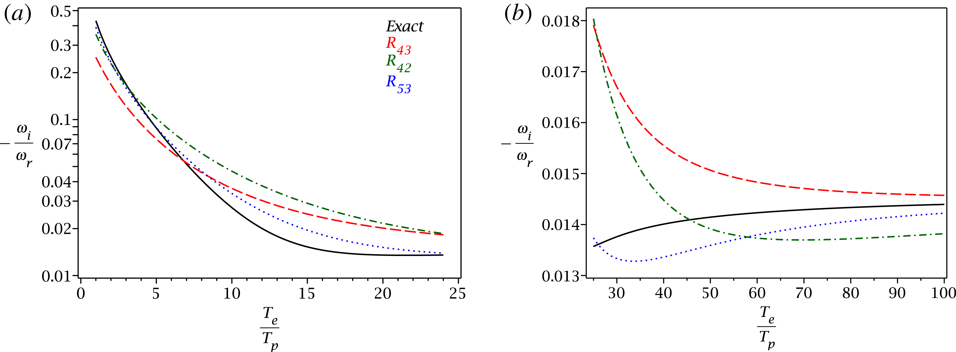
Figure 5. Landau damping of the ion-acoustic (sound) mode. The black solid curve is the solution of exact kinetic dispersion relation (3.366). The other curves are dispersion relations of a fluid model (3.371)–(3.376) where the electron inertia is neglected, supplemented by a closure for
 $r_{\Vert \Vert r}^{(1)}$
. The red dashed line is the
$r_{\Vert \Vert r}^{(1)}$
. The red dashed line is the
 $R_{4,3}(\unicode[STIX]{x1D701})$
closure of Hammett & Perkins (Reference Hammett and Perkins1990), the green dash-dotted line is our new static closure
$R_{4,3}(\unicode[STIX]{x1D701})$
closure of Hammett & Perkins (Reference Hammett and Perkins1990), the green dash-dotted line is our new static closure
 $R_{4,2}(\unicode[STIX]{x1D701})$
and the blue dotted line is the new time-dependent closure
$R_{4,2}(\unicode[STIX]{x1D701})$
and the blue dotted line is the new time-dependent closure
 $R_{5,3}(\unicode[STIX]{x1D701})$
.
$R_{5,3}(\unicode[STIX]{x1D701})$
.
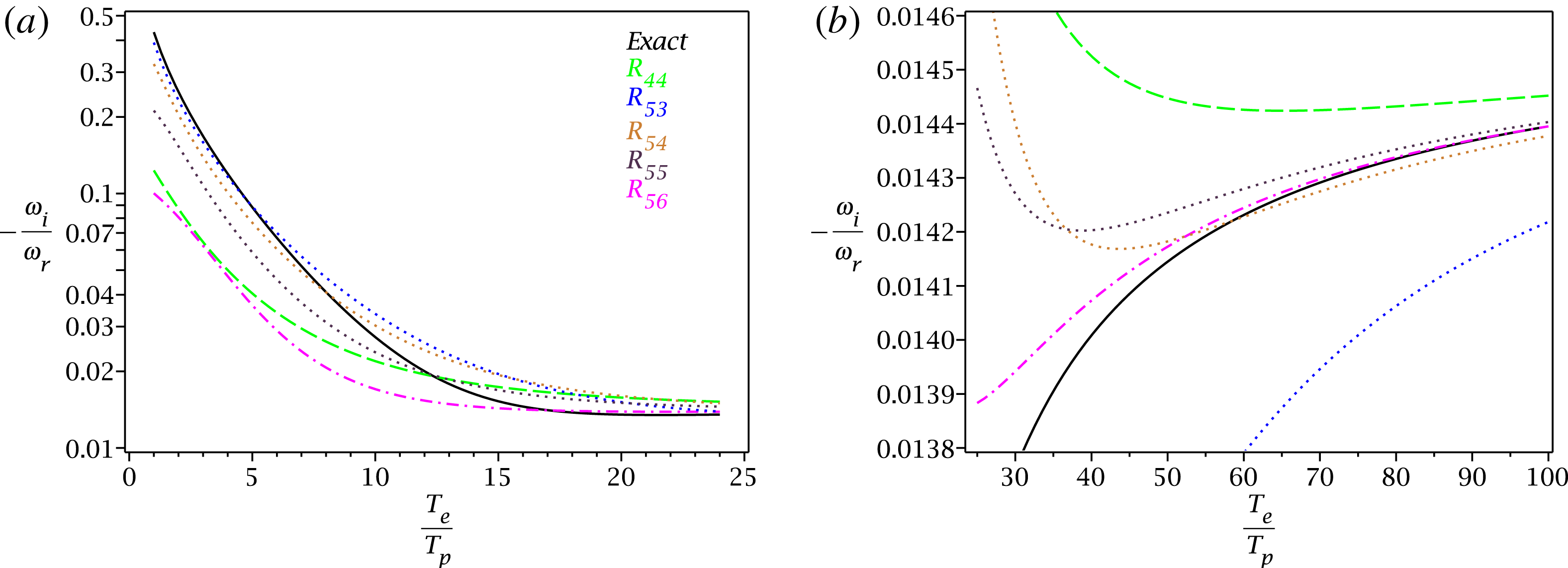
Figure 6. Similar to figure 5, but different closures are compared, and electron inertia is retained. The
 $R_{5,3}(\unicode[STIX]{x1D701})$
closure (blue dotted curve) is kept in the figure so that the comparison to other closures can be done easily. Also, by comparing the
$R_{5,3}(\unicode[STIX]{x1D701})$
closure (blue dotted curve) is kept in the figure so that the comparison to other closures can be done easily. Also, by comparing the
 $R_{5,3}(\unicode[STIX]{x1D701})$
solution with figure 5, it is shown that the effect of electron inertia is negligible. The
$R_{5,3}(\unicode[STIX]{x1D701})$
solution with figure 5, it is shown that the effect of electron inertia is negligible. The
 $R_{4,4}(\unicode[STIX]{x1D701})$
is the only static closure, and all other closures are time dependent.
$R_{4,4}(\unicode[STIX]{x1D701})$
is the only static closure, and all other closures are time dependent.
With the help of Maple software, we analytically investigated dispersion relations of all the obtained fluid closures, and we investigated if the resulting dispersion relation (including the electron inertia) is equivalent to the kinetic result (3.366), after replacing the
 $R(\unicode[STIX]{x1D701})$
with
$R(\unicode[STIX]{x1D701})$
with
 $R_{n,n^{\prime }}(\unicode[STIX]{x1D701})$
, i.e. if the fluid dispersion relation is equivalent to the numerator of
$R_{n,n^{\prime }}(\unicode[STIX]{x1D701})$
, i.e. if the fluid dispersion relation is equivalent to the numerator of

All the closures considered in this subsection satisfied this requirement, however, some other previously obtained closures did not. We concluded that satisfying (3.382) should be indeed considered as a strong requirement for a physically meaningful closure, and closures that did not satisfy this requirement were therefore eliminated. The results are summarized in the § 3.6 ‘Table of moments
 $(u_{\Vert },T_{\Vert },q_{\Vert },\widetilde{r}_{\Vert \Vert })$
for various Padé approximants’, equations (3.241), (3.242).
$(u_{\Vert },T_{\Vert },q_{\Vert },\widetilde{r}_{\Vert \Vert })$
for various Padé approximants’, equations (3.241), (3.242).
3.15 Electron Landau damping of the Langmuir mode
In addition to the ion-acoustic mode, let us calculate the Landau damping for the second (perhaps first) typical example, of how Landau damping is addressed in plasma physics books, the Langmuir mode. Focusing on the electron species and making the proton species cold and ‘very heavy’ with
 $m_{p}\rightarrow \infty$
, i.e. immobile with
$m_{p}\rightarrow \infty$
, i.e. immobile with
 $u_{zp}^{(1)}=0$
, the proton species completely decouples from the system, and their role is just to conserve the leading-order charge neutrality
$u_{zp}^{(1)}=0$
, the proton species completely decouples from the system, and their role is just to conserve the leading-order charge neutrality
 $n_{0p}=n_{0e}=n_{0}$
. Since we have not dealt with such a system so far (not even in Part 1 of the text), let us write down the basic equation nicely in real space in physical units. Neglecting the electron heat flux, the basic system of linearized equations reads
$n_{0p}=n_{0e}=n_{0}$
. Since we have not dealt with such a system so far (not even in Part 1 of the text), let us write down the basic equation nicely in real space in physical units. Neglecting the electron heat flux, the basic system of linearized equations reads
 $$\begin{eqnarray}\displaystyle & \displaystyle \frac{\unicode[STIX]{x2202}n_{e}^{(1)}}{\unicode[STIX]{x2202}t}+n_{0}\unicode[STIX]{x2202}_{z}u_{ze}^{(1)}=0; & \displaystyle\end{eqnarray}$$
 $$\begin{eqnarray}\displaystyle & \displaystyle \frac{\unicode[STIX]{x2202}u_{ze}^{(1)}}{\unicode[STIX]{x2202}t}+\frac{1}{m_{e}n_{0}}\unicode[STIX]{x2202}_{z}p_{\Vert e}^{(1)}+\frac{e}{m_{e}}E_{\Vert }=0; & \displaystyle\end{eqnarray}$$
 $$\begin{eqnarray}\displaystyle & \displaystyle \frac{\unicode[STIX]{x2202}p_{\Vert e}^{(1)}}{\unicode[STIX]{x2202}t}+3p_{\Vert e}^{(0)}\unicode[STIX]{x2202}_{z}u_{ze}^{(1)}=0. & \displaystyle\end{eqnarray}$$
Using the general electrostatic Maxwell equation for the current (including the displacement current)
 $$\begin{eqnarray}\boldsymbol{j}=\mathop{\sum }_{r}q_{r}n_{r}\boldsymbol{u}_{r}=\cancel{\frac{c}{4\unicode[STIX]{x03C0}}\unicode[STIX]{x1D735}\times \boldsymbol{B}}-\frac{1}{4\unicode[STIX]{x03C0}}\frac{\unicode[STIX]{x2202}\boldsymbol{E}}{\unicode[STIX]{x2202}t},\end{eqnarray}$$
that in our specific 1-D linear case considered here reads
 $$\begin{eqnarray}j_{\Vert }=-en_{0}u_{ze}^{(1)}=-\frac{1}{4\unicode[STIX]{x03C0}}\frac{\unicode[STIX]{x2202}E_{\Vert }}{\unicode[STIX]{x2202}t},\end{eqnarray}$$
prescribes the electric field time evolution, and the system of equations is closed. By applying
 $\unicode[STIX]{x2202}/\unicode[STIX]{x2202}t$
to the momentum equation (3.384), the equations can be combined, yielding a wave equation
$\unicode[STIX]{x2202}/\unicode[STIX]{x2202}t$
to the momentum equation (3.384), the equations can be combined, yielding a wave equation
 $$\begin{eqnarray}\left[\frac{\unicode[STIX]{x2202}^{2}}{\unicode[STIX]{x2202}t^{2}}-\frac{3p_{\Vert e}^{(0)}}{m_{e}n_{0}}\unicode[STIX]{x2202}_{z}^{2}+\unicode[STIX]{x1D714}_{pe}^{2}\right]u_{ze}^{(1)}=0,\end{eqnarray}$$
where the electron plasma frequency
 $\unicode[STIX]{x1D714}_{pe}^{2}=4\unicode[STIX]{x03C0}e^{2}n_{0}/m_{e}$
. This wave equation describes the basic plasma physics mode, known as the Langmuir mode, and the dispersion relation is
$\unicode[STIX]{x1D714}_{pe}^{2}=4\unicode[STIX]{x03C0}e^{2}n_{0}/m_{e}$
. This wave equation describes the basic plasma physics mode, known as the Langmuir mode, and the dispersion relation is
 $$\begin{eqnarray}\unicode[STIX]{x1D714}^{2}=\unicode[STIX]{x1D714}_{pe}^{2}+\frac{3T_{\Vert e}^{(0)}}{m_{e}}k_{\Vert }^{2}.\end{eqnarray}$$
If we ignored the displacement current
 $\unicode[STIX]{x2202}E_{\Vert }/\unicode[STIX]{x2202}t$
, the
$\unicode[STIX]{x2202}E_{\Vert }/\unicode[STIX]{x2202}t$
, the
 $\unicode[STIX]{x1D714}_{pe}^{2}$
term would be absent. By dividing with
$\unicode[STIX]{x1D714}_{pe}^{2}$
term would be absent. By dividing with
 $\unicode[STIX]{x1D714}_{pe}^{2}$
and by using the Debye length
$\unicode[STIX]{x1D714}_{pe}^{2}$
and by using the Debye length
 $\unicode[STIX]{x1D706}_{De}=1/k_{De}$
where
$\unicode[STIX]{x1D706}_{De}=1/k_{De}$
where
 $k_{De}^{2}=4\unicode[STIX]{x03C0}e^{2}n_{0e}/T_{\Vert e}^{(0)}$
, so that the Debye length
$k_{De}^{2}=4\unicode[STIX]{x03C0}e^{2}n_{0e}/T_{\Vert e}^{(0)}$
, so that the Debye length
 $\unicode[STIX]{x1D706}_{De}^{2}=T_{\Vert e}^{(0)}/(m_{e}\unicode[STIX]{x1D714}_{pe}^{2})$
, the dispersion relation (3.389) reads
$\unicode[STIX]{x1D706}_{De}^{2}=T_{\Vert e}^{(0)}/(m_{e}\unicode[STIX]{x1D714}_{pe}^{2})$
, the dispersion relation (3.389) reads
 $$\begin{eqnarray}\frac{\unicode[STIX]{x1D714}^{2}}{\unicode[STIX]{x1D714}_{pe}^{2}}=1+3\unicode[STIX]{x1D706}_{De}^{2}k_{\Vert }^{2}.\end{eqnarray}$$
Obviously, the electron plasma frequency and the electron Debye length are the natural normalizing units of this system, and one should use normalized quantities
 $\unicode[STIX]{x1D714}/\unicode[STIX]{x1D714}_{pe}$
and
$\unicode[STIX]{x1D714}/\unicode[STIX]{x1D714}_{pe}$
and
 $k_{\Vert }\unicode[STIX]{x1D706}_{De}$
. A useful relation also is
$k_{\Vert }\unicode[STIX]{x1D706}_{De}$
. A useful relation also is
 $\unicode[STIX]{x1D706}_{De}^{2}=v_{\text{th}\Vert e}^{2}/(2\unicode[STIX]{x1D714}_{pe}^{2}).$
Often, in plasma physics books, the CGL adiabatic index
 $\unicode[STIX]{x1D6FE}_{\Vert }=3$
in the above two equations, is substituted with a general adiabatic index
$\unicode[STIX]{x1D6FE}_{\Vert }=3$
in the above two equations, is substituted with a general adiabatic index
 $\unicode[STIX]{x1D6FE}_{e}$
, so that a more ‘general’ case can be considered. This is especially useful if the Langmuir waves, which are the basic waves of plasma physics, are introduced early on (in an early chapter of a book), where the correct CGL value of
$\unicode[STIX]{x1D6FE}_{e}$
, so that a more ‘general’ case can be considered. This is especially useful if the Langmuir waves, which are the basic waves of plasma physics, are introduced early on (in an early chapter of a book), where the correct CGL value of
 $\unicode[STIX]{x1D6FE}_{\Vert }=3$
is difficult to introduce. Again, we have an advantage of not being a plasma book, and we are not describing the general electrostatic case, we are describing the fully electromagnetic case, but we are focusing only on one mode – the electrostatic mode that propagates parallel to
$\unicode[STIX]{x1D6FE}_{\Vert }=3$
is difficult to introduce. Again, we have an advantage of not being a plasma book, and we are not describing the general electrostatic case, we are describing the fully electromagnetic case, but we are focusing only on one mode – the electrostatic mode that propagates parallel to
 $B_{0}$
. In the view presented here, and as elaborated in Part 1 of the text, playing with adiabatic indices does not make much sense. No adiabatic index can match the CGL and the MHD, the CGL is always different from MHD, even for an isotropic distribution function with
$B_{0}$
. In the view presented here, and as elaborated in Part 1 of the text, playing with adiabatic indices does not make much sense. No adiabatic index can match the CGL and the MHD, the CGL is always different from MHD, even for an isotropic distribution function with
 $T_{\Vert }^{(0)}=T_{\bot }^{(0)}$
. Therefore, we are not introducing any adiabatic index, and the correct CGL value is used, and fixed to 3. Instead, we introduce the electron heat flux and get closer to the kinetic theory in a much more sophisticated way.
$T_{\Vert }^{(0)}=T_{\bot }^{(0)}$
. Therefore, we are not introducing any adiabatic index, and the correct CGL value is used, and fixed to 3. Instead, we introduce the electron heat flux and get closer to the kinetic theory in a much more sophisticated way.
The basic linearized fluid equations in Fourier space read
 $$\begin{eqnarray}\displaystyle & \displaystyle -\unicode[STIX]{x1D714}\frac{n_{e}^{(1)}}{n_{0}}+k_{\Vert }u_{ze}^{(1)}=0; & \displaystyle \nonumber\\ \displaystyle & \displaystyle -\unicode[STIX]{x1D714}u_{ze}^{(1)}+\frac{1}{2}v_{\text{th}\Vert e}^{2}k_{\Vert }\frac{p_{\Vert e}^{(1)}}{p_{\Vert e}^{(0)}}+\frac{1}{2}\frac{v_{\text{th}\Vert e}^{2}}{\unicode[STIX]{x1D706}_{De}^{2}}\frac{u_{ze}^{(1)}}{\unicode[STIX]{x1D714}}=0; & \displaystyle \nonumber\\ \displaystyle & \displaystyle -\unicode[STIX]{x1D714}\frac{p_{\Vert e}^{(1)}}{p_{\Vert e}^{(0)}}+3k_{\Vert }u_{ze}^{(1)}+k_{\Vert }\frac{q_{\Vert e}^{(1)}}{p_{\Vert e}^{(0)}}=0; & \displaystyle\end{eqnarray}$$
 $$\begin{eqnarray}\displaystyle & \displaystyle -\unicode[STIX]{x1D714}\frac{q_{\Vert e}^{(1)}}{p_{\Vert e}^{(0)}}+\frac{3}{2}v_{\text{th}\Vert e}^{2}k_{\Vert }\left(\frac{p_{\Vert e}^{(1)}}{p_{\Vert e}^{(0)}}-\frac{n_{e}^{(1)}}{n_{0}}\right)+k_{\Vert }\frac{\widetilde{r}_{\Vert \Vert e}^{(1)}}{p_{\Vert e}^{(0)}}=0, & \displaystyle\end{eqnarray}$$
and are accompanied for example by the
 $R_{4,3}(\unicode[STIX]{x1D701})$
closure
$R_{4,3}(\unicode[STIX]{x1D701})$
closure
 $$\begin{eqnarray}\frac{\widetilde{r}_{\Vert \Vert e}^{(1)}}{p_{\Vert e}^{(0)}}=\frac{32-9\unicode[STIX]{x03C0}}{2(3\unicode[STIX]{x03C0}-8)}v_{\text{th}\Vert e}^{2}\left(\frac{p_{\Vert e}^{(1)}}{p_{\Vert e}^{(0)}}-\frac{n_{e}^{(1)}}{n_{0}}\right)-\frac{2\sqrt{\unicode[STIX]{x03C0}}}{3\unicode[STIX]{x03C0}-8}v_{\text{th}\Vert e}i\text{sign}(k_{\Vert })\frac{q_{\Vert e}^{(1)}}{p_{\Vert e}^{(0)}}.\end{eqnarray}$$
The dispersion relation of this fluid model reads (suppressing
 $e$
in the electron Debye length
$e$
in the electron Debye length
 $\unicode[STIX]{x1D706}_{De}$
)
$\unicode[STIX]{x1D706}_{De}$
)
 $$\begin{eqnarray}\unicode[STIX]{x1D701}_{e}^{4}+\frac{2i\sqrt{\unicode[STIX]{x03C0}}}{3\unicode[STIX]{x03C0}-8}\unicode[STIX]{x1D701}_{e}^{3}-\frac{3\unicode[STIX]{x03C0}-8+(9\unicode[STIX]{x03C0}-16)k_{\Vert }^{2}\unicode[STIX]{x1D706}_{D}^{2}}{2(3\unicode[STIX]{x03C0}-8)k_{\Vert }^{2}\unicode[STIX]{x1D706}_{D}^{2}}\unicode[STIX]{x1D701}_{e}^{2}-\frac{i\sqrt{\unicode[STIX]{x03C0}}(1+3k_{\Vert }^{2}\unicode[STIX]{x1D706}_{D}^{2})}{(3\unicode[STIX]{x03C0}-8)k_{\Vert }^{2}\unicode[STIX]{x1D706}_{D}^{2}}\unicode[STIX]{x1D701}_{e}+\frac{2(1+k_{\Vert }^{2}\unicode[STIX]{x1D706}_{D}^{2})}{(3\unicode[STIX]{x03C0}-8)k_{\Vert }^{2}\unicode[STIX]{x1D706}_{D}^{2}}=0,\end{eqnarray}$$
where
 $$\begin{eqnarray}\unicode[STIX]{x1D701}_{e}=\frac{\unicode[STIX]{x1D714}}{|k_{\Vert }|v_{\text{th}\Vert e}}=\frac{\unicode[STIX]{x1D714}}{\unicode[STIX]{x1D714}_{pe}}\frac{1}{\sqrt{2}|k_{\Vert }|\unicode[STIX]{x1D706}_{D}}.\end{eqnarray}$$
The exact kinetic dispersion relation reads
As can be verified, the fluid dispersion relation (3.394) is equivalent to the kinetic one, if
 $R(\unicode[STIX]{x1D701}_{e})$
is replaced by
$R(\unicode[STIX]{x1D701}_{e})$
is replaced by
 $R_{4,3}(\unicode[STIX]{x1D701}_{e})$
.
$R_{4,3}(\unicode[STIX]{x1D701}_{e})$
.
Using the static
 $R_{4,2}(\unicode[STIX]{x1D701})$
closure, the dispersion relation reads
$R_{4,2}(\unicode[STIX]{x1D701})$
closure, the dispersion relation reads
 $$\begin{eqnarray}\displaystyle & & \displaystyle \unicode[STIX]{x1D701}_{e}^{4}+i\sqrt{\unicode[STIX]{x03C0}}\frac{10-3\unicode[STIX]{x03C0}}{16-5\unicode[STIX]{x03C0}}\unicode[STIX]{x1D701}_{e}^{3}-\frac{16-5\unicode[STIX]{x03C0}+(32-9\unicode[STIX]{x03C0})k_{\Vert }^{2}\unicode[STIX]{x1D706}_{D}^{2}}{2(16-5\unicode[STIX]{x03C0})k_{\Vert }^{2}\unicode[STIX]{x1D706}_{D}^{2}}\unicode[STIX]{x1D701}_{e}^{2}\nonumber\\ \displaystyle & & \displaystyle \qquad -\,i\sqrt{\unicode[STIX]{x03C0}}\frac{10-3\unicode[STIX]{x03C0}+2k_{\Vert }^{2}\unicode[STIX]{x1D706}_{D}^{2}}{2(16-5\unicode[STIX]{x03C0})k_{\Vert }^{2}\unicode[STIX]{x1D706}_{D}^{2}}\unicode[STIX]{x1D701}_{e}+\frac{(3\unicode[STIX]{x03C0}-8)(1+k_{\Vert }^{2}\unicode[STIX]{x1D706}_{D}^{2})}{2(16-5\unicode[STIX]{x03C0})k_{\Vert }^{2}\unicode[STIX]{x1D706}_{D}^{2}}=0,\end{eqnarray}$$
using the static
 $R_{4,4}(\unicode[STIX]{x1D701})$
closure yields
$R_{4,4}(\unicode[STIX]{x1D701})$
closure yields
 $$\begin{eqnarray}\displaystyle \unicode[STIX]{x1D701}_{e}^{4}+i\sqrt{\unicode[STIX]{x03C0}}\frac{3}{4}\unicode[STIX]{x1D701}_{e}^{3}-\frac{1+6k_{\Vert }^{2}\unicode[STIX]{x1D706}_{D}^{2}}{2k_{\Vert }^{2}\unicode[STIX]{x1D706}_{D}^{2}}\unicode[STIX]{x1D701}_{e}^{2}-i\sqrt{\unicode[STIX]{x03C0}}\frac{3(1+3k_{\Vert }^{2}\unicode[STIX]{x1D706}_{D}^{2})}{8k_{\Vert }^{2}\unicode[STIX]{x1D706}_{D}^{2}}\unicode[STIX]{x1D701}_{e}+\frac{3(1+k_{\Vert }^{2}\unicode[STIX]{x1D706}_{D}^{2})}{4k_{\Vert }^{2}\unicode[STIX]{x1D706}_{D}^{2}}=0, & & \displaystyle\end{eqnarray}$$
and the simplest static
 $R_{3,2}(\unicode[STIX]{x1D701})$
closure yields
$R_{3,2}(\unicode[STIX]{x1D701})$
closure yields
 $$\begin{eqnarray}\displaystyle \unicode[STIX]{x1D701}_{e}^{3}+\frac{2i}{\sqrt{\unicode[STIX]{x03C0}}}\unicode[STIX]{x1D701}_{e}^{2}-\frac{1+3k_{\Vert }^{2}\unicode[STIX]{x1D706}_{D}^{2}}{2k_{\Vert }^{2}\unicode[STIX]{x1D706}_{D}^{2}}\unicode[STIX]{x1D701}_{e}-\frac{i(1+k_{\Vert }^{2}\unicode[STIX]{x1D706}_{D}^{2})}{\sqrt{\unicode[STIX]{x03C0}}k_{\Vert }^{2}\unicode[STIX]{x1D706}_{D}^{2}}=0. & & \displaystyle\end{eqnarray}$$
All dispersion relations are fully consistent with the kinetic dispersion relation (3.396) when
 $R(\unicode[STIX]{x1D701}_{e})$
is replaced by the corresponding
$R(\unicode[STIX]{x1D701}_{e})$
is replaced by the corresponding
 $R_{4,2}(\unicode[STIX]{x1D701}_{e})$
,
$R_{4,2}(\unicode[STIX]{x1D701}_{e})$
,
 $R_{4,4}(\unicode[STIX]{x1D701}_{e})$
and
$R_{4,4}(\unicode[STIX]{x1D701}_{e})$
and
 $R_{3,2}(\unicode[STIX]{x1D701}_{e})$
(equivalent to the numerator of the resulting expression). We verified that this is also true for the static closure
$R_{3,2}(\unicode[STIX]{x1D701}_{e})$
(equivalent to the numerator of the resulting expression). We verified that this is also true for the static closure
 $R_{3,1}(\unicode[STIX]{x1D701}_{e})$
and actually all the ‘reliable’ closures marked in (3.241), (3.242) with ‘
$R_{3,1}(\unicode[STIX]{x1D701}_{e})$
and actually all the ‘reliable’ closures marked in (3.241), (3.242) with ‘
 ${\checkmark}$
’, including the time-dependent closures
${\checkmark}$
’, including the time-dependent closures
 $R_{3,2}(\unicode[STIX]{x1D701}_{e})$
,
$R_{3,2}(\unicode[STIX]{x1D701}_{e})$
,
 $R_{4,2}(\unicode[STIX]{x1D701}_{e})$
,
$R_{4,2}(\unicode[STIX]{x1D701}_{e})$
,
 $R_{4,3}(\unicode[STIX]{x1D701}_{e})$
,
$R_{4,3}(\unicode[STIX]{x1D701}_{e})$
,
 $R_{4,4}(\unicode[STIX]{x1D701}_{e})$
,
$R_{4,4}(\unicode[STIX]{x1D701}_{e})$
,
 $R_{5,3}(\unicode[STIX]{x1D701}_{e})$
,
$R_{5,3}(\unicode[STIX]{x1D701}_{e})$
,
 $R_{5,4}(\unicode[STIX]{x1D701}_{e})$
,
$R_{5,4}(\unicode[STIX]{x1D701}_{e})$
,
 $R_{5,5}(\unicode[STIX]{x1D701}_{e})$
,
$R_{5,5}(\unicode[STIX]{x1D701}_{e})$
,
 $R_{5,6}(\unicode[STIX]{x1D701}_{e})$
. To clearly understand the obtained solutions, let us solve the simple
$R_{5,6}(\unicode[STIX]{x1D701}_{e})$
. To clearly understand the obtained solutions, let us solve the simple
 $R_{3,2}(\unicode[STIX]{x1D701}_{e})$
dispersion relation (3.399) for a few values of
$R_{3,2}(\unicode[STIX]{x1D701}_{e})$
dispersion relation (3.399) for a few values of
 $k_{\Vert }\unicode[STIX]{x1D706}_{D}$
,
$k_{\Vert }\unicode[STIX]{x1D706}_{D}$
,

The first mode is the Langmuir mode, and the second mode is a purely damped higher-order mode. In the complete limit
 $k_{\Vert }\unicode[STIX]{x1D706}_{D}\rightarrow 0$
, the Langmuir mode becomes undamped with a solution
$k_{\Vert }\unicode[STIX]{x1D706}_{D}\rightarrow 0$
, the Langmuir mode becomes undamped with a solution
 $\unicode[STIX]{x1D701}_{e}=1/(\sqrt{2}|k_{\Vert }|\unicode[STIX]{x1D706}_{D})$
, which corresponds to oscillations with electron plasma frequency
$\unicode[STIX]{x1D701}_{e}=1/(\sqrt{2}|k_{\Vert }|\unicode[STIX]{x1D706}_{D})$
, which corresponds to oscillations with electron plasma frequency
 $\unicode[STIX]{x1D714}=\unicode[STIX]{x1D714}_{pe}$
; and the higher-order mode has a solution
$\unicode[STIX]{x1D714}=\unicode[STIX]{x1D714}_{pe}$
; and the higher-order mode has a solution
 $\unicode[STIX]{x1D701}_{e}=-2i/\sqrt{\unicode[STIX]{x03C0}}$
. Considering the weak damping limit
$\unicode[STIX]{x1D701}_{e}=-2i/\sqrt{\unicode[STIX]{x03C0}}$
. Considering the weak damping limit
 $\unicode[STIX]{x1D701}_{e}=x+iy$
, where
$\unicode[STIX]{x1D701}_{e}=x+iy$
, where
 $x\gg y$
, at the leading order
$x\gg y$
, at the leading order
 $\unicode[STIX]{x1D701}_{e}^{2}=x^{2}+i2xy$
and
$\unicode[STIX]{x1D701}_{e}^{2}=x^{2}+i2xy$
and
 $\unicode[STIX]{x1D701}_{e}^{3}=x^{3}+i3x^{2}y$
, which when used in the dispersion relation (3.399) that is separated into real and imaginary parts yields
$\unicode[STIX]{x1D701}_{e}^{3}=x^{3}+i3x^{2}y$
, which when used in the dispersion relation (3.399) that is separated into real and imaginary parts yields
 $$\begin{eqnarray}\displaystyle & & \displaystyle x^{3}-\frac{4}{\sqrt{\unicode[STIX]{x03C0}}}xy-\frac{1+3k_{\Vert }^{2}\unicode[STIX]{x1D706}_{D}^{2}}{2k_{\Vert }^{2}\unicode[STIX]{x1D706}_{D}^{2}}x=0;\nonumber\\ \displaystyle & & \displaystyle 3x^{2}y+\frac{2}{\sqrt{\unicode[STIX]{x03C0}}}x^{2}-\frac{1+3k_{\Vert }^{2}\unicode[STIX]{x1D706}_{D}^{2}}{2k_{\Vert }^{2}\unicode[STIX]{x1D706}_{D}^{2}}y-\frac{1}{\sqrt{\unicode[STIX]{x03C0}}}\frac{1+k_{\Vert }^{2}\unicode[STIX]{x1D706}_{D}^{2}}{k_{\Vert }^{2}\unicode[STIX]{x1D706}_{D}^{2}}=0,\nonumber\end{eqnarray}$$
and for
 $x\gg y$
at the leading order
$x\gg y$
at the leading order
 $$\begin{eqnarray}\displaystyle x^{2}=\frac{1+3k_{\Vert }^{2}\unicode[STIX]{x1D706}_{D}^{2}}{2k_{\Vert }^{2}\unicode[STIX]{x1D706}_{D}^{2}};\quad y=-\frac{1}{\sqrt{\unicode[STIX]{x03C0}}x^{2}}=-\frac{2}{\sqrt{\unicode[STIX]{x03C0}}}\frac{k_{\Vert }^{2}\unicode[STIX]{x1D706}_{D}^{2}}{(1+3k_{\Vert }^{2}\unicode[STIX]{x1D706}_{D}^{2})}, & & \displaystyle\end{eqnarray}$$
which approximates the above numerical solutions reasonably well up to let us say
 $k_{\Vert }\unicode[STIX]{x1D706}_{D}=0.3$
, and from (3.395) the
$k_{\Vert }\unicode[STIX]{x1D706}_{D}=0.3$
, and from (3.395) the
 $x,y$
expressions are equivalent to
$x,y$
expressions are equivalent to
 $$\begin{eqnarray}\unicode[STIX]{x1D714}_{r}^{2}=\unicode[STIX]{x1D714}_{pe}^{2}(1+3k_{\Vert }^{2}\unicode[STIX]{x1D706}_{D}^{2});\quad \unicode[STIX]{x1D714}_{i}=-\sqrt{\frac{8}{\unicode[STIX]{x03C0}}}\frac{|k_{\Vert }|^{3}\unicode[STIX]{x1D706}_{D}^{3}}{1+3k_{\Vert }^{2}\unicode[STIX]{x1D706}_{D}^{2}}\unicode[STIX]{x1D714}_{pe}.\end{eqnarray}$$
For
 $k_{\Vert }\unicode[STIX]{x1D706}_{D}\ll 1$
, the Landau damping of the Langmuir mode goes to zero, however, the damping rate is very overestimated. The approximate kinetic result found in plasma books (see for example Gurnett & Bhattacharjee (Reference Gurnett and Bhattacharjee2005), page 349) has of course the same real frequency, however, the damping rate reads
$k_{\Vert }\unicode[STIX]{x1D706}_{D}\ll 1$
, the Landau damping of the Langmuir mode goes to zero, however, the damping rate is very overestimated. The approximate kinetic result found in plasma books (see for example Gurnett & Bhattacharjee (Reference Gurnett and Bhattacharjee2005), page 349) has of course the same real frequency, however, the damping rate reads
 $$\begin{eqnarray}\unicode[STIX]{x1D714}_{r}^{2}=\unicode[STIX]{x1D714}_{pe}^{2}(1+3k_{\Vert }^{2}\unicode[STIX]{x1D706}_{D}^{2});\quad \unicode[STIX]{x1D714}_{i}=-\sqrt{\frac{\unicode[STIX]{x03C0}}{8}}\frac{\unicode[STIX]{x1D714}_{pe}}{|k_{\Vert }|^{3}\unicode[STIX]{x1D706}_{D}^{3}}e^{-1+3k_{\Vert }^{2}\unicode[STIX]{x1D706}_{D}^{2}/2k_{\Vert }^{2}\unicode[STIX]{x1D706}_{D}^{2}}.\end{eqnarray}$$
Since
 $k_{\Vert }\unicode[STIX]{x1D706}_{D}\ll 1$
, Landau (Reference Landau1946) writes (see his equations (16) and (17))
$k_{\Vert }\unicode[STIX]{x1D706}_{D}\ll 1$
, Landau (Reference Landau1946) writes (see his equations (16) and (17))
 $$\begin{eqnarray}\unicode[STIX]{x1D714}_{r}=\unicode[STIX]{x1D714}_{pe}\left(1+\frac{3}{2}k_{\Vert }^{2}\unicode[STIX]{x1D706}_{D}^{2}\right);\quad \unicode[STIX]{x1D714}_{i}=-\sqrt{\frac{\unicode[STIX]{x03C0}}{8}}\frac{\unicode[STIX]{x1D714}_{pe}}{|k_{\Vert }|^{3}\unicode[STIX]{x1D706}_{D}^{3}}e^{-1/2k_{\Vert }^{2}\unicode[STIX]{x1D706}_{D}^{2}}.\end{eqnarray}$$
For
 $k_{\Vert }\unicode[STIX]{x1D706}_{D}\ll 1$
, i.e. approaching long wavelengths, the exponential term suppresses the Landau damping much quicker than our result (3.401). To understand the discrepancy, let us quickly consider how the kinetic result (3.402) was obtained. The result is obtained by considering asymptotic expansion
$k_{\Vert }\unicode[STIX]{x1D706}_{D}\ll 1$
, i.e. approaching long wavelengths, the exponential term suppresses the Landau damping much quicker than our result (3.401). To understand the discrepancy, let us quickly consider how the kinetic result (3.402) was obtained. The result is obtained by considering asymptotic expansion
 $|\unicode[STIX]{x1D701}_{e}|\gg 1$
of the exact kinetic dispersion relation (3.396), which in the weak growth-rate approximation (see (3.67) with
$|\unicode[STIX]{x1D701}_{e}|\gg 1$
of the exact kinetic dispersion relation (3.396), which in the weak growth-rate approximation (see (3.67) with
 $\unicode[STIX]{x1D70E}=1$
) reads
$\unicode[STIX]{x1D70E}=1$
) reads
 $$\begin{eqnarray}1+\frac{1}{k_{\Vert }^{2}\unicode[STIX]{x1D706}_{D}^{2}}\left[-\frac{1}{2\unicode[STIX]{x1D701}_{e}^{2}}-\frac{3}{4\unicode[STIX]{x1D701}_{e}^{4}}+i\sqrt{\unicode[STIX]{x03C0}}\unicode[STIX]{x1D701}_{e}e^{-\unicode[STIX]{x1D701}_{e}^{2}}\right]=0.\end{eqnarray}$$
Using
 $\unicode[STIX]{x1D701}_{e}=x+iy$
with
$\unicode[STIX]{x1D701}_{e}=x+iy$
with
 $x\gg y$
and
$x\gg y$
and
 $k_{\Vert }\unicode[STIX]{x1D706}_{D}\ll 1$
yields at the leading order
$k_{\Vert }\unicode[STIX]{x1D706}_{D}\ll 1$
yields at the leading order
 $x^{2}=(1+3k_{\Vert }^{2}\unicode[STIX]{x1D706}_{D}^{2})/2k_{\Vert }^{2}\unicode[STIX]{x1D706}_{D}^{2}$
which agrees with (3.400) and the damping rate is
$x^{2}=(1+3k_{\Vert }^{2}\unicode[STIX]{x1D706}_{D}^{2})/2k_{\Vert }^{2}\unicode[STIX]{x1D706}_{D}^{2}$
which agrees with (3.400) and the damping rate is
 $y=-\sqrt{\unicode[STIX]{x03C0}}x^{4}e^{-x^{2}}$
, which recovers (3.402). The
$y=-\sqrt{\unicode[STIX]{x03C0}}x^{4}e^{-x^{2}}$
, which recovers (3.402). The
 $e^{-x^{2}}$
term in the damping rate comes from the last term in (3.404), and as discussed previously, this term is neglected in the asymptotic expansion when constructing the Padé approximants of
$e^{-x^{2}}$
term in the damping rate comes from the last term in (3.404), and as discussed previously, this term is neglected in the asymptotic expansion when constructing the Padé approximants of
 $R(\unicode[STIX]{x1D701})$
(it is however included in the power-series expansion), explaining the discrepancy.
$R(\unicode[STIX]{x1D701})$
(it is however included in the power-series expansion), explaining the discrepancy.
The damping rate of the Langmuir mode is plotted in figure 7 and the real frequency in figure 8, where solutions of various fluid models are compared with exact kinetic dispersion relation (3.396), depicted as the black solid line. Additionally, the asymptotic kinetic solution (3.402) from plasma physics books is plotted as the black dotted line. Figure 7 is plotted in log–log scale and figure 8 uses linear scales. It is shown that for
 $k_{\Vert }\unicode[STIX]{x1D706}_{D}>0.2$
, fluid models can reproduce the damping of the Langmuir mode quite accurately, and the most accurate closure is
$k_{\Vert }\unicode[STIX]{x1D706}_{D}>0.2$
, fluid models can reproduce the damping of the Langmuir mode quite accurately, and the most accurate closure is
 $R_{5,3}(\unicode[STIX]{x1D701})$
. This closure also reproduces the real frequency of the Langmuir mode very accurately and actually better than the asymptotic kinetic solution (3.402).
$R_{5,3}(\unicode[STIX]{x1D701})$
. This closure also reproduces the real frequency of the Langmuir mode very accurately and actually better than the asymptotic kinetic solution (3.402).
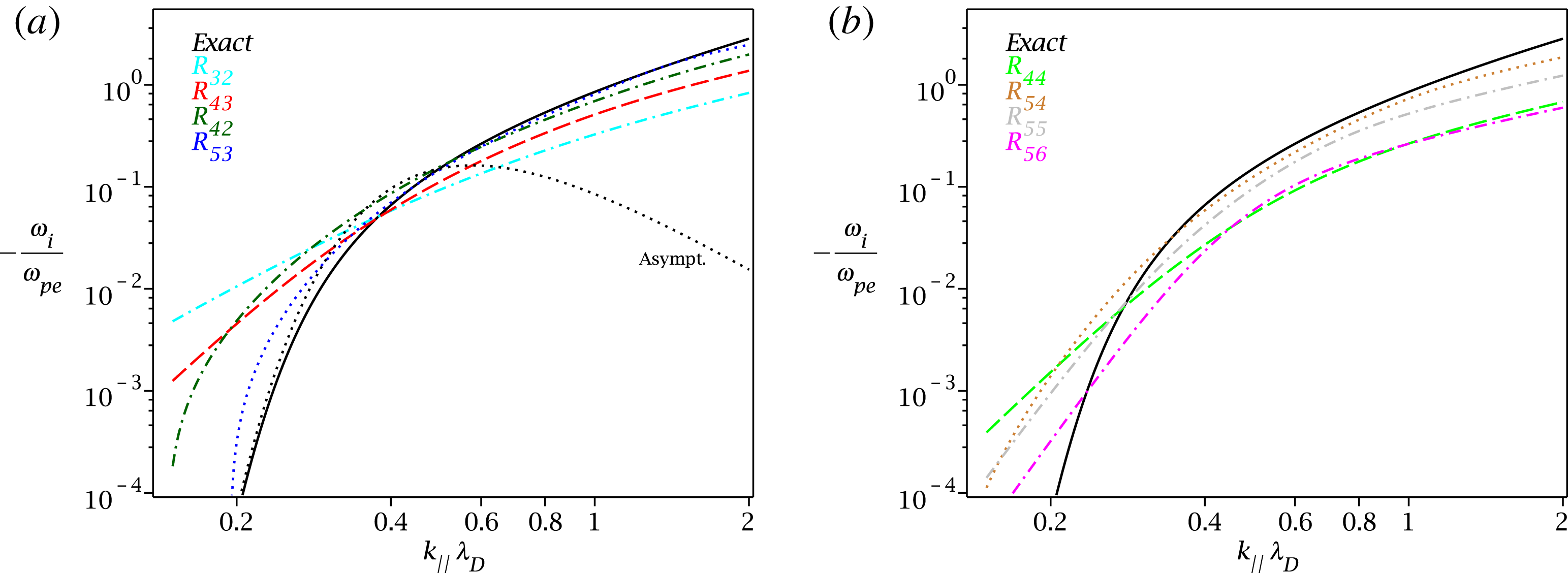
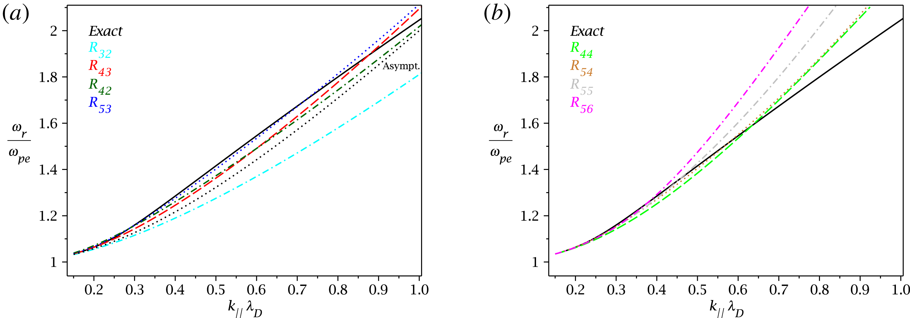
Figure 8. Real frequency of the Langmuir mode.
Nevertheless, as discussed above, because of the missing exponential factor in fluid models, the Landau damping becomes very overestimated at scales
 $k_{\Vert }\unicode[STIX]{x1D706}_{D}<0.2$
, i.e. it is the long-wavelength limit (and not the short-wavelength limit) that represents trouble. This is because in the long-wavelength limit, the frequency of Langmuir mode does not go to zero but approaches the electron plasma frequency
$k_{\Vert }\unicode[STIX]{x1D706}_{D}<0.2$
, i.e. it is the long-wavelength limit (and not the short-wavelength limit) that represents trouble. This is because in the long-wavelength limit, the frequency of Langmuir mode does not go to zero but approaches the electron plasma frequency
 $\unicode[STIX]{x1D714}_{pe}$
, and so the phase speed
$\unicode[STIX]{x1D714}_{pe}$
, and so the phase speed
 $\unicode[STIX]{x1D714}_{r}/k_{\Vert }$
(and the variable
$\unicode[STIX]{x1D714}_{r}/k_{\Vert }$
(and the variable
 $\unicode[STIX]{x1D701}_{e}$
) becomes large and for
$\unicode[STIX]{x1D701}_{e}$
) becomes large and for
 $k_{\Vert }\unicode[STIX]{x1D706}_{D}\rightarrow 0$
goes to infinity, where the fluid closures become imprecise. Landau fluid simulations of the Langmuir mode should be therefore restricted to scales
$k_{\Vert }\unicode[STIX]{x1D706}_{D}\rightarrow 0$
goes to infinity, where the fluid closures become imprecise. Landau fluid simulations of the Langmuir mode should be therefore restricted to scales
 $k_{\Vert }\unicode[STIX]{x1D706}_{D}>0.2$
. At longer wavelengths, some closures can actually become ill posed and instead of Landau damping, can produce a small positive growth rate. For example, if one insists on numerical simulations in the domain below
$k_{\Vert }\unicode[STIX]{x1D706}_{D}>0.2$
. At longer wavelengths, some closures can actually become ill posed and instead of Landau damping, can produce a small positive growth rate. For example, if one insists on numerical simulations in the domain below
 $k_{\Vert }\unicode[STIX]{x1D706}_{D}<0.2$
, the closures that have to be eliminated are closures
$k_{\Vert }\unicode[STIX]{x1D706}_{D}<0.2$
, the closures that have to be eliminated are closures
 $R_{4,2}(\unicode[STIX]{x1D701}),R_{5,3}(\unicode[STIX]{x1D701}),R_{5,4}(\unicode[STIX]{x1D701})$
, since they produce a small positive growth rate. We briefly checked, and all other closures seems to be well behaved all the way up to
$R_{4,2}(\unicode[STIX]{x1D701}),R_{5,3}(\unicode[STIX]{x1D701}),R_{5,4}(\unicode[STIX]{x1D701})$
, since they produce a small positive growth rate. We briefly checked, and all other closures seems to be well behaved all the way up to
 $k_{\Vert }\unicode[STIX]{x1D706}_{D}=10^{-4}$
. At even longer scales, such as
$k_{\Vert }\unicode[STIX]{x1D706}_{D}=10^{-4}$
. At even longer scales, such as
 $k_{\Vert }\unicode[STIX]{x1D706}_{D}=10^{-5}$
, two other closures become ill posed, the
$k_{\Vert }\unicode[STIX]{x1D706}_{D}=10^{-5}$
, two other closures become ill posed, the
 $R_{5,5}(\unicode[STIX]{x1D701})$
and
$R_{5,5}(\unicode[STIX]{x1D701})$
and
 $R_{5,6}(\unicode[STIX]{x1D701})$
, and the remaining closures
$R_{5,6}(\unicode[STIX]{x1D701})$
, and the remaining closures
 $R_{3,1}(\unicode[STIX]{x1D701}),R_{3,2}(\unicode[STIX]{x1D701}),R_{4,3}(\unicode[STIX]{x1D701}),R_{4,4}(\unicode[STIX]{x1D701})$
do not appear to have a length-scale restriction. It is useful to note that this is not only a problem of Landau fluid closures, but at long wavelengths, it is actually the kinetic theory itself that becomes very difficult to solve, and in the region
$R_{3,1}(\unicode[STIX]{x1D701}),R_{3,2}(\unicode[STIX]{x1D701}),R_{4,3}(\unicode[STIX]{x1D701}),R_{4,4}(\unicode[STIX]{x1D701})$
do not appear to have a length-scale restriction. It is useful to note that this is not only a problem of Landau fluid closures, but at long wavelengths, it is actually the kinetic theory itself that becomes very difficult to solve, and in the region
 $k_{\Vert }\unicode[STIX]{x1D706}_{D}<0.1$
, we were often not able to obtain correct numerical solution when solving the exact dispersion relation (3.396).
$k_{\Vert }\unicode[STIX]{x1D706}_{D}<0.1$
, we were often not able to obtain correct numerical solution when solving the exact dispersion relation (3.396).
3.16 Selected closures for the fifth-order moment
Let us work in the 1-D geometry and continue with the hierarchy. In Part 1 of this text, we called the
 $n$
th-order moment
$n$
th-order moment
 $X^{(n)}$
. However, when linearizing, we want to use our
$X^{(n)}$
. However, when linearizing, we want to use our
 $(1)$
superscript as before. Therefore, here we move the
$(1)$
superscript as before. Therefore, here we move the
 $(n)$
index of the
$(n)$
index of the
 $n$
th-order moment down, and refer to the
$n$
th-order moment down, and refer to the
 $n$
th moment simply as
$n$
th moment simply as
 $X_{n}$
. The fifth-order moment
$X_{n}$
. The fifth-order moment
 $X_{5}=m\int (v-u)^{5}f\,\text{d}v$
is linearized according to
$X_{5}=m\int (v-u)^{5}f\,\text{d}v$
is linearized according to
 $$\begin{eqnarray}X_{5}^{(1)}=m\int v^{5}f^{(1)}\,\text{d}v-5u^{(1)}\underbrace{m\int v^{4}f_{0}\,\text{d}v}_{r_{0}},\end{eqnarray}$$
and direct calculation yields (dropping species index
 $r$
everywhere except on charge
$r$
everywhere except on charge
 $q_{r}$
)
$q_{r}$
)
 $$\begin{eqnarray}X_{5}^{(1)}=-q_{r}\unicode[STIX]{x1D6F7}\sqrt{\frac{2T^{(0)}}{m}}\frac{p_{0}}{m}\text{sign}(k_{\Vert })\left(3\unicode[STIX]{x1D701}+2\unicode[STIX]{x1D701}^{3}+4\unicode[STIX]{x1D701}^{5}R(\unicode[STIX]{x1D701})-15\unicode[STIX]{x1D701}R(\unicode[STIX]{x1D701})\right),\end{eqnarray}$$
and alternatively
 $p_{0}/m=n_{0}v_{\text{th}}^{2}/2$
.
$p_{0}/m=n_{0}v_{\text{th}}^{2}/2$
.
The most precise (power-series) static closure can be constructed with the
 $R_{5,3}(\unicode[STIX]{x1D701})$
approximant
$R_{5,3}(\unicode[STIX]{x1D701})$
approximant
 $$\begin{eqnarray}\displaystyle R_{5,3}(\unicode[STIX]{x1D701}):\quad X_{5}^{(1)} & = & \displaystyle -\frac{(104-33\unicode[STIX]{x03C0})\sqrt{\unicode[STIX]{x03C0}}}{2(9\unicode[STIX]{x03C0}^{2}-69\unicode[STIX]{x03C0}+128)}i\text{sign}(k_{\Vert })v_{\text{th}}\widetilde{r}^{(1)}-\frac{(81\unicode[STIX]{x03C0}-256)}{2(9\unicode[STIX]{x03C0}^{2}-69\unicode[STIX]{x03C0}+128)}v_{\text{th}}^{2}q^{(1)}\nonumber\\ \displaystyle & & \displaystyle -\,\frac{3(160-51\unicode[STIX]{x03C0})\sqrt{\unicode[STIX]{x03C0}}}{4(9\unicode[STIX]{x03C0}^{2}-69\unicode[STIX]{x03C0}+128)}i\text{sign}(k_{\Vert })v_{\text{th}}^{3}n_{0}T^{(1)}\nonumber\\ \displaystyle & & \displaystyle -\,\frac{(135\unicode[STIX]{x03C0}^{2}-750\unicode[STIX]{x03C0}+1024)}{2(9\unicode[STIX]{x03C0}^{2}-69\unicode[STIX]{x03C0}+128)}v_{\text{th}}^{2}n_{0}T^{(0)}u^{(1)},\end{eqnarray}$$
and other static closures with the
 $R_{5,4}(\unicode[STIX]{x1D701})$
approximant
$R_{5,4}(\unicode[STIX]{x1D701})$
approximant
 $$\begin{eqnarray}\displaystyle R_{5,4}(\unicode[STIX]{x1D701}):\quad X_{5}^{(1)} & = & \displaystyle -\frac{(21\unicode[STIX]{x03C0}-64)}{(9\unicode[STIX]{x03C0}-28)\sqrt{\unicode[STIX]{x03C0}}}i\text{sign}(k_{\Vert })v_{\text{th}}\widetilde{r}^{(1)}+\frac{(45\unicode[STIX]{x03C0}-136)}{2(9\unicode[STIX]{x03C0}-28)}v_{\text{th}}^{2}q^{(1)}\nonumber\\ \displaystyle & & \displaystyle +\,\frac{(256-81\unicode[STIX]{x03C0})}{2(9\unicode[STIX]{x03C0}-28)\sqrt{\unicode[STIX]{x03C0}}}i\text{sign}(k_{\Vert })n_{0}v_{\text{th}}^{3}T^{(1)},\end{eqnarray}$$
with the
 $R_{5,5}(\unicode[STIX]{x1D701})$
approximant
$R_{5,5}(\unicode[STIX]{x1D701})$
approximant
 $$\begin{eqnarray}\displaystyle R_{5,5}(\unicode[STIX]{x1D701}):\quad X_{5}^{(1)} & = & \displaystyle \frac{6\sqrt{\unicode[STIX]{x03C0}}}{(9\unicode[STIX]{x03C0}-32)}i\text{sign}(k_{\Vert })v_{\text{th}}\widetilde{r}^{(1)}+\frac{3(15\unicode[STIX]{x03C0}-64)}{2(9\unicode[STIX]{x03C0}-32)}v_{\text{th}}^{2}q^{(1)},\end{eqnarray}$$
and with the
 $R_{5,6}(\unicode[STIX]{x1D701})$
approximant
$R_{5,6}(\unicode[STIX]{x1D701})$
approximant
 $$\begin{eqnarray}\displaystyle R_{5,6}(\unicode[STIX]{x1D701}):\quad X_{5}^{(1)} & = & \displaystyle -\frac{8}{3\sqrt{\unicode[STIX]{x03C0}}}i\text{sign}(k_{\Vert })v_{\text{th}}\widetilde{r}^{(1)}+5v_{\text{th}}^{2}q^{(1)}.\end{eqnarray}$$
In Part 1 of this guide, we derived directly from fluid hierarchy that at the linear level
 $$\begin{eqnarray}\frac{\unicode[STIX]{x2202}}{\unicode[STIX]{x2202}t}\widetilde{r}^{(1)}+\unicode[STIX]{x2202}_{z}X_{5}^{(1)}-3v_{\text{th}}^{2}\unicode[STIX]{x2202}_{z}q^{(1)}=0.\end{eqnarray}$$
Now, importantly, by using this equation, it is directly shown that the above static closures with
 $X_{5}^{(1)}$
, are equivalent to time-dependent (dynamic) closures with
$X_{5}^{(1)}$
, are equivalent to time-dependent (dynamic) closures with
 $\widetilde{r}^{(1)}$
obtained for the same
$\widetilde{r}^{(1)}$
obtained for the same
 $R(\unicode[STIX]{x1D701})$
approximants, closures (3.339), (3.315), (3.320), (3.325). The process can be viewed as a verification procedure. Indeed, it should be always possible to double check a dynamic closure, by calculating a static closure at the next moment with the same Padé approximant.
$R(\unicode[STIX]{x1D701})$
approximants, closures (3.339), (3.315), (3.320), (3.325). The process can be viewed as a verification procedure. Indeed, it should be always possible to double check a dynamic closure, by calculating a static closure at the next moment with the same Padé approximant.
The most precise (power-series) dynamic closure with
 $X_{5}$
, is constructed with approximant
$X_{5}$
, is constructed with approximant
 $R_{6,4}(\unicode[STIX]{x1D701})$
, by searching for a solution
$R_{6,4}(\unicode[STIX]{x1D701})$
, by searching for a solution
 $$\begin{eqnarray}[\unicode[STIX]{x1D701}+\unicode[STIX]{x1D6FC}_{x_{5}}]X_{5}^{(1)}=\unicode[STIX]{x1D6FC}_{r}\widetilde{r}^{(1)}+\unicode[STIX]{x1D6FC}_{q}q^{(1)}+\unicode[STIX]{x1D6FC}_{t}T^{(1)}+\unicode[STIX]{x1D6FC}_{u}u^{(1)},\end{eqnarray}$$
and the closure in real space reads
 $$\begin{eqnarray}\displaystyle & \displaystyle R_{6,4}(\unicode[STIX]{x1D701}):\quad \left[\frac{\text{d}}{\text{d}t}-\frac{3(180\unicode[STIX]{x03C0}^{2}-1197\unicode[STIX]{x03C0}+1984)\sqrt{\unicode[STIX]{x03C0}}}{(801\unicode[STIX]{x03C0}^{2}-5124\unicode[STIX]{x03C0}+8192)}v_{\text{th}}\unicode[STIX]{x2202}_{z}{\mathcal{H}}\right]X_{5}^{(1)} & \displaystyle \nonumber\\ \displaystyle & \displaystyle \quad \quad =-v_{\text{th}}^{2}\frac{3(675\unicode[STIX]{x03C0}^{2}-4728\unicode[STIX]{x03C0}+8192)}{2(801\unicode[STIX]{x03C0}^{2}-5124\unicode[STIX]{x03C0}+8192)}\unicode[STIX]{x2202}_{z}\widetilde{r}^{(1)} & \displaystyle \nonumber\\ \displaystyle & \displaystyle \qquad \quad +v_{\text{th}}^{3}\frac{3(285\unicode[STIX]{x03C0}-896)\sqrt{\unicode[STIX]{x03C0}}}{2(801\unicode[STIX]{x03C0}^{2}-5124\unicode[STIX]{x03C0}+8192)}\unicode[STIX]{x2202}_{z}{\mathcal{H}}q^{(1)} & \displaystyle \nonumber\\ \displaystyle & \displaystyle \qquad \quad -v_{\text{th}}^{4}n_{0}\frac{3(945\unicode[STIX]{x03C0}^{2}-8184\unicode[STIX]{x03C0}+16384)}{4(801\unicode[STIX]{x03C0}^{2}-5124\unicode[STIX]{x03C0}+8192)}\unicode[STIX]{x2202}_{z}T^{(1)} & \displaystyle \nonumber\\ \displaystyle & \displaystyle \qquad \quad +v_{\text{th}}^{3}n_{0}T_{0}\frac{9(450\unicode[STIX]{x03C0}^{2}-2799\unicode[STIX]{x03C0}+4352)\sqrt{\unicode[STIX]{x03C0}}}{(801\unicode[STIX]{x03C0}^{2}-5124\unicode[STIX]{x03C0}+8192)}\unicode[STIX]{x2202}_{z}{\mathcal{H}}u^{(1)}. & \displaystyle\end{eqnarray}$$
The closure has precision
 $o(\unicode[STIX]{x1D701}^{5})$
,
$o(\unicode[STIX]{x1D701}^{5})$
,
 $o(\unicode[STIX]{x1D701}^{-6})$
. It was verified that the closure is reliable, i.e. it satisfies (3.366) once
$o(\unicode[STIX]{x1D701}^{-6})$
. It was verified that the closure is reliable, i.e. it satisfies (3.366) once
 $R(\unicode[STIX]{x1D701})$
is replaced by
$R(\unicode[STIX]{x1D701})$
is replaced by
 $R_{6,4}(\unicode[STIX]{x1D701})$
. The closure is plotted in figure 9 with the orange line.
$R_{6,4}(\unicode[STIX]{x1D701})$
. The closure is plotted in figure 9 with the orange line.
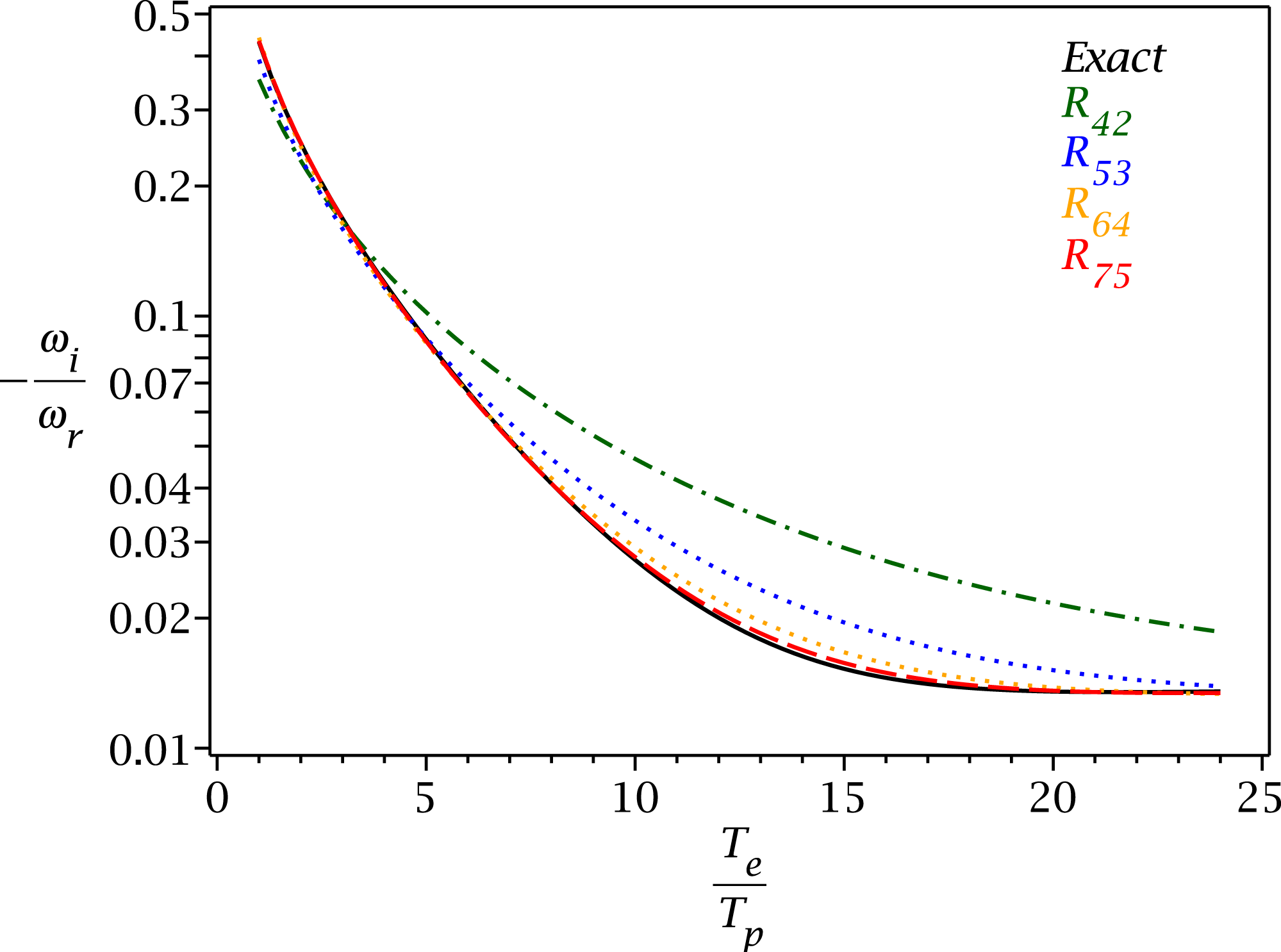
Figure 9. Landau damping of the ion-acoustic mode, calculated with exact
 $R(\unicode[STIX]{x1D701})$
– black line;
$R(\unicode[STIX]{x1D701})$
– black line;
 $R_{4,2}(\unicode[STIX]{x1D701})$
– green line;
$R_{4,2}(\unicode[STIX]{x1D701})$
– green line;
 $R_{5,3}(\unicode[STIX]{x1D701})$
- blue line;
$R_{5,3}(\unicode[STIX]{x1D701})$
- blue line;
 $R_{6,4}(\unicode[STIX]{x1D701})$
– orange line; and
$R_{6,4}(\unicode[STIX]{x1D701})$
– orange line; and
 $R_{7,5}(\unicode[STIX]{x1D701})$
– red line. The solutions represent the most precise dynamic closures that can be constructed for the third-order moment (heat flux), fourth-order moment, fifth-order moment and sixth-order moment. It was analytically verified that all closures are ‘reliable’, i.e. equivalent to the kinetic dispersion relation once
$R_{7,5}(\unicode[STIX]{x1D701})$
– red line. The solutions represent the most precise dynamic closures that can be constructed for the third-order moment (heat flux), fourth-order moment, fifth-order moment and sixth-order moment. It was analytically verified that all closures are ‘reliable’, i.e. equivalent to the kinetic dispersion relation once
 $R(\unicode[STIX]{x1D701})$
is replaced by the associated
$R(\unicode[STIX]{x1D701})$
is replaced by the associated
 $R_{n,n^{\prime }}(\unicode[STIX]{x1D701})$
approximant. The next most precise closure constructed for the seventh-order moment is
$R_{n,n^{\prime }}(\unicode[STIX]{x1D701})$
approximant. The next most precise closure constructed for the seventh-order moment is
 $R_{8,6}(\unicode[STIX]{x1D701})$
, which is not plotted, but we checked that the solution is basically not distinguishable (by eye) from the exact
$R_{8,6}(\unicode[STIX]{x1D701})$
, which is not plotted, but we checked that the solution is basically not distinguishable (by eye) from the exact
 $R(\unicode[STIX]{x1D701})$
solution. The figure shows that it is possible to reproduce Landau damping in the fluid framework to any desired precision.
$R(\unicode[STIX]{x1D701})$
solution. The figure shows that it is possible to reproduce Landau damping in the fluid framework to any desired precision.
3.17 Selected closures for the sixth-order moment
The sixth-order moment
 $X_{6}=m\int (v-u)^{6}f\,\text{d}v$
is linearized simply as
$X_{6}=m\int (v-u)^{6}f\,\text{d}v$
is linearized simply as
 $X_{6}^{(1)}=m\int v^{6}f^{(1)}\,\text{d}v$
, and since
$X_{6}^{(1)}=m\int v^{6}f^{(1)}\,\text{d}v$
, and since
 $$\begin{eqnarray}\frac{1}{\sqrt{\unicode[STIX]{x03C0}}}\int \frac{x^{6}e^{-x^{2}}}{x-x_{0}}\,\text{d}x=\text{sign}(k_{\Vert })\left(\frac{3}{4}\unicode[STIX]{x1D701}+\frac{1}{2}\unicode[STIX]{x1D701}^{3}+\unicode[STIX]{x1D701}^{5}R(\unicode[STIX]{x1D701})\right),\end{eqnarray}$$
and direct calculation yields
 $$\begin{eqnarray}X_{6}^{(1)}=-q_{r}\unicode[STIX]{x1D6F7}n_{0}\frac{p_{0}^{2}}{\unicode[STIX]{x1D70C}_{0}^{2}}\left(15+6\unicode[STIX]{x1D701}^{2}+4\unicode[STIX]{x1D701}^{4}+8\unicode[STIX]{x1D701}^{6}R(\unicode[STIX]{x1D701})\right),\end{eqnarray}$$
and alternatively
 $p_{0}/\unicode[STIX]{x1D70C}_{0}=v_{\text{th}}^{2}/2$
. Separating the deviation of this moment with tilde (similarly to
$p_{0}/\unicode[STIX]{x1D70C}_{0}=v_{\text{th}}^{2}/2$
. Separating the deviation of this moment with tilde (similarly to
 $\widetilde{r}$
, see also Part 1 of this guide) is done according to
$\widetilde{r}$
, see also Part 1 of this guide) is done according to
 $$\begin{eqnarray}\widetilde{X}_{6}^{(1)}=X_{6}^{(1)}-15\frac{p_{0}^{3}}{\unicode[STIX]{x1D70C}_{0}^{2}}\left(3\frac{p^{(1)}}{p_{0}}-2\frac{n^{(1)}}{n_{0}}\right),\end{eqnarray}$$
which directly yields
 $$\begin{eqnarray}\widetilde{X}_{6}^{(1)}=-q_{r}\unicode[STIX]{x1D6F7}n_{0}\frac{p_{0}^{2}}{\unicode[STIX]{x1D70C}_{0}^{2}}\left(30R(\unicode[STIX]{x1D701})-30+6\unicode[STIX]{x1D701}^{2}-90\unicode[STIX]{x1D701}^{2}R(\unicode[STIX]{x1D701})+4\unicode[STIX]{x1D701}^{4}+8\unicode[STIX]{x1D701}^{6}R(\unicode[STIX]{x1D701})\right).\end{eqnarray}$$
Considering static closures, the most precise power-series closure is constructed with
 $R_{6,4}(\unicode[STIX]{x1D701})$
and the closure reads
$R_{6,4}(\unicode[STIX]{x1D701})$
and the closure reads
 $$\begin{eqnarray}\displaystyle R_{6,4}(\unicode[STIX]{x1D701}):\quad \widetilde{X}_{6}^{(1)} & = & \displaystyle -\frac{3(180\unicode[STIX]{x03C0}^{2}-1197\unicode[STIX]{x03C0}+1984)\sqrt{\unicode[STIX]{x03C0}}}{(801\unicode[STIX]{x03C0}^{2}-5124\unicode[STIX]{x03C0}+8192)}v_{\text{th}}{\mathcal{H}}X_{5}^{(1)}\nonumber\\ \displaystyle & & \displaystyle +\,\frac{3(675\unicode[STIX]{x03C0}^{2}-4728\unicode[STIX]{x03C0}+8192)}{2(801\unicode[STIX]{x03C0}^{2}-5124\unicode[STIX]{x03C0}+8192)}v_{\text{th}}^{2}\widetilde{r}^{(1)}\nonumber\\ \displaystyle & & \displaystyle -\,\frac{3(285\unicode[STIX]{x03C0}-896)\sqrt{\unicode[STIX]{x03C0}}}{2(801\unicode[STIX]{x03C0}^{2}-5124\unicode[STIX]{x03C0}+8192)}v_{\text{th}}^{3}{\mathcal{H}}q^{(1)}\nonumber\\ \displaystyle & & \displaystyle -\,\frac{3(7065\unicode[STIX]{x03C0}^{2}-43056\unicode[STIX]{x03C0}+65536)}{4(801\unicode[STIX]{x03C0}^{2}-5124\unicode[STIX]{x03C0}+8192)}n_{0}v_{\text{th}}^{4}T^{(1)}\nonumber\\ \displaystyle & & \displaystyle -\,\frac{9(450\unicode[STIX]{x03C0}^{2}-2799\unicode[STIX]{x03C0}+4352)\sqrt{\unicode[STIX]{x03C0}}}{(801\unicode[STIX]{x03C0}^{2}-5124\unicode[STIX]{x03C0}+8192)}n_{0}T_{0}v_{\text{th}}^{3}{\mathcal{H}}u^{(1)}.\end{eqnarray}$$
This verifies that the dynamic
 $R_{6,4}(\unicode[STIX]{x1D701})$
closure (3.413) was calculated correctly, since from the simple fluid approach (Part 1), the static and dynamics closures (3.418), (3.413) must be related by
$R_{6,4}(\unicode[STIX]{x1D701})$
closure (3.413) was calculated correctly, since from the simple fluid approach (Part 1), the static and dynamics closures (3.418), (3.413) must be related by
 $$\begin{eqnarray}\frac{\unicode[STIX]{x2202}}{\unicode[STIX]{x2202}t}X_{5}^{(1)}+\unicode[STIX]{x2202}_{z}\widetilde{X}_{6}^{(1)}+\frac{15}{2}n_{0}v_{\text{th}}^{4}\unicode[STIX]{x2202}_{z}T^{(1)}=0.\end{eqnarray}$$
The most precise (power-series) dynamic closure for
 $\widetilde{X}_{6}^{(1)}$
can be constructed with approximant
$\widetilde{X}_{6}^{(1)}$
can be constructed with approximant
 $R_{7,5}(\unicode[STIX]{x1D701})$
, by searching for a solution
$R_{7,5}(\unicode[STIX]{x1D701})$
, by searching for a solution
 $$\begin{eqnarray}[\unicode[STIX]{x1D701}+\unicode[STIX]{x1D6FC}_{x_{6}}]\widetilde{X}_{6}^{(1)}=\unicode[STIX]{x1D6FC}_{x_{5}}X_{5}^{(1)}+\unicode[STIX]{x1D6FC}_{r}\widetilde{r}^{(1)}+\unicode[STIX]{x1D6FC}_{q}q^{(1)}+\unicode[STIX]{x1D6FC}_{t}T^{(1)}+\unicode[STIX]{x1D6FC}_{u}u^{(1)},\end{eqnarray}$$
and the closure in real space reads
 $$\begin{eqnarray}\displaystyle & \displaystyle R_{7,5}(\unicode[STIX]{x1D701}):\quad \left[\frac{\text{d}}{\text{d}t}+\frac{18(1545\unicode[STIX]{x03C0}^{2}-9743\unicode[STIX]{x03C0}+15360)\sqrt{\unicode[STIX]{x03C0}}}{(10800\unicode[STIX]{x03C0}^{3}-120915\unicode[STIX]{x03C0}^{2}+440160\unicode[STIX]{x03C0}-524288)}v_{\text{th}}\unicode[STIX]{x2202}_{z}{\mathcal{H}}\right]\widetilde{X}_{6}^{(1)} & \displaystyle \nonumber\\ \displaystyle & \displaystyle \quad \quad =+\,\frac{3(52425\unicode[STIX]{x03C0}^{2}-331584\unicode[STIX]{x03C0}+524288)}{2(10800\unicode[STIX]{x03C0}^{3}-120915\unicode[STIX]{x03C0}^{2}+440160\unicode[STIX]{x03C0}-524288)}v_{\text{th}}^{2}\unicode[STIX]{x2202}_{z}X_{5}^{(1)} & \displaystyle \nonumber\\ \displaystyle & \displaystyle \qquad \quad +\frac{3(7875\unicode[STIX]{x03C0}^{2}-50490\unicode[STIX]{x03C0}+80896)\sqrt{\unicode[STIX]{x03C0}}}{(10800\unicode[STIX]{x03C0}^{3}-120915\unicode[STIX]{x03C0}^{2}+440160\unicode[STIX]{x03C0}-524288)}v_{\text{th}}^{3}\unicode[STIX]{x2202}_{z}{\mathcal{H}}\widetilde{r}^{(1)} & \displaystyle \nonumber\\ \displaystyle & \displaystyle \qquad \quad +\frac{3(162000\unicode[STIX]{x03C0}^{3}-1758825\unicode[STIX]{x03C0}^{2}+6263040\unicode[STIX]{x03C0}-7340032)}{4(10800\unicode[STIX]{x03C0}^{3}-120915\unicode[STIX]{x03C0}^{2}+440160\unicode[STIX]{x03C0}-524288)}v_{\text{th}}^{4}\unicode[STIX]{x2202}_{z}q^{(1)} & \displaystyle \nonumber\\ \displaystyle & \displaystyle \qquad \quad -\frac{27(15825\unicode[STIX]{x03C0}^{2}-99260\unicode[STIX]{x03C0}+155648)\sqrt{\unicode[STIX]{x03C0}}}{2(10800\unicode[STIX]{x03C0}^{3}-120915\unicode[STIX]{x03C0}^{2}+440160\unicode[STIX]{x03C0}-524288)}v_{\text{th}}^{5}n_{0}\unicode[STIX]{x2202}_{z}{\mathcal{H}}T^{(1)} & \displaystyle \nonumber\\ \displaystyle & \displaystyle \qquad \quad +\frac{3(189000\unicode[STIX]{x03C0}^{3}-1612215\unicode[STIX]{x03C0}^{2}+4534656\unicode[STIX]{x03C0}-4194304)}{2(10800\unicode[STIX]{x03C0}^{3}-120915\unicode[STIX]{x03C0}^{2}+440160\unicode[STIX]{x03C0}-524288)}v_{\text{th}}^{4}n_{0}T_{0}\unicode[STIX]{x2202}_{z}u^{(1)}. & \displaystyle\end{eqnarray}$$
The closure has precision
 $o(\unicode[STIX]{x1D701}^{6})$
,
$o(\unicode[STIX]{x1D701}^{6})$
,
 $o(\unicode[STIX]{x1D701}^{-7})$
, and it was verified that the closure is reliable. The closure is plotted in figure 9 with the red line.
$o(\unicode[STIX]{x1D701}^{-7})$
, and it was verified that the closure is reliable. The closure is plotted in figure 9 with the red line.
3.18 Convergence of fluid and kinetic descriptions
In general, for a given
 $X_{n}$
, the most precise (power-series) closures are of course dynamic closures, and we have seen that for the third-order moment it is
$X_{n}$
, the most precise (power-series) closures are of course dynamic closures, and we have seen that for the third-order moment it is
 $R_{4,2}(\unicode[STIX]{x1D701})$
, for the fourth-order moment it is
$R_{4,2}(\unicode[STIX]{x1D701})$
, for the fourth-order moment it is
 $R_{5,3}(\unicode[STIX]{x1D701})$
, for the fifth-order moment it is
$R_{5,3}(\unicode[STIX]{x1D701})$
, for the fifth-order moment it is
 $R_{6,4}(\unicode[STIX]{x1D701})$
and for the sixth-order moment it is
$R_{6,4}(\unicode[STIX]{x1D701})$
and for the sixth-order moment it is
 $R_{7,5}(\unicode[STIX]{x1D701})$
. Therefore, it is reasonable to make a conjecture that for an
$R_{7,5}(\unicode[STIX]{x1D701})$
. Therefore, it is reasonable to make a conjecture that for an
 $n$
th-order moment
$n$
th-order moment
 $X_{n}$
, the most precise closure will be constructed with approximant
$X_{n}$
, the most precise closure will be constructed with approximant
 $R_{n+1,n-1}(\unicode[STIX]{x1D701})$
.
$R_{n+1,n-1}(\unicode[STIX]{x1D701})$
.
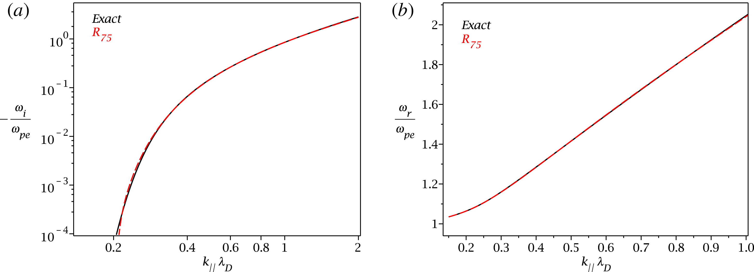
Figure 10. Landau damping of the Langmuir mode (a), and real frequency (b), calculated with the exact
 $R(\unicode[STIX]{x1D701})$
– black line, and
$R(\unicode[STIX]{x1D701})$
– black line, and
 $R_{7,5}(\unicode[STIX]{x1D701})$
– red line.
$R_{7,5}(\unicode[STIX]{x1D701})$
– red line.
The dynamic closures above are directly related to the most precise (power-series) static closures that can be constructed, and we have seen that for the third-order moment it is with approximant
 $R_{3,1}(\unicode[STIX]{x1D701})$
, for the fourth-order moment it is
$R_{3,1}(\unicode[STIX]{x1D701})$
, for the fourth-order moment it is
 $R_{4,2}(\unicode[STIX]{x1D701})$
, for the fifth-order moment it is
$R_{4,2}(\unicode[STIX]{x1D701})$
, for the fifth-order moment it is
 $R_{5,3}(\unicode[STIX]{x1D701})$
and for the sixth-order moment it is
$R_{5,3}(\unicode[STIX]{x1D701})$
and for the sixth-order moment it is
 $R_{6,4}(\unicode[STIX]{x1D701})$
, and therefore for an
$R_{6,4}(\unicode[STIX]{x1D701})$
, and therefore for an
 $n$
th-order moment, it will be with approximant
$n$
th-order moment, it will be with approximant
 $R_{n,n-2}(\unicode[STIX]{x1D701})$
. Regardless if dynamic or static closures are used, this implies that one can reproduce the (linear) Landau damping phenomenon in the fluid framework, to any desired precision, which establishes convergence of fluid and kinetic descriptions.
$R_{n,n-2}(\unicode[STIX]{x1D701})$
. Regardless if dynamic or static closures are used, this implies that one can reproduce the (linear) Landau damping phenomenon in the fluid framework, to any desired precision, which establishes convergence of fluid and kinetic descriptions.
The convergence was shown here in a 1-D (electrostatic) geometry, by considering the long-wavelength low-frequency ion-acoustic mode. Nevertheless, the 1-D closures have general validity, and are of course valid also for the Langmuir mode, that we considered in § 3.14. However, see the discussion about the limitations of the Langmuir mode modelling at the end of that section, since the closures can become unstable for
 $k_{\Vert }\unicode[STIX]{x1D706}_{D}<0.2$
, i.e. in the long-wavelength limit. For a curious reader, the damping and real frequencies of the Langmuir mode obtained with
$k_{\Vert }\unicode[STIX]{x1D706}_{D}<0.2$
, i.e. in the long-wavelength limit. For a curious reader, the damping and real frequencies of the Langmuir mode obtained with
 $R_{7,5}(\unicode[STIX]{x1D701})$
, are plotted in figure 10.
$R_{7,5}(\unicode[STIX]{x1D701})$
, are plotted in figure 10.
If one wants to pursue a proof of our conjecture, the general Landau integral with
 $x^{n}$
can be calculated, for example by considering separate cases for ‘
$x^{n}$
can be calculated, for example by considering separate cases for ‘
 $n$
’ being odd and even. The result can be expressed as
$n$
’ being odd and even. The result can be expressed as
 $$\begin{eqnarray}\displaystyle & & \displaystyle n=\text{odd}:\quad \frac{1}{\sqrt{\unicode[STIX]{x03C0}}}\int _{-\infty }^{\infty }\frac{x^{n}e^{-x^{2}}}{x-x_{0}}\,\text{d}x=\unicode[STIX]{x1D701}^{n-1}R(\unicode[STIX]{x1D701})+\mathop{\sum }_{l=0}^{(n-3)/2}\frac{(n-2l-2)!!}{2^{(n-2l-1)/2}}\unicode[STIX]{x1D701}^{2l};\nonumber\\ \displaystyle & & \displaystyle n=\text{even}:\quad \frac{1}{\sqrt{\unicode[STIX]{x03C0}}}\int _{-\infty }^{\infty }\frac{x^{n}e^{-x^{2}}}{x-x_{0}}\,\text{d}x=\text{sign}(k_{\Vert })\left[\unicode[STIX]{x1D701}^{n-1}R(\unicode[STIX]{x1D701})+\mathop{\sum }_{l=0}^{(n-4)/2}\frac{(n-2l-3)!!}{2^{(n-2l-2)/2}}\unicode[STIX]{x1D701}^{2l+1}\right],\nonumber\\ \displaystyle & & \displaystyle\end{eqnarray}$$
and it is valid for
 $n\geqslant 3$
. Alternatively, one could say that the result is valid for
$n\geqslant 3$
. Alternatively, one could say that the result is valid for
 $n\geqslant 1$
and that the sums are zero when the upper index is negative. One can write expressions for the general
$n\geqslant 1$
and that the sums are zero when the upper index is negative. One can write expressions for the general
 $n$
th moment
$n$
th moment
 $X_{n}^{(1)}$
, and the moment is proportional to
$X_{n}^{(1)}$
, and the moment is proportional to
 $\unicode[STIX]{x1D701}^{n}R(\unicode[STIX]{x1D701})$
. Therefore, considering static closures where the
$\unicode[STIX]{x1D701}^{n}R(\unicode[STIX]{x1D701})$
. Therefore, considering static closures where the
 $X_{n}^{(1)}$
is expressed through all the lower-order moments
$X_{n}^{(1)}$
is expressed through all the lower-order moments
 $X_{m}^{(1)}$
;
$X_{m}^{(1)}$
;
 $m=1\ldots n-1$
(for even moments the deviations
$m=1\ldots n-1$
(for even moments the deviations
 $\widetilde{X}^{(1)}$
have to be considered), it is obvious that the closure has to be achieved with the
$\widetilde{X}^{(1)}$
have to be considered), it is obvious that the closure has to be achieved with the
 $n$
th-order Padé approximant of
$n$
th-order Padé approximant of
 $R(\unicode[STIX]{x1D701})$
. Similarly, considering dynamic closures where the
$R(\unicode[STIX]{x1D701})$
. Similarly, considering dynamic closures where the
 $\unicode[STIX]{x1D701}X_{n}^{(1)}\sim \unicode[STIX]{x1D701}^{n+1}R(\unicode[STIX]{x1D701})$
is expressed through all the lower-order moments, the closure has to be achieved with the
$\unicode[STIX]{x1D701}X_{n}^{(1)}\sim \unicode[STIX]{x1D701}^{n+1}R(\unicode[STIX]{x1D701})$
is expressed through all the lower-order moments, the closure has to be achieved with the
 $(n+1)$
th-order Padé approximant of
$(n+1)$
th-order Padé approximant of
 $R(\unicode[STIX]{x1D701})$
. To finish the proof, one needs to show that the number of required asymptotic points corresponds to
$R(\unicode[STIX]{x1D701})$
. To finish the proof, one needs to show that the number of required asymptotic points corresponds to
 $R_{n,n-2}(\unicode[STIX]{x1D701})$
and
$R_{n,n-2}(\unicode[STIX]{x1D701})$
and
 $R_{n+1,n-1}(\unicode[STIX]{x1D701})$
, and that such a closure is ‘reliable’.
$R_{n+1,n-1}(\unicode[STIX]{x1D701})$
, and that such a closure is ‘reliable’.
The next logical step would be to establish such analytic convergence of fluid and kinetic descriptions in a 3-D electromagnetic geometry in the gyrotropic limit. However, in three dimensions, for a given
 $n$
th-order tensor
$n$
th-order tensor
 $\unicode[STIX]{x1D653}_{n}$
, the number of its gyrotropic moments is equal to
$\unicode[STIX]{x1D653}_{n}$
, the number of its gyrotropic moments is equal to
 $1+\text{int}[n/2]$
and increases with
$1+\text{int}[n/2]$
and increases with
 $n$
. Therefore, it might be much more difficult to show the convergence in three dimensions, even though the convergence should still exist.
$n$
. Therefore, it might be much more difficult to show the convergence in three dimensions, even though the convergence should still exist.
4 Three-dimensional geometry (electromagnetic)
Considering gyrotropic
 $f_{0}$
, let us remind ourselves of the linearized Vlasov equation (2.12), that reads
$f_{0}$
, let us remind ourselves of the linearized Vlasov equation (2.12), that reads
 $$\begin{eqnarray}\frac{\unicode[STIX]{x2202}f^{(1)}}{\unicode[STIX]{x2202}t}+\boldsymbol{v}\boldsymbol{\cdot }\unicode[STIX]{x1D735}f^{(1)}-\frac{q_{r}B_{0}}{m_{r}c}\frac{\unicode[STIX]{x2202}f^{(1)}}{\unicode[STIX]{x2202}\unicode[STIX]{x1D719}}=-\frac{q_{r}}{m_{r}}\left(\boldsymbol{E}^{(1)}+\frac{1}{c}\boldsymbol{v}\times \boldsymbol{B}^{(1)}\right)\boldsymbol{\cdot }\unicode[STIX]{x1D735}_{v}\,f_{0}.\end{eqnarray}$$
We want to describe the simplest kinetic effects and we demand that
 $f^{(1)}$
must be gyrotropic as well, so
$f^{(1)}$
must be gyrotropic as well, so
 $\unicode[STIX]{x2202}f^{(1)}/\unicode[STIX]{x2202}\unicode[STIX]{x1D719}=0$
. This eliminates the third term on the left-hand side of (4.1) that is responsible for complicated non-gyrotropic effects with associated Bessel functions. However, even without this term the equation still appears to be complicated. For gyrotropic
$\unicode[STIX]{x2202}f^{(1)}/\unicode[STIX]{x2202}\unicode[STIX]{x1D719}=0$
. This eliminates the third term on the left-hand side of (4.1) that is responsible for complicated non-gyrotropic effects with associated Bessel functions. However, even without this term the equation still appears to be complicated. For gyrotropic
 $f_{0}$
, the operator on the right-hand side can be shown to be (see B, equation (B 9), written in Fourier space)
$f_{0}$
, the operator on the right-hand side can be shown to be (see B, equation (B 9), written in Fourier space)
 $$\begin{eqnarray}\displaystyle \left(\boldsymbol{E}+\frac{1}{c}\boldsymbol{v}\times \boldsymbol{B}\right)\boldsymbol{\cdot }\unicode[STIX]{x1D735}_{v}f_{0} & = & \displaystyle (E_{x}v_{x}+E_{y}v_{y})\left[\left(1-\frac{v_{\Vert }k_{\Vert }}{\unicode[STIX]{x1D714}}\right)\frac{1}{v_{\bot }}\frac{\unicode[STIX]{x2202}f_{0}}{\unicode[STIX]{x2202}v_{\bot }}+\frac{k_{\Vert }}{\unicode[STIX]{x1D714}}\frac{\unicode[STIX]{x2202}f_{0}}{\unicode[STIX]{x2202}v_{\Vert }}\right]\nonumber\\ \displaystyle & & \displaystyle +\,E_{z}\left[\frac{\unicode[STIX]{x2202}f_{0}}{\unicode[STIX]{x2202}v_{\Vert }}-\frac{v_{x}k_{x}+v_{y}k_{y}}{\unicode[STIX]{x1D714}}\left(\frac{\unicode[STIX]{x2202}f_{0}}{\unicode[STIX]{x2202}v_{\Vert }}-\frac{v_{\Vert }}{v_{\bot }}\frac{\unicode[STIX]{x2202}f_{0}}{\unicode[STIX]{x2202}v_{\bot }}\right)\right].\end{eqnarray}$$
Written in the cylindrical coordinate system
 $$\begin{eqnarray}\displaystyle \boldsymbol{v}=\left(\begin{array}{@{}c@{}}v_{\bot }\cos \unicode[STIX]{x1D719}\\ v_{\bot }\sin \unicode[STIX]{x1D719}\\ v_{\Vert }\end{array}\right),\quad \boldsymbol{k}=\left(\begin{array}{@{}c@{}}k_{\bot }\cos \unicode[STIX]{x1D713}\\ k_{\bot }\sin \unicode[STIX]{x1D713}\\ k_{\Vert }\end{array}\right), & & \displaystyle\end{eqnarray}$$
so that
 $$\begin{eqnarray}\displaystyle & \displaystyle v_{x}k_{x}+v_{y}k_{y}=v_{\bot }k_{\bot }\cos \unicode[STIX]{x1D719}\cos \unicode[STIX]{x1D713}+v_{\bot }k_{\bot }\sin \unicode[STIX]{x1D719}\sin \unicode[STIX]{x1D713}=v_{\bot }k_{\bot }\cos (\unicode[STIX]{x1D719}-\unicode[STIX]{x1D713}); & \displaystyle\end{eqnarray}$$
 $$\begin{eqnarray}\displaystyle & \displaystyle \boldsymbol{v}\boldsymbol{\cdot }\boldsymbol{k}=v_{\Vert }k_{\Vert }+v_{\bot }k_{\bot }\cos (\unicode[STIX]{x1D719}-\unicode[STIX]{x1D713}), & \displaystyle\end{eqnarray}$$
which yields
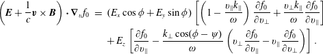 $$\begin{eqnarray}\displaystyle \left(\boldsymbol{E}+\frac{1}{c}\boldsymbol{v}\times \boldsymbol{B}\right)\boldsymbol{\cdot }\unicode[STIX]{x1D735}_{v}f_{0} & = & \displaystyle (E_{x}\cos \unicode[STIX]{x1D719}+E_{y}\sin \unicode[STIX]{x1D719})\left[\left(1-\frac{v_{\Vert }k_{\Vert }}{\unicode[STIX]{x1D714}}\right)\frac{\unicode[STIX]{x2202}f_{0}}{\unicode[STIX]{x2202}v_{\bot }}+\frac{v_{\bot }k_{\Vert }}{\unicode[STIX]{x1D714}}\frac{\unicode[STIX]{x2202}f_{0}}{\unicode[STIX]{x2202}v_{\Vert }}\right]\nonumber\\ \displaystyle & & \displaystyle +\,E_{z}\left[\frac{\unicode[STIX]{x2202}f_{0}}{\unicode[STIX]{x2202}v_{\Vert }}-\frac{k_{\bot }\cos (\unicode[STIX]{x1D719}-\unicode[STIX]{x1D713})}{\unicode[STIX]{x1D714}}\left(v_{\bot }\frac{\unicode[STIX]{x2202}f_{0}}{\unicode[STIX]{x2202}v_{\Vert }}-v_{\Vert }\frac{\unicode[STIX]{x2202}f_{0}}{\unicode[STIX]{x2202}v_{\bot }}\right)\right].\end{eqnarray}$$
The Vlasov equation in Fourier space now reads
 $$\begin{eqnarray}\displaystyle & & \displaystyle -i\left(\unicode[STIX]{x1D714}-v_{\Vert }k_{\Vert }-v_{\bot }k_{\bot }\cos (\unicode[STIX]{x1D719}-\unicode[STIX]{x1D713})\right)f^{(1)}\nonumber\\ \displaystyle & & \displaystyle \quad =-\frac{q_{r}}{m_{r}}\left\{(E_{x}\cos \unicode[STIX]{x1D719}+E_{y}\sin \unicode[STIX]{x1D719})\left[\left(1-\frac{v_{\Vert }k_{\Vert }}{\unicode[STIX]{x1D714}}\right)\frac{\unicode[STIX]{x2202}f_{0}}{\unicode[STIX]{x2202}v_{\bot }}+\frac{v_{\bot }k_{\Vert }}{\unicode[STIX]{x1D714}}\frac{\unicode[STIX]{x2202}f_{0}}{\unicode[STIX]{x2202}v_{\Vert }}\right]\right.\nonumber\\ \displaystyle & & \displaystyle \qquad \left.+\,E_{z}\left[\frac{\unicode[STIX]{x2202}f_{0}}{\unicode[STIX]{x2202}v_{\Vert }}-\frac{k_{\bot }\cos (\unicode[STIX]{x1D719}-\unicode[STIX]{x1D713})}{\unicode[STIX]{x1D714}}\left(v_{\bot }\frac{\unicode[STIX]{x2202}f_{0}}{\unicode[STIX]{x2202}v_{\Vert }}-v_{\Vert }\frac{\unicode[STIX]{x2202}f_{0}}{\unicode[STIX]{x2202}v_{\bot }}\right)\right]\right\}.\end{eqnarray}$$
This equation is not very useful. If the equation is divided by
 $(\unicode[STIX]{x1D714}-\boldsymbol{v}\boldsymbol{\cdot }\boldsymbol{k})$
to obtain
$(\unicode[STIX]{x1D714}-\boldsymbol{v}\boldsymbol{\cdot }\boldsymbol{k})$
to obtain
 $f^{(1)}$
, and integration over
$f^{(1)}$
, and integration over
 $\int _{0}^{2\unicode[STIX]{x03C0}}\,\text{d}\unicode[STIX]{x1D719}$
is attempted, this leads to integrals that are not well defined. On the other hand, if (4.7) is directly integrated over
$\int _{0}^{2\unicode[STIX]{x03C0}}\,\text{d}\unicode[STIX]{x1D719}$
is attempted, this leads to integrals that are not well defined. On the other hand, if (4.7) is directly integrated over
 $\text{d}\unicode[STIX]{x1D719}$
(each side separately), almost all the terms disappear since
$\text{d}\unicode[STIX]{x1D719}$
(each side separately), almost all the terms disappear since
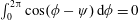 $\int _{0}^{2\unicode[STIX]{x03C0}}\cos (\unicode[STIX]{x1D719}-\unicode[STIX]{x1D713})\,\text{d}\unicode[STIX]{x1D719}=0$
etc., except
$\int _{0}^{2\unicode[STIX]{x03C0}}\cos (\unicode[STIX]{x1D719}-\unicode[STIX]{x1D713})\,\text{d}\unicode[STIX]{x1D719}=0$
etc., except
 $$\begin{eqnarray}-i\left(\unicode[STIX]{x1D714}-v_{\Vert }k_{\Vert }\right)f^{(1)}=-\frac{q_{r}}{m_{r}}E_{z}\frac{\unicode[STIX]{x2202}f_{0}}{\unicode[STIX]{x2202}v_{\Vert }},\end{eqnarray}$$
and the system reduces to the simplest case of Landau damping that we have already described in detail (even though only in a 1-D geometry). We could divide (4.8) by
 $(\unicode[STIX]{x1D714}-v_{\Vert }k_{\Vert })$
, integrate the system in a 3-D geometry and consider Landau fluid closures, but this would be a bit boring right now. We want to get a few more kinetic effects out of the system. We need a different approach and we need to obtain a better gyrotropic limit for
$(\unicode[STIX]{x1D714}-v_{\Vert }k_{\Vert })$
, integrate the system in a 3-D geometry and consider Landau fluid closures, but this would be a bit boring right now. We want to get a few more kinetic effects out of the system. We need a different approach and we need to obtain a better gyrotropic limit for
 $f^{(1)}$
.
$f^{(1)}$
.
It turns out that to obtain the correct gyrotropic limit for
 $f^{(1)}$
, the third term in the Vlasov equation (4.1) cannot just be straightforwardly neglected. The term has to be kept there, the relatively complicated integration around the unperturbed orbit has to be performed (see appendix C), and only then can the term be removed in a limit. This is very similar to other mathematical techniques that were encountered earlier, for example when calculating the Fourier transform of
$f^{(1)}$
, the third term in the Vlasov equation (4.1) cannot just be straightforwardly neglected. The term has to be kept there, the relatively complicated integration around the unperturbed orbit has to be performed (see appendix C), and only then can the term be removed in a limit. This is very similar to other mathematical techniques that were encountered earlier, for example when calculating the Fourier transform of
 $\text{sign}(k_{\Vert })$
, where instead of that function, one needs to consider
$\text{sign}(k_{\Vert })$
, where instead of that function, one needs to consider
 $\text{sign}(k_{\Vert })e^{-\unicode[STIX]{x1D6FC}|k_{\Vert }|}$
, and only after the calculation is the term removed with the limit
$\text{sign}(k_{\Vert })e^{-\unicode[STIX]{x1D6FC}|k_{\Vert }|}$
, and only after the calculation is the term removed with the limit
 $\unicode[STIX]{x1D6FC}\rightarrow 0$
. Without the additional term
$\unicode[STIX]{x1D6FC}\rightarrow 0$
. Without the additional term
 $e^{-\unicode[STIX]{x1D6FC}|k_{\Vert }|}$
that was removed later, the calculations were not clearly defined, and a very similar situation is encountered now. Nevertheless, it is indeed mind boggling that the complicated integration around the unperturbed orbit has to be performed to recover the gyrotropic limit. This is exactly why the 3-D case is so much more complicated than the previously studied 1-D case, even though the Landau fluid closures will not be more complicated at all, as we will see later. An alternative approach that we will discuss only very briefly, is to use the guiding-centre variables where the gyrotropic limit is recovered perhaps more naturally. However, we will skip a huge amount of calculations that lead to the guiding-centre approach, so the amount of complexity is probably similar in the end.
$e^{-\unicode[STIX]{x1D6FC}|k_{\Vert }|}$
that was removed later, the calculations were not clearly defined, and a very similar situation is encountered now. Nevertheless, it is indeed mind boggling that the complicated integration around the unperturbed orbit has to be performed to recover the gyrotropic limit. This is exactly why the 3-D case is so much more complicated than the previously studied 1-D case, even though the Landau fluid closures will not be more complicated at all, as we will see later. An alternative approach that we will discuss only very briefly, is to use the guiding-centre variables where the gyrotropic limit is recovered perhaps more naturally. However, we will skip a huge amount of calculations that lead to the guiding-centre approach, so the amount of complexity is probably similar in the end.
4.1 Gyrotropic limit for
$f^{(1)}$

We need to consider the full kinetic
 $f^{(1)}$
with all non-gyrotropic effects, that is obtained in appendix C, equation (C 47). By using the
$f^{(1)}$
with all non-gyrotropic effects, that is obtained in appendix C, equation (C 47). By using the
 $z$
-component of the induction equation
$z$
-component of the induction equation
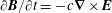 $\unicode[STIX]{x2202}\boldsymbol{B}/\unicode[STIX]{x2202}t=-c\unicode[STIX]{x1D735}\times \boldsymbol{E}$
written in Fourier space (C 71) (that is an equation of general validity not introducing any simplifications), the general
$\unicode[STIX]{x2202}\boldsymbol{B}/\unicode[STIX]{x2202}t=-c\unicode[STIX]{x1D735}\times \boldsymbol{E}$
written in Fourier space (C 71) (that is an equation of general validity not introducing any simplifications), the general
 $f^{(1)}$
(C 47) is slightly rewritten as
$f^{(1)}$
(C 47) is slightly rewritten as
 $$\begin{eqnarray}\displaystyle f_{r}^{(1)} & = & \displaystyle -\frac{iq_{r}}{m_{r}}\mathop{\sum }_{n=-\infty }^{\infty }\mathop{\sum }_{m=-\infty }^{\infty }\frac{e^{+i(m-n)(\unicode[STIX]{x1D719}-\unicode[STIX]{x1D713})}}{\unicode[STIX]{x1D714}-k_{\Vert }v_{\Vert }-n\unicode[STIX]{x1D6FA}_{r}}\text{J}_{m}(\unicode[STIX]{x1D706}_{r})\left\{\left[\frac{n\text{J}_{n}(\unicode[STIX]{x1D706}_{r})}{\unicode[STIX]{x1D706}_{r}}\left(E_{x}\cos \unicode[STIX]{x1D713}+E_{y}\sin \unicode[STIX]{x1D713}\right)\right.\right.\nonumber\\ \displaystyle & & \displaystyle \left.+\,i\text{J}_{n}^{\prime }(\unicode[STIX]{x1D706}_{r})\frac{\unicode[STIX]{x1D714}}{ck_{\bot }}B_{z}\right]\left[\left(1-\frac{k_{\Vert }v_{\Vert }}{\unicode[STIX]{x1D714}}\right)\frac{\unicode[STIX]{x2202}f_{0r}}{\unicode[STIX]{x2202}v_{\bot }}+\frac{k_{\Vert }v_{\bot }}{\unicode[STIX]{x1D714}}\frac{\unicode[STIX]{x2202}f_{0r}}{\unicode[STIX]{x2202}v_{\Vert }}\right]\nonumber\\ \displaystyle & & \displaystyle \left.+\,E_{z}\text{J}_{n}(\unicode[STIX]{x1D706}_{r})\left[\frac{\unicode[STIX]{x2202}f_{0r}}{\unicode[STIX]{x2202}v_{\Vert }}-\frac{n\unicode[STIX]{x1D6FA}_{r}}{\unicode[STIX]{x1D714}}\left(\frac{\unicode[STIX]{x2202}f_{0r}}{\unicode[STIX]{x2202}v_{\Vert }}-\frac{v_{\Vert }}{v_{\bot }}\frac{\unicode[STIX]{x2202}f_{0r}}{\unicode[STIX]{x2202}v_{\bot }}\right)\right]\right\}.\end{eqnarray}$$
This
 $f^{(1)}$
contains all the information of linear kinetic theory, with associated Bessel functions
$f^{(1)}$
contains all the information of linear kinetic theory, with associated Bessel functions
 $\text{J}_{n}(\unicode[STIX]{x1D706}_{r})$
, where
$\text{J}_{n}(\unicode[STIX]{x1D706}_{r})$
, where
 $\unicode[STIX]{x1D706}_{r}=k_{\bot }v_{\bot }/\unicode[STIX]{x1D6FA}_{r}$
and
$\unicode[STIX]{x1D706}_{r}=k_{\bot }v_{\bot }/\unicode[STIX]{x1D6FA}_{r}$
and
 $\unicode[STIX]{x1D6FA}_{r}=q_{r}B_{0}/(m_{r}c)$
. Two summations through integers ‘
$\unicode[STIX]{x1D6FA}_{r}=q_{r}B_{0}/(m_{r}c)$
. Two summations through integers ‘
 $n$
’ and ‘
$n$
’ and ‘
 $m$
’ are present in (4.9), that originate from using identities (C 10), (C 11). The general (4.9) contains ‘singularities’ where
$m$
’ are present in (4.9), that originate from using identities (C 10), (C 11). The general (4.9) contains ‘singularities’ where
 $\unicode[STIX]{x1D714}-k_{\Vert }v_{\Vert }-n\unicode[STIX]{x1D6FA}_{r}$
becomes zero, that are called wave–particle resonances. For
$\unicode[STIX]{x1D714}-k_{\Vert }v_{\Vert }-n\unicode[STIX]{x1D6FA}_{r}$
becomes zero, that are called wave–particle resonances. For
 $n=0$
the resonance is called the Landau resonance, and resonances for
$n=0$
the resonance is called the Landau resonance, and resonances for
 $n\neq 0$
are called cyclotron resonances. To get rid of the summations and Bessel functions, we want to consider the dynamics at spatial scales that are much larger than the particle gyroradius, which corresponds to limit
$n\neq 0$
are called cyclotron resonances. To get rid of the summations and Bessel functions, we want to consider the dynamics at spatial scales that are much larger than the particle gyroradius, which corresponds to limit
 $\unicode[STIX]{x1D706}_{r}\ll 1$
. Additionally, we will need to consider low-frequency limit
$\unicode[STIX]{x1D706}_{r}\ll 1$
. Additionally, we will need to consider low-frequency limit
 $\unicode[STIX]{x1D714}/\unicode[STIX]{x1D6FA}_{r}\ll 1$
. We find it illuminating to first separate the
$\unicode[STIX]{x1D714}/\unicode[STIX]{x1D6FA}_{r}\ll 1$
. We find it illuminating to first separate the
 $n=0$
resonance from all the other expressions, without performing any approximations, i.e. we want to separate
$n=0$
resonance from all the other expressions, without performing any approximations, i.e. we want to separate
 $$\begin{eqnarray}f_{r}^{(1)}=f_{r}^{(1)}|_{n=0}+f_{r}^{(1)}|_{n\neq 0}.\end{eqnarray}$$
Separating the
 $n=0$
case directly yields
$n=0$
case directly yields
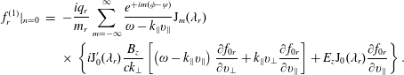 $$\begin{eqnarray}\displaystyle f_{r}^{(1)}|_{n=0} & = & \displaystyle -\frac{iq_{r}}{m_{r}}\mathop{\sum }_{m=-\infty }^{\infty }\frac{e^{+im(\unicode[STIX]{x1D719}-\unicode[STIX]{x1D713})}}{\unicode[STIX]{x1D714}-k_{\Vert }v_{\Vert }}\text{J}_{m}(\unicode[STIX]{x1D706}_{r})\nonumber\\ \displaystyle & & \displaystyle \times \,\left\{i\text{J}_{0}^{\prime }(\unicode[STIX]{x1D706}_{r})\frac{B_{z}}{ck_{\bot }}\left[\left(\unicode[STIX]{x1D714}-k_{\Vert }v_{\Vert }\right)\frac{\unicode[STIX]{x2202}f_{0r}}{\unicode[STIX]{x2202}v_{\bot }}+k_{\Vert }v_{\bot }\frac{\unicode[STIX]{x2202}f_{0r}}{\unicode[STIX]{x2202}v_{\Vert }}\right]+E_{z}\text{J}_{0}(\unicode[STIX]{x1D706}_{r})\frac{\unicode[STIX]{x2202}f_{0r}}{\unicode[STIX]{x2202}v_{\Vert }}\right\}.\end{eqnarray}$$
Note that
 $n\text{J}_{n}(x)/x=(\text{J}_{n-1}(x)+\text{J}_{n+1}(x))/2$
, which when evaluated for
$n\text{J}_{n}(x)/x=(\text{J}_{n-1}(x)+\text{J}_{n+1}(x))/2$
, which when evaluated for
 $n=0$
is zero exactly, since
$n=0$
is zero exactly, since
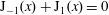 $\text{J}_{-1}(x)+\text{J}_{1}(x)=0$
exactly. Since there is no dependence on angles
$\text{J}_{-1}(x)+\text{J}_{1}(x)=0$
exactly. Since there is no dependence on angles
 $\unicode[STIX]{x1D719},\unicode[STIX]{x1D713}$
inside of the big brackets, the sum can be summed (or put to its original form where it came from)
$\unicode[STIX]{x1D719},\unicode[STIX]{x1D713}$
inside of the big brackets, the sum can be summed (or put to its original form where it came from)
 $$\begin{eqnarray}\displaystyle f_{r}^{(1)}|_{n=0} & = & \displaystyle -\frac{q_{r}}{m_{r}}\frac{e^{+i\unicode[STIX]{x1D706}_{r}\sin (\unicode[STIX]{x1D719}-\unicode[STIX]{x1D713})}}{\unicode[STIX]{x1D714}-k_{\Vert }v_{\Vert }}\left\{-\text{J}_{0}^{\prime }(\unicode[STIX]{x1D706}_{r})\frac{B_{z}}{ck_{\bot }}\left[\left(\unicode[STIX]{x1D714}-k_{\Vert }v_{\Vert }\right)\frac{\unicode[STIX]{x2202}f_{0r}}{\unicode[STIX]{x2202}v_{\bot }}+k_{\Vert }v_{\bot }\frac{\unicode[STIX]{x2202}f_{0r}}{\unicode[STIX]{x2202}v_{\Vert }}\right]\right.\nonumber\\ \displaystyle & & \displaystyle \left.+\,iE_{z}\text{J}_{0}(\unicode[STIX]{x1D706}_{r})\frac{\unicode[STIX]{x2202}f_{0r}}{\unicode[STIX]{x2202}v_{\Vert }}\right\}.\end{eqnarray}$$
Very interestingly, for one
 $B_{z}$
term, the complicated denominator
$B_{z}$
term, the complicated denominator
 $\unicode[STIX]{x1D714}-k_{\Vert }v_{\Vert }$
cancels out, yielding
$\unicode[STIX]{x1D714}-k_{\Vert }v_{\Vert }$
cancels out, yielding
 $$\begin{eqnarray}\displaystyle f_{r}^{(1)}|_{n=0} & = & \displaystyle -\frac{q_{r}}{m_{r}}e^{+i\unicode[STIX]{x1D706}_{r}\sin (\unicode[STIX]{x1D719}-\unicode[STIX]{x1D713})}\left\{-\text{J}_{0}^{\prime }(\unicode[STIX]{x1D706}_{r})\frac{B_{z}}{ck_{\bot }}\left[\frac{\unicode[STIX]{x2202}f_{0r}}{\unicode[STIX]{x2202}v_{\bot }}+\frac{k_{\Vert }v_{\bot }}{\unicode[STIX]{x1D714}-k_{\Vert }v_{\Vert }}\frac{\unicode[STIX]{x2202}f_{0r}}{\unicode[STIX]{x2202}v_{\Vert }}\right]\right.\nonumber\\ \displaystyle & & \displaystyle \left.+\,\text{J}_{0}(\unicode[STIX]{x1D706}_{r})\frac{iE_{z}}{\unicode[STIX]{x1D714}-k_{\Vert }v_{\Vert }}\frac{\unicode[STIX]{x2202}f_{0r}}{\unicode[STIX]{x2202}v_{\Vert }}\right\}.\end{eqnarray}$$
This is an exact kinetic expression for
 $f^{(1)}$
corresponding to
$f^{(1)}$
corresponding to
 $n=0$
resonances, that is accompanied by an expression for all the other resonances
$n=0$
resonances, that is accompanied by an expression for all the other resonances
 $f^{(1)}|_{n\neq 0}$
(that is equivalent to (4.9) where
$f^{(1)}|_{n\neq 0}$
(that is equivalent to (4.9) where
 $n\neq 0$
is added below the sum with
$n\neq 0$
is added below the sum with
 $n$
). Now considering the limit
$n$
). Now considering the limit
 $\unicode[STIX]{x1D706}_{r}\ll 1$
, the Bessel functions
$\unicode[STIX]{x1D706}_{r}\ll 1$
, the Bessel functions
 $\text{J}_{0}(\unicode[STIX]{x1D706}_{r})=1$
,
$\text{J}_{0}(\unicode[STIX]{x1D706}_{r})=1$
,
 $\text{J}_{0}^{\prime }(\unicode[STIX]{x1D706}_{r})=-\unicode[STIX]{x1D706}_{r}/2$
, the exponential term disappears, which yields the final
$\text{J}_{0}^{\prime }(\unicode[STIX]{x1D706}_{r})=-\unicode[STIX]{x1D706}_{r}/2$
, the exponential term disappears, which yields the final
 $f^{(1)}$
in the gyrotropic limit that reads
$f^{(1)}$
in the gyrotropic limit that reads
or alternatively
 $$\begin{eqnarray}f_{r}^{(1)}=\underbrace{-\frac{B_{z}}{2B_{0}}v_{\bot }\frac{\unicode[STIX]{x2202}f_{0r}}{\unicode[STIX]{x2202}v_{\bot }}}_{\unicode[STIX]{x1D707}=\text{const.}}\underbrace{-\frac{B_{z}}{2B_{0}}\frac{k_{\Vert }v_{\bot }^{2}}{(\unicode[STIX]{x1D714}-k_{\Vert }v_{\Vert })}\frac{\unicode[STIX]{x2202}f_{0r}}{\unicode[STIX]{x2202}v_{\Vert }}}_{\text{magnetic mirror force}}\underbrace{-\frac{q_{r}}{m_{r}}\frac{iE_{z}}{(\unicode[STIX]{x1D714}-k_{\Vert }v_{\Vert })}\frac{\unicode[STIX]{x2202}f_{0r}}{\unicode[STIX]{x2202}v_{\Vert }}}_{\text{Coulomb force}}.\end{eqnarray}$$
As we will see shortly in § 4.2, the expression has a very nice physical interpretation, where the first term comes from the conservation of the magnetic moment
 $\unicode[STIX]{x1D707}$
, the second term comes from the magnetic mirror force and the third term comes from the Coulomb force. The same expression is obtained by directly picking up the
$\unicode[STIX]{x1D707}$
, the second term comes from the magnetic mirror force and the third term comes from the Coulomb force. The same expression is obtained by directly picking up the
 $m=0$
,
$m=0$
,
 $n=0$
contributions from the general (4.9). Up to replacing
$n=0$
contributions from the general (4.9). Up to replacing
 $B_{z}$
with
$B_{z}$
with
 $|\boldsymbol{B}|$
, the expression agrees for example with (19) of Ferrière & André (Reference Ferrière and André2002), and is of course equivalent to expressions of Snyder et al. (Reference Snyder, Hammett and Dorland1997) (formulated in the gyrofluid formalism). In those works, the expression is derived perhaps more elegantly, in the so-called guiding-centre limit of the Vlasov equation (see Kulsrud Reference Kulsrud, Galeev and Sudan1983). The difference between
$|\boldsymbol{B}|$
, the expression agrees for example with (19) of Ferrière & André (Reference Ferrière and André2002), and is of course equivalent to expressions of Snyder et al. (Reference Snyder, Hammett and Dorland1997) (formulated in the gyrofluid formalism). In those works, the expression is derived perhaps more elegantly, in the so-called guiding-centre limit of the Vlasov equation (see Kulsrud Reference Kulsrud, Galeev and Sudan1983). The difference between
 $B_{z}$
and
$B_{z}$
and
 $|\boldsymbol{B}|$
arises, because the fully kinetic
$|\boldsymbol{B}|$
arises, because the fully kinetic
 $f^{(1)}$
in (4.9) is linearized completely.
$f^{(1)}$
in (4.9) is linearized completely.
Note that to obtain the gyrotropic limit (4.14), we did not have to explicitly perform the low-frequency limit
 $\unicode[STIX]{x1D714}/\unicode[STIX]{x1D6FA}_{r}\ll 1$
. However, it is important to emphasize that by only picking up the
$\unicode[STIX]{x1D714}/\unicode[STIX]{x1D6FA}_{r}\ll 1$
. However, it is important to emphasize that by only picking up the
 $n=0$
resonances, we have performed the low-frequency limit implicitly. The power-series expansion of the Bessel functions for
$n=0$
resonances, we have performed the low-frequency limit implicitly. The power-series expansion of the Bessel functions for
 $n\geqslant 0$
reads (with integer
$n\geqslant 0$
reads (with integer
 $n$
)
$n$
)
 $$\begin{eqnarray}\text{J}_{n}(x)=\mathop{\sum }_{s=0}^{\infty }\frac{(-1)^{s}}{s!(n+s)!}\left(\frac{x}{2}\right)^{n+2s};\quad \text{J}_{-n}(x)=\mathop{\sum }_{s=0}^{\infty }\frac{(-1)^{n+s}}{s!(n+s)!}\left(\frac{x}{2}\right)^{n+2s},\end{eqnarray}$$
where the second expression can be easily replaced by
 $\text{J}_{-n}(x)=(-1)^{n}\text{J}_{n}(x)$
. The first few terms are
$\text{J}_{-n}(x)=(-1)^{n}\text{J}_{n}(x)$
. The first few terms are
 $$\begin{eqnarray}\displaystyle & & \displaystyle \text{J}_{0}(x)=1-\frac{x^{2}}{4}+\frac{x^{4}}{64}+\cdots \,;\quad \text{J}_{1}(x)=\frac{x}{2}-\frac{x^{3}}{16}+\cdots \,;\quad \text{J}_{2}(x)=\frac{x^{2}}{8}-\frac{x^{4}}{96}+\cdots \,;\nonumber\\ \displaystyle & & \displaystyle \text{J}_{-1}(x)=-\frac{x}{2}+\frac{x^{3}}{16}+\cdots \,;\quad \text{J}_{-2}(x)=\frac{x^{2}}{8}-\frac{x^{4}}{96}+\cdots \,,\end{eqnarray}$$
and the derivatives of these functions read
 $$\begin{eqnarray}\displaystyle & & \displaystyle \text{J}_{0}^{\prime }(x)=-\frac{x}{2}+\frac{x^{3}}{16}+\cdots \,;\quad \text{J}_{1}^{\prime }(x)=\frac{1}{2}-\frac{3x^{2}}{16}+\cdots \,;\quad \text{J}_{2}^{\prime }(x)=\frac{x}{4}-\frac{x^{3}}{24}+\cdots \,;\nonumber\\ \displaystyle & & \displaystyle \text{J}_{-1}^{\prime }(x)=-\frac{1}{2}+\frac{3x^{2}}{16}+\cdots \,;\quad \text{J}_{-2}^{\prime }(x)=\frac{x}{4}-\frac{x^{3}}{24}+\cdots \,,\end{eqnarray}$$
and the derivatives can be also calculated by using identity
 $\text{J}_{n}^{\prime }(x)=(\text{J}_{n-1}(x)-\text{J}_{n+1}(x))/2$
. In the full equation (4.9), the term with
$\text{J}_{n}^{\prime }(x)=(\text{J}_{n-1}(x)-\text{J}_{n+1}(x))/2$
. In the full equation (4.9), the term with
 $E_{x},E_{y}$
components contains
$E_{x},E_{y}$
components contains
 $\text{J}_{m}(x)(\text{J}_{n-1}(x)+\text{J}_{n+1}(x))$
, so for
$\text{J}_{m}(x)(\text{J}_{n-1}(x)+\text{J}_{n+1}(x))$
, so for
 $m=0$
terms with resonances
$m=0$
terms with resonances
 $n=\pm 1$
do not disappear in the limit
$n=\pm 1$
do not disappear in the limit
 $\unicode[STIX]{x1D706}_{r}\ll 1$
. Similar situation is for the
$\unicode[STIX]{x1D706}_{r}\ll 1$
. Similar situation is for the
 $B_{z}$
components (which for
$B_{z}$
components (which for
 $n\neq 0$
is actually easier to reformulate to the original formulation without the
$n\neq 0$
is actually easier to reformulate to the original formulation without the
 $B_{z}$
induction equation to recover the correct limit). Whether we like it or not, to get rid of these terms and to obtain the gyrotropic limit (4.14), one has to do the low-frequency limit
$B_{z}$
induction equation to recover the correct limit). Whether we like it or not, to get rid of these terms and to obtain the gyrotropic limit (4.14), one has to do the low-frequency limit
 $\unicode[STIX]{x1D714}\ll \unicode[STIX]{x1D6FA}_{r}$
as well.
$\unicode[STIX]{x1D714}\ll \unicode[STIX]{x1D6FA}_{r}$
as well.
A few notes are in order. (i) If we now calculate the kinetic moments with
 $f^{(1)}$
described by (4.14), which was obviously obtained in the low-frequency limit, and find possible fluid closures for the heat fluxes
$f^{(1)}$
described by (4.14), which was obviously obtained in the low-frequency limit, and find possible fluid closures for the heat fluxes
 $q_{\Vert },q_{\bot }$
or the fourth-order moments
$q_{\Vert },q_{\bot }$
or the fourth-order moments
 $\widetilde{r}_{\Vert \Vert },\widetilde{r}_{\Vert \bot },\widetilde{r}_{\bot \bot }$
, such a fluid model will not become necessarily restricted only to a low-frequency regime
$\widetilde{r}_{\Vert \Vert },\widetilde{r}_{\Vert \bot },\widetilde{r}_{\bot \bot }$
, such a fluid model will not become necessarily restricted only to a low-frequency regime
 $\unicode[STIX]{x1D714}\ll \unicode[STIX]{x1D6FA}$
. At the linear level, the parallel propagating ion-cyclotron and whistler modes are completely independent of the Landau fluid closures, and these modes remain undamped.Footnote
10
For example figure 6 in Part 1 remains unchanged, and the simplest ion-cyclotron resonance where
$\unicode[STIX]{x1D714}\ll \unicode[STIX]{x1D6FA}$
. At the linear level, the parallel propagating ion-cyclotron and whistler modes are completely independent of the Landau fluid closures, and these modes remain undamped.Footnote
10
For example figure 6 in Part 1 remains unchanged, and the simplest ion-cyclotron resonance where
 $\unicode[STIX]{x1D714}\rightarrow \unicode[STIX]{x1D6FA}$
for high wavenumbers (neglecting FLRs), will not be suddenly ‘removed’ by using a low-frequency Landau fluid closure. All figures for the (strictly) parallel firehose instability remain unchanged, and the same applies to the perpendicular fast mode.
$\unicode[STIX]{x1D714}\rightarrow \unicode[STIX]{x1D6FA}$
for high wavenumbers (neglecting FLRs), will not be suddenly ‘removed’ by using a low-frequency Landau fluid closure. All figures for the (strictly) parallel firehose instability remain unchanged, and the same applies to the perpendicular fast mode.
(ii) There is nothing ‘esoteric’ about ion-cyclotron resonances. Similarly to the kinetic effect of Landau damping, the ion-cyclotron resonances just represent some integral, which indeed has some wave–particle ‘resonance’, i.e. the integral has some singularity in the denominator. Similarly to Landau damping, in the case of a bi-Maxwellian
 $f_{0}$
this singularity can be expressed through the plasma dispersion function
$f_{0}$
this singularity can be expressed through the plasma dispersion function
 $Z(\unicode[STIX]{x1D701})$
(similar generalizations exist for a bi-kappa distribution etc.). The variable
$Z(\unicode[STIX]{x1D701})$
(similar generalizations exist for a bi-kappa distribution etc.). The variable
 $\unicode[STIX]{x1D701}$
is only modified to include the resonances, and for
$\unicode[STIX]{x1D701}$
is only modified to include the resonances, and for
 $n=\pm 1$
one can work with
$n=\pm 1$
one can work with
 $$\begin{eqnarray}\unicode[STIX]{x1D701}_{+1}=\frac{(\unicode[STIX]{x1D714}+\unicode[STIX]{x1D6FA})\sqrt{\unicode[STIX]{x1D6FC}_{\Vert }}}{|k_{\Vert }|}=\frac{(\unicode[STIX]{x1D714}+\unicode[STIX]{x1D6FA})}{|k_{\Vert }|v_{\text{th}\Vert }};\quad \unicode[STIX]{x1D701}_{-1}=\frac{(\unicode[STIX]{x1D714}-\unicode[STIX]{x1D6FA})\sqrt{\unicode[STIX]{x1D6FC}_{\Vert }}}{|k_{\Vert }|}=\frac{(\unicode[STIX]{x1D714}-\unicode[STIX]{x1D6FA})}{|k_{\Vert }|v_{\text{th}\Vert }},\end{eqnarray}$$
or for general
 $n$
with
$n$
with
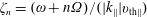 $\unicode[STIX]{x1D701}_{n}=(\unicode[STIX]{x1D714}+n\unicode[STIX]{x1D6FA})/(|k_{\Vert }|v_{\text{th}\Vert })$
. No new discussion on how to treat this singularity is required. The singular point
$\unicode[STIX]{x1D701}_{n}=(\unicode[STIX]{x1D714}+n\unicode[STIX]{x1D6FA})/(|k_{\Vert }|v_{\text{th}\Vert })$
. No new discussion on how to treat this singularity is required. The singular point
 $x_{0}$
in the complex plane is only moved to some other location, and all the previous discussion about the Landau integral fully applies. We could potentially integrate over all the ion-cyclotron resonances and obtain expressions for the heat flux or the fourth-order moments (with the same techniques as plasma physics books do, even though they usually stop at the first-order velocity moment, since it is enough to obtain the kinetic dispersion relation). Even though complicated in detail, these would be just standard kinetic calculations. The difference between the advanced fluid and kinetic descriptions is that we need to find a closure after all of these kinetic calculations, i.e. we need to find a way to express the last considered moment through lower-order moments, such that the closure is valid for all the
$x_{0}$
in the complex plane is only moved to some other location, and all the previous discussion about the Landau integral fully applies. We could potentially integrate over all the ion-cyclotron resonances and obtain expressions for the heat flux or the fourth-order moments (with the same techniques as plasma physics books do, even though they usually stop at the first-order velocity moment, since it is enough to obtain the kinetic dispersion relation). Even though complicated in detail, these would be just standard kinetic calculations. The difference between the advanced fluid and kinetic descriptions is that we need to find a closure after all of these kinetic calculations, i.e. we need to find a way to express the last considered moment through lower-order moments, such that the closure is valid for all the
 $\unicode[STIX]{x1D701}$
values, for example, by using the Padé approximation for
$\unicode[STIX]{x1D701}$
values, for example, by using the Padé approximation for
 $R(\unicode[STIX]{x1D701})$
. Such a closure remains elusive for the ion-cyclotron resonances.
$R(\unicode[STIX]{x1D701})$
. Such a closure remains elusive for the ion-cyclotron resonances.
(iii) Advanced fluid models are not restricted to work with
 $f^{(1)}$
in the gyrotropic limit (4.14). In the Landau fluid models of Passot & Sulem (Reference Passot and Sulem2007), no assumption about the size of the gyroradius is made, and only the low-frequency condition is used and, therefore, the
$f^{(1)}$
in the gyrotropic limit (4.14). In the Landau fluid models of Passot & Sulem (Reference Passot and Sulem2007), no assumption about the size of the gyroradius is made, and only the low-frequency condition is used and, therefore, the
 $f^{(1)}$
of these fluid models contain Bessel functions
$f^{(1)}$
of these fluid models contain Bessel functions
 $\text{J}_{n}(\unicode[STIX]{x1D706}_{r})$
. The integrals over
$\text{J}_{n}(\unicode[STIX]{x1D706}_{r})$
. The integrals over
 $\text{d}v_{\bot }$
are slightly more difficult, and for example if a term proportional to
$\text{d}v_{\bot }$
are slightly more difficult, and for example if a term proportional to
 $\text{J}_{0}(\unicode[STIX]{x1D706})\text{J}_{0}(\unicode[STIX]{x1D706})f_{0}$
is encountered, the integration over
$\text{J}_{0}(\unicode[STIX]{x1D706})\text{J}_{0}(\unicode[STIX]{x1D706})f_{0}$
is encountered, the integration over
 $\text{d}v_{\bot }$
(
$\text{d}v_{\bot }$
(
 $\text{d}^{3}v=v_{\bot }\,\text{d}v_{\bot }\,\text{d}v_{\Vert }\,\text{d}\unicode[STIX]{x1D719}$
) is calculated as
$\text{d}^{3}v=v_{\bot }\,\text{d}v_{\bot }\,\text{d}v_{\Vert }\,\text{d}\unicode[STIX]{x1D719}$
) is calculated as
 $$\begin{eqnarray}\int _{0}^{\infty }x\text{J}_{n}^{2}(ax)e^{-x^{2}}\,\text{d}x={\textstyle \frac{1}{2}}e^{-a^{2}/2}\text{I}_{n}(a^{2}/2),\end{eqnarray}$$
implying
 $$\begin{eqnarray}\displaystyle \int _{0}^{\infty }\text{J}_{0}^{2}\left(\frac{k_{\bot }}{\unicode[STIX]{x1D6FA}}v_{\bot }\right)e^{-\unicode[STIX]{x1D6FC}_{\bot }v_{\bot }^{2}}v_{\bot }\,\text{d}v_{\bot } & = & \displaystyle \left[x=\sqrt{\unicode[STIX]{x1D6FC}_{\bot }}v_{\bot }\right]=\frac{1}{\unicode[STIX]{x1D6FC}_{\bot }}\int _{0}^{\infty }\text{J}_{0}^{2}\left(\frac{k_{\bot }}{\unicode[STIX]{x1D6FA}\sqrt{\unicode[STIX]{x1D6FC}_{\bot }}}x\right)e^{-x^{2}}x\,\text{d}x\nonumber\\ \displaystyle & = & \displaystyle \frac{1}{2\unicode[STIX]{x1D6FC}_{\bot }}e^{-b}\text{I}_{0}(b),\end{eqnarray}$$
where the new parameter
 $b$
(which should not be confused with the magnetic field unit vector
$b$
(which should not be confused with the magnetic field unit vector
 $\hat{\boldsymbol{b}}$
) is
$\hat{\boldsymbol{b}}$
) is
 $$\begin{eqnarray}b=\frac{k_{\bot }^{2}}{2\unicode[STIX]{x1D6FA}^{2}\unicode[STIX]{x1D6FC}_{\bot }}=\frac{k_{\bot }^{2}v_{\text{th}\bot }^{2}}{2\unicode[STIX]{x1D6FA}^{2}}=\frac{k_{\bot }^{2}T_{\bot }^{(0)}}{m\unicode[STIX]{x1D6FA}^{2}}=\frac{1}{2}k_{\bot }^{2}r_{L}^{2}.\end{eqnarray}$$
Calculations like this lead to the functions
 $\unicode[STIX]{x1D6E4}_{0}(b)=e^{-b}\text{I}_{0}(b)$
and
$\unicode[STIX]{x1D6E4}_{0}(b)=e^{-b}\text{I}_{0}(b)$
and
 $\unicode[STIX]{x1D6E4}_{1}(b)=e^{-b}\text{I}_{1}(b)$
. We note that the limit
$\unicode[STIX]{x1D6E4}_{1}(b)=e^{-b}\text{I}_{1}(b)$
. We note that the limit
 $b\rightarrow 0$
yields
$b\rightarrow 0$
yields
 $\unicode[STIX]{x1D6E4}_{0}(b)\rightarrow 1$
and
$\unicode[STIX]{x1D6E4}_{0}(b)\rightarrow 1$
and
 $\unicode[STIX]{x1D6E4}_{1}(b)\rightarrow 0$
.
$\unicode[STIX]{x1D6E4}_{1}(b)\rightarrow 0$
.
4.2 Coulomb force and mirror force (Landau damping and transit-time damping)
The gyrotropic limit (4.14) has a very meaningful physical interpretation. To clearly understand what kind of forces are present in such a system, one needs to consider that a particle quickly gyrates around its slower moving centre, called the ‘guiding centre’, and express the full velocity of a particle
 $\boldsymbol{v}$
as being composed of the quick gyration
$\boldsymbol{v}$
as being composed of the quick gyration
 $\boldsymbol{v}_{\text{gyro}}$
, and a motion of the guiding centre, that is further decomposed to its free motion parallel to the magnetic field line
$\boldsymbol{v}_{\text{gyro}}$
, and a motion of the guiding centre, that is further decomposed to its free motion parallel to the magnetic field line
 $v_{\Vert }\hat{\boldsymbol{b}}$
, and all the possible drifts of the guiding centre: the
$v_{\Vert }\hat{\boldsymbol{b}}$
, and all the possible drifts of the guiding centre: the
 $ExB$
drift
$ExB$
drift
 $\boldsymbol{u}_{E}$
, the grad-
$\boldsymbol{u}_{E}$
, the grad-
 $B$
drift, the curvature drift, the polarization drift etc. The plasma physics books by Fitzpatrick and Gurnett & Bhattacharjee (Reference Gurnett and Bhattacharjee2005) have detailed introductions about single-particle motions in the presence of a Lorentz force, where the drifts of the guiding centre are calculated. Then one should follow the gyrofluid approach, and by performing integrals over
$B$
drift, the curvature drift, the polarization drift etc. The plasma physics books by Fitzpatrick and Gurnett & Bhattacharjee (Reference Gurnett and Bhattacharjee2005) have detailed introductions about single-particle motions in the presence of a Lorentz force, where the drifts of the guiding centre are calculated. Then one should follow the gyrofluid approach, and by performing integrals over
 $\text{d}\unicode[STIX]{x1D719}$
(gyro-averaging) and by expanding for example with respect to Larmor radius, one should get the ‘guiding-centre limit’ of the Vlasov equation and the expression for
$\text{d}\unicode[STIX]{x1D719}$
(gyro-averaging) and by expanding for example with respect to Larmor radius, one should get the ‘guiding-centre limit’ of the Vlasov equation and the expression for
 $f^{(1)}$
. One should follow Kulsrud (Reference Kulsrud, Galeev and Sudan1983), Snyder et al. (Reference Snyder, Hammett and Dorland1997) etc. A very useful paper is also that of Ferrière & André (Reference Ferrière and André2002), that explores the discrepancy between the usual CGL and the long-wavelength low-frequency kinetic theory in great detail and that we follow here.
$f^{(1)}$
. One should follow Kulsrud (Reference Kulsrud, Galeev and Sudan1983), Snyder et al. (Reference Snyder, Hammett and Dorland1997) etc. A very useful paper is also that of Ferrière & André (Reference Ferrière and André2002), that explores the discrepancy between the usual CGL and the long-wavelength low-frequency kinetic theory in great detail and that we follow here.
Without going through the lengthy derivation, it can be shown that at the leading order (for low frequencies
 $\unicode[STIX]{x1D714}/\unicode[STIX]{x1D6FA}$
and long wavelengths
$\unicode[STIX]{x1D714}/\unicode[STIX]{x1D6FA}$
and long wavelengths
 $kr_{L}$
), it is sufficient to consider the motion of the guiding centre with velocity
$kr_{L}$
), it is sufficient to consider the motion of the guiding centre with velocity
 $$\begin{eqnarray}\boldsymbol{v}=v_{\Vert }\hat{\boldsymbol{b}}+\boldsymbol{u}_{E};\quad \boldsymbol{u}_{E}=c\frac{\boldsymbol{E}\times \boldsymbol{B}}{|\boldsymbol{B}|^{2}},\end{eqnarray}$$
where the perpendicular equation of motion satisfies the conservation of the magnetic moment
 $$\begin{eqnarray}\unicode[STIX]{x1D707}=\frac{mv_{\bot }^{2}}{2|\boldsymbol{B}|}=\text{const}.;\quad \Rightarrow \quad \frac{\text{d}}{\text{d}t}\left(\frac{v_{\bot }^{2}}{|\boldsymbol{B}|}\right)=0;\quad \Rightarrow \quad \frac{\text{d}v_{\bot }}{\text{d}t}=\frac{v_{\bot }}{2|\boldsymbol{B}|}\frac{\text{d}|\boldsymbol{B}|}{\text{d}t},\end{eqnarray}$$
and the parallel equation of motion satisfies
 $$\begin{eqnarray}m\frac{\text{d}v_{\Vert }}{\text{d}t}=qE_{\Vert }-\unicode[STIX]{x1D707}\hat{\boldsymbol{b}}\boldsymbol{\cdot }\unicode[STIX]{x1D735}|\boldsymbol{B}|-m\hat{\boldsymbol{b}}\boldsymbol{\cdot }\frac{\text{d}\boldsymbol{u}_{E}}{\text{d}t},\end{eqnarray}$$
where
 $E_{\Vert }=\hat{\boldsymbol{b}}\boldsymbol{\cdot }\boldsymbol{E}$
and
$E_{\Vert }=\hat{\boldsymbol{b}}\boldsymbol{\cdot }\boldsymbol{E}$
and
 $\text{d}/\text{d}t=\unicode[STIX]{x2202}/\unicode[STIX]{x2202}t+\boldsymbol{v}\boldsymbol{\cdot }\unicode[STIX]{x1D735}=\unicode[STIX]{x2202}/\unicode[STIX]{x2202}t+(v_{\Vert }\hat{\boldsymbol{b}}+\boldsymbol{u}_{E})\boldsymbol{\cdot }\unicode[STIX]{x1D735}$
. The first term on the right-hand side of the above equation is the Coulomb force, responsible for acceleration of particles along the magnetic field lines. The second term is the magnetic mirror force, responsible for trapping of particles in the magnetic bottle. The third term is a non-inertial force associated with the time dependence of the
$\text{d}/\text{d}t=\unicode[STIX]{x2202}/\unicode[STIX]{x2202}t+\boldsymbol{v}\boldsymbol{\cdot }\unicode[STIX]{x1D735}=\unicode[STIX]{x2202}/\unicode[STIX]{x2202}t+(v_{\Vert }\hat{\boldsymbol{b}}+\boldsymbol{u}_{E})\boldsymbol{\cdot }\unicode[STIX]{x1D735}$
. The first term on the right-hand side of the above equation is the Coulomb force, responsible for acceleration of particles along the magnetic field lines. The second term is the magnetic mirror force, responsible for trapping of particles in the magnetic bottle. The third term is a non-inertial force associated with the time dependence of the
 $ExB$
drift of the gyrocentre. The similarity of the Coulomb force and the magnetic mirror force can be emphasized by using the scalar potential
$ExB$
drift of the gyrocentre. The similarity of the Coulomb force and the magnetic mirror force can be emphasized by using the scalar potential
 $\unicode[STIX]{x1D6F7}$
and rewriting
$\unicode[STIX]{x1D6F7}$
and rewriting
 $E_{\Vert }=-\unicode[STIX]{x1D735}\unicode[STIX]{x1D6F7}$
, which yields
$E_{\Vert }=-\unicode[STIX]{x1D735}\unicode[STIX]{x1D6F7}$
, which yields
 $$\begin{eqnarray}m\frac{\text{d}v_{\Vert }}{\text{d}t}=\underbrace{-q\hat{\boldsymbol{b}}\boldsymbol{\cdot }\unicode[STIX]{x1D735}\unicode[STIX]{x1D6F7}}_{\text{Coulomb}}\underbrace{-\unicode[STIX]{x1D707}\hat{\boldsymbol{b}}\boldsymbol{\cdot }\unicode[STIX]{x1D735}|\boldsymbol{B}|}_{\text{mirror}}-m\hat{\boldsymbol{b}}\boldsymbol{\cdot }\frac{\text{d}\boldsymbol{u}_{E}}{\text{d}t}.\end{eqnarray}$$
The similarity is immediately apparent, one just needs to replace the charge of the particle with its magnetic moment
 $q\rightarrow \unicode[STIX]{x1D707}$
and replace
$q\rightarrow \unicode[STIX]{x1D707}$
and replace
 $\unicode[STIX]{x1D6F7}\rightarrow |\boldsymbol{B}|$
. Therefore, in a similar way to a charged particle reacting to electric field, a gyrating particle has a magnetic moment that reacts with the gradient of the strength (absolute value) of the magnetic field. The damping effects associated with the Coulomb force are called Landau damping. The damping effects associated with the mirror force are called transit-time damping or Barnes damping (Barnes Reference Barnes1966). Therefore, it is often stated that the transit-time damping is a ‘magnetic analogue’ of Landau damping. Often, the two effects are not separated since both represent the
$\unicode[STIX]{x1D6F7}\rightarrow |\boldsymbol{B}|$
. Therefore, in a similar way to a charged particle reacting to electric field, a gyrating particle has a magnetic moment that reacts with the gradient of the strength (absolute value) of the magnetic field. The damping effects associated with the Coulomb force are called Landau damping. The damping effects associated with the mirror force are called transit-time damping or Barnes damping (Barnes Reference Barnes1966). Therefore, it is often stated that the transit-time damping is a ‘magnetic analogue’ of Landau damping. Often, the two effects are not separated since both represent the
 $n=0$
particle resonance and one talks only about Landau damping. Nevertheless, it is emphasized that Landau fluid models in a 3-D geometry contain both damping mechanisms, and these models contain both the Coulomb force and the mirror force.Footnote
11
$n=0$
particle resonance and one talks only about Landau damping. Nevertheless, it is emphasized that Landau fluid models in a 3-D geometry contain both damping mechanisms, and these models contain both the Coulomb force and the mirror force.Footnote
11
The equations of motion (4.24), (4.25) should be used in the gyro-averaged Vlasov equation
 $$\begin{eqnarray}\frac{\unicode[STIX]{x2202}f}{\unicode[STIX]{x2202}t}+(v_{\Vert }\hat{\boldsymbol{b}}+\boldsymbol{u}_{E})\boldsymbol{\cdot }\unicode[STIX]{x1D735}f+\left[\frac{\text{d}v_{\bot }}{\text{d}t}\frac{\unicode[STIX]{x2202}}{\unicode[STIX]{x2202}v_{\bot }}+\frac{\text{d}v_{\Vert }}{\text{d}t}\frac{\unicode[STIX]{x2202}}{\unicode[STIX]{x2202}v_{\Vert }}\right]f=0,\end{eqnarray}$$
and the equation should be expanded
 $f=f_{0}+f^{(1)}$
. We are interested only in linear solutions, and we can simplify. To avoid discussing compatibility conditions for
$f=f_{0}+f^{(1)}$
. We are interested only in linear solutions, and we can simplify. To avoid discussing compatibility conditions for
 $f_{0}$
(see Kulsrud Reference Kulsrud, Galeev and Sudan1983), we can just simply claim that
$f_{0}$
(see Kulsrud Reference Kulsrud, Galeev and Sudan1983), we can just simply claim that
 $f_{0}$
does not have any time or spatial dependence. By further noticing that linearization of
$f_{0}$
does not have any time or spatial dependence. By further noticing that linearization of
 $\boldsymbol{u}_{E}\overset{\text{lin}}{=}\boldsymbol{u}_{E}^{(0)}+\boldsymbol{u}_{E}^{(1)}$
yields
$\boldsymbol{u}_{E}\overset{\text{lin}}{=}\boldsymbol{u}_{E}^{(0)}+\boldsymbol{u}_{E}^{(1)}$
yields
 $\boldsymbol{u}_{E}^{(0)}=c\boldsymbol{E}_{0}\times \boldsymbol{B}_{0}/B_{0}^{2}=0$
since
$\boldsymbol{u}_{E}^{(0)}=c\boldsymbol{E}_{0}\times \boldsymbol{B}_{0}/B_{0}^{2}=0$
since
 $E_{0}=0$
, we can immediately write that at the linear level
$E_{0}=0$
, we can immediately write that at the linear level
 $$\begin{eqnarray}\frac{\unicode[STIX]{x2202}f^{(1)}}{\unicode[STIX]{x2202}t}+v_{\Vert }\unicode[STIX]{x2202}_{z}f^{(1)}=-\left[\frac{\text{d}v_{\bot }}{\text{d}t}\frac{\unicode[STIX]{x2202}}{\unicode[STIX]{x2202}v_{\bot }}+\frac{\text{d}v_{\Vert }}{\text{d}t}\frac{\unicode[STIX]{x2202}}{\unicode[STIX]{x2202}v_{\Vert }}\right]f_{0}.\end{eqnarray}$$
Noticing that the
 $ExB$
drift
$ExB$
drift
 $\boldsymbol{u}_{E}$
is always perpendicular to the direction of
$\boldsymbol{u}_{E}$
is always perpendicular to the direction of
 $\boldsymbol{B}$
(and also
$\boldsymbol{B}$
(and also
 $\boldsymbol{E}$
) implies
$\boldsymbol{E}$
) implies
 $\hat{\boldsymbol{b}}\boldsymbol{\cdot }\boldsymbol{u}_{E}=0$
, and the last term in the
$\hat{\boldsymbol{b}}\boldsymbol{\cdot }\boldsymbol{u}_{E}=0$
, and the last term in the
 $\text{d}v_{\Vert }/\text{d}t$
equation (4.25) rewrites as
$\text{d}v_{\Vert }/\text{d}t$
equation (4.25) rewrites as
 $$\begin{eqnarray}-\hat{\boldsymbol{b}}\boldsymbol{\cdot }\frac{\text{d}\boldsymbol{u}_{E}}{\text{d}t}=-\frac{\text{d}}{\text{d}t}(\underbrace{\hat{\boldsymbol{b}}\boldsymbol{\cdot }\boldsymbol{u}_{E}}_{=0})+\boldsymbol{u}_{E}\boldsymbol{\cdot }\frac{\text{d}\hat{\boldsymbol{b}}}{\text{d}t},\end{eqnarray}$$
which at the linear level disappears, since
 $$\begin{eqnarray}\boldsymbol{u}_{E}\boldsymbol{\cdot }\frac{\text{d}\hat{\boldsymbol{b}}}{\text{d}t}\overset{\text{lin}}{=}\underbrace{\boldsymbol{u}_{E}^{(0)}}_{=0}\boldsymbol{\cdot }\frac{\text{d}\hat{\boldsymbol{b}}^{(1)}}{\text{d}t}+\boldsymbol{u}_{E}^{(1)}\boldsymbol{\cdot }\underbrace{\frac{\text{d}\hat{\boldsymbol{b}}^{(0)}}{\text{d}t}}_{=0}=0.\end{eqnarray}$$
The magnetic mirror force contains
 $\unicode[STIX]{x2202}_{z}|\boldsymbol{B}|=\unicode[STIX]{x2202}_{z}\sqrt{B_{x}^{2}+B_{y}^{2}+B_{z}^{2}}=\hat{\boldsymbol{b}}\boldsymbol{\cdot }\unicode[STIX]{x2202}_{z}\boldsymbol{B}$
, where linearization yields
$\unicode[STIX]{x2202}_{z}|\boldsymbol{B}|=\unicode[STIX]{x2202}_{z}\sqrt{B_{x}^{2}+B_{y}^{2}+B_{z}^{2}}=\hat{\boldsymbol{b}}\boldsymbol{\cdot }\unicode[STIX]{x2202}_{z}\boldsymbol{B}$
, where linearization yields
 $\unicode[STIX]{x2202}_{z}|\boldsymbol{B}|\overset{\text{lin}}{=}\unicode[STIX]{x2202}_{z}B_{z}$
. Similarly, the
$\unicode[STIX]{x2202}_{z}|\boldsymbol{B}|\overset{\text{lin}}{=}\unicode[STIX]{x2202}_{z}B_{z}$
. Similarly, the
 $\text{d}v_{\bot }/\text{d}t$
equation (4.24) contains
$\text{d}v_{\bot }/\text{d}t$
equation (4.24) contains
 $\text{d}|\boldsymbol{B}|/\text{d}t=\hat{\boldsymbol{b}}\boldsymbol{\cdot }\text{d}\boldsymbol{B}/\text{d}t$
that linearizes as
$\text{d}|\boldsymbol{B}|/\text{d}t=\hat{\boldsymbol{b}}\boldsymbol{\cdot }\text{d}\boldsymbol{B}/\text{d}t$
that linearizes as
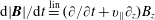 $\text{d}|\boldsymbol{B}|/\text{d}t\overset{\text{lin}}{=}(\unicode[STIX]{x2202}/\unicode[STIX]{x2202}t+v_{\Vert }\unicode[STIX]{x2202}_{z})B_{z}$
. The linearized equations of motion therefore read
$\text{d}|\boldsymbol{B}|/\text{d}t\overset{\text{lin}}{=}(\unicode[STIX]{x2202}/\unicode[STIX]{x2202}t+v_{\Vert }\unicode[STIX]{x2202}_{z})B_{z}$
. The linearized equations of motion therefore read
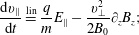 $$\begin{eqnarray}\displaystyle & \displaystyle \frac{\text{d}v_{\Vert }}{\text{d}t}\overset{\text{lin}}{=}\frac{q}{m}E_{\Vert }-\frac{v_{\bot }^{2}}{2B_{0}}\unicode[STIX]{x2202}_{z}B_{z}; & \displaystyle\end{eqnarray}$$
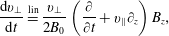 $$\begin{eqnarray}\displaystyle & \displaystyle \frac{\text{d}v_{\bot }}{\text{d}t}\overset{\text{lin}}{=}\frac{v_{\bot }}{2B_{0}}\left(\frac{\unicode[STIX]{x2202}}{\unicode[STIX]{x2202}t}+v_{\Vert }\unicode[STIX]{x2202}_{z}\right)B_{z}, & \displaystyle\end{eqnarray}$$
yielding the final expression for
 $f^{(1)}$
in real space
$f^{(1)}$
in real space
 $$\begin{eqnarray}\left(\frac{\unicode[STIX]{x2202}}{\unicode[STIX]{x2202}t}+v_{\Vert }\unicode[STIX]{x2202}_{z}\right)f^{(1)}=-\frac{v_{\bot }}{2B_{0}}\left(\frac{\unicode[STIX]{x2202}}{\unicode[STIX]{x2202}t}+v_{\Vert }\unicode[STIX]{x2202}_{z}\right)B_{z}\frac{\unicode[STIX]{x2202}f_{0}}{\unicode[STIX]{x2202}v_{\bot }}-\left(\frac{q}{m}E_{\Vert }-\frac{v_{\bot }^{2}}{2B_{0}}\unicode[STIX]{x2202}_{z}B_{z}\right)\frac{\unicode[STIX]{x2202}f_{0}}{\unicode[STIX]{x2202}v_{\Vert }},\end{eqnarray}$$
which when Fourier transformed recovers the
 $f^{(1)}$
in the gyrotropic limit (4.14). Instead of fully linearized equations with
$f^{(1)}$
in the gyrotropic limit (4.14). Instead of fully linearized equations with
 $B_{z}$
, one can also work with
$B_{z}$
, one can also work with
 $|\boldsymbol{B}|$
, i.e. one can write the leading-order equations of motion as
$|\boldsymbol{B}|$
, i.e. one can write the leading-order equations of motion as
 $$\begin{eqnarray}\displaystyle & \displaystyle \frac{\text{d}v_{\Vert }}{\text{d}t}=\frac{q}{m}E_{\Vert }-\frac{v_{\bot }^{2}}{2B_{0}}\unicode[STIX]{x2202}_{z}|\boldsymbol{B}|; & \displaystyle\end{eqnarray}$$
 $$\begin{eqnarray}\displaystyle & \displaystyle \frac{\text{d}v_{\bot }}{\text{d}t}=\frac{v_{\bot }}{2B_{0}}\left(\frac{\unicode[STIX]{x2202}}{\unicode[STIX]{x2202}t}+v_{\Vert }\unicode[STIX]{x2202}_{z}\right)|\boldsymbol{B}|, & \displaystyle\end{eqnarray}$$
which yields analogous equations (4.33), (4.14) where
 $B_{z}$
is just replaced by
$B_{z}$
is just replaced by
 $|\boldsymbol{B}|$
.
$|\boldsymbol{B}|$
.
4.3 Kinetic moments for bi-Maxwellian
$f_{0}$

Since in the Vlasov expansion the gyrotropic
 $f_{0}$
was assumed to depended only on
$f_{0}$
was assumed to depended only on
 $\boldsymbol{v}$
, i.e.
$\boldsymbol{v}$
, i.e.
 $f_{0}(v_{\bot }^{2},v_{\Vert }^{2})$
and be
$f_{0}(v_{\bot }^{2},v_{\Vert }^{2})$
and be
 $\boldsymbol{x},t$
independent, the fluid velocity
$\boldsymbol{x},t$
independent, the fluid velocity
 $\boldsymbol{u}$
is removed from the distribution function and the ‘pure’ bi-Maxwellian is
$\boldsymbol{u}$
is removed from the distribution function and the ‘pure’ bi-Maxwellian is
 $$\begin{eqnarray}\displaystyle f_{0}=n_{0}\sqrt{\frac{\unicode[STIX]{x1D6FC}_{\Vert }}{\unicode[STIX]{x03C0}}}\frac{\unicode[STIX]{x1D6FC}_{\bot }}{\unicode[STIX]{x03C0}}e^{-\unicode[STIX]{x1D6FC}_{\Vert }v_{\Vert }^{2}-\unicode[STIX]{x1D6FC}_{\bot }v_{\bot }^{2}}, & & \displaystyle\end{eqnarray}$$
where
 $$\begin{eqnarray}\unicode[STIX]{x1D6FC}_{\Vert }=\frac{m}{2T_{\Vert }^{(0)}};\quad \unicode[STIX]{x1D6FC}_{\bot }=\frac{m}{2T_{\bot }^{(0)}},\end{eqnarray}$$
or in the language of thermal speeds,
 $$\begin{eqnarray}v_{\text{th}\Vert }^{2}=\frac{2T_{\Vert }^{(0)}}{m}=\unicode[STIX]{x1D6FC}_{\Vert }^{-1};\quad v_{\text{th}\bot }^{2}=\frac{2T_{\bot }^{(0)}}{m}=\unicode[STIX]{x1D6FC}_{\bot }^{-1}.\end{eqnarray}$$
We prefer the
 $\unicode[STIX]{x1D6FC}$
notation instead of the thermal speed
$\unicode[STIX]{x1D6FC}$
notation instead of the thermal speed
 $v_{\text{th}}$
, since in long analytic calculations, there is a lesser chance of an error. We work without the species index
$v_{\text{th}}$
, since in long analytic calculations, there is a lesser chance of an error. We work without the species index
 $r$
except for charge
$r$
except for charge
 $q_{r}$
and mass
$q_{r}$
and mass
 $m_{r}$
. It is straightforward to calculate that
$m_{r}$
. It is straightforward to calculate that
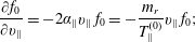 $$\begin{eqnarray}\displaystyle & \displaystyle \frac{\unicode[STIX]{x2202}f_{0}}{\unicode[STIX]{x2202}v_{\Vert }}=-2\unicode[STIX]{x1D6FC}_{\Vert }v_{\Vert }\,f_{0}=-\frac{m_{r}}{T_{\Vert }^{(0)}}v_{\Vert }\,f_{0}; & \displaystyle\end{eqnarray}$$
 $$\begin{eqnarray}\displaystyle & \displaystyle \frac{\unicode[STIX]{x2202}f_{0}}{\unicode[STIX]{x2202}v_{\bot }}=-2\unicode[STIX]{x1D6FC}_{\bot }v_{\bot }\,f_{0}=-\frac{m_{r}}{T_{\bot }^{(0)}}v_{\bot }\,f_{0}. & \displaystyle\end{eqnarray}$$
Instead of
 $E_{z}$
, we will work with the scalar potential
$E_{z}$
, we will work with the scalar potential
 $\unicode[STIX]{x1D6F7}$
as before
$\unicode[STIX]{x1D6F7}$
as before
 $$\begin{eqnarray}E_{z}=-\unicode[STIX]{x1D735}_{\Vert }\unicode[STIX]{x1D6F7};\quad \Rightarrow \quad iE_{z}=k_{\Vert }\unicode[STIX]{x1D6F7}.\end{eqnarray}$$
The
 $f^{(1)}$
that we want to integrate reads
$f^{(1)}$
that we want to integrate reads
 $$\begin{eqnarray}f^{(1)}=\frac{B_{z}}{B_{0}}\unicode[STIX]{x1D6FC}_{\bot }\left[v_{\bot }^{2}f_{0}+\frac{\unicode[STIX]{x1D6FC}_{\Vert }}{\unicode[STIX]{x1D6FC}_{\bot }}\frac{k_{\Vert }v_{\Vert }v_{\bot }^{2}}{(\unicode[STIX]{x1D714}-k_{\Vert }v_{\Vert })}f_{0}\right]+\unicode[STIX]{x1D6F7}\frac{q_{r}}{m_{r}}2\unicode[STIX]{x1D6FC}_{\Vert }\frac{k_{\Vert }v_{\Vert }}{(\unicode[STIX]{x1D714}-k_{\Vert }v_{\Vert })}f_{0},\end{eqnarray}$$
or alternatively expressed with temperatures
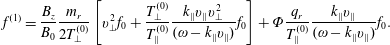 $$\begin{eqnarray}f^{(1)}=\frac{B_{z}}{B_{0}}\frac{m_{r}}{2T_{\bot }^{(0)}}\left[v_{\bot }^{2}f_{0}+\frac{T_{\bot }^{(0)}}{T_{\Vert }^{(0)}}\frac{k_{\Vert }v_{\Vert }v_{\bot }^{2}}{(\unicode[STIX]{x1D714}-k_{\Vert }v_{\Vert })}f_{0}\right]+\unicode[STIX]{x1D6F7}\frac{q_{r}}{T_{\Vert }^{(0)}}\frac{k_{\Vert }v_{\Vert }}{(\unicode[STIX]{x1D714}-k_{\Vert }v_{\Vert })}f_{0}.\end{eqnarray}$$
Now we want to calculate the linear ‘kinetic’ moments over this distribution function. The kinetic moments are
 $$\begin{eqnarray}n^{(1)}=\int f^{(1)}\text{d}^{3}v;\quad u_{\Vert }^{(1)}=\frac{1}{n_{0}}\int v_{\Vert }f^{(1)}\,\text{d}^{3}v;\end{eqnarray}$$
 $$\begin{eqnarray}p_{\Vert }^{(1)}=m_{r}\int v_{\Vert }^{2}f^{(1)}\,\text{d}^{3}v;\quad p_{\bot }^{(1)}=\frac{m_{r}}{2}\int v_{\bot }^{2}f^{(1)}\,\text{d}^{3}v;\end{eqnarray}$$
 $$\begin{eqnarray}q_{\Vert }^{(1)}=m_{r}\int v_{\Vert }^{3}f^{(1)}\,\text{d}^{3}v-3p_{\Vert }^{(0)}u_{\Vert }^{(1)};\quad q_{\bot }^{(1)}=\frac{m_{r}}{2}\int v_{\Vert }v_{\bot }^{2}f^{(1)}\,\text{d}^{3}v-p_{\bot }^{(0)}u_{\Vert }^{(1)};\end{eqnarray}$$
 $$\begin{eqnarray}r_{\Vert \Vert }^{(1)}=m_{r}\int v_{\Vert }^{4}f^{(1)}\,\text{d}^{3}v;\quad r_{\Vert \bot }^{(1)}=\frac{m_{r}}{2}\int v_{\Vert }^{2}v_{\bot }^{2}f^{(1)}\,\text{d}^{3}v;\quad r_{\bot \bot }^{(1)}=\frac{m_{r}}{4}\int v_{\bot }^{4}f^{(1)}\,\text{d}^{3}v.\end{eqnarray}$$
We have so far avoided integration in the cylindrical coordinate system, and all the previous integrals were done in the Cartesian coordinate system. In the cylindrical system,
 $\text{d}^{3}v=v_{\bot }\,\text{d}v_{\bot }\,\text{d}v_{\Vert }\,\text{d}\unicode[STIX]{x1D719}$
and the integral with respect to
$\text{d}^{3}v=v_{\bot }\,\text{d}v_{\bot }\,\text{d}v_{\Vert }\,\text{d}\unicode[STIX]{x1D719}$
and the integral with respect to
 $v_{\bot }$
is from 0 to
$v_{\bot }$
is from 0 to
 $\infty$
. The Gaussian integrals are
$\infty$
. The Gaussian integrals are
 $$\begin{eqnarray}\displaystyle \displaystyle \int _{0}^{\infty }e^{-ax^{2}}\,\text{d}x=\frac{1}{2}\sqrt{\frac{\unicode[STIX]{x03C0}}{a}};\quad \int _{0}^{\infty }xe^{-ax^{2}}\,\text{d}x=\frac{1}{2a}; & & \displaystyle \nonumber\\ \displaystyle \displaystyle \int _{0}^{\infty }x^{2}e^{-ax^{2}}\,\text{d}x=\frac{1}{4a}\sqrt{\frac{\unicode[STIX]{x03C0}}{a}};\quad \int _{0}^{\infty }x^{3}e^{-ax^{2}}\,\text{d}x=\frac{1}{2a^{2}}; & & \displaystyle \nonumber\\ \displaystyle \displaystyle \int _{0}^{\infty }x^{4}e^{-ax^{2}}\,\text{d}x=\frac{3}{8a^{2}}\sqrt{\frac{\unicode[STIX]{x03C0}}{a}};\quad \int _{0}^{\infty }x^{5}e^{-ax^{2}}\,\text{d}x=\frac{1}{a^{3}}; & & \displaystyle \nonumber\\ \displaystyle \displaystyle \int _{0}^{\infty }x^{6}e^{-ax^{2}}\,\text{d}x=\frac{15}{16a^{3}}\sqrt{\frac{\unicode[STIX]{x03C0}}{a}};\quad \int _{0}^{\infty }x^{7}e^{-ax^{2}}\,\text{d}x=\frac{3}{a^{4}}. & & \displaystyle \nonumber\end{eqnarray}$$
Therefore, integrating over
 $\text{d}v_{\bot }\,\text{d}\unicode[STIX]{x1D719}$
is straightforward and
$\text{d}v_{\bot }\,\text{d}\unicode[STIX]{x1D719}$
is straightforward and
 $$\begin{eqnarray}\displaystyle \int f_{0}v_{\bot }\,\text{d}v_{\bot }\,\text{d}\unicode[STIX]{x1D719} & = & \displaystyle 2\unicode[STIX]{x03C0}\int _{0}^{\infty }f_{0}v_{\bot }\,\text{d}v_{\bot }\nonumber\\ \displaystyle & = & \displaystyle 2\unicode[STIX]{x03C0}n_{0}\sqrt{\frac{\unicode[STIX]{x1D6FC}_{\Vert }}{\unicode[STIX]{x03C0}}}e^{-\unicode[STIX]{x1D6FC}_{\Vert }v_{\Vert }^{2}}\frac{\unicode[STIX]{x1D6FC}_{\bot }}{\unicode[STIX]{x03C0}}\underbrace{\int _{0}^{\infty }v_{\bot }e^{-\unicode[STIX]{x1D6FC}_{\bot }v_{\bot }^{2}}\,\text{d}v_{\bot }}_{=1/(2\unicode[STIX]{x1D6FC}_{\bot })}=n_{0}\sqrt{\frac{\unicode[STIX]{x1D6FC}_{\Vert }}{\unicode[STIX]{x03C0}}}e^{-\unicode[STIX]{x1D6FC}_{\Vert }v_{\Vert }^{2}},\end{eqnarray}$$
and similarly
 $$\begin{eqnarray}\displaystyle & & \displaystyle \int f_{0}v_{\bot }^{3}\,\text{d}v_{\bot }\,\text{d}\unicode[STIX]{x1D719}=n_{0}\sqrt{\frac{\unicode[STIX]{x1D6FC}_{\Vert }}{\unicode[STIX]{x03C0}}}e^{-\unicode[STIX]{x1D6FC}_{\Vert }v_{\Vert }^{2}}\frac{1}{\unicode[STIX]{x1D6FC}_{\bot }};\quad \int f_{0}v_{\bot }^{5}\,\text{d}v_{\bot }\,\text{d}\unicode[STIX]{x1D719}=n_{0}\sqrt{\frac{\unicode[STIX]{x1D6FC}_{\Vert }}{\unicode[STIX]{x03C0}}}e^{-\unicode[STIX]{x1D6FC}_{\Vert }v_{\Vert }^{2}}\frac{2}{\unicode[STIX]{x1D6FC}_{\bot }^{2}};\nonumber\\ \displaystyle & & \displaystyle \int f_{0}v_{\bot }^{7}\,\text{d}v_{\bot }\,\text{d}\unicode[STIX]{x1D719}=n_{0}\sqrt{\frac{\unicode[STIX]{x1D6FC}_{\Vert }}{\unicode[STIX]{x03C0}}}e^{-\unicode[STIX]{x1D6FC}_{\Vert }v_{\Vert }^{2}}\frac{6}{\unicode[STIX]{x1D6FC}_{\bot }^{3}},\end{eqnarray}$$
and these are all of integrals over
 $\text{d}v_{\bot }$
that are needed right now. The basic integrals (without singularity) calculate as
$\text{d}v_{\bot }$
that are needed right now. The basic integrals (without singularity) calculate as
 $$\begin{eqnarray}\displaystyle & & \displaystyle \int f_{0}\,\text{d}^{3}v=n_{0};\quad \int v_{\Vert }f_{0}\,\text{d}^{3}v=0;\quad \int v_{\Vert }^{2}f_{0}\,\text{d}^{3}v=n_{0}\frac{1}{2\unicode[STIX]{x1D6FC}_{\Vert }};\nonumber\\ \displaystyle & & \displaystyle \int v_{\Vert }^{3}f_{0}\,\text{d}^{3}v=0;\quad \int v_{\Vert }^{4}f_{0}\,\text{d}^{3}v=n_{0}\frac{3}{4\unicode[STIX]{x1D6FC}_{\Vert }^{2}},\end{eqnarray}$$
and each integral yields further 3 cases from (4.49) just by multiplying, so
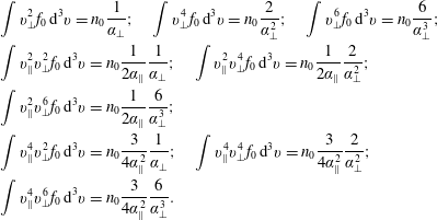 $$\begin{eqnarray}\displaystyle & & \displaystyle \int v_{\bot }^{2}f_{0}\,\text{d}^{3}v=n_{0}\frac{1}{\unicode[STIX]{x1D6FC}_{\bot }};\quad \int v_{\bot }^{4}f_{0}\,\text{d}^{3}v=n_{0}\frac{2}{\unicode[STIX]{x1D6FC}_{\bot }^{2}};\quad \int v_{\bot }^{6}f_{0}\,\text{d}^{3}v=n_{0}\frac{6}{\unicode[STIX]{x1D6FC}_{\bot }^{3}};\nonumber\\ \displaystyle & & \displaystyle \int v_{\Vert }^{2}v_{\bot }^{2}f_{0}\,\text{d}^{3}v=n_{0}\frac{1}{2\unicode[STIX]{x1D6FC}_{\Vert }}\frac{1}{\unicode[STIX]{x1D6FC}_{\bot }};\quad \int v_{\Vert }^{2}v_{\bot }^{4}f_{0}\,\text{d}^{3}v=n_{0}\frac{1}{2\unicode[STIX]{x1D6FC}_{\Vert }}\frac{2}{\unicode[STIX]{x1D6FC}_{\bot }^{2}};\nonumber\\ \displaystyle & & \displaystyle \int v_{\Vert }^{2}v_{\bot }^{6}f_{0}\,\text{d}^{3}v=n_{0}\frac{1}{2\unicode[STIX]{x1D6FC}_{\Vert }}\frac{6}{\unicode[STIX]{x1D6FC}_{\bot }^{3}};\nonumber\\ \displaystyle & & \displaystyle \int v_{\Vert }^{4}v_{\bot }^{2}f_{0}\,\text{d}^{3}v=n_{0}\frac{3}{4\unicode[STIX]{x1D6FC}_{\Vert }^{2}}\frac{1}{\unicode[STIX]{x1D6FC}_{\bot }};\quad \int v_{\Vert }^{4}v_{\bot }^{4}f_{0}\,\text{d}^{3}v=n_{0}\frac{3}{4\unicode[STIX]{x1D6FC}_{\Vert }^{2}}\frac{2}{\unicode[STIX]{x1D6FC}_{\bot }^{2}};\nonumber\\ \displaystyle & & \displaystyle \int v_{\Vert }^{4}v_{\bot }^{6}f_{0}\,\text{d}^{3}v=n_{0}\frac{3}{4\unicode[STIX]{x1D6FC}_{\Vert }^{2}}\frac{6}{\unicode[STIX]{x1D6FC}_{\bot }^{3}}.\end{eqnarray}$$
By using Landau integrals (2.54)–(2.58), the following integrals can be calculated
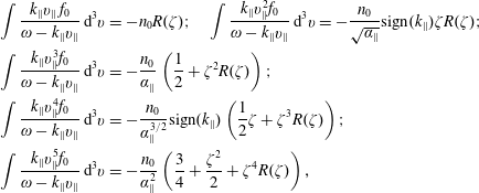 $$\begin{eqnarray}\displaystyle & & \displaystyle \int \frac{k_{\Vert }v_{\Vert }\,f_{0}}{\unicode[STIX]{x1D714}-k_{\Vert }v_{\Vert }}\,\text{d}^{3}v=-n_{0}R(\unicode[STIX]{x1D701});\quad \int \frac{k_{\Vert }v_{\Vert }^{2}f_{0}}{\unicode[STIX]{x1D714}-k_{\Vert }v_{\Vert }}\,\text{d}^{3}v=-\frac{n_{0}}{\sqrt{\unicode[STIX]{x1D6FC}_{\Vert }}}\text{sign}(k_{\Vert })\unicode[STIX]{x1D701}R(\unicode[STIX]{x1D701});\nonumber\\ \displaystyle & & \displaystyle \int \frac{k_{\Vert }v_{\Vert }^{3}f_{0}}{\unicode[STIX]{x1D714}-k_{\Vert }v_{\Vert }}\,\text{d}^{3}v=-\frac{n_{0}}{\unicode[STIX]{x1D6FC}_{\Vert }}\left(\frac{1}{2}+\unicode[STIX]{x1D701}^{2}R(\unicode[STIX]{x1D701})\right);\nonumber\\ \displaystyle & & \displaystyle \int \frac{k_{\Vert }v_{\Vert }^{4}f_{0}}{\unicode[STIX]{x1D714}-k_{\Vert }v_{\Vert }}\,\text{d}^{3}v=-\frac{n_{0}}{\unicode[STIX]{x1D6FC}_{\Vert }^{3/2}}\text{sign}(k_{\Vert })\left(\frac{1}{2}\unicode[STIX]{x1D701}+\unicode[STIX]{x1D701}^{3}R(\unicode[STIX]{x1D701})\right);\nonumber\\ \displaystyle & & \displaystyle \int \frac{k_{\Vert }v_{\Vert }^{5}f_{0}}{\unicode[STIX]{x1D714}-k_{\Vert }v_{\Vert }}\,\text{d}^{3}v=-\frac{n_{0}}{\unicode[STIX]{x1D6FC}_{\Vert }^{2}}\left(\frac{3}{4}+\frac{\unicode[STIX]{x1D701}^{2}}{2}+\unicode[STIX]{x1D701}^{4}R(\unicode[STIX]{x1D701})\right),\end{eqnarray}$$
and each of these integrals yields further 3 cases from (4.49) just by multiplying, so that
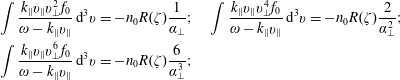 $$\begin{eqnarray}\displaystyle & & \displaystyle \int \frac{k_{\Vert }v_{\Vert }v_{\bot }^{2}f_{0}}{\unicode[STIX]{x1D714}-k_{\Vert }v_{\Vert }}\,\text{d}^{3}v=-n_{0}R(\unicode[STIX]{x1D701})\frac{1}{\unicode[STIX]{x1D6FC}_{\bot }};\quad \int \frac{k_{\Vert }v_{\Vert }v_{\bot }^{4}f_{0}}{\unicode[STIX]{x1D714}-k_{\Vert }v_{\Vert }}\,\text{d}^{3}v=-n_{0}R(\unicode[STIX]{x1D701})\frac{2}{\unicode[STIX]{x1D6FC}_{\bot }^{2}};\nonumber\\ \displaystyle & & \displaystyle \int \frac{k_{\Vert }v_{\Vert }v_{\bot }^{6}f_{0}}{\unicode[STIX]{x1D714}-k_{\Vert }v_{\Vert }}\,\text{d}^{3}v=-n_{0}R(\unicode[STIX]{x1D701})\frac{6}{\unicode[STIX]{x1D6FC}_{\bot }^{3}};\end{eqnarray}$$
 $$\begin{eqnarray}\displaystyle & & \displaystyle \int \frac{k_{\Vert }v_{\Vert }^{2}v_{\bot }^{2}f_{0}}{\unicode[STIX]{x1D714}-k_{\Vert }v_{\Vert }}\,\text{d}^{3}v=-\frac{n_{0}}{\sqrt{\unicode[STIX]{x1D6FC}_{\Vert }}}\text{sign}(k_{\Vert })\unicode[STIX]{x1D701}R(\unicode[STIX]{x1D701})\frac{1}{\unicode[STIX]{x1D6FC}_{\bot }};\nonumber\\ \displaystyle & & \displaystyle \int \frac{k_{\Vert }v_{\Vert }^{2}v_{\bot }^{4}f_{0}}{\unicode[STIX]{x1D714}-k_{\Vert }v_{\Vert }}\,\text{d}^{3}v=-\frac{n_{0}}{\sqrt{\unicode[STIX]{x1D6FC}_{\Vert }}}\text{sign}(k_{\Vert })\unicode[STIX]{x1D701}R(\unicode[STIX]{x1D701})\frac{2}{\unicode[STIX]{x1D6FC}_{\bot }^{2}};\nonumber\\ \displaystyle & & \displaystyle \int \frac{k_{\Vert }v_{\Vert }^{2}v_{\bot }^{6}f_{0}}{\unicode[STIX]{x1D714}-k_{\Vert }v_{\Vert }}\,\text{d}^{3}v=-\frac{n_{0}}{\sqrt{\unicode[STIX]{x1D6FC}_{\Vert }}}\text{sign}(k_{\Vert })\unicode[STIX]{x1D701}R(\unicode[STIX]{x1D701})\frac{6}{\unicode[STIX]{x1D6FC}_{\bot }^{3}};\end{eqnarray}$$
 $$\begin{eqnarray}\displaystyle & & \displaystyle \int \frac{k_{\Vert }v_{\Vert }^{3}v_{\bot }^{2}f_{0}}{\unicode[STIX]{x1D714}-k_{\Vert }v_{\Vert }}\,\text{d}^{3}v=-\frac{n_{0}}{\unicode[STIX]{x1D6FC}_{\Vert }}\left(\frac{1}{2}+\unicode[STIX]{x1D701}^{2}R(\unicode[STIX]{x1D701})\right)\frac{1}{\unicode[STIX]{x1D6FC}_{\bot }};\nonumber\\ \displaystyle & & \displaystyle \int \frac{k_{\Vert }v_{\Vert }^{3}v_{\bot }^{4}f_{0}}{\unicode[STIX]{x1D714}-k_{\Vert }v_{\Vert }}\,\text{d}^{3}v=-\frac{n_{0}}{\unicode[STIX]{x1D6FC}_{\Vert }}\left(\frac{1}{2}+\unicode[STIX]{x1D701}^{2}R(\unicode[STIX]{x1D701})\right)\frac{2}{\unicode[STIX]{x1D6FC}_{\bot }^{2}};\nonumber\\ \displaystyle & & \displaystyle \int \frac{k_{\Vert }v_{\Vert }^{3}v_{\bot }^{6}f_{0}}{\unicode[STIX]{x1D714}-k_{\Vert }v_{\Vert }}\,\text{d}^{3}v=-\frac{n_{0}}{\unicode[STIX]{x1D6FC}_{\Vert }}\left(\frac{1}{2}+\unicode[STIX]{x1D701}^{2}R(\unicode[STIX]{x1D701})\right)\frac{6}{\unicode[STIX]{x1D6FC}_{\bot }^{3}};\end{eqnarray}$$
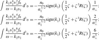 $$\begin{eqnarray}\displaystyle & & \displaystyle \int \frac{k_{\Vert }v_{\Vert }^{4}v_{\bot }^{2}f_{0}}{\unicode[STIX]{x1D714}-k_{\Vert }v_{\Vert }}\,\text{d}^{3}v=-\frac{n_{0}}{\unicode[STIX]{x1D6FC}_{\Vert }^{3/2}}\text{sign}(k_{\Vert })\left(\frac{1}{2}\unicode[STIX]{x1D701}+\unicode[STIX]{x1D701}^{3}R(\unicode[STIX]{x1D701})\right)\frac{1}{\unicode[STIX]{x1D6FC}_{\bot }};\nonumber\\ \displaystyle & & \displaystyle \int \frac{k_{\Vert }v_{\Vert }^{4}v_{\bot }^{4}f_{0}}{\unicode[STIX]{x1D714}-k_{\Vert }v_{\Vert }}\,\text{d}^{3}v=-\frac{n_{0}}{\unicode[STIX]{x1D6FC}_{\Vert }^{3/2}}\text{sign}(k_{\Vert })\left(\frac{1}{2}\unicode[STIX]{x1D701}+\unicode[STIX]{x1D701}^{3}R(\unicode[STIX]{x1D701})\right)\frac{2}{\unicode[STIX]{x1D6FC}_{\bot }^{2}};\nonumber\\ \displaystyle & & \displaystyle \int \frac{k_{\Vert }v_{\Vert }^{4}v_{\bot }^{6}f_{0}}{\unicode[STIX]{x1D714}-k_{\Vert }v_{\Vert }}\,\text{d}^{3}v=-\frac{n_{0}}{\unicode[STIX]{x1D6FC}_{\Vert }^{3/2}}\text{sign}(k_{\Vert })\left(\frac{1}{2}\unicode[STIX]{x1D701}+\unicode[STIX]{x1D701}^{3}R(\unicode[STIX]{x1D701})\right)\frac{6}{\unicode[STIX]{x1D6FC}_{\bot }^{3}};\end{eqnarray}$$
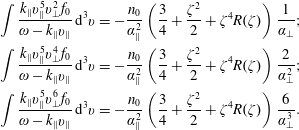 $$\begin{eqnarray}\displaystyle & & \displaystyle \int \frac{k_{\Vert }v_{\Vert }^{5}v_{\bot }^{2}f_{0}}{\unicode[STIX]{x1D714}-k_{\Vert }v_{\Vert }}\,\text{d}^{3}v=-\frac{n_{0}}{\unicode[STIX]{x1D6FC}_{\Vert }^{2}}\left(\frac{3}{4}+\frac{\unicode[STIX]{x1D701}^{2}}{2}+\unicode[STIX]{x1D701}^{4}R(\unicode[STIX]{x1D701})\right)\frac{1}{\unicode[STIX]{x1D6FC}_{\bot }};\nonumber\\ \displaystyle & & \displaystyle \int \frac{k_{\Vert }v_{\Vert }^{5}v_{\bot }^{4}f_{0}}{\unicode[STIX]{x1D714}-k_{\Vert }v_{\Vert }}\,\text{d}^{3}v=-\frac{n_{0}}{\unicode[STIX]{x1D6FC}_{\Vert }^{2}}\left(\frac{3}{4}+\frac{\unicode[STIX]{x1D701}^{2}}{2}+\unicode[STIX]{x1D701}^{4}R(\unicode[STIX]{x1D701})\right)\frac{2}{\unicode[STIX]{x1D6FC}_{\bot }^{2}};\nonumber\\ \displaystyle & & \displaystyle \int \frac{k_{\Vert }v_{\Vert }^{5}v_{\bot }^{6}f_{0}}{\unicode[STIX]{x1D714}-k_{\Vert }v_{\Vert }}\,\text{d}^{3}v=-\frac{n_{0}}{\unicode[STIX]{x1D6FC}_{\Vert }^{2}}\left(\frac{3}{4}+\frac{\unicode[STIX]{x1D701}^{2}}{2}+\unicode[STIX]{x1D701}^{4}R(\unicode[STIX]{x1D701})\right)\frac{6}{\unicode[STIX]{x1D6FC}_{\bot }^{3}}.\end{eqnarray}$$
Now it is easy to calculate the kinetic moments.
Density
The density calculates as
 $$\begin{eqnarray}\displaystyle n^{(1)} & = & \displaystyle \frac{B_{z}}{B_{0}}\unicode[STIX]{x1D6FC}_{\bot }\left[\int v_{\bot }^{2}f_{0}\,\text{d}^{3}v+\frac{\unicode[STIX]{x1D6FC}_{\Vert }}{\unicode[STIX]{x1D6FC}_{\bot }}\int \frac{k_{\Vert }v_{\Vert }v_{\bot }^{2}}{(\unicode[STIX]{x1D714}-k_{\Vert }v_{\Vert })}f_{0}\,\text{d}^{3}v\right]+\unicode[STIX]{x1D6F7}\frac{q_{r}}{m_{r}}2\unicode[STIX]{x1D6FC}_{\Vert }\int \frac{k_{\Vert }v_{\Vert }}{(\unicode[STIX]{x1D714}-k_{\Vert }v_{\Vert })}f_{0}\,\text{d}^{3}v\nonumber\\ \displaystyle & = & \displaystyle \frac{B_{z}}{B_{0}}\unicode[STIX]{x1D6FC}_{\bot }\left[\frac{n_{0}}{\unicode[STIX]{x1D6FC}_{\bot }}+\frac{\unicode[STIX]{x1D6FC}_{\Vert }}{\unicode[STIX]{x1D6FC}_{\bot }}(-n_{0})R(\unicode[STIX]{x1D701})\frac{1}{\unicode[STIX]{x1D6FC}_{\bot }}\right]+\unicode[STIX]{x1D6F7}\frac{q_{r}}{m_{r}}2\unicode[STIX]{x1D6FC}_{\Vert }(-n_{0})R(\unicode[STIX]{x1D701}),\nonumber\end{eqnarray}$$
so that the ratio
 $$\begin{eqnarray}\displaystyle \frac{n^{(1)}}{n_{0}}=\frac{B_{z}}{B_{0}}\left[1-\frac{\unicode[STIX]{x1D6FC}_{\Vert }}{\unicode[STIX]{x1D6FC}_{\bot }}R(\unicode[STIX]{x1D701})\right]-\unicode[STIX]{x1D6F7}\frac{q_{r}}{m_{r}}2\unicode[STIX]{x1D6FC}_{\Vert }R(\unicode[STIX]{x1D701}), & & \displaystyle \nonumber\end{eqnarray}$$
and the final result reads
 $$\begin{eqnarray}\displaystyle \frac{n^{(1)}}{n_{0}}=\frac{B_{z}}{B_{0}}\left[1-\frac{T_{\bot }^{(0)}}{T_{\Vert }^{(0)}}R(\unicode[STIX]{x1D701})\right]-\unicode[STIX]{x1D6F7}\frac{q_{r}}{T_{\Vert }^{(0)}}R(\unicode[STIX]{x1D701}). & & \displaystyle\end{eqnarray}$$
Parallel velocity
The parallel velocity calculates as
 $$\begin{eqnarray}\displaystyle n_{0}u_{\Vert }^{(1)} & = & \displaystyle \frac{B_{z}}{B_{0}}\unicode[STIX]{x1D6FC}_{\bot }\left[\underbrace{\int v_{\Vert }v_{\bot }^{2}f_{0}\,\text{d}^{3}v}_{=0}+\frac{\unicode[STIX]{x1D6FC}_{\Vert }}{\unicode[STIX]{x1D6FC}_{\bot }}\int \frac{k_{\Vert }v_{\Vert }^{2}v_{\bot }^{2}}{(\unicode[STIX]{x1D714}-k_{\Vert }v_{\Vert })}f_{0}\,\text{d}^{3}v\right]\nonumber\\ \displaystyle & & \displaystyle +\,\unicode[STIX]{x1D6F7}\frac{q_{r}}{m_{r}}2\unicode[STIX]{x1D6FC}_{\Vert }\int \frac{k_{\Vert }v_{\Vert }^{2}}{(\unicode[STIX]{x1D714}-k_{\Vert }v_{\Vert })}f_{0}\,\text{d}^{3}v\nonumber\\ \displaystyle & = & \displaystyle -\frac{B_{z}}{B_{0}}\frac{n_{0}}{\sqrt{\unicode[STIX]{x1D6FC}_{\Vert }}}\frac{\unicode[STIX]{x1D6FC}_{\Vert }}{\unicode[STIX]{x1D6FC}_{\bot }}\text{sign}(k_{\Vert })\unicode[STIX]{x1D701}R(\unicode[STIX]{x1D701})-\unicode[STIX]{x1D6F7}\frac{q_{r}}{m_{r}}2\unicode[STIX]{x1D6FC}_{\Vert }\frac{n_{0}}{\sqrt{\unicode[STIX]{x1D6FC}_{\Vert }}}\text{sign}(k_{\Vert })\unicode[STIX]{x1D701}R(\unicode[STIX]{x1D701})\nonumber\\ \displaystyle & = & \displaystyle -\frac{n_{0}}{\sqrt{\unicode[STIX]{x1D6FC}_{\Vert }}}\text{sign}(k_{\Vert })\unicode[STIX]{x1D701}R(\unicode[STIX]{x1D701})\left[\frac{B_{z}}{B_{0}}\frac{\unicode[STIX]{x1D6FC}_{\Vert }}{\unicode[STIX]{x1D6FC}_{\bot }}+\unicode[STIX]{x1D6F7}\frac{q_{r}}{m_{r}}2\unicode[STIX]{x1D6FC}_{\Vert }\right],\end{eqnarray}$$
so that
 $$\begin{eqnarray}\displaystyle u_{\Vert }^{(1)}=-\sqrt{\frac{2T_{\Vert }^{(0)}}{m_{r}}}\text{sign}(k_{\Vert })\unicode[STIX]{x1D701}R(\unicode[STIX]{x1D701})\left[\frac{B_{z}}{B_{0}}\frac{T_{\bot }^{(0)}}{T_{\Vert }^{(0)}}+\unicode[STIX]{x1D6F7}\frac{q_{r}}{T_{\Vert }^{(0)}}\right]. & & \displaystyle\end{eqnarray}$$
Parallel pressure
The parallel pressure calculates as
 $$\begin{eqnarray}\displaystyle p_{\Vert }^{(1)} & = & \displaystyle m_{r}\frac{B_{z}}{B_{0}}\unicode[STIX]{x1D6FC}_{\bot }\left[\int v_{\Vert }^{2}v_{\bot }^{2}f_{0}\,\text{d}^{3}v+\frac{\unicode[STIX]{x1D6FC}_{\Vert }}{\unicode[STIX]{x1D6FC}_{\bot }}\int \frac{k_{\Vert }v_{\Vert }^{3}v_{\bot }^{2}}{(\unicode[STIX]{x1D714}-k_{\Vert }v_{\Vert })}f_{0}\,\text{d}^{3}v\right]\nonumber\\ \displaystyle & & \displaystyle +\,m_{r}\unicode[STIX]{x1D6F7}\frac{q_{r}}{m_{r}}2\unicode[STIX]{x1D6FC}_{\Vert }\int \frac{k_{\Vert }v_{\Vert }^{3}}{(\unicode[STIX]{x1D714}-k_{\Vert }v_{\Vert })}f_{0}\,\text{d}^{3}v\nonumber\\ \displaystyle & = & \displaystyle m_{r}\frac{B_{z}}{B_{0}}\unicode[STIX]{x1D6FC}_{\bot }\left[\frac{n_{0}}{2\unicode[STIX]{x1D6FC}_{\Vert }\unicode[STIX]{x1D6FC}_{\bot }}-\frac{\unicode[STIX]{x1D6FC}_{\Vert }}{\unicode[STIX]{x1D6FC}_{\bot }}\frac{n_{0}}{\unicode[STIX]{x1D6FC}_{\Vert }}\left(\frac{1}{2}+\unicode[STIX]{x1D701}^{2}R(\unicode[STIX]{x1D701})\right)\frac{1}{\unicode[STIX]{x1D6FC}_{\bot }}\right]\nonumber\\ \displaystyle & & \displaystyle -\,m_{r}\unicode[STIX]{x1D6F7}\frac{q_{r}}{m_{r}}2\unicode[STIX]{x1D6FC}_{\Vert }\frac{n_{0}}{\unicode[STIX]{x1D6FC}_{\Vert }}\left(\frac{1}{2}+\unicode[STIX]{x1D701}^{2}R(\unicode[STIX]{x1D701})\right),\nonumber\end{eqnarray}$$
so that
 $$\begin{eqnarray}\displaystyle \frac{p_{\Vert }^{(1)}}{n_{0}}=m_{r}\frac{B_{z}}{B_{0}}\frac{1}{2\unicode[STIX]{x1D6FC}_{\Vert }}\left[1-\frac{\unicode[STIX]{x1D6FC}_{\Vert }}{\unicode[STIX]{x1D6FC}_{\bot }}\left(1+2\unicode[STIX]{x1D701}^{2}R(\unicode[STIX]{x1D701})\right)\right]-\unicode[STIX]{x1D6F7}q_{r}\left(1+2\unicode[STIX]{x1D701}^{2}R(\unicode[STIX]{x1D701})\right), & & \displaystyle \nonumber\end{eqnarray}$$
and
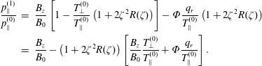 $$\begin{eqnarray}\displaystyle \frac{p_{\Vert }^{(1)}}{p_{\Vert }^{(0)}} & = & \displaystyle \frac{B_{z}}{B_{0}}\left[1-\frac{T_{\bot }^{(0)}}{T_{\Vert }^{(0)}}\left(1+2\unicode[STIX]{x1D701}^{2}R(\unicode[STIX]{x1D701})\right)\right]-\unicode[STIX]{x1D6F7}\frac{q_{r}}{T_{\Vert }^{(0)}}\left(1+2\unicode[STIX]{x1D701}^{2}R(\unicode[STIX]{x1D701})\right)\nonumber\\ \displaystyle & = & \displaystyle \frac{B_{z}}{B_{0}}-\left(1+2\unicode[STIX]{x1D701}^{2}R(\unicode[STIX]{x1D701})\right)\left[\frac{B_{z}}{B_{0}}\frac{T_{\bot }^{(0)}}{T_{\Vert }^{(0)}}+\unicode[STIX]{x1D6F7}\frac{q_{r}}{T_{\Vert }^{(0)}}\right].\end{eqnarray}$$
Parallel temperature
The parallel temperature calculates (linearizing
 $p_{\Vert }=T_{\Vert }n$
) as
$p_{\Vert }=T_{\Vert }n$
) as
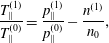 $$\begin{eqnarray}\frac{T_{\Vert }^{(1)}}{T_{\Vert }^{(0)}}=\frac{p_{\Vert }^{(1)}}{p_{\Vert }^{(0)}}-\frac{n^{(1)}}{n_{0}},\end{eqnarray}$$
that yields
 $$\begin{eqnarray}\displaystyle \frac{T_{\Vert }^{(1)}}{T_{\Vert }^{(0)}} & = & \displaystyle -\frac{B_{z}}{B_{0}}\frac{T_{\bot }^{(0)}}{T_{\Vert }^{(0)}}\left(1+2\unicode[STIX]{x1D701}^{2}R(\unicode[STIX]{x1D701})-R(\unicode[STIX]{x1D701})\right)-\unicode[STIX]{x1D6F7}\frac{q_{r}}{T_{\Vert }^{(0)}}\left(1+2\unicode[STIX]{x1D701}^{2}R(\unicode[STIX]{x1D701})-R(\unicode[STIX]{x1D701})\right)\nonumber\\ \displaystyle & = & \displaystyle -\left(1+2\unicode[STIX]{x1D701}^{2}R(\unicode[STIX]{x1D701})-R(\unicode[STIX]{x1D701})\right)\left[\frac{B_{z}}{B_{0}}\frac{T_{\bot }^{(0)}}{T_{\Vert }^{(0)}}+\unicode[STIX]{x1D6F7}\frac{q_{r}}{T_{\Vert }^{(0)}}\right].\end{eqnarray}$$
Perpendicular pressure
The perpendicular pressure calculates as
 $$\begin{eqnarray}\displaystyle p_{\bot }^{(1)} & = & \displaystyle \frac{m_{r}}{2}\frac{B_{z}}{B_{0}}\unicode[STIX]{x1D6FC}_{\bot }\left[\int v_{\bot }^{4}f_{0}\,\text{d}^{3}v+\frac{\unicode[STIX]{x1D6FC}_{\Vert }}{\unicode[STIX]{x1D6FC}_{\bot }}\int \frac{k_{\Vert }v_{\Vert }v_{\bot }^{4}}{(\unicode[STIX]{x1D714}-k_{\Vert }v_{\Vert })}f_{0}\,\text{d}^{3}v\right]\nonumber\\ \displaystyle & & \displaystyle +\,\frac{m_{r}}{2}\unicode[STIX]{x1D6F7}\frac{q_{r}}{m_{r}}2\unicode[STIX]{x1D6FC}_{\Vert }\int \frac{k_{\Vert }v_{\Vert }v_{\bot }^{2}}{(\unicode[STIX]{x1D714}-k_{\Vert }v_{\Vert })}f_{0}\,\text{d}^{3}v\nonumber\\ \displaystyle & = & \displaystyle \frac{m_{r}}{2}\frac{B_{z}}{B_{0}}\unicode[STIX]{x1D6FC}_{\bot }\left[n_{0}\frac{2}{\unicode[STIX]{x1D6FC}_{\bot }^{2}}+\frac{\unicode[STIX]{x1D6FC}_{\Vert }}{\unicode[STIX]{x1D6FC}_{\bot }}(-n_{0})R(\unicode[STIX]{x1D701})\frac{2}{\unicode[STIX]{x1D6FC}_{\bot }^{2}}\right]+\frac{m_{r}}{2}\unicode[STIX]{x1D6F7}\frac{q_{r}}{m_{r}}2\unicode[STIX]{x1D6FC}_{\Vert }(-n_{0})R(\unicode[STIX]{x1D701})\frac{1}{\unicode[STIX]{x1D6FC}_{\bot }},\nonumber\end{eqnarray}$$
so that
 $$\begin{eqnarray}\frac{p_{\bot }^{(1)}}{n_{0}}=m_{r}\frac{B_{z}}{B_{0}}\frac{1}{\unicode[STIX]{x1D6FC}_{\bot }}\left[1-\frac{\unicode[STIX]{x1D6FC}_{\Vert }}{\unicode[STIX]{x1D6FC}_{\bot }}R(\unicode[STIX]{x1D701})\right]-\unicode[STIX]{x1D6F7}q_{r}\frac{\unicode[STIX]{x1D6FC}_{\Vert }}{\unicode[STIX]{x1D6FC}_{\bot }}R(\unicode[STIX]{x1D701}),\end{eqnarray}$$
further yielding
 $$\begin{eqnarray}\frac{p_{\bot }^{(1)}}{p_{\bot }^{(0)}}=\frac{B_{z}}{B_{0}}2\left[1-\frac{T_{\bot }^{(0)}}{T_{\Vert }^{(0)}}R(\unicode[STIX]{x1D701})\right]-\unicode[STIX]{x1D6F7}\frac{q_{r}}{T_{\Vert }^{(0)}}R(\unicode[STIX]{x1D701}).\end{eqnarray}$$
Perpendicular temperature
The perpendicular temperature calculates (linearizing
 $p_{\bot }=T_{\bot }n$
) as
$p_{\bot }=T_{\bot }n$
) as
 $$\begin{eqnarray}\frac{T_{\bot }^{(1)}}{T_{\bot }^{(0)}}=\frac{p_{\bot }^{(1)}}{p_{\bot }^{(0)}}-\frac{n^{(1)}}{n_{0}},\end{eqnarray}$$
that yields
 $$\begin{eqnarray}\frac{T_{\bot }^{(1)}}{T_{\bot }^{(0)}}=\frac{B_{z}}{B_{0}}\left[1-\frac{T_{\bot }^{(0)}}{T_{\Vert }^{(0)}}R(\unicode[STIX]{x1D701})\right].\end{eqnarray}$$
We might be tired of calculations at this stage, but this result nicely shows that (at the linear level and at the long scales and low frequencies considered here) the Landau damping (
 ${\sim}E_{z}$
) does not influence the perpendicular temperature, however, the transit-time damping still does.
${\sim}E_{z}$
) does not influence the perpendicular temperature, however, the transit-time damping still does.
Parallel heat flux
The parallel heat flux calculates as
 $$\begin{eqnarray}\displaystyle q_{\Vert }^{(1)} & = & \displaystyle m_{r}\frac{B_{z}}{B_{0}}\unicode[STIX]{x1D6FC}_{\bot }\left[\underbrace{\int v_{\Vert }^{3}v_{\bot }^{2}f_{0}\,\text{d}^{3}v}_{=0}+\frac{\unicode[STIX]{x1D6FC}_{\Vert }}{\unicode[STIX]{x1D6FC}_{\bot }}\int \frac{k_{\Vert }v_{\Vert }^{4}v_{\bot }^{2}}{(\unicode[STIX]{x1D714}-k_{\Vert }v_{\Vert })}f_{0}\,\text{d}^{3}v\right]\nonumber\\ \displaystyle & & \displaystyle +\,m_{r}\unicode[STIX]{x1D6F7}\frac{q_{r}}{m_{r}}2\unicode[STIX]{x1D6FC}_{\Vert }\int \frac{k_{\Vert }v_{\Vert }^{4}}{(\unicode[STIX]{x1D714}-k_{\Vert }v_{\Vert })}f_{0}\,\text{d}^{3}v-3p_{\Vert }^{(0)}u_{\Vert }^{(1)}\nonumber\\ \displaystyle & = & \displaystyle -m_{r}\frac{B_{z}}{B_{0}}\unicode[STIX]{x1D6FC}_{\Vert }\frac{n_{0}}{\unicode[STIX]{x1D6FC}_{\Vert }^{3/2}}\text{sign}(k_{\Vert })\left(\frac{\unicode[STIX]{x1D701}}{2}+\unicode[STIX]{x1D701}^{3}R(\unicode[STIX]{x1D701})\right)\frac{1}{\unicode[STIX]{x1D6FC}_{\bot }}\nonumber\\ \displaystyle & & \displaystyle -\,m_{r}\unicode[STIX]{x1D6F7}\frac{q_{r}}{m_{r}}2\unicode[STIX]{x1D6FC}_{\Vert }\frac{n_{0}}{\unicode[STIX]{x1D6FC}_{\Vert }^{3/2}}\text{sign}(k_{\Vert })\left(\frac{\unicode[STIX]{x1D701}}{2}+\unicode[STIX]{x1D701}^{3}R(\unicode[STIX]{x1D701})\right)-3p_{\Vert }^{(0)}u_{\Vert }^{(1)}\nonumber\\ \displaystyle & = & \displaystyle -\frac{n_{0}m_{r}}{\unicode[STIX]{x1D6FC}_{\Vert }^{3/2}}\text{sign}(k_{\Vert })\left(\frac{\unicode[STIX]{x1D701}}{2}+\unicode[STIX]{x1D701}^{3}R(\unicode[STIX]{x1D701})\right)\left[\frac{B_{z}}{B_{0}}\frac{\unicode[STIX]{x1D6FC}_{\Vert }}{\unicode[STIX]{x1D6FC}_{\bot }}+\unicode[STIX]{x1D6F7}\frac{q_{r}}{m_{r}}2\unicode[STIX]{x1D6FC}_{\Vert }\right]-3p_{\Vert }^{(0)}u_{\Vert }^{(1)},\nonumber\end{eqnarray}$$
so that
 $$\begin{eqnarray}\displaystyle \frac{q_{\Vert }^{(1)}}{p_{\Vert }^{(0)}} & = & \displaystyle -\frac{1}{\sqrt{\unicode[STIX]{x1D6FC}_{\Vert }}}\text{sign}(k_{\Vert })\left(\unicode[STIX]{x1D701}+2\unicode[STIX]{x1D701}^{3}R(\unicode[STIX]{x1D701})\right)\left[\frac{B_{z}}{B_{0}}\frac{\unicode[STIX]{x1D6FC}_{\Vert }}{\unicode[STIX]{x1D6FC}_{\bot }}+\unicode[STIX]{x1D6F7}\frac{q_{r}}{m_{r}}2\unicode[STIX]{x1D6FC}_{\Vert }\right]-3u_{\Vert }^{(1)}\nonumber\\ \displaystyle & = & \displaystyle -\frac{1}{\sqrt{\unicode[STIX]{x1D6FC}_{\Vert }}}\text{sign}(k_{\Vert })\left(\unicode[STIX]{x1D701}+2\unicode[STIX]{x1D701}^{3}R(\unicode[STIX]{x1D701})-3\unicode[STIX]{x1D701}R(\unicode[STIX]{x1D701})\right)\left[\frac{B_{z}}{B_{0}}\frac{\unicode[STIX]{x1D6FC}_{\Vert }}{\unicode[STIX]{x1D6FC}_{\bot }}+\unicode[STIX]{x1D6F7}\frac{q_{r}}{m_{r}}2\unicode[STIX]{x1D6FC}_{\Vert }\right],\end{eqnarray}$$
or alternatively
 $$\begin{eqnarray}\displaystyle q_{\Vert }^{(1)}=-\sqrt{\frac{2T_{\Vert }^{(0)}}{m_{r}}}n_{0}T_{\Vert }^{(0)}\text{sign}(k_{\Vert })\left(\unicode[STIX]{x1D701}+2\unicode[STIX]{x1D701}^{3}R(\unicode[STIX]{x1D701})-3\unicode[STIX]{x1D701}R(\unicode[STIX]{x1D701})\right)\left[\frac{B_{z}}{B_{0}}\frac{T_{\bot }^{(0)}}{T_{\Vert }^{(0)}}+\unicode[STIX]{x1D6F7}\frac{q_{r}}{T_{\Vert }^{(0)}}\right]. & & \displaystyle\end{eqnarray}$$
Perpendicular heat flux
The perpendicular heat flux calculates as
 $$\begin{eqnarray}\displaystyle q_{\bot }^{(1)} & = & \displaystyle \frac{m_{r}}{2}\frac{B_{z}}{B_{0}}\unicode[STIX]{x1D6FC}_{\bot }\left[\underbrace{\int v_{\Vert }v_{\bot }^{4}f_{0}\,\text{d}^{3}v}_{=0}+\frac{\unicode[STIX]{x1D6FC}_{\Vert }}{\unicode[STIX]{x1D6FC}_{\bot }}\int \frac{k_{\Vert }v_{\Vert }^{2}v_{\bot }^{4}}{(\unicode[STIX]{x1D714}-k_{\Vert }v_{\Vert })}f_{0}\,\text{d}^{3}v\right]\nonumber\\ \displaystyle & & \displaystyle +\,\frac{m_{r}}{2}\unicode[STIX]{x1D6F7}\frac{q_{r}}{m_{r}}2\unicode[STIX]{x1D6FC}_{\Vert }\int \frac{k_{\Vert }v_{\Vert }^{2}v_{\bot }^{2}}{(\unicode[STIX]{x1D714}-k_{\Vert }v_{\Vert })}f_{0}\,\text{d}^{3}v-p_{\bot }^{(0)}u_{\Vert }^{(1)}\nonumber\\ \displaystyle & = & \displaystyle -\frac{m_{r}}{2}\frac{B_{z}}{B_{0}}\unicode[STIX]{x1D6FC}_{\Vert }n_{0}\frac{1}{\sqrt{\unicode[STIX]{x1D6FC}_{\Vert }}}\text{sign}(k_{\Vert })\unicode[STIX]{x1D701}R(\unicode[STIX]{x1D701})\frac{2}{\unicode[STIX]{x1D6FC}_{\bot }^{2}}\nonumber\\ \displaystyle & & \displaystyle -\,\frac{m_{r}}{2}\unicode[STIX]{x1D6F7}\frac{q_{r}}{m_{r}}2\unicode[STIX]{x1D6FC}_{\Vert }n_{0}\frac{1}{\sqrt{\unicode[STIX]{x1D6FC}_{\Vert }}}\text{sign}(k_{\Vert })\unicode[STIX]{x1D701}R(\unicode[STIX]{x1D701})\frac{1}{\unicode[STIX]{x1D6FC}_{\bot }}-p_{\bot }^{(0)}u_{\Vert }^{(1)}\nonumber\\ \displaystyle & = & \displaystyle -\frac{m_{r}}{2}\frac{n_{0}}{\sqrt{\unicode[STIX]{x1D6FC}_{\Vert }}}\text{sign}(k_{\Vert })\unicode[STIX]{x1D701}R(\unicode[STIX]{x1D701})\frac{1}{\unicode[STIX]{x1D6FC}_{\bot }}\left[\frac{B_{z}}{B_{0}}\frac{2\unicode[STIX]{x1D6FC}_{\Vert }}{\unicode[STIX]{x1D6FC}_{\bot }}+\unicode[STIX]{x1D6F7}\frac{q_{r}}{m_{r}}2\unicode[STIX]{x1D6FC}_{\Vert }\right]-p_{\bot }^{(0)}u_{\Vert }^{(1)},\nonumber\end{eqnarray}$$
so that
 $$\begin{eqnarray}\displaystyle \frac{q_{\bot }^{(1)}}{p_{\bot }^{(0)}} & = & \displaystyle -\frac{1}{\sqrt{\unicode[STIX]{x1D6FC}_{\Vert }}}\text{sign}(k_{\Vert })\unicode[STIX]{x1D701}R(\unicode[STIX]{x1D701})\left[\frac{B_{z}}{B_{0}}\frac{2\unicode[STIX]{x1D6FC}_{\Vert }}{\unicode[STIX]{x1D6FC}_{\bot }}+\unicode[STIX]{x1D6F7}\frac{q_{r}}{m_{r}}2\unicode[STIX]{x1D6FC}_{\Vert }\right]-u_{\Vert }^{(1)}\nonumber\\ \displaystyle & = & \displaystyle -\frac{1}{\sqrt{\unicode[STIX]{x1D6FC}_{\Vert }}}\text{sign}(k_{\Vert })\unicode[STIX]{x1D701}R(\unicode[STIX]{x1D701})\frac{B_{z}}{B_{0}}\frac{\unicode[STIX]{x1D6FC}_{\Vert }}{\unicode[STIX]{x1D6FC}_{\bot }},\end{eqnarray}$$
or alternatively
 $$\begin{eqnarray}q_{\bot }^{(1)}=-\sqrt{\frac{2T_{\Vert }^{(0)}}{m_{r}}}p_{\bot }^{(0)}\frac{T_{\bot }^{(0)}}{T_{\Vert }^{(0)}}\text{sign}(k_{\Vert })\unicode[STIX]{x1D701}R(\unicode[STIX]{x1D701})\frac{B_{z}}{B_{0}}.\end{eqnarray}$$
The perpendicular heat flux
 $q_{\bot }^{(1)}$
(similarly to the perpendicular temperature
$q_{\bot }^{(1)}$
(similarly to the perpendicular temperature
 $T_{\bot }^{(1)}$
), is also not directly influenced by the Landau damping
$T_{\bot }^{(1)}$
), is also not directly influenced by the Landau damping
 $({\sim}E_{z})$
, even though it is influenced by the transit-time damping
$({\sim}E_{z})$
, even though it is influenced by the transit-time damping
 $({\sim}B_{z})$
.
$({\sim}B_{z})$
.
Fourth-order moment
$r_{\Vert \Vert }$

The fourth-order moment
 $r_{\Vert \Vert }$
calculates as
$r_{\Vert \Vert }$
calculates as
 $$\begin{eqnarray}\displaystyle r_{\Vert \Vert }^{(1)} & = & \displaystyle m_{r}\frac{B_{z}}{B_{0}}\unicode[STIX]{x1D6FC}_{\bot }\left[\int v_{\Vert }^{4}v_{\bot }^{2}f_{0}\,\text{d}^{3}v+\frac{\unicode[STIX]{x1D6FC}_{\Vert }}{\unicode[STIX]{x1D6FC}_{\bot }}\int \frac{k_{\Vert }v_{\Vert }^{5}v_{\bot }^{2}}{(\unicode[STIX]{x1D714}-k_{\Vert }v_{\Vert })}f_{0}\,\text{d}^{3}v\right]\nonumber\\ \displaystyle & & \displaystyle +\,m_{r}\unicode[STIX]{x1D6F7}\frac{q_{r}}{m_{r}}2\unicode[STIX]{x1D6FC}_{\Vert }\int \frac{k_{\Vert }v_{\Vert }^{5}}{(\unicode[STIX]{x1D714}-k_{\Vert }v_{\Vert })}f_{0}\,\text{d}^{3}v\nonumber\\ \displaystyle & = & \displaystyle m_{r}\frac{B_{z}}{B_{0}}\unicode[STIX]{x1D6FC}_{\bot }\left[n_{0}\frac{3}{4\unicode[STIX]{x1D6FC}_{\Vert }^{2}\unicode[STIX]{x1D6FC}_{\bot }}+\frac{\unicode[STIX]{x1D6FC}_{\Vert }}{\unicode[STIX]{x1D6FC}_{\bot }}\frac{(-n_{0})}{\unicode[STIX]{x1D6FC}_{\Vert }^{2}}\left(\frac{3}{4}+\frac{\unicode[STIX]{x1D701}^{2}}{2}+\unicode[STIX]{x1D701}^{4}R(\unicode[STIX]{x1D701})\right)\frac{1}{\unicode[STIX]{x1D6FC}_{\bot }}\right]\nonumber\\ \displaystyle & & \displaystyle +\,m_{r}\unicode[STIX]{x1D6F7}\frac{q_{r}}{m_{r}}2\unicode[STIX]{x1D6FC}_{\Vert }\frac{(-n_{0})}{\unicode[STIX]{x1D6FC}_{\Vert }^{2}}\left(\frac{3}{4}+\frac{\unicode[STIX]{x1D701}^{2}}{2}+\unicode[STIX]{x1D701}^{4}R(\unicode[STIX]{x1D701})\right)\nonumber\\ \displaystyle & = & \displaystyle m_{r}\frac{B_{z}}{B_{0}}n_{0}\frac{3}{4\unicode[STIX]{x1D6FC}_{\Vert }^{2}}-m_{r}n_{0}\left(\frac{3}{4}+\frac{\unicode[STIX]{x1D701}^{2}}{2}+\unicode[STIX]{x1D701}^{4}R(\unicode[STIX]{x1D701})\right)\frac{1}{\unicode[STIX]{x1D6FC}_{\Vert }^{2}}\left[\frac{B_{z}}{B_{0}}\frac{\unicode[STIX]{x1D6FC}_{\Vert }}{\unicode[STIX]{x1D6FC}_{\bot }}+\unicode[STIX]{x1D6F7}\frac{q_{r}}{m_{r}}2\unicode[STIX]{x1D6FC}_{\Vert }\right],\end{eqnarray}$$
so that
 $$\begin{eqnarray}\displaystyle r_{\Vert \Vert }^{(1)}=\frac{p_{\Vert }^{(0)}T_{\Vert }^{(0)}}{m_{r}}\left\{3\frac{B_{z}}{B_{0}}-\left(3+2\unicode[STIX]{x1D701}^{2}+4\unicode[STIX]{x1D701}^{4}R(\unicode[STIX]{x1D701})\right)\left[\frac{B_{z}}{B_{0}}\frac{T_{\bot }^{(0)}}{T_{\Vert }^{(0)}}+\unicode[STIX]{x1D6F7}\frac{q_{r}}{T_{\Vert }^{(0)}}\right]\right\}. & & \displaystyle\end{eqnarray}$$
Fourth-order moment deviation
$\widetilde{r}_{\Vert \Vert }$

The fourth-order moment ‘deviation’
 $\widetilde{r}_{\Vert \Vert }^{(1)}$
calculates as (linearizing
$\widetilde{r}_{\Vert \Vert }^{(1)}$
calculates as (linearizing
 $r_{\Vert \Vert }=(3/m_{r})p_{\Vert }T_{\Vert }+\widetilde{r}_{\Vert \Vert }$
with definitions
$r_{\Vert \Vert }=(3/m_{r})p_{\Vert }T_{\Vert }+\widetilde{r}_{\Vert \Vert }$
with definitions
 $r_{\Vert \Vert }^{(0)}=(3/m_{r})p_{\Vert }^{(0)}T_{\Vert }^{(0)}$
and
$r_{\Vert \Vert }^{(0)}=(3/m_{r})p_{\Vert }^{(0)}T_{\Vert }^{(0)}$
and
 $\widetilde{r}_{\Vert \Vert }^{(0)}=0$
)
$\widetilde{r}_{\Vert \Vert }^{(0)}=0$
)
 $$\begin{eqnarray}\frac{r_{\Vert \Vert }^{(1)}}{r_{\Vert \Vert }^{(0)}}=\frac{p_{\Vert }^{(1)}}{p_{\Vert }^{(0)}}+\frac{T_{\Vert }^{(1)}}{T_{\Vert }^{(0)}}+\frac{\widetilde{r}_{\Vert \Vert }^{(1)}}{r_{\Vert \Vert }^{(0)}},\end{eqnarray}$$
or equivalently
 $$\begin{eqnarray}\widetilde{r}_{\Vert \Vert }^{(1)}=r_{\Vert \Vert }^{(1)}-\frac{3}{m_{r}}p_{\Vert }^{(0)}T_{\Vert }^{(0)}\left(\frac{p_{\Vert }^{(1)}}{p_{\Vert }^{(0)}}+\frac{T_{\Vert }^{(1)}}{T_{\Vert }^{(0)}}\right),\end{eqnarray}$$
which yields
 $$\begin{eqnarray}\widetilde{r}_{\Vert \Vert }^{(1)}=-\frac{p_{\Vert }^{(0)}T_{\Vert }^{(0)}}{m_{r}}\left(2\unicode[STIX]{x1D701}^{2}+4\unicode[STIX]{x1D701}^{4}R(\unicode[STIX]{x1D701})+3R(\unicode[STIX]{x1D701})-3-12\unicode[STIX]{x1D701}^{2}R(\unicode[STIX]{x1D701})\right)\left[\frac{B_{z}}{B_{0}}\frac{T_{\bot }^{(0)}}{T_{\Vert }^{(0)}}+\unicode[STIX]{x1D6F7}\frac{q_{r}}{T_{\Vert }^{(0)}}\right].\end{eqnarray}$$
Fourth-order moment
$r_{\Vert \bot }$

The fourth-order moment
 $r_{\Vert \bot }$
calculates as
$r_{\Vert \bot }$
calculates as
 $$\begin{eqnarray}\displaystyle r_{\Vert \bot }^{(1)} & = & \displaystyle \frac{m_{r}}{2}\frac{B_{z}}{B_{0}}\unicode[STIX]{x1D6FC}_{\bot }\left[\int v_{\Vert }^{2}v_{\bot }^{4}f_{0}\,\text{d}^{3}v+\frac{\unicode[STIX]{x1D6FC}_{\Vert }}{\unicode[STIX]{x1D6FC}_{\bot }}\int \frac{k_{\Vert }v_{\Vert }^{3}v_{\bot }^{4}}{(\unicode[STIX]{x1D714}-k_{\Vert }v_{\Vert })}f_{0}\,\text{d}^{3}v\right]\nonumber\\ \displaystyle & & \displaystyle +\,\frac{m_{r}}{2}\unicode[STIX]{x1D6F7}\frac{q_{r}}{m_{r}}2\unicode[STIX]{x1D6FC}_{\Vert }\int \frac{k_{\Vert }v_{\Vert }^{3}v_{\bot }^{2}}{(\unicode[STIX]{x1D714}-k_{\Vert }v_{\Vert })}f_{0}\,\text{d}^{3}v\nonumber\\ \displaystyle & = & \displaystyle \frac{m_{r}}{2}\frac{B_{z}}{B_{0}}\unicode[STIX]{x1D6FC}_{\bot }\left[\frac{n_{0}}{\unicode[STIX]{x1D6FC}_{\Vert }\unicode[STIX]{x1D6FC}_{\bot }^{2}}-\frac{\unicode[STIX]{x1D6FC}_{\Vert }}{\unicode[STIX]{x1D6FC}_{\bot }}n_{0}\frac{2}{\unicode[STIX]{x1D6FC}_{\Vert }\unicode[STIX]{x1D6FC}_{\bot }^{2}}\left(\frac{1}{2}+\unicode[STIX]{x1D701}^{2}R(\unicode[STIX]{x1D701})\right)\right]\nonumber\\ \displaystyle & & \displaystyle -\,\frac{m_{r}}{2}\unicode[STIX]{x1D6F7}\frac{q_{r}}{m_{r}}2\unicode[STIX]{x1D6FC}_{\Vert }\frac{n_{0}}{\unicode[STIX]{x1D6FC}_{\Vert }\unicode[STIX]{x1D6FC}_{\bot }}\left(\frac{1}{2}+\unicode[STIX]{x1D701}^{2}R(\unicode[STIX]{x1D701})\right)\nonumber\\ \displaystyle & = & \displaystyle \frac{m_{r}}{2}\frac{B_{z}}{B_{0}}\frac{n_{0}}{\unicode[STIX]{x1D6FC}_{\Vert }\unicode[STIX]{x1D6FC}_{\bot }}-m_{r}n_{0}\left(\frac{1}{2}+\unicode[STIX]{x1D701}^{2}R(\unicode[STIX]{x1D701})\right)\frac{1}{\unicode[STIX]{x1D6FC}_{\Vert }\unicode[STIX]{x1D6FC}_{\bot }}\left[\frac{B_{z}}{B_{0}}\frac{\unicode[STIX]{x1D6FC}_{\Vert }}{\unicode[STIX]{x1D6FC}_{\bot }}+\frac{1}{2}\unicode[STIX]{x1D6F7}\frac{q_{r}}{m_{r}}2\unicode[STIX]{x1D6FC}_{\Vert }\right],\end{eqnarray}$$
so that
 $$\begin{eqnarray}\displaystyle r_{\Vert \bot }^{(1)}=\frac{p_{\Vert }^{(0)}T_{\bot }^{(0)}}{m_{r}}\left\{2\frac{B_{z}}{B_{0}}-\left(2+4\unicode[STIX]{x1D701}^{2}R(\unicode[STIX]{x1D701})\right)\left[\frac{B_{z}}{B_{0}}\frac{T_{\bot }^{(0)}}{T_{\Vert }^{(0)}}+\frac{1}{2}\unicode[STIX]{x1D6F7}\frac{q_{r}}{T_{\Vert }^{(0)}}\right]\right\}. & & \displaystyle\end{eqnarray}$$
Fourth-order moment deviation
$\widetilde{r}_{\Vert \bot }$

The fourth-order moment ‘deviation’
 $\widetilde{r}_{\Vert \bot }^{(1)}$
calculates as (for example linearizing
$\widetilde{r}_{\Vert \bot }^{(1)}$
calculates as (for example linearizing
 $r_{\Vert \bot }=(1/m_{r})p_{\Vert }T_{\bot }+\widetilde{r}_{\Vert \bot }$
with definitions
$r_{\Vert \bot }=(1/m_{r})p_{\Vert }T_{\bot }+\widetilde{r}_{\Vert \bot }$
with definitions
 $r_{\Vert \bot }^{(0)}=(1/m_{r})p_{\Vert }^{(0)}T_{\bot }^{(0)}$
and
$r_{\Vert \bot }^{(0)}=(1/m_{r})p_{\Vert }^{(0)}T_{\bot }^{(0)}$
and
 $\widetilde{r}_{\Vert \bot }^{(0)}=0$
)
$\widetilde{r}_{\Vert \bot }^{(0)}=0$
)
 $$\begin{eqnarray}\frac{r_{\Vert \bot }^{(1)}}{r_{\Vert \bot }^{(0)}}=\frac{p_{\Vert }^{(1)}}{p_{\Vert }^{(0)}}+\frac{T_{\bot }^{(1)}}{T_{\bot }^{(0)}}+\frac{\widetilde{r}_{\Vert \bot }^{(1)}}{r_{\Vert \bot }^{(0)}},\end{eqnarray}$$
or equivalently
 $$\begin{eqnarray}\widetilde{r}_{\Vert \bot }^{(1)}=r_{\Vert \bot }^{(1)}-\frac{1}{m_{r}}p_{\Vert }^{(0)}T_{\bot }^{(0)}\left(\frac{p_{\Vert }^{(1)}}{p_{\Vert }^{(0)}}+\frac{T_{\bot }^{(1)}}{T_{\bot }^{(0)}}\right),\end{eqnarray}$$
and the result is
 $$\begin{eqnarray}\widetilde{r}_{\Vert \bot }^{(1)}=-\frac{p_{\bot }^{(0)}T_{\bot }^{(0)}}{m_{r}}\frac{B_{z}}{B_{0}}\left(1+2\unicode[STIX]{x1D701}^{2}R(\unicode[STIX]{x1D701})-R(\unicode[STIX]{x1D701})\right).\end{eqnarray}$$
Fourth-order moment
$r_{\bot \bot }$

The fourth-order moment
 $r_{\bot \bot }$
calculates as
$r_{\bot \bot }$
calculates as
 $$\begin{eqnarray}\displaystyle r_{\bot \bot }^{(1)} & = & \displaystyle \frac{m_{r}}{4}\frac{B_{z}}{B_{0}}\unicode[STIX]{x1D6FC}_{\bot }\left[\int v_{\bot }^{6}f_{0}\,\text{d}^{3}v+\frac{\unicode[STIX]{x1D6FC}_{\Vert }}{\unicode[STIX]{x1D6FC}_{\bot }}\int \frac{k_{\Vert }v_{\Vert }v_{\bot }^{6}}{(\unicode[STIX]{x1D714}-k_{\Vert }v_{\Vert })}f_{0}\,\text{d}^{3}v\right]\nonumber\\ \displaystyle & & \displaystyle +\,\frac{m_{r}}{4}\unicode[STIX]{x1D6F7}\frac{q_{r}}{m_{r}}2\unicode[STIX]{x1D6FC}_{\Vert }\int \frac{k_{\Vert }v_{\Vert }v_{\bot }^{4}}{(\unicode[STIX]{x1D714}-k_{\Vert }v_{\Vert })}f_{0}\,\text{d}^{3}v\nonumber\\ \displaystyle & = & \displaystyle \frac{m_{r}}{4}\frac{B_{z}}{B_{0}}\unicode[STIX]{x1D6FC}_{\bot }\left[n_{0}\frac{6}{\unicode[STIX]{x1D6FC}_{\bot }^{3}}-\frac{\unicode[STIX]{x1D6FC}_{\Vert }}{\unicode[STIX]{x1D6FC}_{\bot }}n_{0}R(\unicode[STIX]{x1D701})\frac{6}{\unicode[STIX]{x1D6FC}_{\bot }^{3}}\right]-\frac{m_{r}}{4}\unicode[STIX]{x1D6F7}\frac{q_{r}}{m_{r}}2\unicode[STIX]{x1D6FC}_{\Vert }n_{0}R(\unicode[STIX]{x1D701})\frac{2}{\unicode[STIX]{x1D6FC}_{\bot }^{2}},\end{eqnarray}$$
and the result is
 $$\begin{eqnarray}r_{\bot \bot }^{(1)}=\frac{2p_{\bot }^{(0)}T_{\bot }^{(0)}}{m_{r}}\left\{3\frac{B_{z}}{B_{0}}\left(1-\frac{T_{\bot }^{(0)}}{T_{\Vert }^{(0)}}R(\unicode[STIX]{x1D701})\right)-\unicode[STIX]{x1D6F7}\frac{q_{r}}{T_{\Vert }^{(0)}}R(\unicode[STIX]{x1D701})\right\}.\end{eqnarray}$$
Fourth-order moment deviation
$\widetilde{r}_{\bot \bot }$

The fourth-order moment deviation
 $\widetilde{r}_{\bot \bot }^{(1)}$
calculates as (for example linearizing
$\widetilde{r}_{\bot \bot }^{(1)}$
calculates as (for example linearizing
 $r_{\bot \bot }=(2/m_{r})p_{\bot }T_{\bot }+\widetilde{r}_{\bot \bot }$
with definitions
$r_{\bot \bot }=(2/m_{r})p_{\bot }T_{\bot }+\widetilde{r}_{\bot \bot }$
with definitions
 $r_{\bot \bot }^{(0)}=(2/m_{r})p_{\bot }^{(0)}T_{\bot }^{(0)}$
and
$r_{\bot \bot }^{(0)}=(2/m_{r})p_{\bot }^{(0)}T_{\bot }^{(0)}$
and
 $\widetilde{r}_{\bot \bot }^{(0)}=0$
)
$\widetilde{r}_{\bot \bot }^{(0)}=0$
)
 $$\begin{eqnarray}\frac{r_{\bot \bot }^{(1)}}{r_{\bot \bot }^{(0)}}=\frac{p_{\bot }^{(1)}}{p_{\bot }^{(0)}}+\frac{T_{\bot }^{(1)}}{T_{\bot }^{(0)}}+\frac{\widetilde{r}_{\bot \bot }^{(1)}}{r_{\bot \bot }^{(0)}},\end{eqnarray}$$
or equivalently
 $$\begin{eqnarray}\widetilde{r}_{\bot \bot }^{(1)}=r_{\bot \bot }^{(1)}-\frac{2p_{\bot }^{(0)}T_{\bot }^{(0)}}{m_{r}}\left(\frac{p_{\bot }^{(1)}}{p_{\bot }^{(0)}}+\frac{T_{\bot }^{(1)}}{T_{\bot }^{(0)}}\right),\end{eqnarray}$$
which yields
 $$\begin{eqnarray}\widetilde{r}_{\bot \bot }^{(1)}=0.\end{eqnarray}$$
This is excellent news, since we will not have to consider closures for
 $\widetilde{r}_{\bot \bot }^{(1)}$
.
$\widetilde{r}_{\bot \bot }^{(1)}$
.
4.4 Landau fluid closures in three dimensions
Let us separate the kinetic moments into two groups. The first group
 $$\begin{eqnarray}\displaystyle u_{\Vert }^{(1)} & = & \displaystyle -\sqrt{\frac{2T_{\Vert }^{(0)}}{m_{r}}}\text{sign}(k_{\Vert })\unicode[STIX]{x1D701}R(\unicode[STIX]{x1D701})\left[\frac{B_{z}}{B_{0}}\frac{T_{\bot }^{(0)}}{T_{\Vert }^{(0)}}+\unicode[STIX]{x1D6F7}\frac{q_{r}}{T_{\Vert }^{(0)}}\right];\end{eqnarray}$$
 $$\begin{eqnarray}\displaystyle \frac{T_{\Vert }^{(1)}}{T_{\Vert }^{(0)}} & = & \displaystyle -\left(1+2\unicode[STIX]{x1D701}^{2}R(\unicode[STIX]{x1D701})-R(\unicode[STIX]{x1D701})\right)\left[\frac{B_{z}}{B_{0}}\frac{T_{\bot }^{(0)}}{T_{\Vert }^{(0)}}+\unicode[STIX]{x1D6F7}\frac{q_{r}}{T_{\Vert }^{(0)}}\right];\end{eqnarray}$$
 $$\begin{eqnarray}\displaystyle q_{\Vert }^{(1)} & = & \displaystyle -\sqrt{\frac{2T_{\Vert }^{(0)}}{m_{r}}}n_{0}T_{\Vert }^{(0)}\text{sign}(k_{\Vert })\left(\unicode[STIX]{x1D701}+2\unicode[STIX]{x1D701}^{3}R(\unicode[STIX]{x1D701})-3\unicode[STIX]{x1D701}R(\unicode[STIX]{x1D701})\right)\left[\frac{B_{z}}{B_{0}}\frac{T_{\bot }^{(0)}}{T_{\Vert }^{(0)}}+\unicode[STIX]{x1D6F7}\frac{q_{r}}{T_{\Vert }^{(0)}}\right];\nonumber\\ \displaystyle & & \displaystyle\end{eqnarray}$$
 $$\begin{eqnarray}\displaystyle \widetilde{r}_{\Vert \Vert }^{(1)} & = & \displaystyle -\frac{p_{\Vert }^{(0)}T_{\Vert }^{(0)}}{m_{r}}\left(2\unicode[STIX]{x1D701}^{2}+4\unicode[STIX]{x1D701}^{4}R(\unicode[STIX]{x1D701})+3R(\unicode[STIX]{x1D701})-3-12\unicode[STIX]{x1D701}^{2}R(\unicode[STIX]{x1D701})\right)\left[\frac{B_{z}}{B_{0}}\frac{T_{\bot }^{(0)}}{T_{\Vert }^{(0)}}+\unicode[STIX]{x1D6F7}\frac{q_{r}}{T_{\Vert }^{(0)}}\right].\nonumber\\ \displaystyle & & \displaystyle\end{eqnarray}$$
And the second group
 $$\begin{eqnarray}\displaystyle \frac{T_{\bot }^{(1)}}{T_{\bot }^{(0)}} & = & \displaystyle \left[1-\frac{T_{\bot }^{(0)}}{T_{\Vert }^{(0)}}R(\unicode[STIX]{x1D701})\right]\frac{B_{z}}{B_{0}};\end{eqnarray}$$
 $$\begin{eqnarray}\displaystyle q_{\bot }^{(1)} & = & \displaystyle -\sqrt{\frac{2T_{\Vert }^{(0)}}{m_{r}}}p_{\bot }^{(0)}\frac{T_{\bot }^{(0)}}{T_{\Vert }^{(0)}}\text{sign}(k_{\Vert })\unicode[STIX]{x1D701}R(\unicode[STIX]{x1D701})\frac{B_{z}}{B_{0}};\end{eqnarray}$$
 $$\begin{eqnarray}\displaystyle \widetilde{r}_{\Vert \bot }^{(1)} & = & \displaystyle -\frac{p_{\bot }^{(0)}T_{\bot }^{(0)}}{m_{r}}\left(1+2\unicode[STIX]{x1D701}^{2}R(\unicode[STIX]{x1D701})-R(\unicode[STIX]{x1D701})\right)\frac{B_{z}}{B_{0}}.\end{eqnarray}$$
One immediately notices that the moments in the first group, are extremely similar to the moments we obtained in the simplified case of a 1-D geometry, where we neglected the transit-time damping, i.e. in the system (3.20)–(3.26). In fact, the system is completely the same, if the variable
 $(B_{z}/B_{0})(T_{\bot }^{(0)}/T_{\Vert }^{(0)})+\unicode[STIX]{x1D6F7}(q_{r}/T_{\Vert }^{(0)})$
is replaced by
$(B_{z}/B_{0})(T_{\bot }^{(0)}/T_{\Vert }^{(0)})+\unicode[STIX]{x1D6F7}(q_{r}/T_{\Vert }^{(0)})$
is replaced by
 $\unicode[STIX]{x1D6F7}(q_{r}/T_{\Vert }^{(0)})$
. Therefore, there is nothing more we can do here, and all the discussion and closures from the 1-D geometry, apply here in the 3-D geometry to closures for
$\unicode[STIX]{x1D6F7}(q_{r}/T_{\Vert }^{(0)})$
. Therefore, there is nothing more we can do here, and all the discussion and closures from the 1-D geometry, apply here in the 3-D geometry to closures for
 $q_{\Vert }^{(1)}$
and
$q_{\Vert }^{(1)}$
and
 $\widetilde{r}_{\Vert \Vert }^{(1)}$
without any changes. So for example,
$\widetilde{r}_{\Vert \Vert }^{(1)}$
without any changes. So for example,
 $$\begin{eqnarray}\displaystyle & \displaystyle R_{3,2}(\unicode[STIX]{x1D701}):\quad q_{\Vert }^{(1)}=-\frac{2}{\sqrt{\unicode[STIX]{x03C0}}}n_{0}v_{\text{th}\Vert }i\text{sign}(k_{\Vert })T_{\Vert }^{(1)}; & \displaystyle\end{eqnarray}$$
 $$\begin{eqnarray}\displaystyle & \displaystyle R_{4,3}(\unicode[STIX]{x1D701}):\quad \widetilde{r}_{\Vert \Vert }^{(1)}=-\frac{2\sqrt{\unicode[STIX]{x03C0}}}{(3\unicode[STIX]{x03C0}-8)}v_{\text{th}\Vert }i\text{sign}(k_{\Vert })q_{\Vert }^{(1)}+\frac{(32-9\unicode[STIX]{x03C0})}{2(3\unicode[STIX]{x03C0}-8)}v_{\text{th}\Vert }^{2}n_{0}T_{\Vert }^{(1)}, & \displaystyle\end{eqnarray}$$
and similarly for all the other closures that we considered in the 1-D geometry.
4.4.1 Closures for
$q_{\bot }$
and
$\widetilde{r}_{\Vert \bot }$


For the second group, we do not have many choices and the calculations are simpler. In comparison to the first group, the expressions for
 $q_{\bot }^{(1)}$
and
$q_{\bot }^{(1)}$
and
 $\widetilde{r}_{\Vert \bot }^{(1)}$
contain only powers
$\widetilde{r}_{\Vert \bot }^{(1)}$
contain only powers
 $\unicode[STIX]{x1D701}$
and
$\unicode[STIX]{x1D701}$
and
 $\unicode[STIX]{x1D701}^{2}$
. On one hand, this is good news since the analytic calculations are simpler and we will explore all possible cases of closure very quickly. On the other hand, this means that we will be able to use only relatively low-order Padé approximants to
$\unicode[STIX]{x1D701}^{2}$
. On one hand, this is good news since the analytic calculations are simpler and we will explore all possible cases of closure very quickly. On the other hand, this means that we will be able to use only relatively low-order Padé approximants to
 $R(\unicode[STIX]{x1D701})$
, implying that the closures will be less accurate.
$R(\unicode[STIX]{x1D701})$
, implying that the closures will be less accurate.
To easily spot closures, it is perhaps beneficial to use
 $$\begin{eqnarray}v_{\text{th}\Vert }=\sqrt{\frac{2T_{\Vert }^{(0)}}{m_{r}}};\quad a_{p}=\frac{T_{\bot }^{(0)}}{T_{\Vert }^{(0)}};\quad \widetilde{B}_{z}=\frac{B_{z}}{B_{0}},\end{eqnarray}$$
and the moments read
 $$\begin{eqnarray}\displaystyle \frac{T_{\bot }^{(1)}}{T_{\bot }^{(0)}} & = & \displaystyle \widetilde{B}_{z}\left[1-a_{p}R(\unicode[STIX]{x1D701})\right];\end{eqnarray}$$
 $$\begin{eqnarray}\displaystyle q_{\bot }^{(1)} & = & \displaystyle -v_{\text{th}\Vert }p_{\bot }^{(0)}a_{p}\text{sign}(k_{\Vert })\widetilde{B}_{z}\left[\unicode[STIX]{x1D701}R(\unicode[STIX]{x1D701})\right];\end{eqnarray}$$
 $$\begin{eqnarray}\displaystyle \widetilde{r}_{\Vert \bot }^{(1)} & = & \displaystyle -v_{\text{th}\Vert }^{2}p_{\bot }^{(0)}\frac{a_{p}}{2}\widetilde{B}_{z}\left[1+2\unicode[STIX]{x1D701}^{2}R(\unicode[STIX]{x1D701})-R(\unicode[STIX]{x1D701})\right].\end{eqnarray}$$
Before proceeding with Padé approximants, it is very beneficial to briefly consider the limit
 $\unicode[STIX]{x1D701}\ll 1$
, where
$\unicode[STIX]{x1D701}\ll 1$
, where
 $R(\unicode[STIX]{x1D701})\rightarrow 1$
. And a problem is immediately apparent. The quantities
$R(\unicode[STIX]{x1D701})\rightarrow 1$
. And a problem is immediately apparent. The quantities
 $q_{\bot }^{(1)}$
and
$q_{\bot }^{(1)}$
and
 $\widetilde{r}_{\Vert \bot }^{(1)}$
are small and converge to zero, however, this is in general not true for the perpendicular temperature
$\widetilde{r}_{\Vert \bot }^{(1)}$
are small and converge to zero, however, this is in general not true for the perpendicular temperature
 $T_{\bot }^{(1)}$
, where the result depends on the temperature anisotropy ratio
$T_{\bot }^{(1)}$
, where the result depends on the temperature anisotropy ratio
 $a_{p}$
. With anisotropic mean temperatures (
$a_{p}$
. With anisotropic mean temperatures (
 $a_{p}\neq 1$
), the quantity
$a_{p}\neq 1$
), the quantity
 $T_{\bot }^{(1)}$
will remain finite and will not converge to zero due to coupling with magnetic field perturbations
$T_{\bot }^{(1)}$
will remain finite and will not converge to zero due to coupling with magnetic field perturbations
 $B_{z}$
, essentially because of conservation of the magnetic moment. The quantity
$B_{z}$
, essentially because of conservation of the magnetic moment. The quantity
 $T_{\bot }^{(1)}$
, at least as it is written now, is therefore not suitable for the construction of closures. Or in another words, the technique with Padé approximants of
$T_{\bot }^{(1)}$
, at least as it is written now, is therefore not suitable for the construction of closures. Or in another words, the technique with Padé approximants of
 $R(\unicode[STIX]{x1D701})$
will not work, since the technique is based on matching the expressions for all
$R(\unicode[STIX]{x1D701})$
will not work, since the technique is based on matching the expressions for all
 $\unicode[STIX]{x1D701}$
values. To consider closures, we have to separate this finite contribution, so that the Padé technique can be used, i.e. by writing
$\unicode[STIX]{x1D701}$
values. To consider closures, we have to separate this finite contribution, so that the Padé technique can be used, i.e. by writing
 $$\begin{eqnarray}\displaystyle \frac{T_{\bot }^{(1)}}{T_{\bot }^{(0)}}=\widetilde{B}_{z}\left[1-a_{p}+a_{p}-a_{p}R(\unicode[STIX]{x1D701})\right]=\widetilde{B}_{z}(1-a_{p})+\widetilde{B}_{z}a_{p}\left[1-R(\unicode[STIX]{x1D701})\right], & & \displaystyle\end{eqnarray}$$
and by moving the finite contribution to the left-hand side
 $$\begin{eqnarray}\displaystyle \underbrace{\frac{T_{\bot }^{(1)}}{T_{\bot }^{(0)}}+\widetilde{B}_{z}(a_{p}-1)}_{={\mathcal{T}}_{\bot }} & = & \displaystyle \widetilde{B}_{z}a_{p}\left[1-R(\unicode[STIX]{x1D701})\right].\end{eqnarray}$$
Therefore, instead of looking for closures with
 $T_{\bot }^{(1)}$
, we have to look for closures with a quantity that is proportional to the left-hand side of this equation, that we call
$T_{\bot }^{(1)}$
, we have to look for closures with a quantity that is proportional to the left-hand side of this equation, that we call
 ${\mathcal{T}}_{\bot }$
(T written with the ‘mathcal’ command in latex), and for clarity written with the full notation
${\mathcal{T}}_{\bot }$
(T written with the ‘mathcal’ command in latex), and for clarity written with the full notation

where on the left is the definition of the new quantity, and on the right is the kinetic moment that this new quantity satisfies. Only now we are ready to use the Padé approximants of
 $R(\unicode[STIX]{x1D701})$
and construct closures.
$R(\unicode[STIX]{x1D701})$
and construct closures.
4.4.2 One-pole closure
By using approximant
 $R_{1}(\unicode[STIX]{x1D701})$
, the moments calculate as
$R_{1}(\unicode[STIX]{x1D701})$
, the moments calculate as
 $$\begin{eqnarray}\displaystyle R_{1}(\unicode[STIX]{x1D701}):\quad D & = & \displaystyle \left(1-i\sqrt{\unicode[STIX]{x03C0}}\unicode[STIX]{x1D701}\right);\end{eqnarray}$$
 $$\begin{eqnarray}\displaystyle {\mathcal{T}}_{\bot } & = & \displaystyle a_{p}\widetilde{B}_{z}\frac{1}{D}\left[-i\sqrt{\unicode[STIX]{x03C0}}\unicode[STIX]{x1D701}\right];\end{eqnarray}$$
 $$\begin{eqnarray}\displaystyle q_{\bot }^{(1)} & = & \displaystyle -v_{\text{th}\Vert }p_{\bot }^{(0)}a_{p}\text{sign}(k_{\Vert })\widetilde{B}_{z}\frac{1}{D}\left[\unicode[STIX]{x1D701}\right];\end{eqnarray}$$
 $$\begin{eqnarray}\displaystyle \widetilde{r}_{\Vert \bot }^{(1)} & = & \displaystyle -v_{\text{th}\Vert }^{2}p_{\bot }^{(0)}\frac{a_{p}}{2}\widetilde{B}_{z}\frac{1}{D}\left[2\unicode[STIX]{x1D701}^{2}-i\sqrt{\unicode[STIX]{x03C0}}\unicode[STIX]{x1D701}\right],\end{eqnarray}$$
and the heat flux
 $q_{\bot }^{(1)}$
can be directly expressed through
$q_{\bot }^{(1)}$
can be directly expressed through
 ${\mathcal{T}}_{\bot }$
according to
${\mathcal{T}}_{\bot }$
according to
 $$\begin{eqnarray}R_{1}(\unicode[STIX]{x1D701}):\quad q_{\bot }^{(1)}=-\frac{p_{\bot }^{(0)}}{\sqrt{\unicode[STIX]{x03C0}}}v_{\text{th}\Vert }i\text{sign}(k_{\Vert }){\mathcal{T}}_{\bot },\end{eqnarray}$$
and using full notation and transforming to real space

Up to the replacement of
 $B_{z}$
with
$B_{z}$
with
 $|\boldsymbol{B}|$
, the closure is equivalent, for example, to (40) of Snyder et al. (Reference Snyder, Hammett and Dorland1997) (their thermal speeds do not contain the factors of 2). The closure is similar to the corresponding closure for the parallel heat flux (4.94), and for isotropic temperatures the term
$|\boldsymbol{B}|$
, the closure is equivalent, for example, to (40) of Snyder et al. (Reference Snyder, Hammett and Dorland1997) (their thermal speeds do not contain the factors of 2). The closure is similar to the corresponding closure for the parallel heat flux (4.94), and for isotropic temperatures the term
 ${\sim}B_{z}$
disappears. The closure is therefore very useful for understanding the collisionless heat flux, however, the closure is not very accurate and for
${\sim}B_{z}$
disappears. The closure is therefore very useful for understanding the collisionless heat flux, however, the closure is not very accurate and for
 $\unicode[STIX]{x1D701}\gg 1$
, the heat flux (4.105) does not disappear and instead, converges to an asymptotic value. Alternatively, since later on, the normalization is always done with respect to parallel quantities
$\unicode[STIX]{x1D701}\gg 1$
, the heat flux (4.105) does not disappear and instead, converges to an asymptotic value. Alternatively, since later on, the normalization is always done with respect to parallel quantities
 $$\begin{eqnarray}R_{1}(\unicode[STIX]{x1D701}):\quad \frac{q_{\bot }^{(1)}}{p_{\Vert }^{(0)}}=-\frac{v_{\text{th}\Vert }}{\sqrt{\unicode[STIX]{x03C0}}}{\mathcal{H}}\left[\frac{T_{\bot }^{(1)}}{T_{\Vert }^{(0)}}+a_{p}\left(a_{p}-1\right)\frac{B_{z}}{B_{0}}\right],\end{eqnarray}$$
and when the temperature
 $T_{\bot }^{(1)}$
is expressed through the pressure and density, it is useful to note the difference between
$T_{\bot }^{(1)}$
is expressed through the pressure and density, it is useful to note the difference between
 $$\begin{eqnarray}\displaystyle \frac{T_{\bot }^{(1)}}{T_{\bot }^{(0)}}=\frac{p_{\bot }^{(1)}}{p_{\bot }^{(0)}}-\frac{n^{(1)}}{n_{0}}; & & \displaystyle \nonumber\\ \displaystyle \frac{T_{\bot }^{(1)}}{T_{\Vert }^{(0)}}=\frac{p_{\bot }^{(1)}}{p_{\Vert }^{(0)}}-a_{p}\frac{n^{(1)}}{n_{0}}. & & \displaystyle\end{eqnarray}$$
4.4.3 Two-pole closures
Continuing with the
 $R_{2,0}(\unicode[STIX]{x1D701})$
approximant, the moments calculate as
$R_{2,0}(\unicode[STIX]{x1D701})$
approximant, the moments calculate as
 $$\begin{eqnarray}\displaystyle R_{2,0}(\unicode[STIX]{x1D701}):\quad D & = & \displaystyle \left(1-i\sqrt{\unicode[STIX]{x03C0}}\unicode[STIX]{x1D701}-2\unicode[STIX]{x1D701}^{2}\right);\end{eqnarray}$$
 $$\begin{eqnarray}\displaystyle {\mathcal{T}}_{\bot } & = & \displaystyle a_{p}\widetilde{B}_{z}\frac{1}{D}\left[-2\unicode[STIX]{x1D701}^{2}-i\sqrt{\unicode[STIX]{x03C0}}\unicode[STIX]{x1D701}\right];\end{eqnarray}$$
 $$\begin{eqnarray}\displaystyle q_{\bot }^{(1)} & = & \displaystyle -v_{\text{th}\Vert }p_{\bot }^{(0)}a_{p}\text{sign}(k_{\Vert })\widetilde{B}_{z}\frac{1}{D}\left[\unicode[STIX]{x1D701}\right];\end{eqnarray}$$
 $$\begin{eqnarray}\displaystyle \widetilde{r}_{\Vert \bot }^{(1)} & = & \displaystyle -v_{\text{th}\Vert }^{2}p_{\bot }^{(0)}\frac{a_{p}}{2}\widetilde{B}_{z}\frac{1}{D}\left[-i\sqrt{\unicode[STIX]{x03C0}}\unicode[STIX]{x1D701}\right].\end{eqnarray}$$
The
 $\widetilde{r}_{\Vert \bot }^{(1)}$
can be expressed through
$\widetilde{r}_{\Vert \bot }^{(1)}$
can be expressed through
 $q_{\bot }^{(1)}$
and the closure reads
$q_{\bot }^{(1)}$
and the closure reads
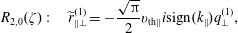 $$\begin{eqnarray}R_{2,0}(\unicode[STIX]{x1D701}):\quad \widetilde{r}_{\Vert \bot }^{(1)}=-\frac{\sqrt{\unicode[STIX]{x03C0}}}{2}v_{\text{th}\Vert }i\text{sign}(k_{\Vert })q_{\bot }^{(1)},\end{eqnarray}$$
or in real space
The closure with
 $R_{2,0}(\unicode[STIX]{x1D701})$
is naturally more precise that the closure with
$R_{2,0}(\unicode[STIX]{x1D701})$
is naturally more precise that the closure with
 $R_{1}(\unicode[STIX]{x1D701})$
, and both
$R_{1}(\unicode[STIX]{x1D701})$
, and both
 $q_{\bot }^{(1)}$
and
$q_{\bot }^{(1)}$
and
 $\widetilde{r}_{\Vert \bot }^{(1)}$
at least converge to zero for
$\widetilde{r}_{\Vert \bot }^{(1)}$
at least converge to zero for
 $\unicode[STIX]{x1D701}\gg 1$
. The closure is equivalent to (35) of Snyder et al. (Reference Snyder, Hammett and Dorland1997).
$\unicode[STIX]{x1D701}\gg 1$
. The closure is equivalent to (35) of Snyder et al. (Reference Snyder, Hammett and Dorland1997).
There are 3 another closures that can be constructed with
 $R_{2,0}(\unicode[STIX]{x1D701})$
, all of them time dependent. The first one is obtained by searching for
$R_{2,0}(\unicode[STIX]{x1D701})$
, all of them time dependent. The first one is obtained by searching for
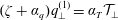 $(\unicode[STIX]{x1D701}+\unicode[STIX]{x1D6FC}_{q})q_{\bot }^{(1)}=\unicode[STIX]{x1D6FC}_{T}{\mathcal{T}}_{\bot }$
, and the solution is
$(\unicode[STIX]{x1D701}+\unicode[STIX]{x1D6FC}_{q})q_{\bot }^{(1)}=\unicode[STIX]{x1D6FC}_{T}{\mathcal{T}}_{\bot }$
, and the solution is
 $$\begin{eqnarray}\displaystyle R_{2,0}(\unicode[STIX]{x1D701}):\quad \left[\unicode[STIX]{x1D701}+\frac{i\sqrt{\unicode[STIX]{x03C0}}}{2}\right]q_{\bot }^{(1)} & = & \displaystyle \frac{p_{\bot }^{(0)}}{2}v_{\text{th}\Vert }\text{sign}(k_{\Vert }){\mathcal{T}}_{\bot };\nonumber\\ \displaystyle \left[-i\unicode[STIX]{x1D714}+\frac{\sqrt{\unicode[STIX]{x03C0}}}{2}v_{\text{th}\Vert }|k_{\Vert }|\right]q_{\bot }^{(1)} & = & \displaystyle -\frac{p_{\bot }^{(0)}}{2}v_{\text{th}\Vert }^{2}ik_{\Vert }{\mathcal{T}}_{\bot },\end{eqnarray}$$
and in real space

Alternatively, considering future normalization with parallel quantities
 $$\begin{eqnarray}R_{2,0}(\unicode[STIX]{x1D701}):\quad \left[\frac{\text{d}}{\text{d}t}-\frac{\sqrt{\unicode[STIX]{x03C0}}}{2}v_{\text{th}\Vert }\unicode[STIX]{x2202}_{z}{\mathcal{H}}\right]\frac{q_{\bot }^{(1)}}{p_{\Vert }^{(0)}}=-\frac{v_{\text{th}\Vert }^{2}}{2}\unicode[STIX]{x2202}_{z}\left[\frac{T_{\bot }^{(1)}}{T_{\Vert }^{(0)}}+a_{p}\left(a_{p}-1\right)\frac{B_{z}}{B_{0}}\right].\end{eqnarray}$$
The closures (4.118) and (4.116) are related. In the companion paper (Part 1), we derived a ‘fluid’ nonlinear equation for the perpendicular heat flux
 $\unicode[STIX]{x2202}q_{\bot }/\unicode[STIX]{x2202}t$
. Linearizing this equation yields
$\unicode[STIX]{x2202}q_{\bot }/\unicode[STIX]{x2202}t$
. Linearizing this equation yields
 $$\begin{eqnarray}\frac{\unicode[STIX]{x2202}q_{\bot }^{(1)}}{\unicode[STIX]{x2202}t}+\unicode[STIX]{x2202}_{z}\widetilde{r}_{\Vert \bot }^{(1)}+\frac{n_{0}}{2}v_{\text{th}\Vert }^{2}\unicode[STIX]{x2202}_{z}T_{\bot }^{(1)}+\frac{p_{\bot }^{(0)}}{2}v_{\text{th}\Vert }^{2}(a_{p}-1)\unicode[STIX]{x2202}_{z}\frac{B_{z}}{B_{0}}=0,\end{eqnarray}$$
where since at the linear level
 $\unicode[STIX]{x2202}_{z}\hat{b}_{z}\overset{\text{lin}}{=}0$
, the quantity
$\unicode[STIX]{x2202}_{z}\hat{b}_{z}\overset{\text{lin}}{=}0$
, the quantity
 $\unicode[STIX]{x1D735}\boldsymbol{\cdot }\hat{\boldsymbol{b}}\overset{\text{lin}}{=}(1/B_{0})(\unicode[STIX]{x2202}_{x}B_{x}+\unicode[STIX]{x2202}_{y}B_{y})=-(1/B_{0})\unicode[STIX]{x2202}_{z}B_{z}$
. Now, plugging the quasi-static closure (4.116) into the linearized heat flux equation (4.120), immediately recovers the time-dependent closure (4.118). As discussed before, the difference between
$\unicode[STIX]{x1D735}\boldsymbol{\cdot }\hat{\boldsymbol{b}}\overset{\text{lin}}{=}(1/B_{0})(\unicode[STIX]{x2202}_{x}B_{x}+\unicode[STIX]{x2202}_{y}B_{y})=-(1/B_{0})\unicode[STIX]{x2202}_{z}B_{z}$
. Now, plugging the quasi-static closure (4.116) into the linearized heat flux equation (4.120), immediately recovers the time-dependent closure (4.118). As discussed before, the difference between
 $B_{z}$
and
$B_{z}$
and
 $|\boldsymbol{B}|$
again arises only from how ‘deeply’ the linearization is done. For example, exact calculation of
$|\boldsymbol{B}|$
again arises only from how ‘deeply’ the linearization is done. For example, exact calculation of
 $\unicode[STIX]{x1D735}\boldsymbol{\cdot }\hat{\boldsymbol{b}}$
yields
$\unicode[STIX]{x1D735}\boldsymbol{\cdot }\hat{\boldsymbol{b}}$
yields
 $$\begin{eqnarray}\unicode[STIX]{x1D735}\boldsymbol{\cdot }\hat{\boldsymbol{b}}=\unicode[STIX]{x1D735}\boldsymbol{\cdot }\left(\frac{\boldsymbol{B}}{|\boldsymbol{B}|}\right)=\frac{1}{|\boldsymbol{B}|}\underbrace{\unicode[STIX]{x1D735}\boldsymbol{\cdot }\boldsymbol{B}}_{=0}+\boldsymbol{B}\boldsymbol{\cdot }\unicode[STIX]{x1D735}\left(\frac{1}{|\boldsymbol{B}|}\right)=-\frac{\hat{\boldsymbol{b}}}{|\boldsymbol{B}|}\boldsymbol{\cdot }\unicode[STIX]{x1D735}|\boldsymbol{B}|,\end{eqnarray}$$
and instead of linearizing completely, it is possible to stop the linearization at the level
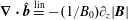 $\unicode[STIX]{x1D735}\boldsymbol{\cdot }\hat{\boldsymbol{b}}\overset{\text{lin}}{=}-(1/B_{0})\unicode[STIX]{x2202}_{z}|\boldsymbol{B}|$
.
$\unicode[STIX]{x1D735}\boldsymbol{\cdot }\hat{\boldsymbol{b}}\overset{\text{lin}}{=}-(1/B_{0})\unicode[STIX]{x2202}_{z}|\boldsymbol{B}|$
.
Another closure can be constructed by searching for
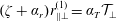 $(\unicode[STIX]{x1D701}+\unicode[STIX]{x1D6FC}_{r})r_{\Vert \bot }^{(1)}=\unicode[STIX]{x1D6FC}_{T}{\mathcal{T}}_{\bot }$
, and the solution is
$(\unicode[STIX]{x1D701}+\unicode[STIX]{x1D6FC}_{r})r_{\Vert \bot }^{(1)}=\unicode[STIX]{x1D6FC}_{T}{\mathcal{T}}_{\bot }$
, and the solution is
 $$\begin{eqnarray}\displaystyle R_{2,0}(\unicode[STIX]{x1D701}):\quad \left[\unicode[STIX]{x1D701}+\frac{i\sqrt{\unicode[STIX]{x03C0}}}{2}\right]r_{\Vert \bot }^{(1)} & = & \displaystyle -\frac{i\sqrt{\unicode[STIX]{x03C0}}}{4}p_{\bot }^{(0)}v_{\text{th}\Vert }^{2}{\mathcal{T}}_{\bot };\end{eqnarray}$$
 $$\begin{eqnarray}\displaystyle \left[-i\unicode[STIX]{x1D714}+\frac{\sqrt{\unicode[STIX]{x03C0}}}{2}v_{\text{th}\Vert }|k_{\Vert }|\right]r_{\Vert \bot }^{(1)} & = & \displaystyle -\frac{\sqrt{\unicode[STIX]{x03C0}}}{4}p_{\bot }^{(0)}v_{\text{th}\Vert }^{3}|k_{\Vert }|{\mathcal{T}}_{\bot };\nonumber\\ \displaystyle \left[\frac{\text{d}}{\text{d}t}-\frac{\sqrt{\unicode[STIX]{x03C0}}}{2}v_{\text{th}\Vert }\unicode[STIX]{x2202}_{z}{\mathcal{H}}\right]r_{\Vert \bot }^{(1)} & = & \displaystyle +\frac{\sqrt{\unicode[STIX]{x03C0}}}{4}p_{\bot }^{(0)}v_{\text{th}\Vert }^{3}\unicode[STIX]{x2202}_{z}{\mathcal{H}}\left[\frac{T_{\bot }^{(1)}}{T_{\bot }^{(0)}}+\left(\frac{T_{\bot }^{(0)}}{T_{\Vert }^{(0)}}-1\right)\frac{B_{z}}{B_{0}}\right],\nonumber\\ \displaystyle & & \displaystyle\end{eqnarray}$$
and yet another related one by searching for
 $\unicode[STIX]{x1D701}r_{\Vert \bot }^{(1)}=\unicode[STIX]{x1D6FC}_{q}q_{\bot }^{(1)}+\unicode[STIX]{x1D6FC}_{T}{\mathcal{T}}_{\bot }$
, with solution
$\unicode[STIX]{x1D701}r_{\Vert \bot }^{(1)}=\unicode[STIX]{x1D6FC}_{q}q_{\bot }^{(1)}+\unicode[STIX]{x1D6FC}_{T}{\mathcal{T}}_{\bot }$
, with solution
 $$\begin{eqnarray}\displaystyle R_{2,0}(\unicode[STIX]{x1D701}):\quad \unicode[STIX]{x1D701}r_{\Vert \bot }^{(1)} & = & \displaystyle -\frac{\unicode[STIX]{x03C0}}{4}v_{\text{th}\Vert }\text{sign}(k_{\Vert })q_{\bot }^{(1)}-\frac{i\sqrt{\unicode[STIX]{x03C0}}}{4}p_{\bot }^{(0)}v_{\text{th}\Vert }^{2}{\mathcal{T}}_{\bot };\end{eqnarray}$$
 $$\begin{eqnarray}\displaystyle -i\unicode[STIX]{x1D714}r_{\Vert \bot }^{(1)} & = & \displaystyle +\frac{\unicode[STIX]{x03C0}}{4}v_{\text{th}\Vert }^{2}ik_{\Vert }q_{\bot }^{(1)}-\frac{\sqrt{\unicode[STIX]{x03C0}}}{4}p_{\bot }^{(0)}v_{\text{th}\Vert }^{3}|k_{\Vert }|{\mathcal{T}}_{\bot };\nonumber\\ \displaystyle \frac{\text{d}}{\text{d}t}r_{\Vert \bot }^{(1)} & = & \displaystyle +\frac{\unicode[STIX]{x03C0}}{4}v_{\text{th}\Vert }^{2}\unicode[STIX]{x2202}_{z}q_{\bot }^{(1)}+\frac{\sqrt{\unicode[STIX]{x03C0}}}{4}p_{\bot }^{(0)}v_{\text{th}\Vert }^{3}\unicode[STIX]{x2202}_{z}{\mathcal{H}}\left[\frac{T_{\bot }^{(1)}}{T_{\bot }^{(0)}}+\left(\frac{T_{\bot }^{(0)}}{T_{\Vert }^{(0)}}-1\right)\frac{B_{z}}{B_{0}}\right].\nonumber\\ \displaystyle & & \displaystyle\end{eqnarray}$$
The last closure (4.125) can also be directly obtained from (4.123) by using the quasi-static closure (4.116) and
 ${\mathcal{H}}{\mathcal{H}}=-1$
. Both closures (4.125), (4.123) are not very interesting, since the quasi-static closure (4.116) for
${\mathcal{H}}{\mathcal{H}}=-1$
. Both closures (4.125), (4.123) are not very interesting, since the quasi-static closure (4.116) for
 $r_{\Vert \bot }^{(1)}$
and the time-dependent closure (4.118) for the heat flux
$r_{\Vert \bot }^{(1)}$
and the time-dependent closure (4.118) for the heat flux
 $q_{\bot }^{(1)}$
are of the same precision and much simpler to implement. Importantly, after checking the dispersion relations, closure (4.125) has to be disregarded since it can produce positive growth rate.
$q_{\bot }^{(1)}$
are of the same precision and much simpler to implement. Importantly, after checking the dispersion relations, closure (4.125) has to be disregarded since it can produce positive growth rate.
For completeness, there is also 1 time-dependent closure with
 $R_{2,1}$
approximant
$R_{2,1}$
approximant
 $\unicode[STIX]{x1D701}q_{\bot }^{(1)}=\unicode[STIX]{x1D6FC}_{T}{\mathcal{T}}_{\bot }$
that is not considered and is disregarded, since that approximant is not well behaved.
$\unicode[STIX]{x1D701}q_{\bot }^{(1)}=\unicode[STIX]{x1D6FC}_{T}{\mathcal{T}}_{\bot }$
that is not considered and is disregarded, since that approximant is not well behaved.
4.4.4 Three-pole closures
As in the 1-D case, we can suppress writing the proportionality constants (including the minus signs) and concentrate only on expressions inside of the big brackets. Continuing with the
 $R_{3,1}(\unicode[STIX]{x1D701})$
approximant
$R_{3,1}(\unicode[STIX]{x1D701})$
approximant
 $$\begin{eqnarray}\displaystyle R_{3,1}(\unicode[STIX]{x1D701}):\quad D & = & \displaystyle \left(1-\frac{4i}{\sqrt{\unicode[STIX]{x03C0}}}\unicode[STIX]{x1D701}-2\unicode[STIX]{x1D701}^{2}+2i\frac{(4-\unicode[STIX]{x03C0})}{\sqrt{\unicode[STIX]{x03C0}}}\unicode[STIX]{x1D701}^{3}\right);\end{eqnarray}$$
 $$\begin{eqnarray}\displaystyle {\mathcal{T}}_{\bot } & {\sim} & \displaystyle \frac{1}{D}\left[2i\frac{(4-\unicode[STIX]{x03C0})}{\sqrt{\unicode[STIX]{x03C0}}}\unicode[STIX]{x1D701}^{3}-2\unicode[STIX]{x1D701}^{2}-i\sqrt{\unicode[STIX]{x03C0}}\unicode[STIX]{x1D701}\right];\end{eqnarray}$$
 $$\begin{eqnarray}\displaystyle q_{\bot }^{(1)} & {\sim} & \displaystyle \frac{1}{D}\left[-i\frac{(4-\unicode[STIX]{x03C0})}{\sqrt{\unicode[STIX]{x03C0}}}\unicode[STIX]{x1D701}^{2}+\unicode[STIX]{x1D701}\right];\end{eqnarray}$$
 $$\begin{eqnarray}\displaystyle \widetilde{r}_{\Vert \bot }^{(1)} & {\sim} & \displaystyle \frac{1}{D}\left[-i\sqrt{\unicode[STIX]{x03C0}}\unicode[STIX]{x1D701}\right].\end{eqnarray}$$
No quasi-static closures are possible. A time-dependent closure can be constructed by searching for
 $(\unicode[STIX]{x1D701}+\unicode[STIX]{x1D6FC}_{r})\widetilde{r}_{\Vert \bot }^{(1)}=\unicode[STIX]{x1D6FC}_{q}q_{\bot }^{(1)}$
, and the solution reads
$(\unicode[STIX]{x1D701}+\unicode[STIX]{x1D6FC}_{r})\widetilde{r}_{\Vert \bot }^{(1)}=\unicode[STIX]{x1D6FC}_{q}q_{\bot }^{(1)}$
, and the solution reads
 $$\begin{eqnarray}\displaystyle R_{3,1}(\unicode[STIX]{x1D701}):\quad \left[\unicode[STIX]{x1D701}+\frac{i\sqrt{\unicode[STIX]{x03C0}}}{4-\unicode[STIX]{x03C0}}\right]\widetilde{r}_{\Vert \bot }^{(1)} & = & \displaystyle v_{\text{th}\Vert }\frac{\unicode[STIX]{x03C0}}{2(4-\unicode[STIX]{x03C0})}\text{sign}(k_{\Vert })q_{\bot }^{(1)};\nonumber\\ \displaystyle \left[-i\unicode[STIX]{x1D714}+\frac{\sqrt{\unicode[STIX]{x03C0}}}{4-\unicode[STIX]{x03C0}}v_{\text{th}\Vert }|k_{\Vert }|\right]\widetilde{r}_{\Vert \bot }^{(1)} & = & \displaystyle -v_{\text{th}\Vert }^{2}\frac{\unicode[STIX]{x03C0}}{2(4-\unicode[STIX]{x03C0})}ik_{\Vert }q_{\bot }^{(1)},\end{eqnarray}$$
and in real space
Continuing with the
 $R_{3,2}(\unicode[STIX]{x1D701})$
approximant
$R_{3,2}(\unicode[STIX]{x1D701})$
approximant
 $$\begin{eqnarray}\displaystyle R_{3,2}(\unicode[STIX]{x1D701}):\quad D & = & \displaystyle \left(1-\frac{3}{2}i\sqrt{\unicode[STIX]{x03C0}}\unicode[STIX]{x1D701}-2\unicode[STIX]{x1D701}^{2}+i\sqrt{\unicode[STIX]{x03C0}}\unicode[STIX]{x1D701}^{3}\right);\end{eqnarray}$$
 $$\begin{eqnarray}\displaystyle {\mathcal{T}}_{\bot } & {\sim} & \displaystyle \frac{1}{D}\left[i\sqrt{\unicode[STIX]{x03C0}}\unicode[STIX]{x1D701}^{3}-2\unicode[STIX]{x1D701}^{2}-i\sqrt{\unicode[STIX]{x03C0}}\unicode[STIX]{x1D701}\right];\end{eqnarray}$$
 $$\begin{eqnarray}\displaystyle q_{\bot }^{(1)} & {\sim} & \displaystyle \frac{1}{D}\left[-\frac{i}{2}\sqrt{\unicode[STIX]{x03C0}}\unicode[STIX]{x1D701}^{2}+\unicode[STIX]{x1D701}\right];\end{eqnarray}$$
 $$\begin{eqnarray}\displaystyle \widetilde{r}_{\Vert \bot }^{(1)} & {\sim} & \displaystyle \frac{1}{D}\left[-i\sqrt{\unicode[STIX]{x03C0}}\unicode[STIX]{x1D701}\right].\end{eqnarray}$$
Searching for
 $(\unicode[STIX]{x1D701}+\unicode[STIX]{x1D6FC}_{r})\widetilde{r}_{\Vert \bot }^{(1)}=\unicode[STIX]{x1D6FC}_{q}q_{\bot }^{(1)}$
, yields a closure
$(\unicode[STIX]{x1D701}+\unicode[STIX]{x1D6FC}_{r})\widetilde{r}_{\Vert \bot }^{(1)}=\unicode[STIX]{x1D6FC}_{q}q_{\bot }^{(1)}$
, yields a closure
 $$\begin{eqnarray}\displaystyle R_{3,2}(\unicode[STIX]{x1D701}):\quad \left[\unicode[STIX]{x1D701}+\frac{2i}{\sqrt{\unicode[STIX]{x03C0}}}\right]\widetilde{r}_{\Vert \bot }^{(1)} & = & \displaystyle v_{\text{th}\Vert }\text{sign}(k_{\Vert })q_{\bot }^{(1)};\nonumber\\ \displaystyle \left[-i\unicode[STIX]{x1D714}+\frac{2}{\sqrt{\unicode[STIX]{x03C0}}}v_{\text{th}\Vert }|k_{\Vert }|\right]\widetilde{r}_{\Vert \bot }^{(1)} & = & \displaystyle -v_{\text{th}\Vert }^{2}ik_{\Vert }q_{\bot }^{(1)},\end{eqnarray}$$
and in real space
Closures (4.131), (4.137) are equivalent to the closures of Passot & Sulem (Reference Passot and Sulem2007), after one prescribes the gyrotropic limit in that paper (and replaces the wrong coefficient in the
 $R_{3,1}(\unicode[STIX]{x1D701})$
closure introduced by Hedrick & Leboeuf (Reference Hedrick and Leboeuf1992)).
$R_{3,1}(\unicode[STIX]{x1D701})$
closure introduced by Hedrick & Leboeuf (Reference Hedrick and Leboeuf1992)).
Finally, it is indeed possible to construct an
 $o(\unicode[STIX]{x1D701}^{3})$
closure for the perpendicular quantities considered, by using the
$o(\unicode[STIX]{x1D701}^{3})$
closure for the perpendicular quantities considered, by using the
 $R_{3,0}(\unicode[STIX]{x1D701})$
approximant. The moments calculate as
$R_{3,0}(\unicode[STIX]{x1D701})$
approximant. The moments calculate as
 $$\begin{eqnarray}\displaystyle R_{3,0}(\unicode[STIX]{x1D701}):\quad D & = & \displaystyle \left(1-i\frac{\sqrt{\unicode[STIX]{x03C0}}}{4-\unicode[STIX]{x03C0}}\unicode[STIX]{x1D701}-\frac{3\unicode[STIX]{x03C0}-8}{4-\unicode[STIX]{x03C0}}\unicode[STIX]{x1D701}^{2}+2i\sqrt{\unicode[STIX]{x03C0}}\frac{\unicode[STIX]{x03C0}-3}{4-\unicode[STIX]{x03C0}}\unicode[STIX]{x1D701}^{3}\right);\end{eqnarray}$$
 $$\begin{eqnarray}\displaystyle {\mathcal{T}}_{\bot } & {\sim} & \displaystyle \frac{1}{D}\left[2i\sqrt{\unicode[STIX]{x03C0}}\frac{\unicode[STIX]{x03C0}-3}{4-\unicode[STIX]{x03C0}}\unicode[STIX]{x1D701}^{3}-\frac{3\unicode[STIX]{x03C0}-8}{4-\unicode[STIX]{x03C0}}\unicode[STIX]{x1D701}^{2}-i\sqrt{\unicode[STIX]{x03C0}}\unicode[STIX]{x1D701}\right];\end{eqnarray}$$
 $$\begin{eqnarray}\displaystyle q_{\bot }^{(1)} & {\sim} & \displaystyle \frac{1}{D}\left[-i\sqrt{\unicode[STIX]{x03C0}}\frac{\unicode[STIX]{x03C0}-3}{4-\unicode[STIX]{x03C0}}\unicode[STIX]{x1D701}^{2}+\unicode[STIX]{x1D701}\right];\end{eqnarray}$$
 $$\begin{eqnarray}\displaystyle \widetilde{r}_{\Vert \bot }^{(1)} & {\sim} & \displaystyle \frac{1}{D}\left[\frac{16-5\unicode[STIX]{x03C0}}{4-\unicode[STIX]{x03C0}}\unicode[STIX]{x1D701}^{2}-i\sqrt{\unicode[STIX]{x03C0}}\unicode[STIX]{x1D701}\right],\end{eqnarray}$$
and by searching for
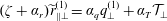 $(\unicode[STIX]{x1D701}+\unicode[STIX]{x1D6FC}_{r})\widetilde{r}_{\Vert \bot }^{(1)}=\unicode[STIX]{x1D6FC}_{q}q_{\bot }^{(1)}+\unicode[STIX]{x1D6FC}_{T}{\mathcal{T}}_{\bot }$
yields a closure
$(\unicode[STIX]{x1D701}+\unicode[STIX]{x1D6FC}_{r})\widetilde{r}_{\Vert \bot }^{(1)}=\unicode[STIX]{x1D6FC}_{q}q_{\bot }^{(1)}+\unicode[STIX]{x1D6FC}_{T}{\mathcal{T}}_{\bot }$
yields a closure
 $$\begin{eqnarray}\displaystyle R_{3,0}(\unicode[STIX]{x1D701}):\quad \left[\unicode[STIX]{x1D701}+\frac{i}{2\sqrt{\unicode[STIX]{x03C0}}}\frac{(3\unicode[STIX]{x03C0}-8)}{(\unicode[STIX]{x03C0}-3)}\right]\widetilde{r}_{\Vert \bot }^{(1)} & = & \displaystyle v_{\text{th}\Vert }\frac{4-\unicode[STIX]{x03C0}}{2(\unicode[STIX]{x03C0}-3)}\text{sign}(k_{\Vert })q_{\bot }^{(1)}\nonumber\\ \displaystyle & & \displaystyle +\,p_{\bot }^{(0)}v_{\text{th}\Vert }^{2}\frac{i}{4\sqrt{\unicode[STIX]{x03C0}}}\frac{(16-5\unicode[STIX]{x03C0})}{(\unicode[STIX]{x03C0}-3)}{\mathcal{T}}_{\bot };\nonumber\\ \displaystyle \left[-i\unicode[STIX]{x1D714}+\frac{(3\unicode[STIX]{x03C0}-8)}{2\sqrt{\unicode[STIX]{x03C0}}(\unicode[STIX]{x03C0}-3)}v_{\text{th}\Vert }|k_{\Vert }|\right]\widetilde{r}_{\Vert \bot }^{(1)} & = & \displaystyle -v_{\text{th}\Vert }^{2}\frac{4-\unicode[STIX]{x03C0}}{2(\unicode[STIX]{x03C0}-3)}ik_{\Vert }q_{\bot }^{(1)}\nonumber\\ \displaystyle & & \displaystyle +\,p_{\bot }^{(0)}v_{\text{th}\Vert }^{3}\frac{(16-5\unicode[STIX]{x03C0})}{4\sqrt{\unicode[STIX]{x03C0}}(\unicode[STIX]{x03C0}-3)}|k_{\Vert }|{\mathcal{T}}_{\bot },\end{eqnarray}$$
and the full expression in real space reads (Hunana et al. Reference Hunana, Zank, Laurenza, Tenerani, Webb, Goldstein, Velli and Adhikari2018)
 $$\begin{eqnarray}\displaystyle & & \displaystyle R_{3,0}(\unicode[STIX]{x1D701}):\quad \left[\frac{\text{d}}{\text{d}t}-\frac{(3\unicode[STIX]{x03C0}-8)}{2\sqrt{\unicode[STIX]{x03C0}}(\unicode[STIX]{x03C0}-3)}v_{\text{th}\Vert }\unicode[STIX]{x2202}_{z}{\mathcal{H}}\right]\widetilde{r}_{\Vert \bot }^{(1)}=-v_{\text{th}\Vert }^{2}\frac{4-\unicode[STIX]{x03C0}}{2(\unicode[STIX]{x03C0}-3)}\unicode[STIX]{x2202}_{z}q_{\bot }^{(1)}\nonumber\\ \displaystyle & & \displaystyle -\,p_{\bot }^{(0)}v_{\text{th}\Vert }^{3}\frac{(16-5\unicode[STIX]{x03C0})}{4\sqrt{\unicode[STIX]{x03C0}}(\unicode[STIX]{x03C0}-3)}\unicode[STIX]{x2202}_{z}{\mathcal{H}}\left[\frac{T_{\bot }^{(1)}}{T_{\bot }^{(0)}}+\left(\frac{T_{\bot }^{(0)}}{T_{\Vert }^{(0)}}-1\right)\frac{B_{z}}{B_{0}}\right],\end{eqnarray}$$
or again considering normalization with respect to parallel quantities
 $$\begin{eqnarray}\displaystyle & & \displaystyle R_{3,0}(\unicode[STIX]{x1D701}):\quad \left[\frac{\text{d}}{\text{d}t}-\frac{(3\unicode[STIX]{x03C0}-8)}{2\sqrt{\unicode[STIX]{x03C0}}(\unicode[STIX]{x03C0}-3)}v_{\text{th}\Vert }\unicode[STIX]{x2202}_{z}{\mathcal{H}}\right]\frac{\widetilde{r}_{\Vert \bot }^{(1)}}{p_{\Vert }^{(0)}}=-v_{\text{th}\Vert }^{2}\frac{4-\unicode[STIX]{x03C0}}{2(\unicode[STIX]{x03C0}-3)}\unicode[STIX]{x2202}_{z}\frac{q_{\bot }^{(1)}}{p_{\Vert }^{(0)}}\nonumber\\ \displaystyle & & \displaystyle \qquad -\,v_{\text{th}\Vert }^{3}\frac{(16-5\unicode[STIX]{x03C0})}{4\sqrt{\unicode[STIX]{x03C0}}(\unicode[STIX]{x03C0}-3)}\unicode[STIX]{x2202}_{z}{\mathcal{H}}\left[\frac{T_{\bot }^{(1)}}{T_{\Vert }^{(0)}}+a_{p}\left(a_{p}-1\right)\frac{B_{z}}{B_{0}}\right].\end{eqnarray}$$
The
 $R_{3,0}(\unicode[STIX]{x1D701})$
has precision
$R_{3,0}(\unicode[STIX]{x1D701})$
has precision
 $o(\unicode[STIX]{x1D701}^{3})$
,
$o(\unicode[STIX]{x1D701}^{3})$
,
 $o(1/\unicode[STIX]{x1D701}^{2})$
.
$o(1/\unicode[STIX]{x1D701}^{2})$
.
4.5 Table of moments
$(T_{\bot },q_{\bot },\widetilde{r}_{\Vert \bot })$
for various Padé approximants

The following summarizing table for quantities
 ${\mathcal{T}}_{\bot }(T_{\bot }^{(1)}),q_{\bot }^{(1)},\widetilde{r}_{\Vert \bot }^{(1)}$
is created to clearly see the possibilities of a closure. All the proportionality constants (including the minus signs) and including the common denominator of
${\mathcal{T}}_{\bot }(T_{\bot }^{(1)}),q_{\bot }^{(1)},\widetilde{r}_{\Vert \bot }^{(1)}$
is created to clearly see the possibilities of a closure. All the proportionality constants (including the minus signs) and including the common denominator of
 $R(\unicode[STIX]{x1D701})$
, are suppressed here. The approximants
$R(\unicode[STIX]{x1D701})$
, are suppressed here. The approximants
 $R_{2,1},R_{4,5},R_{6,9},R_{8,13}$
are marked with an asterisk ‘*’, because these do not account for the Landau residue and are not well behaved. These approximants are provided only for completeness and should be disregarded.
$R_{2,1},R_{4,5},R_{6,9},R_{8,13}$
are marked with an asterisk ‘*’, because these do not account for the Landau residue and are not well behaved. These approximants are provided only for completeness and should be disregarded.

By observing the table, there are altogether 2 possible quasi-static closures,
 $$\begin{eqnarray}\displaystyle R_{1}:\quad q_{\bot }^{(1)}=\unicode[STIX]{x1D6FC}_{T}{\mathcal{T}}_{\bot }; & & \displaystyle \nonumber\\ \displaystyle R_{2,0}:\quad \widetilde{r}_{\Vert \bot }^{(1)}=\unicode[STIX]{x1D6FC}_{q}q_{\bot }^{(1)}, & & \displaystyle\end{eqnarray}$$
and 6 time-dependent closures,
 $$\begin{eqnarray}\displaystyle R_{2,0}:\quad (\unicode[STIX]{x1D701}+\unicode[STIX]{x1D6FC}_{q})q_{\bot }^{(1)} & = & \displaystyle \unicode[STIX]{x1D6FC}_{T}{\mathcal{T}}_{\bot };\quad (\unicode[STIX]{x1D701}+\unicode[STIX]{x1D6FC}_{r})\widetilde{r}_{\Vert \bot }^{(1)}=\unicode[STIX]{x1D6FC}_{T}{\mathcal{T}}_{\bot };\quad \cancel{\unicode[STIX]{x1D701}\widetilde{r}_{\Vert \bot }^{(1)}=\unicode[STIX]{x1D6FC}_{q}q_{\bot }^{(1)}+\unicode[STIX]{x1D6FC}_{T}{\mathcal{T}}_{\bot }};\nonumber\\ \displaystyle R_{3,0}:\quad (\unicode[STIX]{x1D701}+\unicode[STIX]{x1D6FC}_{r})\widetilde{r}_{\Vert \bot }^{(1)} & = & \displaystyle \unicode[STIX]{x1D6FC}_{q}q_{\bot }^{(1)}+\unicode[STIX]{x1D6FC}_{T}{\mathcal{T}}_{\bot };\nonumber\\ \displaystyle R_{3,1}:\quad (\unicode[STIX]{x1D701}+\unicode[STIX]{x1D6FC}_{r})\widetilde{r}_{\Vert \bot }^{(1)} & = & \displaystyle \unicode[STIX]{x1D6FC}_{q}q_{\bot }^{(1)};\nonumber\\ \displaystyle R_{3,2}:\quad (\unicode[STIX]{x1D701}+\unicode[STIX]{x1D6FC}_{r})\widetilde{r}_{\Vert \bot }^{(1)} & = & \displaystyle \unicode[STIX]{x1D6FC}_{q}q_{\bot }^{(1)}.\end{eqnarray}$$
We briefly checked the dispersion relations that these closures yield for parallel propagation (proton species only, electrons cold), where the
 $q_{\bot }^{(1)}$
and
$q_{\bot }^{(1)}$
and
 $\widetilde{r}_{\Vert \bot }^{(1)}$
closures produce only higher-order modes. This eliminated one
$\widetilde{r}_{\Vert \bot }^{(1)}$
closures produce only higher-order modes. This eliminated one
 $R_{2,0}$
closure that produced a growing mode. The
$R_{2,0}$
closure that produced a growing mode. The
 $R_{1}$
closure yields
$R_{1}$
closure yields
 $\unicode[STIX]{x1D701}=-i/\sqrt{\unicode[STIX]{x03C0}}$
; the remaining
$\unicode[STIX]{x1D701}=-i/\sqrt{\unicode[STIX]{x03C0}}$
; the remaining
 $R_{2,0}$
closures yield
$R_{2,0}$
closures yield
 $\unicode[STIX]{x1D701}=\pm \sqrt{8-\unicode[STIX]{x03C0}}/4-i\sqrt{\unicode[STIX]{x03C0}}/4$
(result reported also in the Appendix of Hunana et al. (Reference Hunana, Laveder, Passot, Sulem and Borgogno2011)), the
$\unicode[STIX]{x1D701}=\pm \sqrt{8-\unicode[STIX]{x03C0}}/4-i\sqrt{\unicode[STIX]{x03C0}}/4$
(result reported also in the Appendix of Hunana et al. (Reference Hunana, Laveder, Passot, Sulem and Borgogno2011)), the
 $R_{3,0}$
closure yields
$R_{3,0}$
closure yields
 $\unicode[STIX]{x1D701}=\pm 0.92-0.91i;\unicode[STIX]{x1D701}=-1.02i$
; the
$\unicode[STIX]{x1D701}=\pm 0.92-0.91i;\unicode[STIX]{x1D701}=-1.02i$
; the
 $R_{3,1}$
closure yields
$R_{3,1}$
closure yields
 $\unicode[STIX]{x1D701}=\pm 0.96-0.64i;\unicode[STIX]{x1D701}=-0.78i$
; and the
$\unicode[STIX]{x1D701}=\pm 0.96-0.64i;\unicode[STIX]{x1D701}=-0.78i$
; and the
 $R_{3,2}$
closure yields
$R_{3,2}$
closure yields
 $\unicode[STIX]{x1D701}=\pm 1.04-0.33i$
;
$\unicode[STIX]{x1D701}=\pm 1.04-0.33i$
;
 $\unicode[STIX]{x1D701}=-0.47i$
.
$\unicode[STIX]{x1D701}=-0.47i$
.
5 Conclusions
We offer a brief summary of the major results discussed throughout the text.
∙ The kinetic Vlasov equation implicitly contains ‘singularities’ in velocity space, referred to as wave–particle resonances. These resonances occur because particles of a given species travelling along magnetic field lines with a velocity component
$v_{\Vert }$
interact with plasma waves propagating in that system with a parallel phase speed
$(\unicode[STIX]{x1D714}+n\unicode[STIX]{x1D6FA})/k_{\Vert }$
, where
$\unicode[STIX]{x1D6FA}$
is the cyclotron frequency for that given species and
$n=0,\pm 1,\pm 2\ldots$
is an integer. Wave–particle resonances can be separated into Landau resonances (
$n=0$
) and cyclotron resonances (
$n\neq 0$
).∙ The presence of wave–particle resonances in the Vlasov equation is revealed by considering perturbations
$f^{(1)}=f-f_{0}$
around an equilibrium distribution function
$f_{0}$
, and by obtaining an explicit expression for
$f^{(1)}$
that satisfies the Vlasov equation. For example, in a simplified 1-D electrostatic geometry (which can be viewed as electrostatic propagation along
$\boldsymbol{B}_{0}$
), the perturbations read
$f^{(1)}=-(iqE_{\Vert }/m)(\unicode[STIX]{x2202}f_{0}/\unicode[STIX]{x2202}v_{\Vert })/(\unicode[STIX]{x1D714}-v_{\Vert }k_{\Vert })$
, and contain Landau resonances.∙ Obtaining
$f^{(1)}$
in a general 3-D electromagnetic geometry requires quite a complicated procedure of integration along an unperturbed orbit (zero-order trajectory, from time
$t^{\prime }=-\infty$
to
$t^{\prime }=t$
), see (2.15). The procedure can be considered as a core of any plasma book and here it is summarized in appendix C. General
$f^{(1)}$
perturbations around a gyrotropic
$f_{0}$
are given by (C 47). Prescribing a bi-Maxwellian
$f_{0}$
yields (C 53), and prescribing a bi-kappa
$f_{0}$
yields (C 57). Obviously, perturbations
$f^{(1)}\sim 1/(\unicode[STIX]{x1D714}-v_{\Vert }k_{\Vert }-n\unicode[STIX]{x1D6FA})$
, and contain Landau resonances and cyclotron resonances.∙ After an
$f^{(1)}$
is obtained, integration over velocity space can be performed, eventually yielding an infinite hierarchy of ‘kinetic’ moments. Combining Maxwell’s equations
$\unicode[STIX]{x1D735}\times \boldsymbol{B}=(4\unicode[STIX]{x03C0}/c)\boldsymbol{j}+(1/c)\unicode[STIX]{x2202}\boldsymbol{E}/\unicode[STIX]{x2202}t$
and
$\unicode[STIX]{x1D735}\times \boldsymbol{E}=-(1/c)\unicode[STIX]{x2202}\boldsymbol{B}/\unicode[STIX]{x2202}t$
yields the following wave equation (5.1)Therefore, to obtain the full dispersion relation of kinetic theory, it is sufficient to stop the hierarchy at the first-order (velocity) moment, which determines the current$$\begin{eqnarray}\boldsymbol{k}\times (\boldsymbol{k}\times \boldsymbol{E})+\frac{\unicode[STIX]{x1D714}^{2}}{c^{2}}\left(\frac{4\unicode[STIX]{x03C0}i}{\unicode[STIX]{x1D714}}\boldsymbol{j}+\boldsymbol{E}\right)=0.\end{eqnarray}$$
$\boldsymbol{j}=\sum _{r}q_{r}n_{r}\boldsymbol{u}_{r}=\unicode[STIX]{x1D748}\boldsymbol{\cdot }\boldsymbol{E}$
. Calculations of pressure or higher-order kinetic moments are not necessary and are thus typically omitted (provided that the full non-gyrotropic
$f^{(1)}$
is considered, so that the perpendicular velocity moments
$\boldsymbol{u}_{\bot }$
are non-zero). In addition to the conductivity tensor
$\unicode[STIX]{x1D748}$
, one can also use the susceptibility tensor
$\unicode[STIX]{x1D74C}=(4\unicode[STIX]{x03C0}i/\unicode[STIX]{x1D714})\unicode[STIX]{x1D748}$
, and the dielectric tensor
$\unicode[STIX]{x1D750}=\unicode[STIX]{x1D74C}+\unicode[STIX]{x1D644}$
(the
$\unicode[STIX]{x1D644}$
is a unit matrix and here it represents contributions of the displacement current). The definitions of
$\unicode[STIX]{x1D74C}$
and
$\unicode[STIX]{x1D750}$
are naturally motivated by the wave equation (5.1).∙ In Landau fluid models, the kinetic hierarchy has to be calculated at least up to the third-order (heat flux) moment, or preferably, the fourth-order moment
$\boldsymbol{r}$
(or beyond). Importantly, a closure has to be found where the last retained moment is expressed through lower-order moments. Subsequently, a simplification of
$f^{(1)}$
is necessary, and in general one needs to impose a low-frequency limit
$\unicode[STIX]{x1D714}/\unicode[STIX]{x1D6FA}\ll 1$
, which eliminates the
$n\neq 0$
cyclotron resonances. The exception is the 1-D electrostatic geometry, where the low-frequency restriction is not required, and closures for arbitrary frequencies (and wavelengths) can be obtained.∙ In the 3-D electromagnetic geometry, we restricted our attention to perturbations
$f^{(1)}$
in the gyrotropic limit, see (4.14). In this geometry, in addition to the low-frequency limit, one also assumes that the gyroradius is small, which corresponds to the limit
$k_{\bot }v_{\bot }/\unicode[STIX]{x1D6FA}\ll 1$
(the gyroradius is defined as
$v_{\text{th}\bot }/\unicode[STIX]{x1D6FA}$
, but here the limit is applied directly on
$f^{(1)}$
before integration over velocity space). It is rather mind boggling that to obtain the correct
$f^{(1)}$
in the laboratory reference frame, one needs to first calculate the complicated integration around the unperturbed orbit, and only then prescribe the gyrotropic limit.∙ Alternatively, the
$f^{(1)}$
in the gyrotropic limit can be derived by using the guiding-centre reference frame, and by imposing the conservation of the magnetic moment in the Vlasov equation from the beginning. Then, it is possible to show that various terms in
$f^{(1)}$
correspond to the conservation of magnetic moment, electrostatic Coulomb force (which yields Landau damping), and magnetic mirror force (which yields transit-time damping, also called Barnes damping), see (4.15) and § 4.2.∙ We considered Landau fluid closures only for a bi-Maxwellian
$f_{0}$
(which in the 1-D geometry simplifies to a Maxwellian
$f_{0}$
), even though one should be able to construct closures for a different
$f_{0}$
with a similar technique.∙ In the 1-D electrostatic geometry, the kinetic hierarchy calculated up to the fourth-order moment is given by (3.20)–(3.26). All the moments contain the plasma response function
$R(\unicode[STIX]{x1D701})=1+\unicode[STIX]{x1D701}Z(\unicode[STIX]{x1D701})$
, where
$Z(\unicode[STIX]{x1D701})$
is the plasma dispersion function defined by (2.35), and the variable
$\unicode[STIX]{x1D701}=\unicode[STIX]{x1D714}/(|k_{\Vert }|v_{\text{th}\Vert })$
. Importantly, the
$\unicode[STIX]{x1D701}$
variable is here defined with
$|k_{\Vert }|=\text{sign}(k_{\Vert })k_{\Vert }$
. If the
$\unicode[STIX]{x1D701}$
variable is defined with
$k_{\Vert }$
, the plasma dispersion function has to be redefined to
$Z_{0}(\unicode[STIX]{x1D701})$
, equation (2.39). The
$R(\unicode[STIX]{x1D701})$
in the kinetic hierarchy can be quickly interpreted according to (2.49).∙ It is impossible to find any ‘direct’ rigorously exact fluid closure in the kinetic hierarchy of moments. In other words, it is impossible to take the last retained
$n$
th-order moment, and directly express it through lower-order moments by using exact un-approximated
$R(\unicode[STIX]{x1D701})$
function, in such a way that the closure eliminates the
$R(\unicode[STIX]{x1D701})$
function. Technically, such a closure is possible only when
$n\rightarrow \infty$
.∙ To find a closure, the
$R(\unicode[STIX]{x1D701})$
in the kinetic hierarchy needs to be analytically approximated, for example by a suitable Padé approximant
$R_{n,n^{\prime }}(\unicode[STIX]{x1D701})$
(as a ratio of two polynomials in
$\unicode[STIX]{x1D701}$
). Approximants
$R_{n,n^{\prime }}(\unicode[STIX]{x1D701})$
are constructed by matching power-series expansions
$|\unicode[STIX]{x1D701}|\ll 1$
of
$R(\unicode[STIX]{x1D701})$
, see (3.33), and asymptotic-series expansions
$|\unicode[STIX]{x1D701}|\gg 1$
, see (3.67). Perhaps the most convenient is to expand (3.193).∙ Importantly, contributions from the Landau residue
${\sim}\unicode[STIX]{x1D701}e^{-\unicode[STIX]{x1D701}^{2}}$
in
$R(\unicode[STIX]{x1D701})$
are retained in the power-series expansion, however, the contributions are eliminated in the asymptotic series expansion (since there is no asymptotic expansion of
$e^{-\unicode[STIX]{x1D701}^{2}}$
). The same procedure is used in the kinetic solver WHAMP. Consequently, deeply down in the lower complex plane where damping becomes very large, Padé approximants of
$R(\unicode[STIX]{x1D701})$
become less accurate.∙ Another example is the Langmuir mode, see § 3.15, where in the long-wavelength limit the frequency
$\unicode[STIX]{x1D714}$
does not decrease, but is equal to the plasma frequency. Thus,
$|\unicode[STIX]{x1D701}|\gg 1$
, and the Landau damping of the Langmuir mode in the long-wavelength limit typically disappears much more rapidly in kinetic theory than in Landau fluid models (see figure 7), which is a direct consequence of the missing
$\unicode[STIX]{x1D701}e^{-\unicode[STIX]{x1D701}^{2}}$
in the asymptotic expansions of
$R(\unicode[STIX]{x1D701})$
. Nevertheless, at spatial scales that are shorter than five Debye lengths, the damping of the Langmuir mode can be captured very accurately in a fluid framework, see closure (3.421) and figure 10. Notably, it was indeed the example of the Langmuir mode that was used by Landau (Reference Landau1946) to predict this collisionless damping phenomenon.∙ We introduced a new classification scheme, that we consider more natural than previous classifications. The
$n$
index in
$R_{n,n^{\prime }}(\unicode[STIX]{x1D701})$
represents the number of poles, and the ‘basic’ approximant
$R_{n,0}(\unicode[STIX]{x1D701})$
is defined as having the correct (leading-order) asymptote
$-1/(2\unicode[STIX]{x1D701}^{2})$
, see (3.104). The
$R_{n,0}(\unicode[STIX]{x1D701})$
therefore correctly captures the asymptotic profile of the zeroth-order (density) moment, and approximants with less asymptotic points should be avoided if possible. The
$R_{n,n^{\prime }}(\unicode[STIX]{x1D701})$
is defined as using
$n^{\prime }$
additional points in the asymptotic-series expansion in comparison to
$R_{n,0}(\unicode[STIX]{x1D701})$
. The exception is the one-pole approximant
$R_{1}(\unicode[STIX]{x1D701})=1/(1-i\sqrt{\unicode[STIX]{x03C0}}\unicode[STIX]{x1D701})$
, which obviously does not have the correct asymptote.∙ Approximant
$R_{n,n^{\prime }}(\unicode[STIX]{x1D701})$
has power-series precision
$o(\unicode[STIX]{x1D701}^{2n-3-n^{\prime }})$
and asymptotic-series precision
$o(\unicode[STIX]{x1D701}^{-2-n^{\prime }})$
. Analytic forms of two-pole approximants of
$R(\unicode[STIX]{x1D701})$
and
$Z(\unicode[STIX]{x1D701})$
are given in § 3.3.1, three-pole approximants in § 3.3.2 and four-pole approximants in § 3.3.3. In appendix A, we provide valuable tables of five-, six-, seven- and eight-pole approximants of
$R(\unicode[STIX]{x1D701})$
, many in an analytic form. The precision of all approximants is compared in § 3.5.∙ The limit
$|\unicode[STIX]{x1D701}|\ll 1$
can be viewed as an isothermal limit, and
$|\unicode[STIX]{x1D701}|\gg 1$
can be viewed as an adiabatic limit. Therefore, classical adiabatic fluid models discussed in Part 1 can be obtained by considering a high phase-speed limit
$|\unicode[STIX]{x1D714}/k_{\Vert }|\gg v_{\text{th}\Vert }$
. The exception is the generalized isothermal (‘static’) closure used to capture the mirror instability, where a low phase-speed limit
$|\unicode[STIX]{x1D714}/k_{\Vert }|\ll v_{\text{th}\Vert }$
must be used.∙ In many instances, solely expanding in
$|\unicode[STIX]{x1D701}|\ll 1$
or
$|\unicode[STIX]{x1D701}|\gg 1$
is not appropriate, and the
$R(\unicode[STIX]{x1D701})$
together with
$Z(\unicode[STIX]{x1D701})$
can be viewed as the most important functions of kinetic theory. For example, considering a proton–electron plasma at scales that are much longer than the Debye length, the dispersion relation of the parallel ion-acoustic mode is given by (3.366), and for equal proton and electron temperatures it reads
$R(\unicode[STIX]{x1D701}_{p})+R(\unicode[STIX]{x1D701}_{e})=0$
. No expansion of
$R(\unicode[STIX]{x1D701})$
is possible, since the numerical solution is
$\unicode[STIX]{x1D701}_{p}=\pm 1.46-0.63i$
. Only when electrons are hot and
$T_{\Vert e}^{(0)}\gg T_{\Vert p}^{(0)}$
, can a simplified dispersion relation for the ion-acoustic mode be obtained by prescribing
$|\unicode[STIX]{x1D701}_{p}|\gg 1$
and
$|\unicode[STIX]{x1D701}_{e}|\ll 1$
. By employing Padé approximants
$R_{n,n^{\prime }}(\unicode[STIX]{x1D701})$
in Landau fluid closures, the
$R(\unicode[STIX]{x1D701})$
function is analytically approximated for all
$\unicode[STIX]{x1D701}$
values, see figures 2 and 3.∙ For the 1-D electrostatic geometry, all the Landau fluid closures that can be constructed for the heat flux
$q$
and the fourth-order moment perturbation
$\widetilde{r}=r-3p^{2}/\unicode[STIX]{x1D70C}$
, are summarized in (3.241)–(3.242). The same closures are obtained in the 3-D electromagnetic geometry for parallel moments
$q_{\Vert }$
and
$\widetilde{r}_{\Vert \Vert }$
. These closures do not have any restrictions for frequencies and wavenumbers, and are therefore valid from the largest astrophysical scales down to the Debye length.∙ Landau fluid closures can be separated into two categories. (I) A closure is called static (or quasi-static), when the last retained moment
$X_{l}$
is directly expressed through lower-order moments. (II) A closure is called dynamic (or time dependent), when
$\unicode[STIX]{x1D701}X_{l}+\unicode[STIX]{x1D6FC}X_{l}$
is expressed through lower-order moments (where
$\unicode[STIX]{x1D6FC}$
is a coefficient). After a dynamic closure is transformed to real space,
$\unicode[STIX]{x2202}/\unicode[STIX]{x2202}t$
is replaced by the convective derivative
$\text{d}/\text{d}t$
to preserve Galilean invariance.∙ In real space, all the closures contain the negative Hilbert transform operator
${\mathcal{H}}$
, defined according to
${\mathcal{H}}f(z)=-(1/\unicode[STIX]{x03C0}z)\ast f(z)=-(1/\unicode[STIX]{x03C0})V.P.\int _{-\infty }^{\infty }f(z-z^{\prime })/z^{\prime }\,\text{d}z^{\prime }$
, where
$\ast$
represents convolution. The
${\mathcal{H}}$
operator in closures comes from Fourier space, where it is equal to
$i\text{sign}(k_{\Vert })$
. In real space, the
${\mathcal{H}}$
operator represents non-locality of closures, and, ideally, the integrals in
${\mathcal{H}}f(z)$
should be calculated along magnetic field lines. The effect is pronounced in numerical simulations, where calculating the Hilbert transform along the ambient magnetic field
$B_{0}$
can cause instabilities, see Passot et al. (Reference Passot, Henri, Laveder and Sulem2014).∙ For example, the simplest closure for the heat flux
$q_{\Vert }$
is given by (3.261) of Hammett & Perkins (Reference Hammett and Perkins1990) (or equivalently by (4.94) when written in the 3-D geometry). The simplest closure for the heat flux
$q_{\bot }$
is given by (4.108) of Snyder et al. (Reference Snyder, Hammett and Dorland1997). Both closures are proportional to the Hilbert transform of temperatures
$T_{\Vert }$
,
$T_{\bot }$
. Therefore, Landau fluid closures yield gyrotropic heat fluxes
$q_{\Vert }$
,
$q_{\bot }$
that are non-local, and influenced by temperatures along the entire magnetic field line. Notably, this is in contrast to ‘classical’ non-gyrotropic heat flux vectors
$\boldsymbol{S}_{\bot }^{\Vert }$
,
$\boldsymbol{S}_{\bot }^{\bot }$
discussed in Part 1, which were local and proportional to the gradient of temperatures.∙ In the 3-D electromagnetic geometry in the gyrotropic limit, the closure for the perturbation
$\widetilde{r}_{\bot \bot }$
is simply
$\widetilde{r}_{\bot \bot }=0$
. One needs to consider only closures for
$q_{\bot }$
and
$\widetilde{r}_{\Vert \bot }$
, which are given in § 4.4 and summarized in (4.145)–(4.146).∙ Only one static closure for
$q_{\bot }$
is available, the closure (4.108) of Snyder et al. (Reference Snyder, Hammett and Dorland1997). However, the closure is obtained with the
$R_{1}(\unicode[STIX]{x1D701})$
approximant. Since
$q_{\bot }\sim \unicode[STIX]{x1D701}R(\unicode[STIX]{x1D701})$
, see (4.92) or (4.105), using
$R_{1}(\unicode[STIX]{x1D701})$
implies that for large
$\unicode[STIX]{x1D701}$
values the heat flux does not disappear and instead converges to a constant value, which is erroneous. Additionally, for
$\unicode[STIX]{x1D701}>1$
the real part of
$R_{1}(\unicode[STIX]{x1D701})$
even has the wrong sign, see figure 2. The
$R_{1}(\unicode[STIX]{x1D701})$
is still a valuable approximant for small
$|\unicode[STIX]{x1D701}|\ll 1$
values, and a Landau fluid model with static heat flux closures (4.94), (4.108) recovers the correct mirror threshold.∙ If one comes to the conclusion that the
$R_{1}(\unicode[STIX]{x1D701})$
approximant is unsatisfactory, then no static closure for
$q_{\bot }$
is available. Consequently, 3-D Landau fluid simulations are possible only if the heat fluxes
$q_{\Vert }$
,
$q_{\bot }$
are described by time-dependent equations. Of course, one could possibly consider a model with a static
$q_{\Vert }$
closure and time-dependent
$q_{\bot }$
closure.∙ Perhaps, the most natural way to perform 3-D Landau fluid simulations is to keep the ‘classical’ nonlinear evolution equations for
$q_{\Vert }$
and
$q_{\bot }$
obtained in Part 1, and use static Landau fluid closures for the perturbations of the fourth-order moment. Of course, it is easy to imagine that, in some numerical simulations, the heat flux equations might be ‘too nonlinear’, i.e. responsible for instabilities. In such a case, the dynamic (linear) heat flux closures might be useful to verify the instability.∙ For the
$\widetilde{r}_{\Vert \Vert }$
moment, there are 3 static closures available: the
$R_{4,2}$
closure (3.227), the
$R_{4,3}$
closure (3.234) of Hammett & Perkins (Reference Hammett and Perkins1990) and the
$R_{4,4}$
closure (3.240). In real space, the
$R_{4,2}$
closure is given by (3.267), the
$R_{4,3}$
closure by (3.266) and the
$R_{4,4}$
closure by (3.268). The
$R_{4,2}$
closure has the highest power-series precision
$o(\unicode[STIX]{x1D701}^{3})$
, and the
$R_{4,4}$
closure has the highest asymptotic-series precision
$o(\unicode[STIX]{x1D701}^{-6})$
. It is of course difficult to recommend which closure is clearly better without considering a specific situation.∙ We considered the example of the ion-acoustic mode, see figures 5 and 6 and associated discussion. The
$R_{4,4}$
closure can be useful for simulations with sufficiently high electron temperatures, namely
$\unicode[STIX]{x1D70F}=T_{e}/T_{p}>15$
, which corresponds to
$\unicode[STIX]{x1D701}_{p}>3$
. However, such simulations will be perhaps not performed very frequently. In the most interesting regime with comparable proton and electron temperatures (or
$\unicode[STIX]{x1D70F}\in [1,5]$
) the most precise static closure is by far the
$R_{4,2}$
closure. Nevertheless, the
$R_{4,3}$
closure is still a globally precise closure. We can only recommend to use both the
$R_{4,2}$
closure (3.267) of Hunana et al. (Reference Hunana, Zank, Laurenza, Tenerani, Webb, Goldstein, Velli and Adhikari2018) and the
$R_{4,3}$
closure (3.266) of Hammett & Perkins (Reference Hammett and Perkins1990), and clarify possible differences in numerical simulations. The differences might be more pronounced during nonlinear dynamics.∙ As an example, Landau fluid simulations of turbulence typically show a curious behaviour (see e.g. Perrone et al. (Reference Perrone, Passot, Laveder, Valentini, Sulem, Zouganelis, Veltri and Servidio2018) and references therein), that at sub-proton scales, the spectrum of the parallel velocity field
$u_{\Vert }$
is much steeper in kinetic simulations than in Landau fluid simulations. In contrast to the
$R_{4,3}$
closure, our
$R_{4,2}$
closure contains the parallel velocity
$u_{\Vert }$
. It would be interesting to explore if the
$R_{4,2}$
closure influences the
$u_{\Vert }$
spectrum.∙ For the
$\widetilde{r}_{\Vert \bot }$
moment, there is only one static closure, the
$R_{2,0}$
closure (4.116) of Snyder et al. (Reference Snyder, Hammett and Dorland1997).∙ If higher precision is desired, one can use dynamic closures for the
$\widetilde{r}_{\Vert \Vert }$
and
$\widetilde{r}_{\Vert \bot }$
moments, which however introduces two additional evolution equations. Of course, it is possible to use dynamic closure only for the
$\widetilde{r}_{\Vert \bot }$
moment. As discussed above, it appears that closures with the highest power-series precision (p.s.p.) are the most desirable (at least for
$T_{e}\sim T_{p}$
). Concerning the
$\widetilde{r}_{\Vert \Vert }$
moment, the static
$R_{4,2}$
closure has p.s.p.
$o(\unicode[STIX]{x1D701}^{3})$
. Thus, it is possible to have a view that a worthy dynamic closure for
$\widetilde{r}_{\Vert \Vert }$
should have a p.s.p.
$o(\unicode[STIX]{x1D701}^{4})$
. There is only one such closure, the
$R_{5,3}$
closure (3.339) of Hunana et al. (Reference Hunana, Zank, Laurenza, Tenerani, Webb, Goldstein, Velli and Adhikari2018).∙ Concerning dynamic closures for the
$\widetilde{r}_{\Vert \bot }$
moment, the static
$R_{2,0}$
closure (4.116) has a p.s.p.
$o(\unicode[STIX]{x1D701})$
. Therefore, a worthy dynamic closure for the
$\widetilde{r}_{\Vert \bot }$
moment should have a p.s.p.
$o(\unicode[STIX]{x1D701}^{2})$
, or higher. There are only two such closures. One with a p.s.p.
$o(\unicode[STIX]{x1D701}^{2})$
, the
$R_{3,1}$
closure (4.131) of Passot & Sulem (Reference Passot and Sulem2007); and one with a p.s.p.
$o(\unicode[STIX]{x1D701}^{3})$
, the
$R_{3,0}$
closure (4.143) of Hunana et al. (Reference Hunana, Zank, Laurenza, Tenerani, Webb, Goldstein, Velli and Adhikari2018).∙ To summarize, if one desires the highest power-series precision that is available at the fourth-order moment level, one should use the dynamic
$R_{5,3}$
closure (3.339) for the
$\widetilde{r}_{\Vert \Vert }$
moment, and the dynamic
$R_{3,0}$
closure (4.143) for the
$\widetilde{r}_{\Vert \bot }$
moment. Nevertheless, the dynamic closures might not be worth the computational cost, and it is possible to have a view that the static closures are sufficiently precise. In that case, for the
$\widetilde{r}_{\Vert \Vert }$
moment one should use either the
$R_{4,2}$
closure (3.267), or the
$R_{4,3}$
closure (3.266) (see the discussion above) and for the
$\widetilde{r}_{\Vert \bot }$
moment the
$R_{2,0}$
closure (4.116). Alternatively, one can use a dynamic closure only for the
$\widetilde{r}_{\Vert \bot }$
moment. In that case, it is possible to match the power-series precision of
$\widetilde{r}_{\Vert \Vert }$
and
$\widetilde{r}_{\Vert \bot }$
moments. The precision
$o(\unicode[STIX]{x1D701}^{2})$
is achieved by using the
$R_{4,3}$
closure (3.266) for the
$\widetilde{r}_{\Vert \Vert }$
moment and the
$R_{3,1}$
closure (4.131) for the
$\widetilde{r}_{\Vert \bot }$
moment. The precision
$o(\unicode[STIX]{x1D701}^{3})$
is achieved by using the
$R_{4,2}$
closure (3.267) for the
$\widetilde{r}_{\Vert \Vert }$
moment and the
$R_{3,0}$
closure (4.143) for the
$\widetilde{r}_{\Vert \bot }$
moment.∙ The most surprising result discussed in Part 2 is the observation that some closures reproduce a considered kinetic dispersion relation exactly, after
$R(\unicode[STIX]{x1D701})$
is replaced by the approximant
$R_{n,n^{\prime }}(\unicode[STIX]{x1D701})$
used to obtain that fluid closure. We consider this observation as highly non-trivial and not obvious. For example, a 1-D fluid model described by (3.371)–(3.378) that uses the
$R_{4,3}$
closure for the
$\widetilde{r}_{\Vert \Vert }$
moment, has a dispersion relation that is equivalent to the kinetic dispersion relation (3.366), after the
$R(\unicode[STIX]{x1D701})$
is replaced by
$R_{4,3}(\unicode[STIX]{x1D701})$
. The results are equivalent only after the
$R_{4,3}(\unicode[STIX]{x1D701}_{p})$
and
$R_{4,3}(\unicode[STIX]{x1D701}_{e})$
terms in (3.366) are transferred to the common denominator and the resulting numerator is made to be equal to zero. That example concerns the ion-acoustic mode, but the same observation is true for the Langmuir mode as well, see § 3.15, dispersion relation (3.396). We called such closures ‘reliable’, or physically meaningful.∙ We only verified which closures are ‘reliable’ on dispersion relations of the ion-acoustic mode and the Langmuir mode in the 1-D electrostatic geometry, see closures marked with ‘
${\checkmark}$
’ in (3.241)–(3.242). Nevertheless, it is expected that the same closures will remain ‘reliable’ when the full 1-D electrostatic dispersion relation of a proton–electron plasma (3.30) is considered, and which can be further generalized to multi-species, see (3.29).∙ In the 1-D electrostatic geometry, for a given
$n$
th-order moment
$X_{n}$
, a closure with the highest possible power-series precision appears to be the dynamic closure constructed with the approximant
$R_{n+1,n-1}(\unicode[STIX]{x1D701})$
. For example, for the third-order (heat flux) moment it is the
$R_{4,2}$
closure (3.293), for the fourth-order moment the
$R_{5,3}$
closure (3.339), for the fifth-order moment the
$R_{6,4}$
closure (3.413) and for the sixth-order moment the
$R_{7,5}$
closure (3.421). It was verified that all of these closures are ‘reliable’.∙ Similarly, for a given
$n$
th-order moment
$X_{n}$
, a static closure with the highest power-series precision is constructed with
$R_{n,n-2}(\unicode[STIX]{x1D701})$
.∙ Importantly, by observing the summary of closures (3.241)–(3.242), it appears that closures that are ‘unreliable’ can be constructed only if there are several possibilities in constructing the closure. The dynamic closure with the
$R_{n+1,n-1}(\unicode[STIX]{x1D701})$
approximant expresses
$\unicode[STIX]{x1D701}X_{n}+\unicode[STIX]{x1D6FC}X_{n}$
through all the available lower-order moments
$X_{m}$
where
$m=1\cdots n-1$
(for even
$m$
, deviations
$\widetilde{X}_{m}$
are used). Thus, the
$R_{n+1,n-1}$
closure for
$\unicode[STIX]{x1D701}X_{n}+\unicode[STIX]{x1D6FC}X_{n}$
is unique, and it is expected to be ‘reliable’.∙ Curiously, it appears that the summary (3.241)–(3.242) suggest that all the dynamic closures
$\unicode[STIX]{x1D701}X_{n}+\unicode[STIX]{x1D6FC}X_{n}$
with
$\unicode[STIX]{x1D6FC}=0$
are ‘unreliable’. Construction of such closures is therefore discouraged. In other words, the
$\unicode[STIX]{x1D701}X_{n}$
must be expressed through lower-order moments, including the moment
$X_{n}$
itself, in order to construct a dynamic closure.∙ To summarize, it appears that for a given
$n$
th-order moment
$X_{n}$
, the dynamic closure with the approximant
$R_{n+1,n-1}(\unicode[STIX]{x1D701})$
is indeed ‘reliable’. Therefore, one can go higher and higher in the hierarchy of moments and construct ‘reliable’ closures with approximants
$R_{n+1,n-1}(\unicode[STIX]{x1D701})$
that converge to
$R(\unicode[STIX]{x1D701})$
with increasing precision. In other words, one can reproduce linear Landau damping in the fluid framework to any desired precision. This establishes the convergence of fluid and collisionless kinetic descriptions.∙ It is difficult to imagine that such a convergence of fluid and collisionless kinetic descriptions can be ever established in a general 3-D electromagnetic geometry, since both kinetic and fluid systems must be obviously derived by using the same perturbations
$f^{(1)}$
. The exception is the 3-D electromagnetic geometry in the gyrotropic limit, where such a convergence should exist. However, for a given moment
$X_{n}$
, the number of its gyrotropic moments is equal to
$1+\text{int}[n/2]$
, and increases with
$n$
. It will be therefore much more difficult to show such a convergence. Nevertheless, one should at least use the kinetic dispersion relation in the gyrotropic limit (see for example Ferrière & André (Reference Ferrière and André2002), Tajiri (Reference Tajiri1967)), and establish if closures for the
$\widetilde{r}_{\Vert \bot }$
moment summarized in (4.145)–(4.146) are ‘reliable’, which we did not do. It is expected that all of them are ‘reliable’.∙ We considered closures for the
$\widetilde{r}_{\Vert \bot }$
and
$\widetilde{r}_{\bot \bot }$
moments only in the gyrotropic limit (closures for
$\widetilde{r}_{\Vert \Vert }$
have general validity). However, it is possible to keep the low-frequency restriction, but make the size of the gyroradius in
$f^{(1)}$
unrestricted. Such closures for the
$\widetilde{r}_{\Vert \bot }$
and
$\widetilde{r}_{\bot \bot }$
moments were obtained by Passot & Sulem (Reference Passot and Sulem2007). In this geometry, it is also possible to obtain the non-gyrotropic (FLR) pressure tensor
$\unicode[STIX]{x1D72B}$
(and other FLR contributions such as the non-gyrotropic heat flux vectors
$\boldsymbol{S}_{\bot }^{\Vert }$
,
$\boldsymbol{S}_{\bot }^{\bot }$
and
$r^{\text{ng}}$
), by integrating over the
$f^{(1)}$
and by finding appropriate closures. The final model is rather complicated, but for sufficiently slow dynamics, such as the highly oblique kinetic Alfvén waves or the mirror instability, the model reproduces linear kinetic theory very accurately on all spatial scales, see Passot & Sulem (Reference Passot and Sulem2007), Passot et al. (Reference Passot, Sulem and Hunana2012), Hunana et al. (Reference Hunana, Goldstein, Passot, Sulem, Laveder and Zank2013), Sulem & Passot (Reference Sulem and Passot2015) and references therein. Our new
$R_{3,0}$
closure (4.143) for the
$\widetilde{r}_{\Vert \bot }$
moment has a higher
$o(\unicode[STIX]{x1D701}^{3})$
precision than the
$R_{3,1}$
closure (4.131) of Passot & Sulem (Reference Passot and Sulem2007), and it should be relatively easy to generalize the
$R_{3,0}$
closure with FLR effects. By also employing our new more precise closures for the
$\widetilde{r}_{\Vert \Vert }$
moment (which cannot be generalized with FLR effects), the kinetic theory should be reproduced to a new level of precision.∙ Another good example worth exploring might be the electromagnetic propagation along the magnetic field (the slab geometry), where
$k_{\bot }=0$
, but where no restriction on the frequency is imposed. In this case, the full kinetic
$f^{(1)}$
enormously simplifies to the following form (5.2)By prescribing a bi-Maxwellian$$\begin{eqnarray}\displaystyle f_{r}^{(1)} & = & \displaystyle -\frac{q_{r}}{m_{r}}\left\{\frac{1}{2}\left[\frac{(iE_{x}+E_{y})e^{i\unicode[STIX]{x1D719}}}{\unicode[STIX]{x1D714}-k_{\Vert }v_{\Vert }+\unicode[STIX]{x1D6FA}_{r}}+\frac{(iE_{x}-E_{y})e^{-i\unicode[STIX]{x1D719}}}{\unicode[STIX]{x1D714}-k_{\Vert }v_{\Vert }-\unicode[STIX]{x1D6FA}_{r}}\right]\right.\nonumber\\ \displaystyle & & \displaystyle \left.\times \,\left[\left(1-\frac{k_{\Vert }v_{\Vert }}{\unicode[STIX]{x1D714}}\right)\frac{\unicode[STIX]{x2202}f_{0r}}{\unicode[STIX]{x2202}v_{\bot }}+\frac{k_{\Vert }v_{\bot }}{\unicode[STIX]{x1D714}}\frac{\unicode[STIX]{x2202}f_{0r}}{\unicode[STIX]{x2202}v_{\Vert }}\right]+\frac{iE_{z}}{\unicode[STIX]{x1D714}-k_{\Vert }v_{\Vert }}\frac{\unicode[STIX]{x2202}f_{0r}}{\unicode[STIX]{x2202}v_{\Vert }}\right\}.\end{eqnarray}$$
$f_{0}$
, integration over velocity space yields a hierarchy of moments. In this geometry, the electrostatic dynamics
$({\sim}E_{z})$
can be completely separated from the electromagnetic dynamics
$({\sim}E_{x},E_{y})$
. The electromagnetic dynamics with cyclotron resonances
$n=\pm 1$
yields a hierarchy of non-gyrotropic moments containing
$Z(\unicode[STIX]{x1D701}_{\pm })$
and
$R(\unicode[STIX]{x1D701}_{\pm })$
, where
$\unicode[STIX]{x1D701}_{\pm }=(\unicode[STIX]{x1D714}\pm \unicode[STIX]{x1D6FA})/(|k_{\Vert }|v_{\text{th}\Vert })$
. The
$Z(\unicode[STIX]{x1D701}_{\pm })$
and
$R(\unicode[STIX]{x1D701}_{\pm })$
functions can be approximated with the same Padé approximants as discussed here, and by going sufficiently high in the hierarchy, simple closures might become available. Such closures should capture the collisionless cyclotron damping in the fluid framework, even though only in the slab geometry. It should also be possible to verify, if such closures are ‘reliable’, i.e. if the kinetic dispersions of the ion-cyclotron and whistler modes are reproduced exactly, after the
$Z(\unicode[STIX]{x1D701}_{\pm })$
and
$R(\unicode[STIX]{x1D701}_{\pm })$
are replaced by the corresponding Padé approximant.


Acknowledgements
We acknowledge support of the NSF EPSCoR RII-Track-1 Cooperative Agreement no. OIA-1655280 ‘Connecting the Plasma Universe to Plasma Technology in Alabama’, led by G.P.Z. This work was supported by the European Research Council in the frame of the Consolidating Grant ERC-2017-CoG771310-PI2FA ‘Partial Ionisation: Two-Fluid Approach’, led by E.K.. A.T. acknowledges support of the NASA Heliophysics Supporting Research grant no. #80NSSC18K1211. P.H. thanks T. Passot, M. Laurenza, N. Vitas, P. Hellinger and S. P. Gary for many useful discussions. We are also very thankful to two anonymous referees whose comments and suggestions had a great impact on this text. Significant effort has been made to eliminate all the misprints from the equations. However, we will amend possible misprints, if found, in a corrigendum.
Appendix A. Higher-order Padé approximants of
$R(\unicode[STIX]{x1D701})$

A.1 Five-pole approximants of
$R(\unicode[STIX]{x1D701})$

A general five-pole approximant of the plasma response function that is worth considering is written as
 $$\begin{eqnarray}R_{5}(\unicode[STIX]{x1D701})=\frac{1+a_{1}\unicode[STIX]{x1D701}+a_{2}\unicode[STIX]{x1D701}^{2}+a_{3}\unicode[STIX]{x1D701}^{3}}{1+b_{1}\unicode[STIX]{x1D701}+b_{2}\unicode[STIX]{x1D701}^{2}+b_{3}\unicode[STIX]{x1D701}^{3}+b_{4}\unicode[STIX]{x1D701}^{4}+b_{5}\unicode[STIX]{x1D701}^{5}}.\end{eqnarray}$$
Additionally, the minimum choice that we consider interesting, and that is defined as
 $R_{5,0}(\unicode[STIX]{x1D701})$
, is to match the asymptotic expansion for
$R_{5,0}(\unicode[STIX]{x1D701})$
, is to match the asymptotic expansion for
 $|\unicode[STIX]{x1D701}|\gg 1$
up the first
$|\unicode[STIX]{x1D701}|\gg 1$
up the first
 $-1/(2\unicode[STIX]{x1D701}^{2})$
term, that requires
$-1/(2\unicode[STIX]{x1D701}^{2})$
term, that requires
 $b_{5}=-2a_{3}$
. The matching with the asymptotic expansion then proceeds step by step, according to
$b_{5}=-2a_{3}$
. The matching with the asymptotic expansion then proceeds step by step, according to
 $$\begin{eqnarray}\begin{array}{@{}lll@{}}\displaystyle R_{5,0}(\unicode[STIX]{x1D701}):\quad & b_{5}=-2a_{3};\quad & o(\unicode[STIX]{x1D701}^{-2});\\ \displaystyle R_{5,1}(\unicode[STIX]{x1D701}):\quad & b_{4}=-2a_{2};\quad & o(\unicode[STIX]{x1D701}^{-3});\\ \displaystyle R_{5,2}(\unicode[STIX]{x1D701}):\quad & b_{3}=3a_{3}-2a_{1};\quad & o(\unicode[STIX]{x1D701}^{-4});\\ \displaystyle R_{5,3}(\unicode[STIX]{x1D701}):\quad & b_{2}=3a_{2}-2;\quad & o(\unicode[STIX]{x1D701}^{-5});\\ \displaystyle R_{5,4}(\unicode[STIX]{x1D701}):\quad & b_{1}=3(a_{1}+a_{3});\quad & o(\unicode[STIX]{x1D701}^{-6});\\ \displaystyle R_{5,5}(\unicode[STIX]{x1D701}):\quad & a_{2}=-{\textstyle \frac{2}{3}};\quad & o(\unicode[STIX]{x1D701}^{-7});\\ \displaystyle R_{5,6}(\unicode[STIX]{x1D701}):\quad & a_{3}=-{\textstyle \frac{2}{7}}a_{1};\quad & o(\unicode[STIX]{x1D701}^{-8}),\end{array}\end{eqnarray}$$
the
 $R_{5,7}(\unicode[STIX]{x1D701})$
does not make sense and is not defined. The matching with the power series is performed according to
$R_{5,7}(\unicode[STIX]{x1D701})$
does not make sense and is not defined. The matching with the power series is performed according to
 $$\begin{eqnarray}\displaystyle R_{5,0}(\unicode[STIX]{x1D701}) & = & \displaystyle 1+i\sqrt{\unicode[STIX]{x03C0}}\unicode[STIX]{x1D701}-2\unicode[STIX]{x1D701}^{2}-i\sqrt{\unicode[STIX]{x03C0}}\unicode[STIX]{x1D701}^{3}+\frac{4}{3}\unicode[STIX]{x1D701}^{4}+i\frac{\sqrt{\unicode[STIX]{x03C0}}}{2}\unicode[STIX]{x1D701}^{5}-\frac{8}{15}\unicode[STIX]{x1D701}^{6}-i\frac{\sqrt{\unicode[STIX]{x03C0}}}{6}\unicode[STIX]{x1D701}^{7};\nonumber\\ \displaystyle R_{5,1}(\unicode[STIX]{x1D701}) & = & \displaystyle 1+i\sqrt{\unicode[STIX]{x03C0}}\unicode[STIX]{x1D701}-2\unicode[STIX]{x1D701}^{2}-i\sqrt{\unicode[STIX]{x03C0}}\unicode[STIX]{x1D701}^{3}+\frac{4}{3}\unicode[STIX]{x1D701}^{4}+i\frac{\sqrt{\unicode[STIX]{x03C0}}}{2}\unicode[STIX]{x1D701}^{5}-\frac{8}{15}\unicode[STIX]{x1D701}^{6};\nonumber\\ \displaystyle R_{5,2}(\unicode[STIX]{x1D701}) & = & \displaystyle 1+i\sqrt{\unicode[STIX]{x03C0}}\unicode[STIX]{x1D701}-2\unicode[STIX]{x1D701}^{2}-i\sqrt{\unicode[STIX]{x03C0}}\unicode[STIX]{x1D701}^{3}+\frac{4}{3}\unicode[STIX]{x1D701}^{4}+i\frac{\sqrt{\unicode[STIX]{x03C0}}}{2}\unicode[STIX]{x1D701}^{5};\nonumber\\ \displaystyle R_{5,3}(\unicode[STIX]{x1D701}) & = & \displaystyle 1+i\sqrt{\unicode[STIX]{x03C0}}\unicode[STIX]{x1D701}-2\unicode[STIX]{x1D701}^{2}-i\sqrt{\unicode[STIX]{x03C0}}\unicode[STIX]{x1D701}^{3}+\frac{4}{3}\unicode[STIX]{x1D701}^{4};\nonumber\\ \displaystyle R_{5,4}(\unicode[STIX]{x1D701}) & = & \displaystyle 1+i\sqrt{\unicode[STIX]{x03C0}}\unicode[STIX]{x1D701}-2\unicode[STIX]{x1D701}^{2}-i\sqrt{\unicode[STIX]{x03C0}}\unicode[STIX]{x1D701}^{3};\nonumber\\ \displaystyle R_{5,5}(\unicode[STIX]{x1D701}) & = & \displaystyle 1+i\sqrt{\unicode[STIX]{x03C0}}\unicode[STIX]{x1D701}-2\unicode[STIX]{x1D701}^{2};\nonumber\\ \displaystyle R_{5,6}(\unicode[STIX]{x1D701}) & = & \displaystyle 1+i\sqrt{\unicode[STIX]{x03C0}}\unicode[STIX]{x1D701};\end{eqnarray}$$
and the results are
 $$\begin{eqnarray}\displaystyle R_{5,0}(\unicode[STIX]{x1D701}):\quad a_{1} & = & \displaystyle i\sqrt{\unicode[STIX]{x03C0}}\frac{(621\unicode[STIX]{x03C0}^{2}-3927\unicode[STIX]{x03C0}+6208)}{(801\unicode[STIX]{x03C0}^{2}-5124\unicode[STIX]{x03C0}+8192)};\nonumber\\ \displaystyle a_{2} & = & \displaystyle \frac{(900\unicode[STIX]{x03C0}^{3}-10665\unicode[STIX]{x03C0}^{2}+40268\unicode[STIX]{x03C0}-49152)}{5(801\unicode[STIX]{x03C0}^{2}-5124\unicode[STIX]{x03C0}+8192)};\nonumber\\ \displaystyle a_{3} & = & \displaystyle i\sqrt{\unicode[STIX]{x03C0}}\frac{(450\unicode[STIX]{x03C0}^{2}-2799\unicode[STIX]{x03C0}+4352)}{10(801\unicode[STIX]{x03C0}^{2}-5124\unicode[STIX]{x03C0}+8192)};\nonumber\\ \displaystyle b_{1} & = & \displaystyle -i\sqrt{\unicode[STIX]{x03C0}}\frac{(180\unicode[STIX]{x03C0}^{2}-1197\unicode[STIX]{x03C0}+1984)}{(801\unicode[STIX]{x03C0}^{2}-5124\unicode[STIX]{x03C0}+8192)};\nonumber\\ \displaystyle b_{2} & = & \displaystyle \frac{2(1665\unicode[STIX]{x03C0}^{2}-10446\unicode[STIX]{x03C0}+16384)}{5(801\unicode[STIX]{x03C0}^{2}-5124\unicode[STIX]{x03C0}+8192)};\nonumber\\ \displaystyle b_{3} & = & \displaystyle -i\sqrt{\unicode[STIX]{x03C0}}\frac{(1800\unicode[STIX]{x03C0}^{2}-11685\unicode[STIX]{x03C0}+18944)}{10(801\unicode[STIX]{x03C0}^{2}-5124\unicode[STIX]{x03C0}+8192)};\nonumber\\ \displaystyle b_{4} & = & \displaystyle \frac{(7065\unicode[STIX]{x03C0}^{2}-43056\unicode[STIX]{x03C0}+65536)}{30(801\unicode[STIX]{x03C0}^{2}-5124\unicode[STIX]{x03C0}+8192)},\end{eqnarray}$$
 $$\begin{eqnarray}\displaystyle R_{5,1}(\unicode[STIX]{x1D701}):\quad a_{1} & = & \displaystyle \frac{i}{\sqrt{\unicode[STIX]{x03C0}}}\frac{(360\unicode[STIX]{x03C0}^{3}-2445\unicode[STIX]{x03C0}^{2}+4780\unicode[STIX]{x03C0}-2048)}{5(72\unicode[STIX]{x03C0}^{2}-435\unicode[STIX]{x03C0}+656)};\nonumber\\ \displaystyle a_{2} & = & \displaystyle -\frac{(180\unicode[STIX]{x03C0}^{2}-1197\unicode[STIX]{x03C0}+1984)}{10(72\unicode[STIX]{x03C0}^{2}-435\unicode[STIX]{x03C0}+656)};\nonumber\\ \displaystyle a_{3} & = & \displaystyle \frac{i}{\sqrt{\unicode[STIX]{x03C0}}}\frac{(801\unicode[STIX]{x03C0}^{2}-5124\unicode[STIX]{x03C0}+8192)}{30(72\unicode[STIX]{x03C0}^{2}-435\unicode[STIX]{x03C0}+656)};\nonumber\\ \displaystyle b_{1} & = & \displaystyle -\frac{i}{\sqrt{\unicode[STIX]{x03C0}}}\frac{2(135\unicode[STIX]{x03C0}^{2}-750\unicode[STIX]{x03C0}+1024)}{5(72\unicode[STIX]{x03C0}^{2}-435\unicode[STIX]{x03C0}+656)};\nonumber\\ \displaystyle b_{2} & = & \displaystyle \frac{(720\unicode[STIX]{x03C0}^{2}-4503\unicode[STIX]{x03C0}+7040)}{10(72\unicode[STIX]{x03C0}^{2}-435\unicode[STIX]{x03C0}+656)};\nonumber\\ \displaystyle b_{3} & = & \displaystyle -\frac{i}{\sqrt{\unicode[STIX]{x03C0}}}\frac{2(495\unicode[STIX]{x03C0}^{2}-2859\unicode[STIX]{x03C0}+4096)}{15(72\unicode[STIX]{x03C0}^{2}-435\unicode[STIX]{x03C0}+656)},\end{eqnarray}$$
 $$\begin{eqnarray}\displaystyle R_{5,2}(\unicode[STIX]{x1D701}):\quad a_{1} & = & \displaystyle i\sqrt{\unicode[STIX]{x03C0}}\frac{3(12\unicode[STIX]{x03C0}^{2}-81\unicode[STIX]{x03C0}+136)}{4(9\unicode[STIX]{x03C0}^{2}-69\unicode[STIX]{x03C0}+128)};\quad a_{2}=-\frac{(135\unicode[STIX]{x03C0}^{2}-750\unicode[STIX]{x03C0}+1024)}{12(9\unicode[STIX]{x03C0}^{2}-69\unicode[STIX]{x03C0}+128)};\nonumber\\ \displaystyle a_{3} & = & \displaystyle i\sqrt{\unicode[STIX]{x03C0}}\frac{(72\unicode[STIX]{x03C0}^{2}-435\unicode[STIX]{x03C0}+656)}{12(9\unicode[STIX]{x03C0}^{2}-69\unicode[STIX]{x03C0}+128)};\quad b_{1}=i\sqrt{\unicode[STIX]{x03C0}}\frac{(33\unicode[STIX]{x03C0}-104)}{4(9\unicode[STIX]{x03C0}^{2}-69\unicode[STIX]{x03C0}+128)};\nonumber\\ \displaystyle b_{2} & = & \displaystyle \frac{(90\unicode[STIX]{x03C0}^{2}-609\unicode[STIX]{x03C0}+1024)}{6(9\unicode[STIX]{x03C0}^{2}-69\unicode[STIX]{x03C0}+128)},\end{eqnarray}$$
 $$\begin{eqnarray}\displaystyle R_{5,3}(\unicode[STIX]{x1D701}):\quad a_{1} & = & \displaystyle \frac{i}{\sqrt{\unicode[STIX]{x03C0}}}\frac{(27\unicode[STIX]{x03C0}^{2}-126\unicode[STIX]{x03C0}+128)}{3(9\unicode[STIX]{x03C0}-28)};\quad a_{2}=\frac{(33\unicode[STIX]{x03C0}-104)}{3(9\unicode[STIX]{x03C0}-28)};\nonumber\\ \displaystyle a_{3} & = & \displaystyle \frac{i}{\sqrt{\unicode[STIX]{x03C0}}}\frac{2(9\unicode[STIX]{x03C0}^{2}-69\unicode[STIX]{x03C0}+128)}{3(9\unicode[STIX]{x03C0}-28)};\quad b_{1}=-\frac{i}{\sqrt{\unicode[STIX]{x03C0}}}\frac{2(21\unicode[STIX]{x03C0}-64)}{3(9\unicode[STIX]{x03C0}-28)},\end{eqnarray}$$
 $$\begin{eqnarray}\displaystyle R_{5,4}(\unicode[STIX]{x1D701}):\quad a_{1} & = & \displaystyle i\sqrt{\unicode[STIX]{x03C0}}\frac{(9\unicode[STIX]{x03C0}-26)}{(9\unicode[STIX]{x03C0}-32)};\quad a_{2}=\frac{(21\unicode[STIX]{x03C0}-64)}{(9\unicode[STIX]{x03C0}-32)};\quad a_{3}=-i\sqrt{\unicode[STIX]{x03C0}}\frac{(9\unicode[STIX]{x03C0}-28)}{(9\unicode[STIX]{x03C0}-32)};\nonumber\\ \displaystyle & & \displaystyle\end{eqnarray}$$
 $$\begin{eqnarray}\displaystyle R_{5,5}(\unicode[STIX]{x1D701}):\quad a_{1} & = & \displaystyle -i\frac{(16-3\unicode[STIX]{x03C0})}{3\sqrt{\unicode[STIX]{x03C0}}};\quad a_{3}=i\frac{(32-9\unicode[STIX]{x03C0})}{9\sqrt{\unicode[STIX]{x03C0}}};\end{eqnarray}$$
 $$\begin{eqnarray}\displaystyle R_{5,6}(\unicode[STIX]{x1D701}):\quad a_{1} & = & \displaystyle -i\sqrt{\unicode[STIX]{x03C0}}{\textstyle \frac{7}{8}},\end{eqnarray}$$
so that for example

 $$\begin{eqnarray}\displaystyle R_{5,4}(\unicode[STIX]{x1D701})=\frac{1+i\sqrt{\unicode[STIX]{x03C0}}{\displaystyle \frac{(9\unicode[STIX]{x03C0}-26)}{(9\unicode[STIX]{x03C0}-32)}}\unicode[STIX]{x1D701}+{\displaystyle \frac{(21\unicode[STIX]{x03C0}-64)}{(9\unicode[STIX]{x03C0}-32)}}\unicode[STIX]{x1D701}^{2}-i\sqrt{\unicode[STIX]{x03C0}}{\displaystyle \frac{(9\unicode[STIX]{x03C0}-28)}{(9\unicode[STIX]{x03C0}-32)}}\unicode[STIX]{x1D701}^{3}}{1+i\sqrt{\unicode[STIX]{x03C0}}{\displaystyle \frac{6}{(9\unicode[STIX]{x03C0}-32)}}\unicode[STIX]{x1D701}+{\displaystyle \frac{(45\unicode[STIX]{x03C0}-128)}{(9\unicode[STIX]{x03C0}-32)}}\unicode[STIX]{x1D701}^{2}-i\sqrt{\unicode[STIX]{x03C0}}{\displaystyle \frac{(45\unicode[STIX]{x03C0}-136)}{(9\unicode[STIX]{x03C0}-32)}}\unicode[STIX]{x1D701}^{3}-{\displaystyle \frac{2(21\unicode[STIX]{x03C0}-64)}{(9\unicode[STIX]{x03C0}-32)}}\unicode[STIX]{x1D701}^{4}+i\sqrt{\unicode[STIX]{x03C0}}{\displaystyle \frac{2(9\unicode[STIX]{x03C0}-28)}{(9\unicode[STIX]{x03C0}-32)}}\unicode[STIX]{x1D701}^{5}}; & & \displaystyle \nonumber\\ \displaystyle & & \displaystyle\end{eqnarray}$$
 $$\begin{eqnarray}\displaystyle R_{5,5}(\unicode[STIX]{x1D701}) & = & \displaystyle \frac{1-i{\displaystyle \frac{(16-3\unicode[STIX]{x03C0})}{3\sqrt{\unicode[STIX]{x03C0}}}}\unicode[STIX]{x1D701}-{\displaystyle \frac{2}{3}}\unicode[STIX]{x1D701}^{2}+i{\displaystyle \frac{(32-9\unicode[STIX]{x03C0})}{9\sqrt{\unicode[STIX]{x03C0}}}}\unicode[STIX]{x1D701}^{3}}{1-i{\displaystyle \frac{16}{3\sqrt{\unicode[STIX]{x03C0}}}}\unicode[STIX]{x1D701}-4\unicode[STIX]{x1D701}^{2}+i{\displaystyle \frac{(64-15\unicode[STIX]{x03C0})}{3\sqrt{\unicode[STIX]{x03C0}}}}\unicode[STIX]{x1D701}^{3}+{\displaystyle \frac{4}{3}}\unicode[STIX]{x1D701}^{4}-i{\displaystyle \frac{2(32-9\unicode[STIX]{x03C0})}{9\sqrt{\unicode[STIX]{x03C0}}}}\unicode[STIX]{x1D701}^{5}};\end{eqnarray}$$
 $$\begin{eqnarray}\displaystyle R_{5,6}(\unicode[STIX]{x1D701}) & = & \displaystyle \frac{1-i\sqrt{\unicode[STIX]{x03C0}}{\displaystyle \frac{7}{8}}\unicode[STIX]{x1D701}-{\displaystyle \frac{2}{3}}\unicode[STIX]{x1D701}^{2}+i{\displaystyle \frac{\sqrt{\unicode[STIX]{x03C0}}}{4}}\unicode[STIX]{x1D701}^{3}}{1-i\sqrt{\unicode[STIX]{x03C0}}{\displaystyle \frac{15}{8}}\unicode[STIX]{x1D701}-4\unicode[STIX]{x1D701}^{2}+i\sqrt{\unicode[STIX]{x03C0}}{\displaystyle \frac{5}{2}}\unicode[STIX]{x1D701}^{3}+{\displaystyle \frac{4}{3}}\unicode[STIX]{x1D701}^{4}-i{\displaystyle \frac{\sqrt{\unicode[STIX]{x03C0}}}{2}}\unicode[STIX]{x1D701}^{5}}.\end{eqnarray}$$
A.2 Six-pole approximants of
$R(\unicode[STIX]{x1D701})$

A general six-pole Padé approximant to
 $R(\unicode[STIX]{x1D701})$
that we consider is
$R(\unicode[STIX]{x1D701})$
that we consider is
 $$\begin{eqnarray}R_{6}(\unicode[STIX]{x1D701})=\frac{1+a_{1}\unicode[STIX]{x1D701}+a_{2}\unicode[STIX]{x1D701}^{2}+a_{3}\unicode[STIX]{x1D701}^{3}+a_{4}\unicode[STIX]{x1D701}^{4}}{1+b_{1}\unicode[STIX]{x1D701}+b_{2}\unicode[STIX]{x1D701}^{2}+b_{3}\unicode[STIX]{x1D701}^{3}+b_{4}\unicode[STIX]{x1D701}^{4}+b_{5}\unicode[STIX]{x1D701}^{5}+b_{6}\unicode[STIX]{x1D701}^{6}},\end{eqnarray}$$
where as a minimum choice, we match the first asymptotic term by
 $b_{6}=-2a_{4}$
, which defines
$b_{6}=-2a_{4}$
, which defines
 $R_{6,0}(\unicode[STIX]{x1D701})$
. The procedure of matching with the asymptotic expansion yields step by step
$R_{6,0}(\unicode[STIX]{x1D701})$
. The procedure of matching with the asymptotic expansion yields step by step
 $$\begin{eqnarray}\displaystyle \begin{array}{@{}lll@{}}R_{6,0}(\unicode[STIX]{x1D701}):\quad & b_{6}=-2a_{4};\quad & o(\unicode[STIX]{x1D701}^{-2});\\ R_{6,1}(\unicode[STIX]{x1D701}):\quad & b_{5}=-2a_{3};\quad & o(\unicode[STIX]{x1D701}^{-3});\\ R_{6,2}(\unicode[STIX]{x1D701}):\quad & b_{4}=3a_{4}-2a_{2};\quad & o(\unicode[STIX]{x1D701}^{-4});\\ R_{6,3}(\unicode[STIX]{x1D701}):\quad & b_{3}=3a_{3}-2a_{1};\quad & o(\unicode[STIX]{x1D701}^{-5});\\ R_{6,4}(\unicode[STIX]{x1D701}):\quad & b_{2}=3(a_{2}+a_{4})-2;\quad & o(\unicode[STIX]{x1D701}^{-6});\\ R_{6,5}(\unicode[STIX]{x1D701}):\quad & b_{1}=3(a_{1}+a_{3});\quad & o(\unicode[STIX]{x1D701}^{-7});\\ R_{6,6}(\unicode[STIX]{x1D701}):\quad & a_{4}=-\frac{4}{21}-\frac{2}{7}a_{2};\quad & o(\unicode[STIX]{x1D701}^{-8});\\ R_{6,7}(\unicode[STIX]{x1D701}):\quad & a_{3}=-\frac{2}{7}a_{1};\quad & o(\unicode[STIX]{x1D701}^{-9});\\ R_{6,8}(\unicode[STIX]{x1D701}):\quad & a_{2}=-\frac{8}{5};\quad & o(\unicode[STIX]{x1D701}^{-10});\\ R_{6,9}(\unicode[STIX]{x1D701}):\quad & a_{1}=0;\quad & o(\unicode[STIX]{x1D701}^{-11}),\end{array} & & \displaystyle\end{eqnarray}$$
where the approximant
 $R_{6,9}(\unicode[STIX]{x1D701})$
is not a good approximant (no imaginary part for real
$R_{6,9}(\unicode[STIX]{x1D701})$
is not a good approximant (no imaginary part for real
 $\unicode[STIX]{x1D701}$
), and is eliminated. Matching with the power series is performed according to
$\unicode[STIX]{x1D701}$
), and is eliminated. Matching with the power series is performed according to
 $$\begin{eqnarray}\displaystyle R_{6,0}(\unicode[STIX]{x1D701}) & = & \displaystyle 1+i\sqrt{\unicode[STIX]{x03C0}}\unicode[STIX]{x1D701}-2\unicode[STIX]{x1D701}^{2}-i\sqrt{\unicode[STIX]{x03C0}}\unicode[STIX]{x1D701}^{3}+\frac{4}{3}\unicode[STIX]{x1D701}^{4}+i\frac{\sqrt{\unicode[STIX]{x03C0}}}{2}\unicode[STIX]{x1D701}^{5}-\frac{8}{15}\unicode[STIX]{x1D701}^{6}-i\frac{\sqrt{\unicode[STIX]{x03C0}}}{6}\unicode[STIX]{x1D701}^{7}\nonumber\\ \displaystyle & & \displaystyle +\,\frac{16}{105}\unicode[STIX]{x1D701}^{8}+i\frac{\sqrt{\unicode[STIX]{x03C0}}}{24}\unicode[STIX]{x1D701}^{9};\nonumber\\ \displaystyle & \vdots & \displaystyle \nonumber\\ \displaystyle R_{6,8}(\unicode[STIX]{x1D701}) & = & \displaystyle 1+i\sqrt{\unicode[STIX]{x03C0}}\unicode[STIX]{x1D701}.\end{eqnarray}$$
Even though analytic results can be obtained with Maple, they are too long to write down, additionally, as we accidentally found out, they are also tricky to evaluate. For example, if the default precision (of 10 digits) is used in Maple, the analytic
 $a_{1}$
in
$a_{1}$
in
 $R_{6,0}(\unicode[STIX]{x1D701})$
is evaluated with command evalf as
$R_{6,0}(\unicode[STIX]{x1D701})$
is evaluated with command evalf as
 $-0.57i$
, whereas the correct value is
$-0.57i$
, whereas the correct value is
 $-0.69i$
. Alternatively, the system can be solved numerically from the onset. We almost erroneously concluded that
$-0.69i$
. Alternatively, the system can be solved numerically from the onset. We almost erroneously concluded that
 $R_{6,0}(\unicode[STIX]{x1D701})$
is not a very precise approximant, even though its relative precision (for real valued
$R_{6,0}(\unicode[STIX]{x1D701})$
is not a very precise approximant, even though its relative precision (for real valued
 $\unicode[STIX]{x1D701}$
) is better than
$\unicode[STIX]{x1D701}$
) is better than
 $0.7\,\%$
for both real and imaginary parts of
$0.7\,\%$
for both real and imaginary parts of
 $R(\unicode[STIX]{x1D701})$
. We provide results with 10 correct significant digits, which is a sufficient precision introducing relative numerical errors of less than
$R(\unicode[STIX]{x1D701})$
. We provide results with 10 correct significant digits, which is a sufficient precision introducing relative numerical errors of less than
 $3\times 10^{-7}\,\%$
, i.e. negligible in comparison with the
$3\times 10^{-7}\,\%$
, i.e. negligible in comparison with the
 $R_{6,0}(\unicode[STIX]{x1D701})$
relative precision to
$R_{6,0}(\unicode[STIX]{x1D701})$
relative precision to
 $R(\unicode[STIX]{x1D701})$
. The results are
$R(\unicode[STIX]{x1D701})$
. The results are
 $$\begin{eqnarray}\displaystyle R_{6,0}(\unicode[STIX]{x1D701}):\quad a_{1} & = & \displaystyle -i0.6916731200;\quad a_{2}=-0.2854457889;\nonumber\\ \displaystyle a_{3} & = & \displaystyle i0.05976861370;\quad a_{4}=0.005619524175;\nonumber\\ \displaystyle b_{1} & = & \displaystyle -i2.464126971;\quad b_{2}=-2.652997128;\nonumber\\ \displaystyle b_{3} & = & \displaystyle i1.606283498;\quad b_{4}=0.5809066463;\nonumber\\ \displaystyle b_{5} & = & \displaystyle -i0.1201024988,\end{eqnarray}$$
 $$\begin{eqnarray}\displaystyle R_{6,1}(\unicode[STIX]{x1D701}):\quad a_{1} & = & \displaystyle -i0.7895801201;\quad a_{2}=-0.3391528628;\nonumber\\ \displaystyle a_{3} & = & \displaystyle i0.07728246365;\quad a_{4}=0.007840755018;\nonumber\\ \displaystyle b_{1} & = & \displaystyle -i2.562033971;\quad b_{2}=-2.880239841;\nonumber\\ \displaystyle b_{3} & = & \displaystyle i1.830760570;\quad b_{4}=0.7000533404,\end{eqnarray}$$
 $$\begin{eqnarray}\displaystyle R_{6,2}(\unicode[STIX]{x1D701}):\quad a_{1} & = & \displaystyle -i0.8965446682;\quad a_{2}=-0.4102783438;\nonumber\\ \displaystyle a_{3} & = & \displaystyle i0.1015110114;\quad a_{4}=0.01132035970;\nonumber\\ \displaystyle b_{1} & = & \displaystyle -i2.668998519;\quad b_{2}=-3.140955047;\nonumber\\ \displaystyle b_{3} & = & \displaystyle i2.103165693,\end{eqnarray}$$
 $$\begin{eqnarray}\displaystyle R_{6,3}(\unicode[STIX]{x1D701}):\quad a_{1} & = & \displaystyle -i1.012753086;\quad a_{2}=-0.5024864543;\nonumber\\ \displaystyle a_{3} & = & \displaystyle i0.1361229028;\quad a_{4}=0.01700049686;\nonumber\\ \displaystyle b_{1} & = & \displaystyle -i2.785206937;\quad b_{2}=-3.439137216,\end{eqnarray}$$
 $$\begin{eqnarray}\displaystyle R_{6,4}(\unicode[STIX]{x1D701}):\quad a_{1} & = & \displaystyle i\sqrt{\unicode[STIX]{x03C0}}\frac{270\unicode[STIX]{x03C0}^{2}-1653\unicode[STIX]{x03C0}+2528}{2(135\unicode[STIX]{x03C0}^{2}-750\unicode[STIX]{x03C0}+1024)};\quad a_{2}=\frac{9\unicode[STIX]{x03C0}(7\unicode[STIX]{x03C0}-22)}{2(135\unicode[STIX]{x03C0}^{2}-750\unicode[STIX]{x03C0}+1024)};\nonumber\\ \displaystyle a_{3} & = & \displaystyle i\sqrt{\unicode[STIX]{x03C0}}\frac{180\unicode[STIX]{x03C0}^{2}-1197\unicode[STIX]{x03C0}+1984}{2(135\unicode[STIX]{x03C0}^{2}-750\unicode[STIX]{x03C0}+1024)};\quad a_{4}=\frac{801\unicode[STIX]{x03C0}^{2}-5124\unicode[STIX]{x03C0}+8192}{6(135\unicode[STIX]{x03C0}^{2}-750\unicode[STIX]{x03C0}+1024)};\nonumber\\ \displaystyle b_{1} & = & \displaystyle -i\sqrt{\unicode[STIX]{x03C0}}\frac{3(51\unicode[STIX]{x03C0}-160)}{2(135\unicode[STIX]{x03C0}^{2}-750\unicode[STIX]{x03C0}+1024)},\end{eqnarray}$$
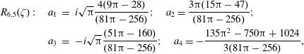 $$\begin{eqnarray}\displaystyle R_{6,5}(\unicode[STIX]{x1D701}):\quad a_{1} & = & \displaystyle i\sqrt{\unicode[STIX]{x03C0}}\frac{4(9\unicode[STIX]{x03C0}-28)}{(81\unicode[STIX]{x03C0}-256)};\quad a_{2}=\frac{3\unicode[STIX]{x03C0}(15\unicode[STIX]{x03C0}-47)}{(81\unicode[STIX]{x03C0}-256)};\nonumber\\ \displaystyle a_{3} & = & \displaystyle -i\sqrt{\unicode[STIX]{x03C0}}\frac{(51\unicode[STIX]{x03C0}-160)}{(81\unicode[STIX]{x03C0}-256)};\quad a_{4}=-\frac{135\unicode[STIX]{x03C0}^{2}-750\unicode[STIX]{x03C0}+1024}{3(81\unicode[STIX]{x03C0}-256)},\end{eqnarray}$$
 $$\begin{eqnarray}\displaystyle & \displaystyle R_{6,6}(\unicode[STIX]{x1D701}):\quad a_{1}=i\sqrt{\unicode[STIX]{x03C0}}\frac{(45\unicode[STIX]{x03C0}-152)}{(45\unicode[STIX]{x03C0}-128)};\quad a_{2}=\frac{(159\unicode[STIX]{x03C0}-512)}{(45\unicode[STIX]{x03C0}-128)}; & \displaystyle \nonumber\\ \displaystyle & \displaystyle a_{3}=-9i\sqrt{\unicode[STIX]{x03C0}}\frac{(5\unicode[STIX]{x03C0}-16)}{(45\unicode[STIX]{x03C0}-128)}; & \displaystyle\end{eqnarray}$$
 $$\begin{eqnarray}\displaystyle & \displaystyle R_{6,7}(\unicode[STIX]{x1D701}):\quad a_{1}=-i\sqrt{\unicode[STIX]{x03C0}}{\textstyle \frac{7}{8}};\quad a_{2}=4-{\textstyle \frac{105}{64}}\unicode[STIX]{x03C0}; & \displaystyle\end{eqnarray}$$
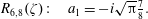 $$\begin{eqnarray}\displaystyle & \displaystyle R_{6,8}(\unicode[STIX]{x1D701}):\quad a_{1}=-i\sqrt{\unicode[STIX]{x03C0}}{\textstyle \frac{7}{8}}. & \displaystyle\end{eqnarray}$$
A.3 Seven-pole approximants of
$R(\unicode[STIX]{x1D701})$

 $$\begin{eqnarray}R_{7}(\unicode[STIX]{x1D701})=\frac{1+a_{1}\unicode[STIX]{x1D701}+a_{2}\unicode[STIX]{x1D701}^{2}+a_{3}\unicode[STIX]{x1D701}^{3}+a_{4}\unicode[STIX]{x1D701}^{4}+a_{5}\unicode[STIX]{x1D701}^{5}}{1+b_{1}\unicode[STIX]{x1D701}+b_{2}\unicode[STIX]{x1D701}^{2}+b_{3}\unicode[STIX]{x1D701}^{3}+b_{4}\unicode[STIX]{x1D701}^{4}+b_{5}\unicode[STIX]{x1D701}^{5}+b_{6}\unicode[STIX]{x1D701}^{6}+b_{7}\unicode[STIX]{x1D701}^{7}},\end{eqnarray}$$
and the procedure of matching with asymptotic expansion yields
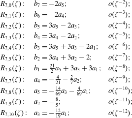 $$\begin{eqnarray}\displaystyle \begin{array}{@{}lll@{}}R_{7,0}(\unicode[STIX]{x1D701}):\quad & b_{7}=-2a_{5};\quad & o(\unicode[STIX]{x1D701}^{-2});\\ R_{7,1}(\unicode[STIX]{x1D701}):\quad & b_{6}=-2a_{4};\quad & o(\unicode[STIX]{x1D701}^{-3});\\ R_{7,2}(\unicode[STIX]{x1D701}):\quad & b_{5}=3a_{5}-2a_{3};\quad & o(\unicode[STIX]{x1D701}^{-4});\\ R_{7,3}(\unicode[STIX]{x1D701}):\quad & b_{4}=3a_{4}-2a_{2};\quad & o(\unicode[STIX]{x1D701}^{-5});\\ R_{7,4}(\unicode[STIX]{x1D701}):\quad & b_{3}=3a_{5}+3a_{3}-2a_{1};\quad & o(\unicode[STIX]{x1D701}^{-6});\\ R_{7,5}(\unicode[STIX]{x1D701}):\quad & b_{2}=3a_{4}+3a_{2}-2;\quad & o(\unicode[STIX]{x1D701}^{-7});\\ R_{7,6}(\unicode[STIX]{x1D701}):\quad & b_{1}=\frac{21}{2}a_{5}+3a_{3}+3a_{1};\quad & o(\unicode[STIX]{x1D701}^{-8});\\ R_{7,7}(\unicode[STIX]{x1D701}):\quad & a_{4}=-\frac{4}{21}-\frac{2}{7}a_{2};\quad & o(\unicode[STIX]{x1D701}^{-9});\\ R_{7,8}(\unicode[STIX]{x1D701}):\quad & a_{5}=-\frac{14}{69}a_{3}-\frac{4}{69}a_{1};\quad & o(\unicode[STIX]{x1D701}^{-10});\\ R_{7,9}(\unicode[STIX]{x1D701}):\quad & a_{2}=-\frac{8}{5};\quad & o(\unicode[STIX]{x1D701}^{-11});\\ R_{7,10}(\unicode[STIX]{x1D701}):\quad & a_{3}=-\frac{12}{19}a_{1};\quad & o(\unicode[STIX]{x1D701}^{-12}).\end{array} & & \displaystyle\end{eqnarray}$$
The
 $R_{7,11}(\unicode[STIX]{x1D701})$
is not defined because it would require
$R_{7,11}(\unicode[STIX]{x1D701})$
is not defined because it would require
 $a_{1}\rightarrow \infty$
. Matching with the power series is performed according to
$a_{1}\rightarrow \infty$
. Matching with the power series is performed according to
 $$\begin{eqnarray}\displaystyle R_{7,0}(\unicode[STIX]{x1D701}) & = & \displaystyle 1+i\sqrt{\unicode[STIX]{x03C0}}\unicode[STIX]{x1D701}-2\unicode[STIX]{x1D701}^{2}-i\sqrt{\unicode[STIX]{x03C0}}\unicode[STIX]{x1D701}^{3}+\frac{4}{3}\unicode[STIX]{x1D701}^{4}\nonumber\\ \displaystyle & & \displaystyle +\,i\frac{\sqrt{\unicode[STIX]{x03C0}}}{2}\unicode[STIX]{x1D701}^{5}-\frac{8}{15}\unicode[STIX]{x1D701}^{6}-i\frac{\sqrt{\unicode[STIX]{x03C0}}}{6}\unicode[STIX]{x1D701}^{7}+\frac{16}{105}\unicode[STIX]{x1D701}^{8}+i\frac{\sqrt{\unicode[STIX]{x03C0}}}{24}\unicode[STIX]{x1D701}^{9}-\frac{32}{945}\unicode[STIX]{x1D701}^{10}-i\frac{\sqrt{\unicode[STIX]{x03C0}}}{120}\unicode[STIX]{x1D701}^{11};\nonumber\\ \displaystyle & \vdots & \displaystyle \nonumber\\ \displaystyle R_{7,10}(\unicode[STIX]{x1D701}) & = & \displaystyle 1+i\sqrt{\unicode[STIX]{x03C0}}\unicode[STIX]{x1D701}.\end{eqnarray}$$
The results are
 $$\begin{eqnarray}\displaystyle R_{7,0}(\unicode[STIX]{x1D701}):\quad a_{1} & = & \displaystyle -i0.8324695834;\quad a_{2}=-0.4049799755;\nonumber\\ \displaystyle a_{3} & = & \displaystyle i0.1121082796;\quad a_{4}=0.01799681258;\nonumber\\ \displaystyle a_{5} & = & \displaystyle -i0.001293708127;\quad b_{1}=-i2.604923434;\nonumber\\ \displaystyle b_{2} & = & \displaystyle -3.022086548;\quad b_{3}=i2.031224201;\nonumber\\ \displaystyle b_{4} & = & \displaystyle 0.8578481138;\quad b_{5}=-i0.2288461173;\nonumber\\ \displaystyle b_{6} & = & \displaystyle -0.035945334608,\end{eqnarray}$$
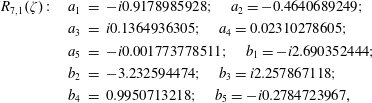 $$\begin{eqnarray}\displaystyle R_{7,1}(\unicode[STIX]{x1D701}):\quad a_{1} & = & \displaystyle -i0.9178985928;\quad a_{2}=-0.4640689249;\nonumber\\ \displaystyle a_{3} & = & \displaystyle i0.1364936305;\quad a_{4}=0.02310278605;\nonumber\\ \displaystyle a_{5} & = & \displaystyle -i0.001773778511;\quad b_{1}=-i2.690352444;\nonumber\\ \displaystyle b_{2} & = & \displaystyle -3.232594474;\quad b_{3}=i2.257867118;\nonumber\\ \displaystyle b_{4} & = & \displaystyle 0.9950713218;\quad b_{5}=-i0.2784723967,\end{eqnarray}$$
 $$\begin{eqnarray}\displaystyle R_{7,2}(\unicode[STIX]{x1D701}):\quad a_{1} & = & \displaystyle -i1.010198516;\quad a_{2}=-0.5369471092;\nonumber\\ \displaystyle a_{3} & = & \displaystyle i0.1677974137;\quad a_{4}=0.03023595150;\nonumber\\ \displaystyle a_{5} & = & \displaystyle -i0.002497479595;\quad b_{1}=-i2.782652367;\nonumber\\ \displaystyle b_{2} & = & \displaystyle -3.469070012;\quad b_{3}=i2.523713033;\nonumber\\ \displaystyle b_{4} & = & \displaystyle 1.164050381,\end{eqnarray}$$
 $$\begin{eqnarray}\displaystyle R_{7,3}(\unicode[STIX]{x1D701}):\quad a_{1} & = & \displaystyle -i1.109722119;\quad a_{2}=-0.6261744648;\nonumber\\ \displaystyle a_{3} & = & \displaystyle i0.2086297926;\quad a_{4}=0.04033869308;\nonumber\\ \displaystyle a_{5} & = & \displaystyle -i0.003624122579;\quad b_{1}=-i2.882175970;\nonumber\\ \displaystyle b_{2} & = & \displaystyle -3.734698361;\quad b_{3}=i2.836312196,\end{eqnarray}$$
 $$\begin{eqnarray}\displaystyle R_{7,4}(\unicode[STIX]{x1D701}):\quad a_{1} & = & \displaystyle -i1.216585782;\quad a_{2}=-0.7344009695;\nonumber\\ \displaystyle a_{3} & = & \displaystyle i0.2623273358;\quad a_{4}=0.05488528512;\nonumber\\ \displaystyle a_{5} & = & \displaystyle -i0.005440857949;\quad b_{1}=-i2.989039633;\nonumber\\ \displaystyle b_{2} & = & \displaystyle -4.032335777,\end{eqnarray}$$
 $$\begin{eqnarray}\displaystyle R_{7,5}(\unicode[STIX]{x1D701}):\quad a_{1} & = & \displaystyle -i1.330549030;\quad a_{2}=-0.8640648164;\nonumber\\ \displaystyle a_{3} & = & \displaystyle i0.3328884746;\quad a_{4}=0.07606674237;\nonumber\\ \displaystyle a_{5} & = & \displaystyle -i0.008482851988;\quad b_{1}=-i3.103002881,\end{eqnarray}$$
 $$\begin{eqnarray}\displaystyle R_{7,6}(\unicode[STIX]{x1D701}):\quad a_{1} & = & \displaystyle -i1.450931895;\quad a_{2}=-1.016999244;\nonumber\\ \displaystyle a_{3} & = & \displaystyle i0.4247000792;\quad a_{4}=0.1068986701;\nonumber\\ \displaystyle a_{5} & = & \displaystyle -i0.01378002846,\end{eqnarray}$$
 $$\begin{eqnarray}\displaystyle R_{7,7}(\unicode[STIX]{x1D701}):\quad a_{1} & = & \displaystyle -i1.576631991;\quad a_{2}=-1.194087585;\nonumber\\ \displaystyle a_{3} & = & \displaystyle i0.5420816788;\quad a_{5}=-i0.02337475294.\end{eqnarray}$$
We later found that the most precise (power-series) closure on the sixth-order moment is a dynamic closure constructed with approximant
 $R_{7,5}(\unicode[STIX]{x1D701})$
, and therefore, starting with this approximant, we also provide analytic coefficients. The results are
$R_{7,5}(\unicode[STIX]{x1D701})$
, and therefore, starting with this approximant, we also provide analytic coefficients. The results are
 $$\begin{eqnarray}\displaystyle R_{7,5}(\unicode[STIX]{x1D701}):\quad a_{1} & = & \displaystyle i\frac{2(3375\unicode[STIX]{x03C0}^{3}-24525\unicode[STIX]{x03C0}^{2}+54168\unicode[STIX]{x03C0}-32768)}{15(450\unicode[STIX]{x03C0}^{2}-2799\unicode[STIX]{x03C0}+4352)\sqrt{\unicode[STIX]{x03C0}}};\nonumber\\ \displaystyle a_{2} & = & \displaystyle \frac{(6030\unicode[STIX]{x03C0}^{2}-37197\unicode[STIX]{x03C0}+57344)}{30(450\unicode[STIX]{x03C0}^{2}-2799\unicode[STIX]{x03C0}+4352)};\nonumber\\ \displaystyle a_{3} & = & \displaystyle i\frac{3(600\unicode[STIX]{x03C0}^{2}-3805\unicode[STIX]{x03C0}+6032)\sqrt{\unicode[STIX]{x03C0}}}{10(450\unicode[STIX]{x03C0}^{2}-2799\unicode[STIX]{x03C0}+4352)};\quad a_{4}=\frac{(1545\unicode[STIX]{x03C0}^{2}-9743\unicode[STIX]{x03C0}+15360)}{5(450\unicode[STIX]{x03C0}^{2}-2799\unicode[STIX]{x03C0}+4352)};\nonumber\\ \displaystyle a_{5} & = & \displaystyle i\frac{(10800\unicode[STIX]{x03C0}^{3}-120915\unicode[STIX]{x03C0}^{2}+440160\unicode[STIX]{x03C0}-524288)}{90(450\unicode[STIX]{x03C0}^{2}-2799\unicode[STIX]{x03C0}+4352)\sqrt{\unicode[STIX]{x03C0}}};\nonumber\\ \displaystyle b_{1} & := & \displaystyle -i\frac{(7065\unicode[STIX]{x03C0}^{2}-43056\unicode[STIX]{x03C0}+65536)}{15(450\unicode[STIX]{x03C0}^{2}-2799\unicode[STIX]{x03C0}+4352)\sqrt{\unicode[STIX]{x03C0}}},\end{eqnarray}$$
 $$\begin{eqnarray}\displaystyle R_{7,6}(\unicode[STIX]{x1D701}):\quad a_{1} & = & \displaystyle i\sqrt{\unicode[STIX]{x03C0}}\frac{(1350\unicode[STIX]{x03C0}^{2}-8601\unicode[STIX]{x03C0}+13696)}{2(675\unicode[STIX]{x03C0}^{2}-4728\unicode[STIX]{x03C0}+8192)};\nonumber\\ \displaystyle a_{2} & = & \displaystyle -\frac{3(135\unicode[STIX]{x03C0}-424)\unicode[STIX]{x03C0}}{2(675\unicode[STIX]{x03C0}^{2}-4728\unicode[STIX]{x03C0}+8192)};\nonumber\\ \displaystyle a_{3} & = & \displaystyle i\sqrt{\unicode[STIX]{x03C0}}\frac{(1800\unicode[STIX]{x03C0}^{2}-10707\unicode[STIX]{x03C0}+15872)}{2(675\unicode[STIX]{x03C0}^{2}-4728\unicode[STIX]{x03C0}+8192)};\nonumber\\ \displaystyle a_{4} & = & \displaystyle \frac{(7065\unicode[STIX]{x03C0}^{2}-43056\unicode[STIX]{x03C0}+65536)}{6(675\unicode[STIX]{x03C0}^{2}-4728\unicode[STIX]{x03C0}+8192)};\nonumber\\ \displaystyle a_{5} & = & \displaystyle -i\sqrt{\unicode[STIX]{x03C0}}\frac{(450\unicode[STIX]{x03C0}^{2}-2799\unicode[STIX]{x03C0}+4352)}{(675\unicode[STIX]{x03C0}^{2}-4728\unicode[STIX]{x03C0}+8192)},\end{eqnarray}$$
 $$\begin{eqnarray}\displaystyle R_{7,7}(\unicode[STIX]{x1D701}):\quad a_{1} & = & \displaystyle i\frac{(675\unicode[STIX]{x03C0}^{2}-3432\unicode[STIX]{x03C0}+4096)}{3(-704+225\unicode[STIX]{x03C0})\sqrt{\unicode[STIX]{x03C0}}};\nonumber\\ \displaystyle a_{2} & = & \displaystyle \frac{(1545\unicode[STIX]{x03C0}-4864)}{3(-704+225\unicode[STIX]{x03C0})};\nonumber\\ \displaystyle a_{3} & = & \displaystyle i\frac{4(225\unicode[STIX]{x03C0}^{2}-2010\unicode[STIX]{x03C0}+4096)}{3(-704+225\unicode[STIX]{x03C0})\sqrt{\unicode[STIX]{x03C0}}};\nonumber\\ \displaystyle a_{5} & = & \displaystyle -i\frac{2(675\unicode[STIX]{x03C0}^{2}-4728\unicode[STIX]{x03C0}+8192)}{9(-704+225\unicode[STIX]{x03C0})\sqrt{\unicode[STIX]{x03C0}}},\end{eqnarray}$$
 $$\begin{eqnarray}\displaystyle R_{7,8}(\unicode[STIX]{x1D701}):\quad a_{1} & = & \displaystyle -i\sqrt{\unicode[STIX]{x03C0}}\frac{3(25\unicode[STIX]{x03C0}-72)}{256-75\unicode[STIX]{x03C0}};\quad a_{2}=-\frac{335\unicode[STIX]{x03C0}-1024}{256-75\unicode[STIX]{x03C0}};\nonumber\\ \displaystyle a_{3} & = & \displaystyle i\sqrt{\unicode[STIX]{x03C0}}\frac{5(165\unicode[STIX]{x03C0}-512)}{4(256-75\unicode[STIX]{x03C0})},\end{eqnarray}$$
 $$\begin{eqnarray}\displaystyle R_{7,9}(\unicode[STIX]{x1D701}):\quad a_{1} & = & \displaystyle -i\frac{32-5\unicode[STIX]{x03C0}}{5\sqrt{\unicode[STIX]{x03C0}}};\quad a_{3}=i\frac{1024-275\unicode[STIX]{x03C0}}{100\sqrt{\unicode[STIX]{x03C0}}},\end{eqnarray}$$
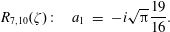 $$\begin{eqnarray}\displaystyle R_{7,10}(\unicode[STIX]{x1D701}):\quad a_{1} & = & \displaystyle -i\sqrt{\unicode[STIX]{x03C0}}\frac{19}{16}.\end{eqnarray}$$
A.4 Eight-pole approximants of
$R(\unicode[STIX]{x1D701})$

 $$\begin{eqnarray}R_{8}(\unicode[STIX]{x1D701})=\frac{1+a_{1}\unicode[STIX]{x1D701}+a_{2}\unicode[STIX]{x1D701}^{2}+a_{3}\unicode[STIX]{x1D701}^{3}+a_{4}\unicode[STIX]{x1D701}^{4}+a_{5}\unicode[STIX]{x1D701}^{5}+a_{6}\unicode[STIX]{x1D701}^{6}}{1+b_{1}\unicode[STIX]{x1D701}+b_{2}\unicode[STIX]{x1D701}^{2}+b_{3}\unicode[STIX]{x1D701}^{3}+b_{4}\unicode[STIX]{x1D701}^{4}+b_{5}\unicode[STIX]{x1D701}^{5}+b_{6}\unicode[STIX]{x1D701}^{6}+b_{7}\unicode[STIX]{x1D701}^{7}+b_{8}\unicode[STIX]{x1D701}^{8}},\end{eqnarray}$$
and the procedure of matching with the asymptotic expansion step by step
 $$\begin{eqnarray}R(\unicode[STIX]{x1D701})=-\frac{1}{2\unicode[STIX]{x1D701}^{2}}-\frac{3}{4\unicode[STIX]{x1D701}^{4}}-\frac{15}{8\unicode[STIX]{x1D701}^{6}}-\frac{105}{16\unicode[STIX]{x1D701}^{8}}-\frac{945}{32\unicode[STIX]{x1D701}^{10}}-\frac{10395}{64\unicode[STIX]{x1D701}^{12}}-\frac{135135}{128\unicode[STIX]{x1D701}^{14}}\cdots \,;\quad |\unicode[STIX]{x1D701}|\gg 1\end{eqnarray}$$
yields the following table
 $$\begin{eqnarray}\begin{array}{@{}lll@{}}\displaystyle R_{8,0}(\unicode[STIX]{x1D701}):\quad & b_{8}=-2a_{6};\quad & o(\unicode[STIX]{x1D701}^{-2});\\ \displaystyle R_{8,1}(\unicode[STIX]{x1D701}):\quad & b_{7}=-2a_{5};\quad & o(\unicode[STIX]{x1D701}^{-3});\\ \displaystyle R_{8,2}(\unicode[STIX]{x1D701}):\quad & b_{6}=3a_{6}-2a_{4};\quad & o(\unicode[STIX]{x1D701}^{-4});\\ \displaystyle R_{8,3}(\unicode[STIX]{x1D701}):\quad & b_{5}=3a_{5}-2a_{3};\quad & o(\unicode[STIX]{x1D701}^{-5});\\ \displaystyle R_{8,4}(\unicode[STIX]{x1D701}):\quad & b_{4}=3a_{6}+3a_{4}-2a_{2};\quad & o(\unicode[STIX]{x1D701}^{-6});\\ \displaystyle R_{8,5}(\unicode[STIX]{x1D701}):\quad & b_{3}=3a_{5}+3a_{3}-2a_{1};\quad & o(\unicode[STIX]{x1D701}^{-7});\\ \displaystyle R_{8,6}(\unicode[STIX]{x1D701}):\quad & b_{2}={\textstyle \frac{21}{2}}a_{6}+3a_{4}+3a_{2}-2;\quad & o(\unicode[STIX]{x1D701}^{-8});\\ \displaystyle R_{8,7}(\unicode[STIX]{x1D701}):\quad & b_{1}={\textstyle \frac{21}{2}}a_{5}+3a_{3}+3a_{1};\quad & o(\unicode[STIX]{x1D701}^{-9});\\ \displaystyle R_{8,8}(\unicode[STIX]{x1D701}):\quad & a_{6}=-{\textstyle \frac{14}{69}}a_{4}-{\textstyle \frac{4}{69}}a_{2}-{\textstyle \frac{8}{207}};\quad & o(\unicode[STIX]{x1D701}^{-10});\\ \displaystyle R_{8,9}(\unicode[STIX]{x1D701}):\quad & a_{5}=-{\textstyle \frac{14}{69}}a_{3}-{\textstyle \frac{4}{69}}a_{1};\quad & o(\unicode[STIX]{x1D701}^{-11});\\ \displaystyle R_{8,10}(\unicode[STIX]{x1D701}):\quad & a_{4}=-{\textstyle \frac{12}{19}}a_{2}-{\textstyle \frac{212}{285}};\quad & o(\unicode[STIX]{x1D701}^{-12});\\ \displaystyle R_{8,11}(\unicode[STIX]{x1D701}):\quad & a_{3}=-{\textstyle \frac{12}{19}}a_{1};\quad & o(\unicode[STIX]{x1D701}^{-13});\\ \displaystyle R_{8,12}(\unicode[STIX]{x1D701}):\quad & a_{2}=-{\textstyle \frac{94}{35}};\quad & o(\unicode[STIX]{x1D701}^{-14});\\ \displaystyle R_{8,13}(\unicode[STIX]{x1D701}):\quad & a_{1}=0;\quad & o(\unicode[STIX]{x1D701}^{-15}),\end{array}\end{eqnarray}$$
where the approximant
 $R_{8,13}(\unicode[STIX]{x1D701})$
is not well behaved and is eliminated. Matching with the power series is performed according to
$R_{8,13}(\unicode[STIX]{x1D701})$
is not well behaved and is eliminated. Matching with the power series is performed according to
 $$\begin{eqnarray}\displaystyle R_{8,0}(\unicode[STIX]{x1D701}) & = & \displaystyle 1+i\sqrt{\unicode[STIX]{x03C0}}\unicode[STIX]{x1D701}-2\unicode[STIX]{x1D701}^{2}-i\sqrt{\unicode[STIX]{x03C0}}\unicode[STIX]{x1D701}^{3}+\frac{4}{3}\unicode[STIX]{x1D701}^{4}\nonumber\\ \displaystyle & & \displaystyle \quad +\,i\frac{\sqrt{\unicode[STIX]{x03C0}}}{2}\unicode[STIX]{x1D701}^{5}-\frac{8}{15}\unicode[STIX]{x1D701}^{6}-i\frac{\sqrt{\unicode[STIX]{x03C0}}}{6}\unicode[STIX]{x1D701}^{7}+\frac{16}{105}\unicode[STIX]{x1D701}^{8}+i\frac{\sqrt{\unicode[STIX]{x03C0}}}{24}\unicode[STIX]{x1D701}^{9}-\frac{32}{945}\unicode[STIX]{x1D701}^{10}\nonumber\\ \displaystyle & & \displaystyle \quad -\,i\frac{\sqrt{\unicode[STIX]{x03C0}}}{120}\unicode[STIX]{x1D701}^{11}+\frac{64}{10395}\unicode[STIX]{x1D701}^{12}+i\frac{\sqrt{\unicode[STIX]{x03C0}}}{720}\unicode[STIX]{x1D701}^{13};\quad |\unicode[STIX]{x1D701}|\ll 1;\nonumber\\ \displaystyle & \vdots & \displaystyle \nonumber\\ \displaystyle R_{8,12}(\unicode[STIX]{x1D701}) & = & \displaystyle 1+i\sqrt{\unicode[STIX]{x03C0}}\unicode[STIX]{x1D701}.\end{eqnarray}$$
Such high-order Padé approximants are very precise, and to retain the accuracy, we provide solutions with 16 correct significant digits (even though this is actually not necessary and 10 digits is still fully sufficient). The approximant
 $R_{8,3}(\unicode[STIX]{x1D701})$
is a bit special, since its corresponding
$R_{8,3}(\unicode[STIX]{x1D701})$
is a bit special, since its corresponding
 $Z_{8,3}(\unicode[STIX]{x1D701})$
should be the approximant that is used in the WHAMP code. This is inferred from a sentence on page 12 of the WHAMP manual (Rönnmark Reference Rönnmark1982), where it is stated that an eight-pole approximant was derived, using 10 equations from the power-series expansion and 6 equations from the asymptotic-series expansion. However, the Padé coefficients in the WHAMP manual are given in a different form than we use here, and an alternative Padé approximation is used where for example an eight-pole approximant is given by
$Z_{8,3}(\unicode[STIX]{x1D701})$
should be the approximant that is used in the WHAMP code. This is inferred from a sentence on page 12 of the WHAMP manual (Rönnmark Reference Rönnmark1982), where it is stated that an eight-pole approximant was derived, using 10 equations from the power-series expansion and 6 equations from the asymptotic-series expansion. However, the Padé coefficients in the WHAMP manual are given in a different form than we use here, and an alternative Padé approximation is used where for example an eight-pole approximant is given by
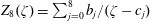 $Z_{8}(\unicode[STIX]{x1D701})=\sum _{j=0}^{8}b_{j}/(\unicode[STIX]{x1D701}-c_{j})$
, and the coefficients
$Z_{8}(\unicode[STIX]{x1D701})=\sum _{j=0}^{8}b_{j}/(\unicode[STIX]{x1D701}-c_{j})$
, and the coefficients
 $b_{j},c_{j}$
are obtained. We did not bother to re-derive the coefficients in that form, instead, we compare the precision of various approximants in § 3.5.
$b_{j},c_{j}$
are obtained. We did not bother to re-derive the coefficients in that form, instead, we compare the precision of various approximants in § 3.5.
 $$\begin{eqnarray}\displaystyle R_{8,0}(\unicode[STIX]{x1D701}):\quad a_{1} & = & \displaystyle -i0.9690248260959390;\quad a_{2}=-0.5368540729623971;\nonumber\\ \displaystyle a_{3} & = & \displaystyle i0.1799961104391385;\nonumber\\ \displaystyle a_{4} & = & \displaystyle 0.03849976076674387;\quad a_{5}=-i0.004838817622209550;\nonumber\\ \displaystyle a_{6} & = & \displaystyle -0.0002789155539114067;\nonumber\\ \displaystyle b_{1} & = & \displaystyle -i2.741478677001455;\quad b_{2}=-3.395998511188985;\nonumber\\ \displaystyle b_{3} & = & \displaystyle i2.488743246168061;\nonumber\\ \displaystyle b_{4} & = & \displaystyle 1.183496393867702;\quad b_{5}=-i0.3752177277401555;\nonumber\\ \displaystyle b_{6} & = & \displaystyle -0.07776565572655091;\nonumber\\ \displaystyle b_{7} & = & \displaystyle i0.009681326596560459,\end{eqnarray}$$
 $$\begin{eqnarray}\displaystyle R_{8,1}(\unicode[STIX]{x1D701}):\quad a_{1} & = & \displaystyle -i1.045465281824923;\quad a_{2}=-0.6004884272987368;\nonumber\\ \displaystyle a_{3} & = & \displaystyle i0.2109529643239577;\nonumber\\ \displaystyle a_{4} & = & \displaystyle 0.04706936874656537;\quad a_{5}=-i0.006214502177680713;\nonumber\\ \displaystyle a_{6} & = & \displaystyle -0.0003778071927517807;\nonumber\\ \displaystyle b_{1} & = & \displaystyle -i2.817919132730439;\quad b_{2}=-3.595120045647135;\nonumber\\ \displaystyle b_{3} & = & \displaystyle i2.719752919143475;\nonumber\\ \displaystyle b_{4} & = & \displaystyle 1.338764097514731;\quad b_{5}=-i0.4407920285051489;\nonumber\\ \displaystyle b_{6} & = & \displaystyle -0.0952587572277513,\end{eqnarray}$$
 $$\begin{eqnarray}\displaystyle R_{8,2}(\unicode[STIX]{x1D701}):\quad a_{1} & = & \displaystyle -i1.127283578226963;\quad a_{2}=-0.6755893264302076;\nonumber\\ \displaystyle a_{3} & = & \displaystyle i0.2489222931730291;\nonumber\\ \displaystyle a_{4} & = & \displaystyle 0.05823704506630824;\quad a_{5}=-i0.008104732774508430;\nonumber\\ \displaystyle a_{6} & = & \displaystyle -0.0005229347287036976;\nonumber\\ \displaystyle b_{1} & = & \displaystyle -i2.899737429132479;\quad b_{2}=-3.815240099310931;\nonumber\\ \displaystyle b_{3} & = & \displaystyle i2.984238291966390;\nonumber\\ \displaystyle b_{4} & = & \displaystyle 1.523498938607364;\quad b_{5}=-i0.5222070688557393,\end{eqnarray}$$
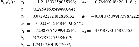 $$\begin{eqnarray}\displaystyle R_{8,3}(\unicode[STIX]{x1D701}):\quad a_{1} & = & \displaystyle -i1.214803859035098;\quad a_{2}=-0.7640021842041184;\nonumber\\ \displaystyle a_{3} & = & \displaystyle i0.2959160549490394;\nonumber\\ \displaystyle a_{4} & = & \displaystyle 0.07292272182826132;\quad a_{5}=-i0.01075099173987222;\nonumber\\ \displaystyle a_{6} & = & \displaystyle -0.0007415148441966772;\nonumber\\ \displaystyle b_{1} & = & \displaystyle -i2.987257709940614;\quad b_{2}=-4.058778615835553;\nonumber\\ \displaystyle b_{3} & = & \displaystyle i3.287852273584013;\nonumber\\ \displaystyle b_{4} & = & \displaystyle 1.744375011977697,\end{eqnarray}$$
 $$\begin{eqnarray}\displaystyle R_{8,4}(\unicode[STIX]{x1D701}):\quad a_{1} & = & \displaystyle -i1.308257217643640;\quad a_{2}=-0.8677094433207613;\nonumber\\ \displaystyle a_{3} & = & \displaystyle i0.3544341617560842;\nonumber\\ \displaystyle a_{4} & = & \displaystyle 0.09241987665571996;\quad a_{5}=-i0.01452077809048251;\nonumber\\ \displaystyle a_{6} & = & \displaystyle -0.001080201271194285;\nonumber\\ \displaystyle b_{1} & = & \displaystyle -i3.080711068549157;\quad b_{2}=-4.328127640297961;\nonumber\\ \displaystyle b_{3} & = & \displaystyle i3.636872378820012,\end{eqnarray}$$
 $$\begin{eqnarray}\displaystyle R_{8,5}(\unicode[STIX]{x1D701}):\quad a_{1} & = & \displaystyle -i1.407720282460896;\quad a_{2}=-0.9887147938014795;\nonumber\\ \displaystyle a_{3} & = & \displaystyle i0.4274799329839440;\nonumber\\ \displaystyle a_{4} & = & \displaystyle 0.1185117574638203;\quad a_{5}=-i0.01997983676237579;\nonumber\\ \displaystyle a_{6} & = & \displaystyle -0.001621365678069347;\nonumber\\ \displaystyle b_{1} & = & \displaystyle -i3.180174133366412;\quad b_{2}=-4.625426683036889,\end{eqnarray}$$
 $$\begin{eqnarray}\displaystyle R_{8,6}(\unicode[STIX]{x1D701}):\quad a_{1} & = & \displaystyle -i1.513048776977928;\quad a_{2}=-1.128859520019374;\nonumber\\ \displaystyle a_{3} & = & \displaystyle i0.5184905792641649;\nonumber\\ \displaystyle a_{4} & = & \displaystyle 0.1535743993372947;\quad a_{5}=-i0.02799183221943639;\nonumber\\ \displaystyle a_{6} & = & \displaystyle -0.002514851707175031;\nonumber\\ \displaystyle b_{1} & = & \displaystyle -i3.285502627883444,\end{eqnarray}$$
 $$\begin{eqnarray}\displaystyle R_{8,7}(\unicode[STIX]{x1D701}):\quad a_{1} & = & \displaystyle -i1.623826833670546;\quad a_{2}=-1.289590935716420;\nonumber\\ \displaystyle a_{3} & = & \displaystyle i0.6311517791766421;\nonumber\\ \displaystyle a_{4} & = & \displaystyle 0.2006218487856471;\quad a_{5}=-i0.03983385915184296;\nonumber\\ \displaystyle a_{6} & = & \displaystyle -0.004041376481615575,\end{eqnarray}$$
 $$\begin{eqnarray}\displaystyle R_{8,8}(\unicode[STIX]{x1D701}):\quad a_{1} & = & \displaystyle -i1.739359630417800;\quad a_{2}=-1.471743639038102;\nonumber\\ \displaystyle a_{3} & = & \displaystyle i0.7691080574071934;\nonumber\\ \displaystyle a_{4} & = & \displaystyle 0.2632500611991985;\quad a_{5}=-i0.05724369164680910,\end{eqnarray}$$
 $$\begin{eqnarray}\displaystyle R_{8,9}(\unicode[STIX]{x1D701}):\quad a_{1} & = & \displaystyle -i1.858726543442496;\quad a_{2}=-1.675414915338742;\nonumber\\ \displaystyle a_{3} & = & \displaystyle i0.9356405409666494;\nonumber\\ \displaystyle a_{4} & = & \displaystyle 0.3458159069196990,\end{eqnarray}$$
and we provide analytic results for the last 3 approximants,
 $$\begin{eqnarray}\displaystyle R_{8,10}(\unicode[STIX]{x1D701}):\quad a_{1} & = & \displaystyle i\sqrt{\unicode[STIX]{x03C0}}\frac{175\unicode[STIX]{x03C0}-592}{175\unicode[STIX]{x03C0}-512};\quad a_{2}=\frac{955\unicode[STIX]{x03C0}-3072}{175\unicode[STIX]{x03C0}-512};\nonumber\\ \displaystyle a_{3} & = & \displaystyle i\sqrt{\unicode[STIX]{x03C0}}\frac{6144-1925\unicode[STIX]{x03C0}}{4(175\unicode[STIX]{x03C0}-512)};\end{eqnarray}$$
 $$\begin{eqnarray}\displaystyle R_{8,11}(\unicode[STIX]{x1D701}):\quad a_{1} & = & \displaystyle -i\sqrt{\unicode[STIX]{x03C0}}{\textstyle \frac{19}{16}};\quad a_{2}=6-{\textstyle \frac{665}{256}}\unicode[STIX]{x03C0};\end{eqnarray}$$
 $$\begin{eqnarray}\displaystyle R_{8,12}(\unicode[STIX]{x1D701}):\quad a_{1} & = & \displaystyle -i\sqrt{\unicode[STIX]{x03C0}}{\textstyle \frac{19}{16}}.\end{eqnarray}$$
We also provide analytic coefficients for
 $R_{8,6}(\unicode[STIX]{x1D701})$
, since this approximant can be used to construct the most precise dynamic closure for the seventh-order moment, which we will not do, however, an enthusiastic reader is encouraged to do the calculation as an exercise! The
$R_{8,6}(\unicode[STIX]{x1D701})$
, since this approximant can be used to construct the most precise dynamic closure for the seventh-order moment, which we will not do, however, an enthusiastic reader is encouraged to do the calculation as an exercise! The
 $R_{8,6}(\unicode[STIX]{x1D701})$
coefficients read
$R_{8,6}(\unicode[STIX]{x1D701})$
coefficients read
 $$\begin{eqnarray}\displaystyle R_{8,6}(\unicode[STIX]{x1D701}):\quad a_{1} & = & \displaystyle i\sqrt{\unicode[STIX]{x03C0}}\frac{(189000\unicode[STIX]{x03C0}^{3}-1707165\unicode[STIX]{x03C0}^{2}+5130216\unicode[STIX]{x03C0}-5128192)}{(189000\unicode[STIX]{x03C0}^{3}-1612215\unicode[STIX]{x03C0}^{2}+4534656\unicode[STIX]{x03C0}-4194304)};\nonumber\\ \displaystyle a_{2} & = & \displaystyle -\frac{2(46125\unicode[STIX]{x03C0}^{3}-715200\unicode[STIX]{x03C0}^{2}+3126720\unicode[STIX]{x03C0}-4194304)}{5(189000\unicode[STIX]{x03C0}^{3}-1612215\unicode[STIX]{x03C0}^{2}+4534656\unicode[STIX]{x03C0}-4194304)};\nonumber\\ \displaystyle a_{3} & = & \displaystyle i\sqrt{\unicode[STIX]{x03C0}}\frac{(378000\unicode[STIX]{x03C0}^{3}-3424725\unicode[STIX]{x03C0}^{2}+10324380\unicode[STIX]{x03C0}-10354688)}{5(189000\unicode[STIX]{x03C0}^{3}-1612215\unicode[STIX]{x03C0}^{2}+4534656\unicode[STIX]{x03C0}-4194304)};\nonumber\\ \displaystyle a_{4} & = & \displaystyle -\frac{(221400\unicode[STIX]{x03C0}^{3}-4788045\unicode[STIX]{x03C0}^{2}+23537664\unicode[STIX]{x03C0}-33554432)}{30(189000\unicode[STIX]{x03C0}^{3}-1612215\unicode[STIX]{x03C0}^{2}+4534656\unicode[STIX]{x03C0}-4194304)};\nonumber\\ \displaystyle a_{5} & = & \displaystyle i\sqrt{\unicode[STIX]{x03C0}}\frac{(252000\unicode[STIX]{x03C0}^{3}-2506275\unicode[STIX]{x03C0}^{2}+8286200\unicode[STIX]{x03C0}-9109504)}{5(189000\unicode[STIX]{x03C0}^{3}-1612215\unicode[STIX]{x03C0}^{2}+4534656\unicode[STIX]{x03C0}-4194304)};\nonumber\\ \displaystyle a_{6} & = & \displaystyle \frac{(1028700\unicode[STIX]{x03C0}^{3}-9863235\unicode[STIX]{x03C0}^{2}+31514112\unicode[STIX]{x03C0}-33554432)}{15(189000\unicode[STIX]{x03C0}^{3}-1612215\unicode[STIX]{x03C0}^{2}+4534656\unicode[STIX]{x03C0}-4194304)};\nonumber\\ \displaystyle b_{1} & = & \displaystyle -i\sqrt{\unicode[STIX]{x03C0}}\frac{6(15825\unicode[STIX]{x03C0}^{2}-99260\unicode[STIX]{x03C0}+155648)}{(189000\unicode[STIX]{x03C0}^{3}-1612215\unicode[STIX]{x03C0}^{2}+4534656\unicode[STIX]{x03C0}-4194304)}.\nonumber\\ \displaystyle & & \displaystyle\end{eqnarray}$$
We advise being very careful when evaluating the above analytic expressions, since for example when the default 10-digit precision is used in Maple, yields
 $a_{1}=-i0.63$
, whereas the correct value provided in (A 54) is
$a_{1}=-i0.63$
, whereas the correct value provided in (A 54) is
 $a_{1}=-i1.51$
.
$a_{1}=-i1.51$
.
Appendix B. Operator
$(\boldsymbol{E}+\frac{1}{c}\boldsymbol{v}\times \boldsymbol{B})\boldsymbol{\cdot }\unicode[STIX]{x1D735}_{v}f_{0}$
for gyrotropic
$f_{0}$
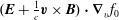

The magnetic field is transformed to the electric field with induction equation
 $\unicode[STIX]{x2202}\boldsymbol{B}^{(1)}/\unicode[STIX]{x2202}t=-c\unicode[STIX]{x1D735}\times \boldsymbol{E}^{(1)}$
that in Fourier space reads
$\unicode[STIX]{x2202}\boldsymbol{B}^{(1)}/\unicode[STIX]{x2202}t=-c\unicode[STIX]{x1D735}\times \boldsymbol{E}^{(1)}$
that in Fourier space reads
 $\unicode[STIX]{x1D714}\boldsymbol{B}^{(1)}=c\boldsymbol{k}\times \boldsymbol{E}^{(1)}$
. From now on, for the electric and magnetic field we drop the superscript (1), so in general
$\unicode[STIX]{x1D714}\boldsymbol{B}^{(1)}=c\boldsymbol{k}\times \boldsymbol{E}^{(1)}$
. From now on, for the electric and magnetic field we drop the superscript (1), so in general
 $$\begin{eqnarray}\displaystyle \boldsymbol{E}+\frac{1}{c}\boldsymbol{v}\times \boldsymbol{B} & = & \displaystyle \boldsymbol{E}+\frac{1}{\unicode[STIX]{x1D714}}\boldsymbol{v}\times (\boldsymbol{k}\times \boldsymbol{E})\nonumber\\ \displaystyle & = & \displaystyle \boldsymbol{E}+\frac{1}{\unicode[STIX]{x1D714}}\left(\boldsymbol{k}(\boldsymbol{v}\boldsymbol{\cdot }\boldsymbol{E})-\boldsymbol{E}(\boldsymbol{v}\boldsymbol{\cdot }\boldsymbol{k})\right)\nonumber\\ \displaystyle & = & \displaystyle \boldsymbol{E}\left(1-\frac{\boldsymbol{v}\boldsymbol{\cdot }\boldsymbol{k}}{\unicode[STIX]{x1D714}}\right)+\frac{\boldsymbol{k}}{\unicode[STIX]{x1D714}}(\boldsymbol{v}\boldsymbol{\cdot }\boldsymbol{E}).\end{eqnarray}$$
For any general vector
 $\boldsymbol{A}=(A_{x},A_{y},A_{z})$
, the expression
$\boldsymbol{A}=(A_{x},A_{y},A_{z})$
, the expression
 $$\begin{eqnarray}\displaystyle \boldsymbol{A}\boldsymbol{\cdot }\unicode[STIX]{x1D735}_{v}f_{0}=A_{x}\frac{\unicode[STIX]{x2202}f_{0}}{\unicode[STIX]{x2202}v_{x}}+A_{y}\frac{\unicode[STIX]{x2202}f_{0}}{\unicode[STIX]{x2202}v_{y}}+A_{z}\frac{\unicode[STIX]{x2202}f_{0}}{\unicode[STIX]{x2202}v_{z}}, & & \displaystyle\end{eqnarray}$$
so a general expression
 $$\begin{eqnarray}\displaystyle \left(\boldsymbol{E}+\frac{1}{c}\boldsymbol{v}\times \boldsymbol{B}\right)\boldsymbol{\cdot }\unicode[STIX]{x1D735}_{v}f_{0} & = & \displaystyle \left[E_{x}\left(1-\frac{\boldsymbol{v}\boldsymbol{\cdot }\boldsymbol{k}}{\unicode[STIX]{x1D714}}\right)+\frac{k_{x}}{\unicode[STIX]{x1D714}}(\boldsymbol{v}\boldsymbol{\cdot }\boldsymbol{E})\right]\frac{\unicode[STIX]{x2202}f_{0}}{\unicode[STIX]{x2202}v_{x}}\nonumber\\ \displaystyle & & \displaystyle +\,\left[E_{y}\left(1-\frac{\boldsymbol{v}\boldsymbol{\cdot }\boldsymbol{k}}{\unicode[STIX]{x1D714}}\right)+\frac{k_{y}}{\unicode[STIX]{x1D714}}(\boldsymbol{v}\boldsymbol{\cdot }\boldsymbol{E})\right]\frac{\unicode[STIX]{x2202}f_{0}}{\unicode[STIX]{x2202}v_{y}}\nonumber\\ \displaystyle & & \displaystyle +\,\left[E_{z}\left(1-\frac{\boldsymbol{v}\boldsymbol{\cdot }\boldsymbol{k}}{\unicode[STIX]{x1D714}}\right)+\frac{k_{z}}{\unicode[STIX]{x1D714}}(\boldsymbol{v}\boldsymbol{\cdot }\boldsymbol{E})\right]\frac{\unicode[STIX]{x2202}f_{0}}{\unicode[STIX]{x2202}v_{z}},\end{eqnarray}$$
and by straightforward grouping of electric field components together
 $$\begin{eqnarray}\displaystyle \left(\boldsymbol{E}+\frac{1}{c}\boldsymbol{v}\times \boldsymbol{B}\right)\boldsymbol{\cdot }\unicode[STIX]{x1D735}_{v}f_{0} & = & \displaystyle E_{x}\left[\left(1-\frac{v_{y}k_{y}+v_{z}k_{z}}{\unicode[STIX]{x1D714}}\right)\frac{\unicode[STIX]{x2202}f_{0}}{\unicode[STIX]{x2202}v_{x}}+\frac{v_{x}}{\unicode[STIX]{x1D714}}\left(k_{y}\frac{\unicode[STIX]{x2202}f_{0}}{\unicode[STIX]{x2202}v_{y}}+k_{z}\frac{\unicode[STIX]{x2202}f_{0}}{\unicode[STIX]{x2202}v_{z}}\right)\right]\nonumber\\ \displaystyle & & \displaystyle +\,E_{y}\left[\left(1-\frac{v_{x}k_{x}+v_{z}k_{z}}{\unicode[STIX]{x1D714}}\right)\frac{\unicode[STIX]{x2202}f_{0}}{\unicode[STIX]{x2202}v_{y}}+\frac{v_{y}}{\unicode[STIX]{x1D714}}\left(k_{x}\frac{\unicode[STIX]{x2202}f_{0}}{\unicode[STIX]{x2202}v_{x}}+k_{z}\frac{\unicode[STIX]{x2202}f_{0}}{\unicode[STIX]{x2202}v_{z}}\right)\right]\nonumber\\ \displaystyle & & \displaystyle +\,E_{z}\left[\left(1-\frac{v_{x}k_{x}+v_{y}k_{y}}{\unicode[STIX]{x1D714}}\right)\frac{\unicode[STIX]{x2202}f_{0}}{\unicode[STIX]{x2202}v_{z}}+\frac{v_{z}}{\unicode[STIX]{x1D714}}\left(k_{x}\frac{\unicode[STIX]{x2202}f_{0}}{\unicode[STIX]{x2202}v_{x}}+k_{y}\frac{\unicode[STIX]{x2202}f_{0}}{\unicode[STIX]{x2202}v_{y}}\right)\right].\nonumber\\ \displaystyle & & \displaystyle\end{eqnarray}$$
Since nothing was essentially calculated, the above expression is of general validity and correct for any distribution function
 $f_{0}$
. The expression simplifies by considering a gyrotropic
$f_{0}$
. The expression simplifies by considering a gyrotropic
 $f_{0}(v_{\bot },v_{\Vert })$
, that depends only on
$f_{0}(v_{\bot },v_{\Vert })$
, that depends only on
 $v_{\bot }=|\boldsymbol{v}_{\bot }|=\sqrt{v_{x}^{2}+v_{y}^{2}}$
, and which allows us to calculate
$v_{\bot }=|\boldsymbol{v}_{\bot }|=\sqrt{v_{x}^{2}+v_{y}^{2}}$
, and which allows us to calculate
 $$\begin{eqnarray}\displaystyle \frac{\unicode[STIX]{x2202}v_{\bot }}{\unicode[STIX]{x2202}v_{x}} & = & \displaystyle \frac{\sqrt{v_{x}^{2}+v_{y}^{2}}}{\unicode[STIX]{x2202}v_{x}}=\frac{v_{x}}{\sqrt{v_{x}^{2}+v_{y}^{2}}}=\frac{v_{x}}{v_{\bot }};\nonumber\\ \displaystyle \frac{\unicode[STIX]{x2202}f_{0}}{\unicode[STIX]{x2202}v_{x}} & = & \displaystyle \frac{\unicode[STIX]{x2202}v_{\bot }}{\unicode[STIX]{x2202}v_{x}}\frac{\unicode[STIX]{x2202}f_{0}}{\unicode[STIX]{x2202}v_{\bot }}=\frac{v_{x}}{v_{\bot }}\frac{\unicode[STIX]{x2202}f_{0}}{\unicode[STIX]{x2202}v_{\bot }};\quad \frac{\unicode[STIX]{x2202}f_{0}}{\unicode[STIX]{x2202}v_{y}}=\frac{\unicode[STIX]{x2202}v_{\bot }}{\unicode[STIX]{x2202}v_{y}}\frac{\unicode[STIX]{x2202}f_{0}}{\unicode[STIX]{x2202}v_{\bot }}=\frac{v_{y}}{v_{\bot }}\frac{\unicode[STIX]{x2202}f_{0}}{\unicode[STIX]{x2202}v_{\bot }}.\end{eqnarray}$$
Or in another words, in the cylindrical coordinate system the
 $f_{0}$
is
$f_{0}$
is
 $\unicode[STIX]{x1D719}$
independent and
$\unicode[STIX]{x1D719}$
independent and
 $\unicode[STIX]{x2202}f_{0}/\unicode[STIX]{x2202}\unicode[STIX]{x1D719}=0$
, so that the velocity gradient
$\unicode[STIX]{x2202}f_{0}/\unicode[STIX]{x2202}\unicode[STIX]{x1D719}=0$
, so that the velocity gradient
 $$\begin{eqnarray}\displaystyle \unicode[STIX]{x1D735}_{v}\,f_{0}=\left(\begin{array}{@{}c@{}}\frac{v_{x}}{v_{\bot }}\frac{\unicode[STIX]{x2202}}{\unicode[STIX]{x2202}v_{\bot }}\\ \frac{v_{y}}{v_{\bot }}\frac{\unicode[STIX]{x2202}}{\unicode[STIX]{x2202}v_{\bot }}\\ \frac{\unicode[STIX]{x2202}}{\unicode[STIX]{x2202}v_{\Vert }}\end{array}\right)\quad f_{0}=\left(\begin{array}{@{}c@{}}\cos \unicode[STIX]{x1D719}\frac{\unicode[STIX]{x2202}}{\unicode[STIX]{x2202}v_{\bot }}\\ \sin \unicode[STIX]{x1D719}\frac{\unicode[STIX]{x2202}}{\unicode[STIX]{x2202}v_{\bot }}\\ \frac{\unicode[STIX]{x2202}}{\unicode[STIX]{x2202}v_{\Vert }}\end{array}\right)f_{0}. & & \displaystyle\end{eqnarray}$$
This simplification for
 $f_{0}$
being gyrotropic therefore yields
$f_{0}$
being gyrotropic therefore yields
 $$\begin{eqnarray}\displaystyle \left(\boldsymbol{E}+\frac{1}{c}\boldsymbol{v}\times \boldsymbol{B}\right)\boldsymbol{\cdot }\unicode[STIX]{x1D735}_{v}f_{0} & = & \displaystyle E_{x}\left[\left(1-\frac{v_{\Vert }k_{\Vert }}{\unicode[STIX]{x1D714}}\right)\frac{v_{x}}{v_{\bot }}\frac{\unicode[STIX]{x2202}f_{0}}{\unicode[STIX]{x2202}v_{\bot }}+\frac{v_{x}}{\unicode[STIX]{x1D714}}k_{\Vert }\frac{\unicode[STIX]{x2202}f_{0}}{\unicode[STIX]{x2202}v_{\Vert }}\right]\nonumber\\ \displaystyle & & \displaystyle +\,E_{y}\left[\left(1-\frac{v_{\Vert }k_{\Vert }}{\unicode[STIX]{x1D714}}\right)\frac{v_{y}}{v_{\bot }}\frac{\unicode[STIX]{x2202}f_{0}}{\unicode[STIX]{x2202}v_{\bot }}+\frac{v_{y}}{\unicode[STIX]{x1D714}}k_{\Vert }\frac{\unicode[STIX]{x2202}f_{0}}{\unicode[STIX]{x2202}v_{\Vert }}\right]\nonumber\\ \displaystyle & & \displaystyle +\,E_{z}\left[\left(1-\frac{v_{x}k_{x}+v_{y}k_{y}}{\unicode[STIX]{x1D714}}\right)\frac{\unicode[STIX]{x2202}f_{0}}{\unicode[STIX]{x2202}v_{\Vert }}\right.\nonumber\\ \displaystyle & & \displaystyle \left.+\,\frac{v_{\Vert }}{\unicode[STIX]{x1D714}}\left(k_{x}\frac{v_{x}}{v_{\bot }}\frac{\unicode[STIX]{x2202}f_{0}}{\unicode[STIX]{x2202}v_{\bot }}+k_{y}\frac{v_{y}}{v_{\bot }}\frac{\unicode[STIX]{x2202}f_{0}}{\unicode[STIX]{x2202}v_{\bot }}\right)\right],\end{eqnarray}$$
that is conveniently rearranged as
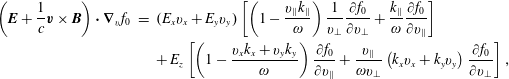 $$\begin{eqnarray}\displaystyle \left(\boldsymbol{E}+\frac{1}{c}\boldsymbol{v}\times \boldsymbol{B}\right)\boldsymbol{\cdot }\unicode[STIX]{x1D735}_{v}f_{0} & = & \displaystyle (E_{x}v_{x}+E_{y}v_{y})\left[\left(1-\frac{v_{\Vert }k_{\Vert }}{\unicode[STIX]{x1D714}}\right)\frac{1}{v_{\bot }}\frac{\unicode[STIX]{x2202}f_{0}}{\unicode[STIX]{x2202}v_{\bot }}+\frac{k_{\Vert }}{\unicode[STIX]{x1D714}}\frac{\unicode[STIX]{x2202}f_{0}}{\unicode[STIX]{x2202}v_{\Vert }}\right]\nonumber\\ \displaystyle & & \displaystyle +\,E_{z}\left[\left(1-\frac{v_{x}k_{x}+v_{y}k_{y}}{\unicode[STIX]{x1D714}}\right)\frac{\unicode[STIX]{x2202}f_{0}}{\unicode[STIX]{x2202}v_{\Vert }}+\frac{v_{\Vert }}{\unicode[STIX]{x1D714}v_{\bot }}\left(k_{x}v_{x}+k_{y}v_{y}\right)\frac{\unicode[STIX]{x2202}f_{0}}{\unicode[STIX]{x2202}v_{\bot }}\right],\nonumber\\ \displaystyle & & \displaystyle\end{eqnarray}$$
or alternatively as
 $$\begin{eqnarray}\displaystyle \left(\boldsymbol{E}+\frac{1}{c}\boldsymbol{v}\times \boldsymbol{B}\right)\boldsymbol{\cdot }\unicode[STIX]{x1D735}_{v}f_{0} & = & \displaystyle (E_{x}v_{x}+E_{y}v_{y})\left[\left(1-\frac{v_{\Vert }k_{\Vert }}{\unicode[STIX]{x1D714}}\right)\frac{1}{v_{\bot }}\frac{\unicode[STIX]{x2202}f_{0}}{\unicode[STIX]{x2202}v_{\bot }}+\frac{k_{\Vert }}{\unicode[STIX]{x1D714}}\frac{\unicode[STIX]{x2202}f_{0}}{\unicode[STIX]{x2202}v_{\Vert }}\right]\nonumber\\ \displaystyle & & \displaystyle +\,E_{z}\left[\frac{\unicode[STIX]{x2202}f_{0}}{\unicode[STIX]{x2202}v_{\Vert }}-\frac{v_{x}k_{x}+v_{y}k_{y}}{\unicode[STIX]{x1D714}}\left(\frac{\unicode[STIX]{x2202}f_{0}}{\unicode[STIX]{x2202}v_{\Vert }}-\frac{v_{\Vert }}{v_{\bot }}\frac{\unicode[STIX]{x2202}f_{0}}{\unicode[STIX]{x2202}v_{\bot }}\right)\right].\end{eqnarray}$$
In the cylindrical coordinate system
 $\,\text{d}^{3}v=v_{\bot }\,\text{d}v_{\bot }\,\text{d}v_{\Vert }\,\text{d}\unicode[STIX]{x1D719}$
.
$\,\text{d}^{3}v=v_{\bot }\,\text{d}v_{\bot }\,\text{d}v_{\Vert }\,\text{d}\unicode[STIX]{x1D719}$
.
Appendix C. General kinetic
$f^{(1)}$
distribution (effects of non-gyrotropy)

The calculation is actually not that difficult once the coordinate change is figured out, as elaborated in the plasma physics books by Stix, Swanson, Akheizer etc. In the general equation (2.15) the (1) quantities must be Fourier transformed according to
 $$\begin{eqnarray}\displaystyle f^{(1)}(\boldsymbol{x},\boldsymbol{v},t)=f^{(1)}e^{i\boldsymbol{k}\boldsymbol{\cdot }\boldsymbol{x}-i\unicode[STIX]{x1D714}t}; & & \displaystyle \nonumber\\ \displaystyle \boldsymbol{E}^{(1)}(\boldsymbol{x}^{\prime },t^{\prime })=\boldsymbol{E}^{(1)}e^{i\boldsymbol{k}\boldsymbol{\cdot }\boldsymbol{x}^{\prime }-i\unicode[STIX]{x1D714}t^{\prime }}; & & \displaystyle \nonumber\\ \displaystyle \boldsymbol{B}^{(1)}(\boldsymbol{x}^{\prime },t^{\prime })=\boldsymbol{B}^{(1)}e^{i\boldsymbol{k}\boldsymbol{\cdot }\boldsymbol{x}^{\prime }-i\unicode[STIX]{x1D714}t^{\prime }}, & & \displaystyle\end{eqnarray}$$
and the equation (2.15) rewrites
 $$\begin{eqnarray}f^{(1)}e^{i\boldsymbol{k}\boldsymbol{\cdot }\boldsymbol{x}-i\unicode[STIX]{x1D714}t}=-\frac{q_{r}}{m_{r}}\int _{-\infty }^{t}e^{i\boldsymbol{k}\boldsymbol{\cdot }\boldsymbol{x}^{\prime }-i\unicode[STIX]{x1D714}t^{\prime }}\left[\boldsymbol{E}^{(1)}+\frac{1}{c}\boldsymbol{v}^{\prime }\times \boldsymbol{B}^{(1)}\right]\boldsymbol{\cdot }\unicode[STIX]{x1D735}_{v^{\prime }}f_{0}(\boldsymbol{v}^{\prime })\,\text{d}t^{\prime }.\end{eqnarray}$$
In the cylindrical coordinate system with velocity (2.2) and the wave vector
 $$\begin{eqnarray}\displaystyle \boldsymbol{k}=\left(\begin{array}{@{}c@{}}k_{\bot }\cos \unicode[STIX]{x1D713}\\ k_{\bot }\sin \unicode[STIX]{x1D713}\\ k_{\Vert }\end{array}\right). & & \displaystyle\end{eqnarray}$$
The integration is changed to be done with respect to variable
 $$\begin{eqnarray}\unicode[STIX]{x1D70F}=t-t^{\prime }.\end{eqnarray}$$
The time
 $t$
is a constant here and since
$t$
is a constant here and since
 $\text{d}\unicode[STIX]{x1D70F}=-\text{d}t^{\prime }$
, the integration reads
$\text{d}\unicode[STIX]{x1D70F}=-\text{d}t^{\prime }$
, the integration reads
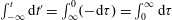 $\int _{-\infty }^{t}\text{d}t^{\prime }=\int _{\infty }^{0}(-\text{d}\unicode[STIX]{x1D70F})=\int _{0}^{\infty }\text{d}\unicode[STIX]{x1D70F}$
. The variable transformation is performed according to
$\int _{-\infty }^{t}\text{d}t^{\prime }=\int _{\infty }^{0}(-\text{d}\unicode[STIX]{x1D70F})=\int _{0}^{\infty }\text{d}\unicode[STIX]{x1D70F}$
. The variable transformation is performed according to
 $$\begin{eqnarray}\displaystyle & \displaystyle \boldsymbol{v}^{\prime }=\left(\begin{array}{@{}c@{}}v_{x}^{\prime }\\ v_{y}^{\prime }\\ v_{z}^{\prime }\end{array}\right)=\left(\begin{array}{@{}c@{}}v_{\bot }\cos (\unicode[STIX]{x1D719}+\unicode[STIX]{x1D6FA}\unicode[STIX]{x1D70F})\\ v_{\bot }\sin (\unicode[STIX]{x1D719}+\unicode[STIX]{x1D6FA}\unicode[STIX]{x1D70F})\\ v_{\Vert }\end{array}\right) & \displaystyle\end{eqnarray}$$
 $$\begin{eqnarray}\displaystyle & \displaystyle \boldsymbol{x}^{\prime }=\left(\begin{array}{@{}c@{}}x^{\prime }\\ y^{\prime }\\ z^{\prime }\end{array}\right)=\left(\begin{array}{@{}c@{}}x\\ y\\ z\end{array}\right)+\left(\begin{array}{@{}c@{}}-\frac{v_{\bot }}{\unicode[STIX]{x1D6FA}}[\sin (\unicode[STIX]{x1D719}+\unicode[STIX]{x1D6FA}\unicode[STIX]{x1D70F})-\text{sin}\unicode[STIX]{x1D719}]\\ +\frac{v_{\bot }}{\unicode[STIX]{x1D6FA}}[\cos (\unicode[STIX]{x1D719}+\unicode[STIX]{x1D6FA}\unicode[STIX]{x1D70F})-\cos \unicode[STIX]{x1D719}]\\ -v_{\Vert }\unicode[STIX]{x1D70F}\end{array}\right), & \displaystyle\end{eqnarray}$$
which at time
 $\unicode[STIX]{x1D70F}=0$
satisfies the initial condition. Now, by straightforward calculation (and by using
$\unicode[STIX]{x1D70F}=0$
satisfies the initial condition. Now, by straightforward calculation (and by using
 $\sin (a)\cos (b)-\cos (a)\sin (b)=\sin (a-b)$
), the exponential factor is transformed as
$\sin (a)\cos (b)-\cos (a)\sin (b)=\sin (a-b)$
), the exponential factor is transformed as
 $$\begin{eqnarray}\boldsymbol{k}\boldsymbol{\cdot }\boldsymbol{x}^{\prime }-\unicode[STIX]{x1D714}t^{\prime }=\boldsymbol{k}\boldsymbol{\cdot }\boldsymbol{x}-\unicode[STIX]{x1D714}t-\frac{k_{\bot }v_{\bot }}{\unicode[STIX]{x1D6FA}}[\sin (\unicode[STIX]{x1D719}-\unicode[STIX]{x1D713}+\unicode[STIX]{x1D6FA}\unicode[STIX]{x1D70F})-\text{sin}(\unicode[STIX]{x1D719}-\unicode[STIX]{x1D713})]+(\unicode[STIX]{x1D714}-k_{\Vert }v_{\Vert })\unicode[STIX]{x1D70F},\end{eqnarray}$$
so that
 $$\begin{eqnarray}\displaystyle e^{i\boldsymbol{k}\boldsymbol{\cdot }\boldsymbol{x}^{\prime }-i\unicode[STIX]{x1D714}t^{\prime }}=e^{i\boldsymbol{k}\boldsymbol{\cdot }\boldsymbol{x}-i\unicode[STIX]{x1D714}t}e^{-i(k_{\bot }v_{\bot }/\unicode[STIX]{x1D6FA})\sin (\unicode[STIX]{x1D719}-\unicode[STIX]{x1D713}+\unicode[STIX]{x1D6FA}\unicode[STIX]{x1D70F})}e^{+i(k_{\bot }v_{\bot }/\unicode[STIX]{x1D6FA})\sin (\unicode[STIX]{x1D719}-\unicode[STIX]{x1D713})}e^{i(\unicode[STIX]{x1D714}-k_{\Vert }v_{\Vert })\unicode[STIX]{x1D70F}}. & & \displaystyle\end{eqnarray}$$
The complicated expressions encountered in the kinetic dispersion relations originate in using identity
 $$\begin{eqnarray}e^{iz\sin \unicode[STIX]{x1D719}}=\mathop{\sum }_{n=-\infty }^{\infty }e^{in\unicode[STIX]{x1D719}}\text{J}_{n}(z).\end{eqnarray}$$
There are two such exponents, and therefore the linear kinetic theory contains two independent summations, usually one through ‘
 $n$
’ and one through ‘
$n$
’ and one through ‘
 $m$
’ (which should not be confused with mass), i.e.
$m$
’ (which should not be confused with mass), i.e.
 $$\begin{eqnarray}\displaystyle & \displaystyle e^{-i(k_{\bot }v_{\bot }/\unicode[STIX]{x1D6FA})\sin (\unicode[STIX]{x1D719}-\unicode[STIX]{x1D713}+\unicode[STIX]{x1D6FA}\unicode[STIX]{x1D70F})}=\mathop{\sum }_{n=-\infty }^{\infty }e^{-in(\unicode[STIX]{x1D719}-\unicode[STIX]{x1D713}+\unicode[STIX]{x1D6FA}\unicode[STIX]{x1D70F})}\text{J}_{n}\left(\frac{k_{\bot }v_{\bot }}{\unicode[STIX]{x1D6FA}}\right); & \displaystyle\end{eqnarray}$$
 $$\begin{eqnarray}\displaystyle & \displaystyle e^{+i(k_{\bot }v_{\bot }/\unicode[STIX]{x1D6FA})\sin (\unicode[STIX]{x1D719}-\unicode[STIX]{x1D713})}=\mathop{\sum }_{m=-\infty }^{\infty }e^{+im(\unicode[STIX]{x1D719}-\unicode[STIX]{x1D713})}\text{J}_{m}\left(\frac{k_{\bot }v_{\bot }}{\unicode[STIX]{x1D6FA}}\right), & \displaystyle\end{eqnarray}$$
and together
 $$\begin{eqnarray}\displaystyle & & \displaystyle e^{-i(k_{\bot }v_{\bot }/\unicode[STIX]{x1D6FA})\sin (\unicode[STIX]{x1D719}-\unicode[STIX]{x1D713}+\unicode[STIX]{x1D6FA}\unicode[STIX]{x1D70F})}e^{+i(k_{\bot }v_{\bot }/\unicode[STIX]{x1D6FA})\sin (\unicode[STIX]{x1D719}-\unicode[STIX]{x1D713})}\nonumber\\ \displaystyle & & \displaystyle \qquad =\mathop{\sum }_{n=-\infty }^{\infty }\mathop{\sum }_{m=-\infty }^{\infty }e^{+i(m-n)(\unicode[STIX]{x1D719}-\unicode[STIX]{x1D713})}e^{-in\unicode[STIX]{x1D6FA}\unicode[STIX]{x1D70F}}\text{J}_{n}\left(\frac{k_{\bot }v_{\bot }}{\unicode[STIX]{x1D6FA}}\right)\text{J}_{m}\left(\frac{k_{\bot }v_{\bot }}{\unicode[STIX]{x1D6FA}}\right).\end{eqnarray}$$
It is obvious that the quantity
 $k_{\bot }v_{\bot }/\unicode[STIX]{x1D6FA}$
will be always present and it is useful to use some abbreviations. Each book chooses a different notation, Swanson uses ‘b’, Stix uses ‘z’, etc. Since we are interested in Landau fluid models, we choose to follow the notation of Passot and Sulem 2006 and call this quantity for
$k_{\bot }v_{\bot }/\unicode[STIX]{x1D6FA}$
will be always present and it is useful to use some abbreviations. Each book chooses a different notation, Swanson uses ‘b’, Stix uses ‘z’, etc. Since we are interested in Landau fluid models, we choose to follow the notation of Passot and Sulem 2006 and call this quantity for
 $r$
-species
$r$
-species
 $\unicode[STIX]{x1D706}_{r}$
, soFootnote
12
$\unicode[STIX]{x1D706}_{r}$
, soFootnote
12
 $$\begin{eqnarray}\unicode[STIX]{x1D706}_{r}\equiv \frac{k_{\bot }v_{\bot }}{\unicode[STIX]{x1D6FA}_{r}},\end{eqnarray}$$
where for clarity of calculations, we again drop the species index
 $r$
. The transformation of the full exponential factor (C 8) therefore yields
$r$
. The transformation of the full exponential factor (C 8) therefore yields
 $$\begin{eqnarray}\displaystyle e^{i\boldsymbol{k}\boldsymbol{\cdot }\boldsymbol{x}^{\prime }-i\unicode[STIX]{x1D714}t^{\prime }}=e^{i\boldsymbol{k}\boldsymbol{\cdot }\boldsymbol{x}-i\unicode[STIX]{x1D714}t}\mathop{\sum }_{n=-\infty }^{\infty }\mathop{\sum }_{m=-\infty }^{\infty }e^{+i(m-n)(\unicode[STIX]{x1D719}-\unicode[STIX]{x1D713})}e^{+i(\unicode[STIX]{x1D714}-k_{\Vert }v_{\Vert }-n\unicode[STIX]{x1D6FA})\unicode[STIX]{x1D70F}}\text{J}_{n}(\unicode[STIX]{x1D706})\text{J}_{m}(\unicode[STIX]{x1D706}). & & \displaystyle\end{eqnarray}$$
Using this result in (C 2) allows the usual cancellation of the exponential factor
 $e^{i\boldsymbol{k}\boldsymbol{\cdot }\boldsymbol{x}-i\unicode[STIX]{x1D714}t}$
on both sides of the Fourier transformed equation, a step that we omitted to explicitly write down many times before. The partially transformed equation (C 2) therefore reads
$e^{i\boldsymbol{k}\boldsymbol{\cdot }\boldsymbol{x}-i\unicode[STIX]{x1D714}t}$
on both sides of the Fourier transformed equation, a step that we omitted to explicitly write down many times before. The partially transformed equation (C 2) therefore reads
 $$\begin{eqnarray}\displaystyle f^{(1)} & = & \displaystyle -\frac{q_{r}}{m_{r}}\int _{0}^{\infty }\left[\mathop{\sum }_{n=-\infty }^{\infty }\mathop{\sum }_{m=-\infty }^{\infty }e^{+i(m-n)(\unicode[STIX]{x1D719}-\unicode[STIX]{x1D713})}e^{+i(\unicode[STIX]{x1D714}-k_{\Vert }v_{\Vert }-n\unicode[STIX]{x1D6FA})\unicode[STIX]{x1D70F}}\right.\nonumber\\ \displaystyle & & \displaystyle \left.\times \,\text{J}_{n}(\unicode[STIX]{x1D706})\text{J}_{m}(\unicode[STIX]{x1D706})\left(\boldsymbol{E}^{(1)}+\frac{1}{c}\boldsymbol{v}^{\prime }\times \boldsymbol{B}^{(1)}\right)\boldsymbol{\cdot }\unicode[STIX]{x1D735}_{v^{\prime }}f_{0}(\boldsymbol{v}^{\prime })\right]\,\text{d}\unicode[STIX]{x1D70F},\end{eqnarray}$$
where we still did not perform the coordinate change in the operator at the end of the equation. From now on, for the electric and magnetic fields we drop the superscript (1). Let us first calculate the gradient
 $\unicode[STIX]{x1D735}_{v^{\prime }}f_{0}(\boldsymbol{v}^{\prime })$
.
$\unicode[STIX]{x1D735}_{v^{\prime }}f_{0}(\boldsymbol{v}^{\prime })$
.
It is useful to emphasize a very important property
 $$\begin{eqnarray}|\boldsymbol{v}_{\bot }^{\prime }|^{2}=v_{x}^{\prime 2}+v_{y}^{\prime 2}=v_{\bot }^{2}\cos ^{2}(\unicode[STIX]{x1D719}+\unicode[STIX]{x1D6FA}\unicode[STIX]{x1D70F})+v_{\bot }^{2}\sin ^{2}(\unicode[STIX]{x1D719}+\unicode[STIX]{x1D6FA}\unicode[STIX]{x1D70F})=|\boldsymbol{v}_{\bot }|^{2},\end{eqnarray}$$
or in another words
 $|\boldsymbol{v}_{\bot }^{\prime }|=|\boldsymbol{v}_{\bot }|$
that is often abbreviated with non-bolded
$|\boldsymbol{v}_{\bot }^{\prime }|=|\boldsymbol{v}_{\bot }|$
that is often abbreviated with non-bolded
 $v_{\bot }^{\prime }=v_{\bot }$
(and since
$v_{\bot }^{\prime }=v_{\bot }$
(and since
 $v_{\Vert }^{\prime }=v_{\Vert }$
also
$v_{\Vert }^{\prime }=v_{\Vert }$
also
 $|\boldsymbol{v}^{\prime }|=|\boldsymbol{v}|$
). At first, it can be perhaps a bit confusing when one writes that the non-bolded
$|\boldsymbol{v}^{\prime }|=|\boldsymbol{v}|$
). At first, it can be perhaps a bit confusing when one writes that the non-bolded
 $v_{\bot }^{\prime }=v_{\bot }$
, since
$v_{\bot }^{\prime }=v_{\bot }$
, since
 $v_{x}^{\prime }\neq v_{x}$
,
$v_{x}^{\prime }\neq v_{x}$
,
 $v_{y}^{\prime }\neq v_{y}$
and also the bolded
$v_{y}^{\prime }\neq v_{y}$
and also the bolded
 $\boldsymbol{v}^{\prime }\neq \boldsymbol{v}$
. The above identity implies that for the gyrotropic
$\boldsymbol{v}^{\prime }\neq \boldsymbol{v}$
. The above identity implies that for the gyrotropic
 $f_{0}$
(which is a strict requirement for
$f_{0}$
(which is a strict requirement for
 $f_{0}$
)
$f_{0}$
)
 $$\begin{eqnarray}f_{0}(|\boldsymbol{v}_{\bot }^{\prime }|^{2},v_{\Vert }^{\prime })=f_{0}(|\boldsymbol{v}_{\bot }|^{2},v_{\Vert }),\end{eqnarray}$$
further implying that
 $$\begin{eqnarray}\frac{\unicode[STIX]{x2202}f_{0}}{\unicode[STIX]{x2202}v_{\bot }^{\prime }}\equiv \frac{\unicode[STIX]{x2202}f_{0}}{\unicode[STIX]{x2202}|\boldsymbol{v}_{\bot }^{\prime }|}=\frac{\unicode[STIX]{x2202}f_{0}}{\unicode[STIX]{x2202}|\boldsymbol{v}_{\bot }|}\equiv \frac{\unicode[STIX]{x2202}f_{0}}{\unicode[STIX]{x2202}v_{\bot }}.\end{eqnarray}$$
The
 $\unicode[STIX]{x1D735}_{v^{\prime }}f_{0}$
can now be calculated easily, since
$\unicode[STIX]{x1D735}_{v^{\prime }}f_{0}$
can now be calculated easily, since
 $$\begin{eqnarray}\displaystyle \frac{\unicode[STIX]{x2202}f_{0}}{\unicode[STIX]{x2202}v_{x}^{\prime }}=\frac{\unicode[STIX]{x2202}f_{0}}{\unicode[STIX]{x2202}|\boldsymbol{v}_{\bot }^{\prime }|}\frac{\unicode[STIX]{x2202}|\boldsymbol{v}_{\bot }^{\prime }|}{\unicode[STIX]{x2202}v_{x}^{\prime }}=\frac{\unicode[STIX]{x2202}f_{0}}{\unicode[STIX]{x2202}v_{\bot }}\frac{v_{x}^{\prime }}{v_{\bot }};\quad \frac{\unicode[STIX]{x2202}f_{0}}{\unicode[STIX]{x2202}v_{y}^{\prime }}=\frac{\unicode[STIX]{x2202}f_{0}}{\unicode[STIX]{x2202}v_{\bot }}\frac{v_{y}^{\prime }}{v_{\bot }}, & & \displaystyle\end{eqnarray}$$
and the gradient is written as (for gyrotropic
 $\unicode[STIX]{x2202}f_{0}/\unicode[STIX]{x2202}\unicode[STIX]{x1D719}=0$
)
$\unicode[STIX]{x2202}f_{0}/\unicode[STIX]{x2202}\unicode[STIX]{x1D719}=0$
)
 $$\begin{eqnarray}\displaystyle \unicode[STIX]{x1D735}_{v^{\prime }}f_{0}=\left(\begin{array}{@{}c@{}}\frac{v_{x}^{\prime }}{v_{\bot }}\frac{\unicode[STIX]{x2202}}{\unicode[STIX]{x2202}v_{\bot }}\\ \frac{v_{y}^{\prime }}{v_{\bot }}\frac{\unicode[STIX]{x2202}}{\unicode[STIX]{x2202}v_{\bot }}\\ \frac{\unicode[STIX]{x2202}}{\unicode[STIX]{x2202}v_{\Vert }}\end{array}\right)\quad f_{0}=\left(\begin{array}{@{}c@{}}\cos (\unicode[STIX]{x1D719}+\unicode[STIX]{x1D6FA}\unicode[STIX]{x1D70F})\frac{\unicode[STIX]{x2202}}{\unicode[STIX]{x2202}v_{\bot }}\\ \sin (\unicode[STIX]{x1D719}+\unicode[STIX]{x1D6FA}\unicode[STIX]{x1D70F})\frac{\unicode[STIX]{x2202}}{\unicode[STIX]{x2202}v_{\bot }}\\ \frac{\unicode[STIX]{x2202}}{\unicode[STIX]{x2202}v_{\Vert }}\end{array}\right)f_{0}. & & \displaystyle\end{eqnarray}$$
It is actually simpler to postpone the introduction of angles
 $\unicode[STIX]{x1D719},\unicode[STIX]{x1D713}$
and for a moment keep a general notation
$\unicode[STIX]{x1D719},\unicode[STIX]{x1D713}$
and for a moment keep a general notation
 $\boldsymbol{v}^{\prime }=(v_{x}^{\prime },v_{y}^{\prime },v_{z}^{\prime })$
and
$\boldsymbol{v}^{\prime }=(v_{x}^{\prime },v_{y}^{\prime },v_{z}^{\prime })$
and
 $\boldsymbol{k}=(k_{x},k_{y},k_{z})$
. To transform the
$\boldsymbol{k}=(k_{x},k_{y},k_{z})$
. To transform the
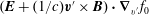 $(\boldsymbol{E}+(1/c)\boldsymbol{v}^{\prime }\times \boldsymbol{B})\boldsymbol{\cdot }\unicode[STIX]{x1D735}_{v^{\prime }}f_{0}$
, one can do the completely same operations as were done in the previous subsection where the operator
$(\boldsymbol{E}+(1/c)\boldsymbol{v}^{\prime }\times \boldsymbol{B})\boldsymbol{\cdot }\unicode[STIX]{x1D735}_{v^{\prime }}f_{0}$
, one can do the completely same operations as were done in the previous subsection where the operator
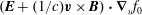 $(\boldsymbol{E}+(1/c)\boldsymbol{v}\times \boldsymbol{B})\boldsymbol{\cdot }\unicode[STIX]{x1D735}_{v}f_{0}$
was considered. One can just use the result (B 9), add primes to all velocities and delete those on
$(\boldsymbol{E}+(1/c)\boldsymbol{v}\times \boldsymbol{B})\boldsymbol{\cdot }\unicode[STIX]{x1D735}_{v}f_{0}$
was considered. One can just use the result (B 9), add primes to all velocities and delete those on
 $v_{\bot }^{\prime }=v_{\bot }$
,
$v_{\bot }^{\prime }=v_{\bot }$
,
 $v_{\Vert }^{\prime }=v_{\Vert }$
, finally yielding
$v_{\Vert }^{\prime }=v_{\Vert }$
, finally yielding
 $$\begin{eqnarray}\displaystyle \left(\boldsymbol{E}+\frac{1}{c}\boldsymbol{v}^{\prime }\times \boldsymbol{B}\right)\boldsymbol{\cdot }\unicode[STIX]{x1D735}_{v^{\prime }}f_{0} & = & \displaystyle (E_{x}v_{x}^{\prime }+E_{y}v_{y}^{\prime })\left[\left(1-\frac{v_{\Vert }k_{\Vert }}{\unicode[STIX]{x1D714}}\right)\frac{1}{v_{\bot }}\frac{\unicode[STIX]{x2202}f_{0}}{\unicode[STIX]{x2202}v_{\bot }}+\frac{k_{\Vert }}{\unicode[STIX]{x1D714}}\frac{\unicode[STIX]{x2202}f_{0}}{\unicode[STIX]{x2202}v_{\Vert }}\right]\nonumber\\ \displaystyle & & \displaystyle +\,E_{z}\left[\frac{\unicode[STIX]{x2202}f_{0}}{\unicode[STIX]{x2202}v_{\Vert }}-\frac{v_{x}^{\prime }k_{x}+v_{y}^{\prime }k_{y}}{\unicode[STIX]{x1D714}}\left(\frac{\unicode[STIX]{x2202}f_{0}}{\unicode[STIX]{x2202}v_{\Vert }}-\frac{v_{\Vert }}{v_{\bot }}\frac{\unicode[STIX]{x2202}f_{0}}{\unicode[STIX]{x2202}v_{\bot }}\right)\right],\end{eqnarray}$$
which is equivalent to equation (4.83) in Swanson. Only now we introduce the angles and finish the transformation. Since
 $$\begin{eqnarray}\displaystyle v_{x}^{\prime }k_{x}+v_{y}^{\prime }k_{y} & = & \displaystyle v_{\bot }\cos (\unicode[STIX]{x1D719}+\unicode[STIX]{x1D6FA}\unicode[STIX]{x1D70F})k_{\bot }\cos \unicode[STIX]{x1D713}+v_{\bot }\sin (\unicode[STIX]{x1D719}+\unicode[STIX]{x1D6FA}\unicode[STIX]{x1D70F})k_{\bot }\sin \unicode[STIX]{x1D713}\nonumber\\ \displaystyle & = & \displaystyle v_{\bot }k_{\bot }\cos (\unicode[STIX]{x1D719}+\unicode[STIX]{x1D6FA}\unicode[STIX]{x1D70F}-\unicode[STIX]{x1D713}),\end{eqnarray}$$
the transformation yields
 $$\begin{eqnarray}\displaystyle & & \displaystyle \left(\boldsymbol{E}+\frac{1}{c}\boldsymbol{v}^{\prime }\times \boldsymbol{B}\right)\boldsymbol{\cdot }\unicode[STIX]{x1D735}_{v^{\prime }}f_{0}\nonumber\\ \displaystyle & & \displaystyle \quad =\left(E_{x}\cos (\unicode[STIX]{x1D719}+\unicode[STIX]{x1D6FA}\unicode[STIX]{x1D70F})+E_{y}\sin (\unicode[STIX]{x1D719}+\unicode[STIX]{x1D6FA}\unicode[STIX]{x1D70F})\right)\left[\left(1-\frac{v_{\Vert }k_{\Vert }}{\unicode[STIX]{x1D714}}\right)\frac{\unicode[STIX]{x2202}f_{0}}{\unicode[STIX]{x2202}v_{\bot }}+\frac{k_{\Vert }v_{\bot }}{\unicode[STIX]{x1D714}}\frac{\unicode[STIX]{x2202}f_{0}}{\unicode[STIX]{x2202}v_{\Vert }}\right]\nonumber\\ \displaystyle & & \displaystyle \qquad +\,E_{z}\left[\frac{\unicode[STIX]{x2202}f_{0}}{\unicode[STIX]{x2202}v_{\Vert }}+\frac{k_{\bot }}{\unicode[STIX]{x1D714}}\cos (\unicode[STIX]{x1D719}+\unicode[STIX]{x1D6FA}\unicode[STIX]{x1D70F}-\unicode[STIX]{x1D713})\left(v_{\Vert }\frac{\unicode[STIX]{x2202}f_{0}}{\unicode[STIX]{x2202}v_{\bot }}-v_{\bot }\frac{\unicode[STIX]{x2202}f_{0}}{\unicode[STIX]{x2202}v_{\Vert }}\right)\right].\end{eqnarray}$$
To be clear, let us write down the complete result (C 15) that we have for now
 $$\begin{eqnarray}\displaystyle f^{(1)} & = & \displaystyle -\frac{q_{r}}{m_{r}}\int _{0}^{\infty }\mathop{\sum }_{n=-\infty }^{\infty }\mathop{\sum }_{m=-\infty }^{\infty }e^{+i(m-n)(\unicode[STIX]{x1D719}-\unicode[STIX]{x1D713})}e^{+i(\unicode[STIX]{x1D714}-k_{\Vert }v_{\Vert }-n\unicode[STIX]{x1D6FA})\unicode[STIX]{x1D70F}}\text{J}_{n}(\unicode[STIX]{x1D706})\text{J}_{m}(\unicode[STIX]{x1D706})\nonumber\\ \displaystyle & & \displaystyle \times \,\left\{\left(E_{x}\cos (\unicode[STIX]{x1D719}+\unicode[STIX]{x1D6FA}\unicode[STIX]{x1D70F})+E_{y}\sin (\unicode[STIX]{x1D719}+\unicode[STIX]{x1D6FA}\unicode[STIX]{x1D70F})\right)\left[\left(1-\frac{v_{\Vert }k_{\Vert }}{\unicode[STIX]{x1D714}}\right)\frac{\unicode[STIX]{x2202}f_{0}}{\unicode[STIX]{x2202}v_{\bot }}+\frac{k_{\Vert }v_{\bot }}{\unicode[STIX]{x1D714}}\frac{\unicode[STIX]{x2202}f_{0}}{\unicode[STIX]{x2202}v_{\Vert }}\right]\right.\nonumber\\ \displaystyle & & \displaystyle \left.+\,E_{z}\left[\frac{\unicode[STIX]{x2202}f_{0}}{\unicode[STIX]{x2202}v_{\Vert }}+\frac{k_{\bot }}{\unicode[STIX]{x1D714}}\left(v_{\Vert }\frac{\unicode[STIX]{x2202}f_{0}}{\unicode[STIX]{x2202}v_{\bot }}-v_{\bot }\frac{\unicode[STIX]{x2202}f_{0}}{\unicode[STIX]{x2202}v_{\Vert }}\right)\cos (\unicode[STIX]{x1D719}+\unicode[STIX]{x1D6FA}\unicode[STIX]{x1D70F}-\unicode[STIX]{x1D713})\right]\right\}\,\text{d}\unicode[STIX]{x1D70F},\end{eqnarray}$$
where the
 $\times$
at the beginning of the second line is just a multiplication and not a cross-product (the equation is not written in the vector form anyway). The result agrees with Stix’s expressions (10.38) and (10.39), even though Stix at this stage did not use the Bessel expansion yet. Stix now does not proceed with the evaluation of the integral along
$\times$
at the beginning of the second line is just a multiplication and not a cross-product (the equation is not written in the vector form anyway). The result agrees with Stix’s expressions (10.38) and (10.39), even though Stix at this stage did not use the Bessel expansion yet. Stix now does not proceed with the evaluation of the integral along
 $\unicode[STIX]{x1D70F}$
, and instead goes ahead and already starts to partially calculate the first-order velocity moment with integrals
$\unicode[STIX]{x1D70F}$
, and instead goes ahead and already starts to partially calculate the first-order velocity moment with integrals
 $\int \boldsymbol{v}f^{(1)}\,\text{d}^{3}v$
(first integrating over
$\int \boldsymbol{v}f^{(1)}\,\text{d}^{3}v$
(first integrating over
 $\int _{0}^{2\unicode[STIX]{x03C0}}\,\text{d}\unicode[STIX]{x1D719}$
) to eventually obtain the kinetic current
$\int _{0}^{2\unicode[STIX]{x03C0}}\,\text{d}\unicode[STIX]{x1D719}$
) to eventually obtain the kinetic current
 $\boldsymbol{j}=\sum _{r}q_{r}n_{r}\boldsymbol{u}_{r}=\sum _{r}q_{r}\int \boldsymbol{v}_{r}f_{r}^{(1)}\,\text{d}^{3}v_{r}$
and the conductivity matrix
$\boldsymbol{j}=\sum _{r}q_{r}n_{r}\boldsymbol{u}_{r}=\sum _{r}q_{r}\int \boldsymbol{v}_{r}f_{r}^{(1)}\,\text{d}^{3}v_{r}$
and the conductivity matrix
 $(\unicode[STIX]{x1D748})_{ij}$
(through
$(\unicode[STIX]{x1D748})_{ij}$
(through
 $\boldsymbol{j}=\unicode[STIX]{x1D748}\boldsymbol{\cdot }\boldsymbol{E}$
) that leads to the kinetic dispersion relation. Stix actually first derives (C 23) plugged into (C 2). After introducing the Bessel expansion, Stix immediately performs the integration over
$\boldsymbol{j}=\unicode[STIX]{x1D748}\boldsymbol{\cdot }\boldsymbol{E}$
) that leads to the kinetic dispersion relation. Stix actually first derives (C 23) plugged into (C 2). After introducing the Bessel expansion, Stix immediately performs the integration over
 $\text{d}\unicode[STIX]{x1D719}$
. The integration over
$\text{d}\unicode[STIX]{x1D719}$
. The integration over
 $\unicode[STIX]{x1D70F}$
is done later during other calculations, and this somewhat simplifies the amount of algebra that needs to be written down. The simplified algebra is beneficial and surely appreciated by experienced kinetic researchers, however, especially for new researchers, it somewhat blurs the main point, how the kinetic dispersion relation is derived. The kinetic dispersion relation is derived by obtaining the
$\unicode[STIX]{x1D70F}$
is done later during other calculations, and this somewhat simplifies the amount of algebra that needs to be written down. The simplified algebra is beneficial and surely appreciated by experienced kinetic researchers, however, especially for new researchers, it somewhat blurs the main point, how the kinetic dispersion relation is derived. The kinetic dispersion relation is derived by obtaining the
 $f^{(1)}$
, and by calculating the current
$f^{(1)}$
, and by calculating the current
 $\boldsymbol{j}$
. Moreover, we later want to obtain higher-order moments of
$\boldsymbol{j}$
. Moreover, we later want to obtain higher-order moments of
 $f^{(1)}$
than just the first-order velocity moment. We therefore follow Swanson, Akheizer, Passot and Sulem, and finish the calculation of
$f^{(1)}$
than just the first-order velocity moment. We therefore follow Swanson, Akheizer, Passot and Sulem, and finish the calculation of
 $f^{(1)}$
by evaluating the
$f^{(1)}$
by evaluating the
 $\int _{0}^{\infty }\text{d}\unicode[STIX]{x1D70F}$
integral in (C 24).
$\int _{0}^{\infty }\text{d}\unicode[STIX]{x1D70F}$
integral in (C 24).
By examining equation (C 24), there is only one factor that is
 $\unicode[STIX]{x1D70F}$
dependent in the first line that needs to be integrated,
$\unicode[STIX]{x1D70F}$
dependent in the first line that needs to be integrated,
 $e^{i(\unicode[STIX]{x1D714}-k_{\Vert }v_{\Vert }-n\unicode[STIX]{x1D6FA})\unicode[STIX]{x1D70F}}$
, and the factor is multiplied by four different possibilities,
$e^{i(\unicode[STIX]{x1D714}-k_{\Vert }v_{\Vert }-n\unicode[STIX]{x1D6FA})\unicode[STIX]{x1D70F}}$
, and the factor is multiplied by four different possibilities,
 $\cos (\unicode[STIX]{x1D719}+\unicode[STIX]{x1D6FA}\unicode[STIX]{x1D70F})$
,
$\cos (\unicode[STIX]{x1D719}+\unicode[STIX]{x1D6FA}\unicode[STIX]{x1D70F})$
,
 $\sin (\unicode[STIX]{x1D719}+\unicode[STIX]{x1D6FA}\unicode[STIX]{x1D70F})$
, 1 and
$\sin (\unicode[STIX]{x1D719}+\unicode[STIX]{x1D6FA}\unicode[STIX]{x1D70F})$
, 1 and
 $\cos (\unicode[STIX]{x1D719}+\unicode[STIX]{x1D6FA}\unicode[STIX]{x1D70F}-\unicode[STIX]{x1D713})$
. We first need to examine the following integral
$\cos (\unicode[STIX]{x1D719}+\unicode[STIX]{x1D6FA}\unicode[STIX]{x1D70F}-\unicode[STIX]{x1D713})$
. We first need to examine the following integral
 $$\begin{eqnarray}\int _{0}^{\infty }e^{iax}\,\text{d}x=\frac{i}{a};\quad \text{if }\text{Im}(a)>0.\end{eqnarray}$$
This perhaps surprising integral can be easily verified since an indefinite integral
 $e^{iax}/(ia)$
exists and the curious limit
$e^{iax}/(ia)$
exists and the curious limit
 $$\begin{eqnarray}\lim _{x\rightarrow \infty }e^{iax}=\lim _{x\rightarrow \infty }e^{i[\text{Re}(a)+i\text{Im}(a)]x}=\lim _{x\rightarrow \infty }e^{i\text{Re}(a)x}e^{-\text{Im}(a)x}=0;\quad \text{if }\text{Im}(a)>0.\end{eqnarray}$$
Obviously, the
 $\text{Im}(a)>0$
is a strict requirement. If
$\text{Im}(a)>0$
is a strict requirement. If
 $\text{Im}(a)=0$
, the limit is undefined since
$\text{Im}(a)=0$
, the limit is undefined since
 $\cos (x)$
and
$\cos (x)$
and
 $\sin (x)$
always oscillate, and if
$\sin (x)$
always oscillate, and if
 $\text{Im}(a)<0$
the limit diverges to
$\text{Im}(a)<0$
the limit diverges to
 $\pm \infty$
. Therefore, one of the four needed integrals is
$\pm \infty$
. Therefore, one of the four needed integrals is
 $$\begin{eqnarray}\int _{0}^{\infty }e^{i(\unicode[STIX]{x1D714}-k_{\Vert }v_{\Vert }-n\unicode[STIX]{x1D6FA})\unicode[STIX]{x1D70F}}\,\text{d}\unicode[STIX]{x1D70F}=\frac{i}{\unicode[STIX]{x1D714}-k_{\Vert }v_{\Vert }-n\unicode[STIX]{x1D6FA}};\quad \text{if }\text{Im}(\unicode[STIX]{x1D714})>0,\end{eqnarray}$$
where the
 $\text{Im}(\unicode[STIX]{x1D714})>0$
requirement is obtained, because
$\text{Im}(\unicode[STIX]{x1D714})>0$
requirement is obtained, because
 $k_{\Vert }$
,
$k_{\Vert }$
,
 $v_{\Vert }$
,
$v_{\Vert }$
,
 $\unicode[STIX]{x1D6FA}$
are real numbers,
$\unicode[STIX]{x1D6FA}$
are real numbers,
 $n$
is an integer and none of these can have an imaginary part. For the other 3 integrals we need
$n$
is an integer and none of these can have an imaginary part. For the other 3 integrals we need
 $$\begin{eqnarray}\displaystyle \int _{0}^{\infty }e^{ia\unicode[STIX]{x1D70F}}\cos (\unicode[STIX]{x1D719}+\unicode[STIX]{x1D6FA}\unicode[STIX]{x1D70F})\,\text{d}\unicode[STIX]{x1D70F} & = & \displaystyle \frac{1}{2}\int _{0}^{\infty }e^{ia\unicode[STIX]{x1D70F}}\left(e^{i(\unicode[STIX]{x1D719}+\unicode[STIX]{x1D6FA}\unicode[STIX]{x1D70F})}+e^{-i(\unicode[STIX]{x1D719}+\unicode[STIX]{x1D6FA}\unicode[STIX]{x1D70F})}\right)\,\text{d}\unicode[STIX]{x1D70F}\nonumber\\ \displaystyle & = & \displaystyle \frac{e^{i\unicode[STIX]{x1D719}}}{2}\int _{0}^{\infty }e^{i(a+\unicode[STIX]{x1D6FA})\unicode[STIX]{x1D70F}}\,\text{d}\unicode[STIX]{x1D70F}+\frac{e^{-i\unicode[STIX]{x1D719}}}{2}\int _{0}^{\infty }e^{i(a-\unicode[STIX]{x1D6FA})\unicode[STIX]{x1D70F}}\,\text{d}\unicode[STIX]{x1D70F}\nonumber\\ \displaystyle & = & \displaystyle \frac{e^{i\unicode[STIX]{x1D719}}}{2}\frac{i}{a+\unicode[STIX]{x1D6FA}}+\frac{e^{-i\unicode[STIX]{x1D719}}}{2}\frac{i}{a-\unicode[STIX]{x1D6FA}}\nonumber\\ \displaystyle & = & \displaystyle \frac{i}{2}\left(\frac{e^{i\unicode[STIX]{x1D719}}}{a+\unicode[STIX]{x1D6FA}}+\frac{e^{-i\unicode[STIX]{x1D719}}}{a-\unicode[STIX]{x1D6FA}}\right);\quad \text{if }\text{Im}(a)>0,\end{eqnarray}$$
and similarly
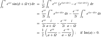 $$\begin{eqnarray}\displaystyle \int _{0}^{\infty }e^{ia\unicode[STIX]{x1D70F}}\sin (\unicode[STIX]{x1D719}+\unicode[STIX]{x1D6FA}\unicode[STIX]{x1D70F})\,\text{d}\unicode[STIX]{x1D70F} & = & \displaystyle \frac{1}{2i}\int _{0}^{\infty }e^{ia\unicode[STIX]{x1D70F}}\left(e^{i(\unicode[STIX]{x1D719}+\unicode[STIX]{x1D6FA}\unicode[STIX]{x1D70F})}-e^{-i(\unicode[STIX]{x1D719}+\unicode[STIX]{x1D6FA}\unicode[STIX]{x1D70F})}\right)\,\text{d}\unicode[STIX]{x1D70F}\nonumber\\ \displaystyle & = & \displaystyle \frac{e^{i\unicode[STIX]{x1D719}}}{2i}\int _{0}^{\infty }e^{i(a+\unicode[STIX]{x1D6FA})\unicode[STIX]{x1D70F}}\,\text{d}\unicode[STIX]{x1D70F}-\frac{e^{-i\unicode[STIX]{x1D719}}}{2i}\int _{0}^{\infty }e^{i(a-\unicode[STIX]{x1D6FA})\unicode[STIX]{x1D70F}}\,\text{d}\unicode[STIX]{x1D70F}\nonumber\\ \displaystyle & = & \displaystyle \frac{e^{i\unicode[STIX]{x1D719}}}{2i}\frac{i}{a+\unicode[STIX]{x1D6FA}}-\frac{e^{-i\unicode[STIX]{x1D719}}}{2i}\frac{i}{a-\unicode[STIX]{x1D6FA}}\nonumber\\ \displaystyle & = & \displaystyle \frac{1}{2}\left(\frac{e^{i\unicode[STIX]{x1D719}}}{a+\unicode[STIX]{x1D6FA}}-\frac{e^{-i\unicode[STIX]{x1D719}}}{a-\unicode[STIX]{x1D6FA}}\right);\quad \text{if }\text{Im}(a)>0.\end{eqnarray}$$
The 3 required integrals therefore calculate as
 $$\begin{eqnarray}\displaystyle & & \displaystyle \int _{0}^{\infty }e^{i(\unicode[STIX]{x1D714}-k_{\Vert }v_{\Vert }-n\unicode[STIX]{x1D6FA})\unicode[STIX]{x1D70F}}\cos (\unicode[STIX]{x1D719}+\unicode[STIX]{x1D6FA}\unicode[STIX]{x1D70F})\,\text{d}\unicode[STIX]{x1D70F}\nonumber\\ \displaystyle & & \displaystyle \qquad =\frac{i}{2}\left(\frac{e^{i\unicode[STIX]{x1D719}}}{\unicode[STIX]{x1D714}-k_{\Vert }v_{\Vert }-(n-1)\unicode[STIX]{x1D6FA}}+\frac{e^{-i\unicode[STIX]{x1D719}}}{\unicode[STIX]{x1D714}-k_{\Vert }v_{\Vert }-(n+1)\unicode[STIX]{x1D6FA}}\right);\end{eqnarray}$$
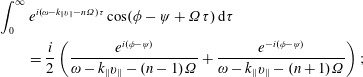 $$\begin{eqnarray}\displaystyle & & \displaystyle \int _{0}^{\infty }e^{i(\unicode[STIX]{x1D714}-k_{\Vert }v_{\Vert }-n\unicode[STIX]{x1D6FA})\unicode[STIX]{x1D70F}}\cos (\unicode[STIX]{x1D719}-\unicode[STIX]{x1D713}+\unicode[STIX]{x1D6FA}\unicode[STIX]{x1D70F})\,\text{d}\unicode[STIX]{x1D70F}\nonumber\\ \displaystyle & & \displaystyle \qquad =\frac{i}{2}\left(\frac{e^{i(\unicode[STIX]{x1D719}-\unicode[STIX]{x1D713})}}{\unicode[STIX]{x1D714}-k_{\Vert }v_{\Vert }-(n-1)\unicode[STIX]{x1D6FA}}+\frac{e^{-i(\unicode[STIX]{x1D719}-\unicode[STIX]{x1D713})}}{\unicode[STIX]{x1D714}-k_{\Vert }v_{\Vert }-(n+1)\unicode[STIX]{x1D6FA}}\right);\end{eqnarray}$$
 $$\begin{eqnarray}\displaystyle & & \displaystyle \int _{0}^{\infty }e^{i(\unicode[STIX]{x1D714}-k_{\Vert }v_{\Vert }-n\unicode[STIX]{x1D6FA})\unicode[STIX]{x1D70F}}\sin (\unicode[STIX]{x1D719}+\unicode[STIX]{x1D6FA}\unicode[STIX]{x1D70F})\,\text{d}\unicode[STIX]{x1D70F}\nonumber\\ \displaystyle & & \displaystyle \qquad =\frac{1}{2}\left(\frac{e^{i\unicode[STIX]{x1D719}}}{\unicode[STIX]{x1D714}-k_{\Vert }v_{\Vert }-(n-1)\unicode[STIX]{x1D6FA}}-\frac{e^{-i\unicode[STIX]{x1D719}}}{\unicode[STIX]{x1D714}-k_{\Vert }v_{\Vert }-(n+1)\unicode[STIX]{x1D6FA}}\right),\end{eqnarray}$$
and all 3 results require
 $\text{Im}(\unicode[STIX]{x1D714})>0$
. This strictly appearing restriction is removed later by the analytic continuation, once the fluid integrals over the
$\text{Im}(\unicode[STIX]{x1D714})>0$
. This strictly appearing restriction is removed later by the analytic continuation, once the fluid integrals over the
 $f^{(1)}$
are calculated. We therefore managed to finish the integration of (C 24) along the unperturbed orbit and our latest full result for
$f^{(1)}$
are calculated. We therefore managed to finish the integration of (C 24) along the unperturbed orbit and our latest full result for
 $f^{(1)}$
reads
$f^{(1)}$
reads
 $$\begin{eqnarray}\displaystyle & & \displaystyle f^{(1)}=-\frac{q_{r}}{m_{r}}\mathop{\sum }_{n=-\infty }^{\infty }\mathop{\sum }_{m=-\infty }^{\infty }e^{+i(m-n)(\unicode[STIX]{x1D719}-\unicode[STIX]{x1D713})}\text{J}_{n}(\unicode[STIX]{x1D706})\text{J}_{m}(\unicode[STIX]{x1D706})\nonumber\\ \displaystyle & & \displaystyle \qquad \times \,\left\{\left[\frac{iE_{x}}{2}\left(\frac{e^{i\unicode[STIX]{x1D719}}}{\unicode[STIX]{x1D714}-k_{\Vert }v_{\Vert }-(n-1)\unicode[STIX]{x1D6FA}}+\frac{e^{-i\unicode[STIX]{x1D719}}}{\unicode[STIX]{x1D714}-k_{\Vert }v_{\Vert }-(n+1)\unicode[STIX]{x1D6FA}}\right)\right.\right.\nonumber\\ \displaystyle & & \displaystyle \qquad \left.+\,\frac{E_{y}}{2}\left(\frac{e^{i\unicode[STIX]{x1D719}}}{\unicode[STIX]{x1D714}-k_{\Vert }v_{\Vert }-(n-1)\unicode[STIX]{x1D6FA}}-\frac{e^{-i\unicode[STIX]{x1D719}}}{\unicode[STIX]{x1D714}-k_{\Vert }v_{\Vert }-(n+1)\unicode[STIX]{x1D6FA}}\right)\right]\nonumber\\ \displaystyle & & \displaystyle \qquad \times \,\left[\left(1-\frac{v_{\Vert }k_{\Vert }}{\unicode[STIX]{x1D714}}\right)\frac{\unicode[STIX]{x2202}f_{0}}{\unicode[STIX]{x2202}v_{\bot }}+\frac{k_{\Vert }v_{\bot }}{\unicode[STIX]{x1D714}}\frac{\unicode[STIX]{x2202}f_{0}}{\unicode[STIX]{x2202}v_{\Vert }}\right]\nonumber\\ \displaystyle & & \displaystyle \qquad +\,E_{z}\left[\frac{i}{\unicode[STIX]{x1D714}-k_{\Vert }v_{\Vert }-n\unicode[STIX]{x1D6FA}}\frac{\unicode[STIX]{x2202}f_{0}}{\unicode[STIX]{x2202}v_{\Vert }}+\frac{k_{\bot }}{\unicode[STIX]{x1D714}}\left(v_{\Vert }\frac{\unicode[STIX]{x2202}f_{0}}{\unicode[STIX]{x2202}v_{\bot }}-v_{\bot }\frac{\unicode[STIX]{x2202}f_{0}}{\unicode[STIX]{x2202}v_{\Vert }}\right)\right.\nonumber\\ \displaystyle & & \displaystyle \qquad \left.\left.\times \,\frac{i}{2}\left(\frac{e^{i(\unicode[STIX]{x1D719}-\unicode[STIX]{x1D713})}}{\unicode[STIX]{x1D714}-k_{\Vert }v_{\Vert }-(n-1)\unicode[STIX]{x1D6FA}}+\frac{e^{-i(\unicode[STIX]{x1D719}-\unicode[STIX]{x1D713})}}{\unicode[STIX]{x1D714}-k_{\Vert }v_{\Vert }-(n+1)\unicode[STIX]{x1D6FA}}\right)\right]\right\}.\end{eqnarray}$$
Obviously, the result is not very pretty, and we would like somehow to pull out the denominator
 $\unicode[STIX]{x1D714}-k_{\Vert }v_{\Vert }-n\unicode[STIX]{x1D6FA}$
from all the expressions, so that the ‘resonances’ are grouped together. The trouble is the shifted
$\unicode[STIX]{x1D714}-k_{\Vert }v_{\Vert }-n\unicode[STIX]{x1D6FA}$
from all the expressions, so that the ‘resonances’ are grouped together. The trouble is the shifted
 $(n-1)\unicode[STIX]{x1D6FA}$
and
$(n-1)\unicode[STIX]{x1D6FA}$
and
 $(n+1)\unicode[STIX]{x1D6FA}$
. However, all expressions are preceded by
$(n+1)\unicode[STIX]{x1D6FA}$
. However, all expressions are preceded by
 $\sum _{n=-\infty }^{\infty }$
. It is therefore easy to shift the summation by one index, where terms that contain
$\sum _{n=-\infty }^{\infty }$
. It is therefore easy to shift the summation by one index, where terms that contain
 $(n-1)\unicode[STIX]{x1D6FA}$
require shift
$(n-1)\unicode[STIX]{x1D6FA}$
require shift
 $n=l+1$
, and terms that contain
$n=l+1$
, and terms that contain
 $(n+1)\unicode[STIX]{x1D6FA}$
require shift
$(n+1)\unicode[STIX]{x1D6FA}$
require shift
 $n=l-1$
. The transformation is easy to calculate, for example the terms proportional to
$n=l-1$
. The transformation is easy to calculate, for example the terms proportional to
 $E_{x}$
transform as
$E_{x}$
transform as
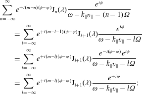 $$\begin{eqnarray}\displaystyle & & \displaystyle \mathop{\sum }_{n=-\infty }^{\infty }e^{+i(m-n)(\unicode[STIX]{x1D719}-\unicode[STIX]{x1D713})}\text{J}_{n}(\unicode[STIX]{x1D706})\frac{e^{i\unicode[STIX]{x1D719}}}{\unicode[STIX]{x1D714}-k_{\Vert }v_{\Vert }-(n-1)\unicode[STIX]{x1D6FA}}\nonumber\\ \displaystyle & & \displaystyle \qquad =\mathop{\sum }_{l=-\infty }^{\infty }e^{+i(m-l-1)(\unicode[STIX]{x1D719}-\unicode[STIX]{x1D713})}\text{J}_{l+1}(\unicode[STIX]{x1D706})\frac{e^{i\unicode[STIX]{x1D719}}}{\unicode[STIX]{x1D714}-k_{\Vert }v_{\Vert }-l\unicode[STIX]{x1D6FA}}\nonumber\\ \displaystyle & & \displaystyle \qquad =\mathop{\sum }_{l=-\infty }^{\infty }e^{+i(m-l)(\unicode[STIX]{x1D719}-\unicode[STIX]{x1D713})}\text{J}_{l+1}(\unicode[STIX]{x1D706})\frac{e^{-i(\unicode[STIX]{x1D719}-\unicode[STIX]{x1D713})}e^{i\unicode[STIX]{x1D719}}}{\unicode[STIX]{x1D714}-k_{\Vert }v_{\Vert }-l\unicode[STIX]{x1D6FA}}\nonumber\\ \displaystyle & & \displaystyle \qquad =\mathop{\sum }_{l=-\infty }^{\infty }e^{+i(m-l)(\unicode[STIX]{x1D719}-\unicode[STIX]{x1D713})}\text{J}_{l+1}(\unicode[STIX]{x1D706})\frac{e^{+i\unicode[STIX]{x1D713}}}{\unicode[STIX]{x1D714}-k_{\Vert }v_{\Vert }-l\unicode[STIX]{x1D6FA}};\end{eqnarray}$$
 $$\begin{eqnarray}\displaystyle & & \displaystyle \mathop{\sum }_{n=-\infty }^{\infty }e^{+i(m-n)(\unicode[STIX]{x1D719}-\unicode[STIX]{x1D713})}\text{J}_{n}(\unicode[STIX]{x1D706})\frac{e^{-i\unicode[STIX]{x1D719}}}{\unicode[STIX]{x1D714}-k_{\Vert }v_{\Vert }-(n+1)\unicode[STIX]{x1D6FA}}\nonumber\\ \displaystyle & & \displaystyle \qquad =\mathop{\sum }_{l=-\infty }^{\infty }e^{+i(m-l+1)(\unicode[STIX]{x1D719}-\unicode[STIX]{x1D713})}\text{J}_{l-1}(\unicode[STIX]{x1D706})\frac{e^{-i\unicode[STIX]{x1D719}}}{\unicode[STIX]{x1D714}-k_{\Vert }v_{\Vert }-l\unicode[STIX]{x1D6FA}}\nonumber\\ \displaystyle & & \displaystyle \qquad =\mathop{\sum }_{l=-\infty }^{\infty }e^{+i(m-l)(\unicode[STIX]{x1D719}-\unicode[STIX]{x1D713})}\text{J}_{l-1}(\unicode[STIX]{x1D706})\frac{e^{-i\unicode[STIX]{x1D713}}}{\unicode[STIX]{x1D714}-k_{\Vert }v_{\Vert }-l\unicode[STIX]{x1D6FA}}.\end{eqnarray}$$
Adding the two equations together, both
 $E_{x}$
terms therefore transform as
$E_{x}$
terms therefore transform as
 $$\begin{eqnarray}\displaystyle (\text{C}\,34)+(\text{C}\,35)=\mathop{\sum }_{l=-\infty }^{\infty }\frac{e^{+i(m-l)(\unicode[STIX]{x1D719}-\unicode[STIX]{x1D713})}}{\unicode[STIX]{x1D714}-k_{\Vert }v_{\Vert }-l\unicode[STIX]{x1D6FA}}\left(\text{J}_{l+1}(\unicode[STIX]{x1D706})e^{+i\unicode[STIX]{x1D713}}+\text{J}_{l-1}(\unicode[STIX]{x1D706})e^{-i\unicode[STIX]{x1D713}}\right). & & \displaystyle\end{eqnarray}$$
The transformation of terms proportional to
 $E_{y}$
is almost identical since the 2 terms are just subtracted, and it is equivalent to
$E_{y}$
is almost identical since the 2 terms are just subtracted, and it is equivalent to
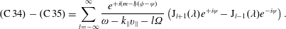 $$\begin{eqnarray}\displaystyle (\text{C}\,34)-(\text{C}\,35)=\mathop{\sum }_{l=-\infty }^{\infty }\frac{e^{+i(m-l)(\unicode[STIX]{x1D719}-\unicode[STIX]{x1D713})}}{\unicode[STIX]{x1D714}-k_{\Vert }v_{\Vert }-l\unicode[STIX]{x1D6FA}}\left(\text{J}_{l+1}(\unicode[STIX]{x1D706})e^{+i\unicode[STIX]{x1D713}}-\text{J}_{l-1}(\unicode[STIX]{x1D706})e^{-i\unicode[STIX]{x1D713}}\right). & & \displaystyle\end{eqnarray}$$
The terms proportional to
 $E_{z}$
are now very easy to transform and
$E_{z}$
are now very easy to transform and
 $$\begin{eqnarray}\displaystyle & & \displaystyle \mathop{\sum }_{n=-\infty }^{\infty }e^{+i(m-n)(\unicode[STIX]{x1D719}-\unicode[STIX]{x1D713})}\text{J}_{n}(\unicode[STIX]{x1D706})\frac{e^{i(\unicode[STIX]{x1D719}-\unicode[STIX]{x1D713})}}{\unicode[STIX]{x1D714}-k_{\Vert }v_{\Vert }-(n-1)\unicode[STIX]{x1D6FA}}\nonumber\\ \displaystyle & & \displaystyle \qquad =\mathop{\sum }_{l=-\infty }^{\infty }e^{+i(m-l)(\unicode[STIX]{x1D719}-\unicode[STIX]{x1D713})}\text{J}_{l+1}(\unicode[STIX]{x1D706})\frac{1}{\unicode[STIX]{x1D714}-k_{\Vert }v_{\Vert }-l\unicode[STIX]{x1D6FA}};\end{eqnarray}$$
 $$\begin{eqnarray}\displaystyle & & \displaystyle \mathop{\sum }_{n=-\infty }^{\infty }e^{+i(m-n)(\unicode[STIX]{x1D719}-\unicode[STIX]{x1D713})}\text{J}_{n}(\unicode[STIX]{x1D706})\frac{e^{-i(\unicode[STIX]{x1D719}-\unicode[STIX]{x1D713})}}{\unicode[STIX]{x1D714}-k_{\Vert }v_{\Vert }-(n+1)\unicode[STIX]{x1D6FA}}\nonumber\\ \displaystyle & & \displaystyle \qquad =\mathop{\sum }_{l=-\infty }^{\infty }e^{+i(m-l)(\unicode[STIX]{x1D719}-\unicode[STIX]{x1D713})}\text{J}_{l-1}(\unicode[STIX]{x1D706})\frac{1}{\unicode[STIX]{x1D714}-k_{\Vert }v_{\Vert }-l\unicode[STIX]{x1D6FA}},\end{eqnarray}$$
and together
 $$\begin{eqnarray}\displaystyle (\text{C}\,38)+(\text{C}\,39)=\mathop{\sum }_{l=-\infty }^{\infty }\frac{e^{+i(m-l)(\unicode[STIX]{x1D719}-\unicode[STIX]{x1D713})}}{\unicode[STIX]{x1D714}-k_{\Vert }v_{\Vert }-l\unicode[STIX]{x1D6FA}}\left(\text{J}_{l+1}(\unicode[STIX]{x1D706})+\text{J}_{l-1}(\unicode[STIX]{x1D706})\right). & & \displaystyle\end{eqnarray}$$
We therefore managed to rearrange the summation and equation (C 33) for
 $f^{(1)}$
transforms to
$f^{(1)}$
transforms to
 $$\begin{eqnarray}\displaystyle f^{(1)} & = & \displaystyle -\frac{q_{r}}{m_{r}}\mathop{\sum }_{l=-\infty }^{\infty }\mathop{\sum }_{m=-\infty }^{\infty }\frac{e^{+i(m-l)(\unicode[STIX]{x1D719}-\unicode[STIX]{x1D713})}}{\unicode[STIX]{x1D714}-k_{\Vert }v_{\Vert }-l\unicode[STIX]{x1D6FA}}\text{J}_{m}(\unicode[STIX]{x1D706})\left\{\left[\frac{iE_{x}}{2}\left(\text{J}_{l+1}(\unicode[STIX]{x1D706})e^{+i\unicode[STIX]{x1D713}}+\text{J}_{l-1}(\unicode[STIX]{x1D706})e^{-i\unicode[STIX]{x1D713}}\right)\right.\right.\nonumber\\ \displaystyle & & \displaystyle \left.+\,\frac{E_{y}}{2}\left(\text{J}_{l+1}(\unicode[STIX]{x1D706})e^{+i\unicode[STIX]{x1D713}}-\text{J}_{l-1}(\unicode[STIX]{x1D706})e^{-i\unicode[STIX]{x1D713}}\right)\right]\left[\left(1-\frac{v_{\Vert }k_{\Vert }}{\unicode[STIX]{x1D714}}\right)\frac{\unicode[STIX]{x2202}f_{0}}{\unicode[STIX]{x2202}v_{\bot }}+\frac{k_{\Vert }v_{\bot }}{\unicode[STIX]{x1D714}}\frac{\unicode[STIX]{x2202}f_{0}}{\unicode[STIX]{x2202}v_{\Vert }}\right]\nonumber\\ \displaystyle & & \displaystyle \left.+\,E_{z}\left[i\text{J}_{l}(\unicode[STIX]{x1D706})\frac{\unicode[STIX]{x2202}f_{0}}{\unicode[STIX]{x2202}v_{\Vert }}+\frac{k_{\bot }}{\unicode[STIX]{x1D714}}\left(v_{\Vert }\frac{\unicode[STIX]{x2202}f_{0}}{\unicode[STIX]{x2202}v_{\bot }}-v_{\bot }\frac{\unicode[STIX]{x2202}f_{0}}{\unicode[STIX]{x2202}v_{\Vert }}\right)\frac{i}{2}\left(\text{J}_{l+1}(\unicode[STIX]{x1D706})+\text{J}_{l-1}(\unicode[STIX]{x1D706})\right)\right]\right\}.\qquad\end{eqnarray}$$
This is much prettier result than (C 33) since all the cyclotron resonances of the same order are nicely grouped together. We are essentially done, however, there is one more step that allows further simplification and that is the use of Bessel identities
 $$\begin{eqnarray}\displaystyle & \displaystyle \text{J}_{l-1}(z)+\text{J}_{l+1}(z)=\frac{2l}{z}\text{J}_{l}(z); & \displaystyle\end{eqnarray}$$
 $$\begin{eqnarray}\displaystyle & \displaystyle \text{J}_{l-1}(z)-\text{J}_{l+1}(z)=2\text{J}_{l}^{\prime }(z), & \displaystyle\end{eqnarray}$$
where the prime represents a derivative, so
 $\text{J}_{l}^{\prime }(z)=\unicode[STIX]{x2202}\text{J}_{l}(z)/\unicode[STIX]{x2202}z$
. The contributions proportional to
$\text{J}_{l}^{\prime }(z)=\unicode[STIX]{x2202}\text{J}_{l}(z)/\unicode[STIX]{x2202}z$
. The contributions proportional to
 $E_{x}$
,
$E_{x}$
,
 $E_{y}$
are rewritten as
$E_{y}$
are rewritten as
 $$\begin{eqnarray}\displaystyle \text{J}_{l+1}(\unicode[STIX]{x1D706})e^{+i\unicode[STIX]{x1D713}}+\text{J}_{l-1}(\unicode[STIX]{x1D706})e^{-i\unicode[STIX]{x1D713}} & = & \displaystyle \text{J}_{l+1}(\unicode[STIX]{x1D706})(\cos \unicode[STIX]{x1D713}+i\sin \unicode[STIX]{x1D713})+\text{J}_{l-1}(\unicode[STIX]{x1D706})(\cos \unicode[STIX]{x1D713}-i\sin \unicode[STIX]{x1D713})\nonumber\\ \displaystyle & = & \displaystyle \left(\text{J}_{l+1}(\unicode[STIX]{x1D706})+\text{J}_{l-1}(\unicode[STIX]{x1D706})\right)\cos \unicode[STIX]{x1D713}+i\left(\text{J}_{l+1}(\unicode[STIX]{x1D706})-\text{J}_{l-1}(\unicode[STIX]{x1D706})\right)\sin \unicode[STIX]{x1D713}\nonumber\\ \displaystyle & = & \displaystyle \frac{2l}{\unicode[STIX]{x1D706}}\text{J}_{l}(\unicode[STIX]{x1D706})\cos \unicode[STIX]{x1D713}-2i\text{J}_{l}^{\prime }(\unicode[STIX]{x1D706})\sin \unicode[STIX]{x1D713};\end{eqnarray}$$
 $$\begin{eqnarray}\displaystyle \text{J}_{l+1}(\unicode[STIX]{x1D706})e^{+i\unicode[STIX]{x1D713}}-\text{J}_{l-1}(\unicode[STIX]{x1D706})e^{-i\unicode[STIX]{x1D713}} & = & \displaystyle \text{J}_{l+1}(\unicode[STIX]{x1D706})(\cos \unicode[STIX]{x1D713}+i\sin \unicode[STIX]{x1D713})-\text{J}_{l-1}(\unicode[STIX]{x1D706})(\cos \unicode[STIX]{x1D713}-i\sin \unicode[STIX]{x1D713})\nonumber\\ \displaystyle & = & \displaystyle \left(\text{J}_{l+1}(\unicode[STIX]{x1D706})-\text{J}_{l-1}(\unicode[STIX]{x1D706})\right)\cos \unicode[STIX]{x1D713}+i\left(\text{J}_{l+1}(\unicode[STIX]{x1D706})+\text{J}_{l-1}(\unicode[STIX]{x1D706})\right)\sin \unicode[STIX]{x1D713}\nonumber\\ \displaystyle & = & \displaystyle -2\text{J}_{l}^{\prime }(\unicode[STIX]{x1D706})\cos \unicode[STIX]{x1D713}+i\frac{2l}{\unicode[STIX]{x1D706}}\text{J}_{l}(\unicode[STIX]{x1D706})\sin \unicode[STIX]{x1D713},\end{eqnarray}$$
and the contributions proportional to
 $E_{z}$
are trivial. The expression for
$E_{z}$
are trivial. The expression for
 $f^{(1)}$
reads
$f^{(1)}$
reads
 $$\begin{eqnarray}\displaystyle f^{(1)} & = & \displaystyle -\frac{q_{r}}{m_{r}}\mathop{\sum }_{l=-\infty }^{\infty }\mathop{\sum }_{m=-\infty }^{\infty }\frac{e^{+i(m-l)(\unicode[STIX]{x1D719}-\unicode[STIX]{x1D713})}}{\unicode[STIX]{x1D714}-k_{\Vert }v_{\Vert }-l\unicode[STIX]{x1D6FA}}\text{J}_{m}(\unicode[STIX]{x1D706})\left\{\left[iE_{x}\left(\frac{l}{\unicode[STIX]{x1D706}}\text{J}_{l}(\unicode[STIX]{x1D706})\cos \unicode[STIX]{x1D713}-i\text{J}_{l}^{\prime }(\unicode[STIX]{x1D706})\sin \unicode[STIX]{x1D713}\right)\right.\right.\nonumber\\ \displaystyle & & \displaystyle \left.+\,iE_{y}\left(i\text{J}_{l}^{\prime }(\unicode[STIX]{x1D706})\cos \unicode[STIX]{x1D713}+\frac{l}{\unicode[STIX]{x1D706}}\text{J}_{l}(\unicode[STIX]{x1D706})\sin \unicode[STIX]{x1D713}\right)\right]\left[\left(1-\frac{v_{\Vert }k_{\Vert }}{\unicode[STIX]{x1D714}}\right)\frac{\unicode[STIX]{x2202}f_{0}}{\unicode[STIX]{x2202}v_{\bot }}+\frac{k_{\Vert }v_{\bot }}{\unicode[STIX]{x1D714}}\frac{\unicode[STIX]{x2202}f_{0}}{\unicode[STIX]{x2202}v_{\Vert }}\right]\nonumber\\ \displaystyle & & \displaystyle \left.+\,iE_{z}\text{J}_{l}(\unicode[STIX]{x1D706})\left[\frac{\unicode[STIX]{x2202}f_{0}}{\unicode[STIX]{x2202}v_{\Vert }}+\frac{k_{\bot }}{\unicode[STIX]{x1D714}}\frac{l}{\unicode[STIX]{x1D706}}\left(v_{\Vert }\frac{\unicode[STIX]{x2202}f_{0}}{\unicode[STIX]{x2202}v_{\bot }}-v_{\bot }\frac{\unicode[STIX]{x2202}f_{0}}{\unicode[STIX]{x2202}v_{\Vert }}\right)\right]\right\}.\end{eqnarray}$$
Pulling the
 $i$
out to the front, re-grouping the
$i$
out to the front, re-grouping the
 $E_{x},E_{y}$
terms together and renaming
$E_{x},E_{y}$
terms together and renaming
 $l\rightarrow n$
(since it is somewhat nicer and cannot be confused with imaginary
$l\rightarrow n$
(since it is somewhat nicer and cannot be confused with imaginary
 $i$
, even though it can be confused with density
$i$
, even though it can be confused with density
 $n_{r}$
), together with reintroducing the species index
$n_{r}$
), together with reintroducing the species index
 $r$
for
$r$
for
 $f_{r}^{(1)}$
,
$f_{r}^{(1)}$
,
 $f_{0r}$
,
$f_{0r}$
,
 $\unicode[STIX]{x1D706}_{r}$
and
$\unicode[STIX]{x1D706}_{r}$
and
 $\unicode[STIX]{x1D6FA}_{r}$
, yields the ‘grand-finale’ result of this section, in the form
$\unicode[STIX]{x1D6FA}_{r}$
, yields the ‘grand-finale’ result of this section, in the form
 $$\begin{eqnarray}\displaystyle f_{r}^{(1)} & = & \displaystyle -\frac{iq_{r}}{m_{r}}\mathop{\sum }_{n=-\infty }^{\infty }\mathop{\sum }_{m=-\infty }^{\infty }\frac{e^{+i(m-n)(\unicode[STIX]{x1D719}-\unicode[STIX]{x1D713})}}{\unicode[STIX]{x1D714}-k_{\Vert }v_{\Vert }-n\unicode[STIX]{x1D6FA}_{r}}\text{J}_{m}(\unicode[STIX]{x1D706}_{r})\left\{\left[\frac{n\text{J}_{n}(\unicode[STIX]{x1D706}_{r})}{\unicode[STIX]{x1D706}_{r}}\left(E_{x}\cos \unicode[STIX]{x1D713}+E_{y}\sin \unicode[STIX]{x1D713}\right)\right.\right.\nonumber\\ \displaystyle & & \displaystyle \left.\vphantom{\frac{n\text{J}_{n}(\unicode[STIX]{x1D706}_{r})}{\unicode[STIX]{x1D706}_{r}}}+\,i\text{J}_{n}^{\prime }(\unicode[STIX]{x1D706}_{r})\left(-E_{x}\sin \unicode[STIX]{x1D713}+E_{y}\cos \unicode[STIX]{x1D713}\right)\right]\left[\left(1-\frac{k_{\Vert }v_{\Vert }}{\unicode[STIX]{x1D714}}\right)\frac{\unicode[STIX]{x2202}f_{0r}}{\unicode[STIX]{x2202}v_{\bot }}+\frac{k_{\Vert }v_{\bot }}{\unicode[STIX]{x1D714}}\frac{\unicode[STIX]{x2202}f_{0r}}{\unicode[STIX]{x2202}v_{\Vert }}\right]\nonumber\\ \displaystyle & & \displaystyle \left.+\,E_{z}\text{J}_{n}(\unicode[STIX]{x1D706}_{r})\left[\frac{\unicode[STIX]{x2202}f_{0r}}{\unicode[STIX]{x2202}v_{\Vert }}-\frac{n\unicode[STIX]{x1D6FA}_{r}}{\unicode[STIX]{x1D714}}\left(\frac{\unicode[STIX]{x2202}f_{0r}}{\unicode[STIX]{x2202}v_{\Vert }}-\frac{v_{\Vert }}{v_{\bot }}\frac{\unicode[STIX]{x2202}f_{0r}}{\unicode[STIX]{x2202}v_{\bot }}\right)\right]\right\}.\end{eqnarray}$$
The quantity
 $\unicode[STIX]{x1D706}_{r}\equiv k_{\bot }v_{\bot }/\unicode[STIX]{x1D6FA}_{r}$
, and
$\unicode[STIX]{x1D706}_{r}\equiv k_{\bot }v_{\bot }/\unicode[STIX]{x1D6FA}_{r}$
, and
 $\unicode[STIX]{x1D6FA}_{r}=q_{r}B_{0}/(m_{r}c)$
. The expression is equivalent to equation (4.88) in Swanson.Footnote
13
$\unicode[STIX]{x1D6FA}_{r}=q_{r}B_{0}/(m_{r}c)$
. The expression is equivalent to equation (4.88) in Swanson.Footnote
13
C.1 Case
$\unicode[STIX]{x1D713}=0$
, propagation in the
$x{-}z$
plane


If we are interested only in linear dispersion relations (and not in the development of higher-order fluid hierarchy suitable for numerical simulations), we can restrict ourselves to the propagation in the
 $x{-}z$
plane, as we have done many times before when solving dispersion relations. In the
$x{-}z$
plane, as we have done many times before when solving dispersion relations. In the
 $x{-}z$
plane, the wavenumber
$x{-}z$
plane, the wavenumber
 $\boldsymbol{k}=(k_{x},0,k_{z})=(k_{\bot },0,k_{\Vert })$
, or equivalently the angle
$\boldsymbol{k}=(k_{x},0,k_{z})=(k_{\bot },0,k_{\Vert })$
, or equivalently the angle
 $\unicode[STIX]{x1D713}=0$
. In this case, the expression (C 47) simplifies to
$\unicode[STIX]{x1D713}=0$
. In this case, the expression (C 47) simplifies to
 $$\begin{eqnarray}\displaystyle f_{r}^{(1)} & = & \displaystyle -\frac{iq_{r}}{m_{r}}\mathop{\sum }_{n=-\infty }^{\infty }\mathop{\sum }_{m=-\infty }^{\infty }\frac{e^{i(m-n)\unicode[STIX]{x1D719}}}{\unicode[STIX]{x1D714}-k_{\Vert }v_{\Vert }-n\unicode[STIX]{x1D6FA}_{r}}\text{J}_{m}(\unicode[STIX]{x1D706}_{r})\nonumber\\ \displaystyle & & \displaystyle \times \,\left\{\left[\frac{n\text{J}_{n}(\unicode[STIX]{x1D706}_{r})}{\unicode[STIX]{x1D706}_{r}}E_{x}+i\text{J}_{n}^{\prime }(\unicode[STIX]{x1D706}_{r})E_{y}\right]\left[\left(1-\frac{k_{\Vert }v_{\Vert }}{\unicode[STIX]{x1D714}}\right)\frac{\unicode[STIX]{x2202}f_{0r}}{\unicode[STIX]{x2202}v_{\bot }}+\frac{k_{\Vert }v_{\bot }}{\unicode[STIX]{x1D714}}\frac{\unicode[STIX]{x2202}f_{0r}}{\unicode[STIX]{x2202}v_{\Vert }}\right]\right.\nonumber\\ \displaystyle & & \displaystyle \left.+\,E_{z}\text{J}_{n}(\unicode[STIX]{x1D706}_{r})\left[\frac{\unicode[STIX]{x2202}f_{0r}}{\unicode[STIX]{x2202}v_{\Vert }}-\frac{n\unicode[STIX]{x1D6FA}_{r}}{\unicode[STIX]{x1D714}v_{\bot }}\left(v_{\bot }\frac{\unicode[STIX]{x2202}f_{0r}}{\unicode[STIX]{x2202}v_{\Vert }}-v_{\Vert }\frac{\unicode[STIX]{x2202}f_{0r}}{\unicode[STIX]{x2202}v_{\bot }}\right)\right]\right\},\end{eqnarray}$$
which is equivalent to the equation (10.3.12) in Gurnett and Bhattacharjee. In this case, the coupling of the electric field components with the sum over index
 $m$
disappears, and the sum can be left in its original form
$m$
disappears, and the sum can be left in its original form
 $\sum _{m=-\infty }^{\infty }e^{+im\unicode[STIX]{x1D719}}\text{J}_{m}(\unicode[STIX]{x1D706})=e^{+i\unicode[STIX]{x1D706}\sin \unicode[STIX]{x1D719}}$
, yielding
$\sum _{m=-\infty }^{\infty }e^{+im\unicode[STIX]{x1D719}}\text{J}_{m}(\unicode[STIX]{x1D706})=e^{+i\unicode[STIX]{x1D706}\sin \unicode[STIX]{x1D719}}$
, yielding
 $$\begin{eqnarray}\displaystyle f_{r}^{(1)} & = & \displaystyle -\frac{iq_{r}}{m_{r}}e^{i\unicode[STIX]{x1D706}_{r}\sin \unicode[STIX]{x1D719}}\mathop{\sum }_{n=-\infty }^{\infty }\frac{e^{-in\unicode[STIX]{x1D719}}}{\unicode[STIX]{x1D714}-k_{\Vert }v_{\Vert }-n\unicode[STIX]{x1D6FA}_{r}}\nonumber\\ \displaystyle & & \displaystyle \times \,\left\{\left[\frac{n\text{J}_{n}(\unicode[STIX]{x1D706}_{r})}{\unicode[STIX]{x1D706}_{r}}E_{x}+i\text{J}_{n}^{\prime }(\unicode[STIX]{x1D706}_{r})E_{y}\right]\left[\left(1-\frac{k_{\Vert }v_{\Vert }}{\unicode[STIX]{x1D714}}\right)\frac{\unicode[STIX]{x2202}f_{0r}}{\unicode[STIX]{x2202}v_{\bot }}+\frac{k_{\Vert }v_{\bot }}{\unicode[STIX]{x1D714}}\frac{\unicode[STIX]{x2202}f_{0r}}{\unicode[STIX]{x2202}v_{\Vert }}\right]\right.\nonumber\\ \displaystyle & & \displaystyle \left.+\,E_{z}\text{J}_{n}(\unicode[STIX]{x1D706}_{r})\left[\frac{\unicode[STIX]{x2202}f_{0r}}{\unicode[STIX]{x2202}v_{\Vert }}-\frac{n\unicode[STIX]{x1D6FA}_{r}}{\unicode[STIX]{x1D714}v_{\bot }}\left(v_{\bot }\frac{\unicode[STIX]{x2202}f_{0r}}{\unicode[STIX]{x2202}v_{\Vert }}-v_{\Vert }\frac{\unicode[STIX]{x2202}f_{0r}}{\unicode[STIX]{x2202}v_{\bot }}\right)\right]\right\}.\end{eqnarray}$$
If the last term proportional to
 $E_{z}$
is compared with the expression (5.2.1.9) of Akhiezer, it appears that Akhiezer has a typo, where instead of the correct
$E_{z}$
is compared with the expression (5.2.1.9) of Akhiezer, it appears that Akhiezer has a typo, where instead of the correct
 $v_{\bot }$
there is a typo
$v_{\bot }$
there is a typo
 $v_{\Vert }$
.
$v_{\Vert }$
.
C.2 General
$f^{(1)}$
for a bi-Maxwellian distribution

Prescribing
 $f_{0}$
to be a bi-Maxwellian distribution function, the general expression (C 47) for
$f_{0}$
to be a bi-Maxwellian distribution function, the general expression (C 47) for
 $f^{(1)}$
further simplifies. Since in the Vlasov expansion the gyrotropic
$f^{(1)}$
further simplifies. Since in the Vlasov expansion the gyrotropic
 $f_{0}$
was assumed to dependent only on
$f_{0}$
was assumed to dependent only on
 $\boldsymbol{v}$
, i.e.
$\boldsymbol{v}$
, i.e.
 $f_{0}(v_{\bot }^{2},v_{\Vert }^{2})$
and be
$f_{0}(v_{\bot }^{2},v_{\Vert }^{2})$
and be
 $\boldsymbol{x},t$
independent, the fluid velocity
$\boldsymbol{x},t$
independent, the fluid velocity
 $\boldsymbol{u}$
is removed from the distribution function and the ‘pure’ bi-Maxwellian is
$\boldsymbol{u}$
is removed from the distribution function and the ‘pure’ bi-Maxwellian is
 $$\begin{eqnarray}\displaystyle f_{0}=n_{0r}\sqrt{\frac{\unicode[STIX]{x1D6FC}_{\Vert }}{\unicode[STIX]{x03C0}}}\frac{\unicode[STIX]{x1D6FC}_{\bot }}{\unicode[STIX]{x03C0}}e^{-\unicode[STIX]{x1D6FC}_{\Vert }v_{\Vert }^{2}-\unicode[STIX]{x1D6FC}_{\bot }v_{\bot }^{2}}, & & \displaystyle\end{eqnarray}$$
where
 $\unicode[STIX]{x1D6FC}_{\Vert }\equiv m/(2T_{\Vert }^{(0)})$
,
$\unicode[STIX]{x1D6FC}_{\Vert }\equiv m/(2T_{\Vert }^{(0)})$
,
 $\unicode[STIX]{x1D6FC}_{\bot }=m/(2T_{\bot }^{(0)})$
, or in the language of thermal speeds,
$\unicode[STIX]{x1D6FC}_{\bot }=m/(2T_{\bot }^{(0)})$
, or in the language of thermal speeds,
 $v_{\text{th}\Vert }^{2}=2T_{\Vert }^{(0)}/m=\unicode[STIX]{x1D6FC}_{\Vert }^{-1}$
and
$v_{\text{th}\Vert }^{2}=2T_{\Vert }^{(0)}/m=\unicode[STIX]{x1D6FC}_{\Vert }^{-1}$
and
 $v_{\text{th}\bot }^{2}=2T_{\bot }^{(0)}/m=\unicode[STIX]{x1D6FC}_{\bot }^{-1}$
. We prefer the
$v_{\text{th}\bot }^{2}=2T_{\bot }^{(0)}/m=\unicode[STIX]{x1D6FC}_{\bot }^{-1}$
. We prefer the
 $\unicode[STIX]{x1D6FC}$
notation instead of the thermal speed
$\unicode[STIX]{x1D6FC}$
notation instead of the thermal speed
 $v_{\text{th}}$
, since in long analytic calculations, there is a lesser chance of an error.
$v_{\text{th}}$
, since in long analytic calculations, there is a lesser chance of an error.
It is straightforward to calculate that for a bi-Maxwellian
 $$\begin{eqnarray}\displaystyle & \displaystyle \frac{\unicode[STIX]{x2202}f_{0}}{\unicode[STIX]{x2202}v_{\Vert }}=-2\unicode[STIX]{x1D6FC}_{\Vert }v_{\Vert }\,f_{0}=-\frac{m_{r}}{T_{\Vert }^{(0)}}v_{\Vert }\,f_{0}; & \displaystyle\end{eqnarray}$$
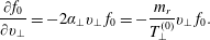 $$\begin{eqnarray}\displaystyle & \displaystyle \frac{\unicode[STIX]{x2202}f_{0}}{\unicode[STIX]{x2202}v_{\bot }}=-2\unicode[STIX]{x1D6FC}_{\bot }v_{\bot }\,f_{0}=-\frac{m_{r}}{T_{\bot }^{(0)}}v_{\bot }\,f_{0}. & \displaystyle\end{eqnarray}$$
The bi-Maxwellian distribution
 $f_{0}$
therefore can be pulled out (together with
$f_{0}$
therefore can be pulled out (together with
 $-m_{r}$
) and the general expression (C 47) rewrites
$-m_{r}$
) and the general expression (C 47) rewrites
 $$\begin{eqnarray}\displaystyle f_{r}^{(1)} & = & \displaystyle iq_{r}f_{0r}\mathop{\sum }_{n=-\infty }^{\infty }\mathop{\sum }_{m=-\infty }^{\infty }\frac{e^{+i(m-n)(\unicode[STIX]{x1D719}-\unicode[STIX]{x1D713})}}{\unicode[STIX]{x1D714}-k_{\Vert }v_{\Vert }-n\unicode[STIX]{x1D6FA}_{r}}\text{J}_{m}(\unicode[STIX]{x1D706}_{r})\left\{\left[n\text{J}_{n}(\unicode[STIX]{x1D706}_{r})\frac{\unicode[STIX]{x1D6FA}_{r}}{k_{\bot }}\left(E_{x}\cos \unicode[STIX]{x1D713}+E_{y}\sin \unicode[STIX]{x1D713}\right)\right.\right.\nonumber\\ \displaystyle & & \displaystyle \left.\vphantom{\frac{\unicode[STIX]{x1D6FA}_{r}}{k_{\bot }}}+\,i\text{J}_{n}^{\prime }(\unicode[STIX]{x1D706}_{r})v_{\bot }\left(-E_{x}\sin \unicode[STIX]{x1D713}+E_{y}\cos \unicode[STIX]{x1D713}\right)\right]\left[\frac{1}{T_{\bot r}^{(0)}}+\frac{k_{\Vert }v_{\Vert }}{\unicode[STIX]{x1D714}}\left(\frac{1}{T_{\Vert r}^{(0)}}-\frac{1}{T_{\bot r}^{(0)}}\right)\right]\nonumber\\ \displaystyle & & \displaystyle \left.+\,E_{z}\text{J}_{n}(\unicode[STIX]{x1D706}_{r})v_{\Vert }\left[\frac{1}{T_{\Vert r}^{(0)}}-\frac{n\unicode[STIX]{x1D6FA}_{r}}{\unicode[STIX]{x1D714}}\left(\frac{1}{T_{\Vert r}^{(0)}}-\frac{1}{T_{\bot r}^{(0)}}\right)\right]\right\}.\end{eqnarray}$$
C.3 General
$f^{(1)}$
for a bi-kappa distribution

A bi-kappa distribution function (as used previously in Part 1 of the manuscript) reads
 $$\begin{eqnarray}f_{0}=n_{0r}\frac{\unicode[STIX]{x1D6E4}(\unicode[STIX]{x1D705}+1)}{\unicode[STIX]{x1D6E4}(\unicode[STIX]{x1D705}-\frac{1}{2})}\sqrt{\frac{\unicode[STIX]{x1D6FC}_{\Vert }}{\unicode[STIX]{x03C0}}}\frac{\unicode[STIX]{x1D6FC}_{\bot }}{\unicode[STIX]{x03C0}}\left[1+\unicode[STIX]{x1D6FC}_{\Vert }v_{\Vert }^{2}+\unicode[STIX]{x1D6FC}_{\bot }v_{\bot }^{2}\right]^{-(\unicode[STIX]{x1D705}+1)},\end{eqnarray}$$
where the abbreviated
 $\unicode[STIX]{x1D6FC}_{\Vert }=1/(\unicode[STIX]{x1D705}\unicode[STIX]{x1D703}_{\Vert }^{2})$
,
$\unicode[STIX]{x1D6FC}_{\Vert }=1/(\unicode[STIX]{x1D705}\unicode[STIX]{x1D703}_{\Vert }^{2})$
,
 $\unicode[STIX]{x1D6FC}_{\bot }=1/(\unicode[STIX]{x1D705}\unicode[STIX]{x1D703}_{\bot }^{2})$
and the thermal speeds are
$\unicode[STIX]{x1D6FC}_{\bot }=1/(\unicode[STIX]{x1D705}\unicode[STIX]{x1D703}_{\bot }^{2})$
and the thermal speeds are
 $\unicode[STIX]{x1D703}_{\Vert }^{2}=(1-3/(2\unicode[STIX]{x1D705}))(2T_{\Vert r}^{(0)}/m_{r})$
,
$\unicode[STIX]{x1D703}_{\Vert }^{2}=(1-3/(2\unicode[STIX]{x1D705}))(2T_{\Vert r}^{(0)}/m_{r})$
,
 $\unicode[STIX]{x1D703}_{\bot }^{2}=(1-3/(2\unicode[STIX]{x1D705}))(2T_{\bot r}^{(0)}/m_{r})$
. We have again emphasized the species index
$\unicode[STIX]{x1D703}_{\bot }^{2}=(1-3/(2\unicode[STIX]{x1D705}))(2T_{\bot r}^{(0)}/m_{r})$
. We have again emphasized the species index
 $r$
only where necessary, even though in the final expression for
$r$
only where necessary, even though in the final expression for
 $f^{(1)}$
we will use the proper
$f^{(1)}$
we will use the proper
 $\unicode[STIX]{x1D6FC}_{\Vert r}$
,
$\unicode[STIX]{x1D6FC}_{\Vert r}$
,
 $\unicode[STIX]{x1D6FC}_{\bot r}$
. Also, the
$\unicode[STIX]{x1D6FC}_{\bot r}$
. Also, the
 $\unicode[STIX]{x1D705}$
-index should be written as
$\unicode[STIX]{x1D705}$
-index should be written as
 $\unicode[STIX]{x1D705}_{r}$
, since the index will be different for each particle species. The derivatives of
$\unicode[STIX]{x1D705}_{r}$
, since the index will be different for each particle species. The derivatives of
 $f_{0}$
are
$f_{0}$
are
 $$\begin{eqnarray}\displaystyle & \displaystyle \frac{\unicode[STIX]{x2202}f_{0}}{\unicode[STIX]{x2202}v_{\Vert }}=-\frac{2(\unicode[STIX]{x1D705}+1)\unicode[STIX]{x1D6FC}_{\Vert }v_{\Vert }}{1+\unicode[STIX]{x1D6FC}_{\Vert }v_{\Vert }^{2}+\unicode[STIX]{x1D6FC}_{\bot }v_{\bot }^{2}}f_{0}; & \displaystyle\end{eqnarray}$$
 $$\begin{eqnarray}\displaystyle & \displaystyle \frac{\unicode[STIX]{x2202}f_{0}}{\unicode[STIX]{x2202}v_{\bot }}=-\frac{2(\unicode[STIX]{x1D705}+1)\unicode[STIX]{x1D6FC}_{\bot }v_{\bot }}{1+\unicode[STIX]{x1D6FC}_{\Vert }v_{\Vert }^{2}+\unicode[STIX]{x1D6FC}_{\bot }v_{\bot }^{2}}f_{0}, & \displaystyle\end{eqnarray}$$
which yields the
 $f^{(1)}$
for a bi-kappa distribution
$f^{(1)}$
for a bi-kappa distribution
 $$\begin{eqnarray}\displaystyle f_{r}^{(1)} & = & \displaystyle \frac{iq_{r}}{m_{r}}\frac{2(\unicode[STIX]{x1D705}_{r}+1)f_{0r}}{(1+\unicode[STIX]{x1D6FC}_{\Vert r}v_{\Vert }^{2}+\unicode[STIX]{x1D6FC}_{\bot r}v_{\bot }^{2})}\mathop{\sum }_{n=-\infty }^{\infty }\mathop{\sum }_{m=-\infty }^{\infty }\frac{e^{+i(m-n)(\unicode[STIX]{x1D719}-\unicode[STIX]{x1D713})}}{\unicode[STIX]{x1D714}-k_{\Vert }v_{\Vert }-n\unicode[STIX]{x1D6FA}_{r}}\text{J}_{m}(\unicode[STIX]{x1D706}_{r})\nonumber\\ \displaystyle & & \displaystyle \times \,\left\{\left[n\text{J}_{n}(\unicode[STIX]{x1D706}_{r})\frac{\unicode[STIX]{x1D6FA}_{r}}{k_{\bot }}\left(E_{x}\cos \unicode[STIX]{x1D713}+E_{y}\sin \unicode[STIX]{x1D713}\right)\right.\right.\nonumber\\ \displaystyle & & \displaystyle \left.\vphantom{\frac{\unicode[STIX]{x1D6FA}_{r}}{k_{\bot }}}+\,i\text{J}_{n}^{\prime }(\unicode[STIX]{x1D706}_{r})v_{\bot }\left(-E_{x}\sin \unicode[STIX]{x1D713}+E_{y}\cos \unicode[STIX]{x1D713}\right)\right]\left[\unicode[STIX]{x1D6FC}_{\bot r}+\frac{k_{\Vert }v_{\Vert }}{\unicode[STIX]{x1D714}}(\unicode[STIX]{x1D6FC}_{\Vert r}-\unicode[STIX]{x1D6FC}_{\bot r})\right]\nonumber\\ \displaystyle & & \displaystyle \left.+\,E_{z}\text{J}_{n}(\unicode[STIX]{x1D706}_{r})v_{\Vert }\left[\unicode[STIX]{x1D6FC}_{\Vert r}-\frac{n\unicode[STIX]{x1D6FA}_{r}}{\unicode[STIX]{x1D714}}\left(\unicode[STIX]{x1D6FC}_{\Vert r}-\unicode[STIX]{x1D6FC}_{\bot r}\right)\right]\right\}.\end{eqnarray}$$
In the limit
 $\unicode[STIX]{x1D705}\rightarrow \infty$
, (C 57) should ‘obviously’ converge to the bi-Maxwellian (C 53).
$\unicode[STIX]{x1D705}\rightarrow \infty$
, (C 57) should ‘obviously’ converge to the bi-Maxwellian (C 53).
C.4 Formulation with scalar potentials
$\unicode[STIX]{x1D6F7},\unicode[STIX]{x1D6F9}$

In kinetic theory and especially in the formulation of Landau fluid models, instead of electric fields, it is often useful to work with scalar potentials
 $\unicode[STIX]{x1D6F7},\unicode[STIX]{x1D6F9}$
, that should not be confused with azimuthal angles
$\unicode[STIX]{x1D6F7},\unicode[STIX]{x1D6F9}$
, that should not be confused with azimuthal angles
 $\unicode[STIX]{x1D719},\unicode[STIX]{x1D713}$
for the velocity and wavenumber in the cylindrical coordinate system. The usual decomposition employs the scalar potential
$\unicode[STIX]{x1D719},\unicode[STIX]{x1D713}$
for the velocity and wavenumber in the cylindrical coordinate system. The usual decomposition employs the scalar potential
 $\unicode[STIX]{x1D6F7}$
and the vector potential
$\unicode[STIX]{x1D6F7}$
and the vector potential
 $\boldsymbol{A}$
, according to
$\boldsymbol{A}$
, according to
 $$\begin{eqnarray}\displaystyle & \displaystyle \boldsymbol{B}=\boldsymbol{B}_{0}+\unicode[STIX]{x1D735}\times \boldsymbol{A}; & \displaystyle\end{eqnarray}$$
 $$\begin{eqnarray}\displaystyle & \displaystyle \boldsymbol{E}=-\unicode[STIX]{x1D735}\unicode[STIX]{x1D6F7}-\frac{1}{c}\frac{\unicode[STIX]{x2202}\boldsymbol{A}}{\unicode[STIX]{x2202}t}, & \displaystyle\end{eqnarray}$$
and it is useful to choose the Coulomb gauge
 $\unicode[STIX]{x1D735}\boldsymbol{\cdot }\boldsymbol{A}=0$
. By exploring the equation for
$\unicode[STIX]{x1D735}\boldsymbol{\cdot }\boldsymbol{A}=0$
. By exploring the equation for
 $f^{(1)}$
, it is noteworthy that the perpendicular electric fields
$f^{(1)}$
, it is noteworthy that the perpendicular electric fields
 $E_{x},E_{y}$
are ‘coupled’ through the azimuthal angle
$E_{x},E_{y}$
are ‘coupled’ through the azimuthal angle
 $\unicode[STIX]{x1D713}$
. In contrast, the parallel electric field component
$\unicode[STIX]{x1D713}$
. In contrast, the parallel electric field component
 $E_{z}$
is on its own. Of course, this is partially a consequence of using the cylindrical coordinate system, which has natural coordinates to describe gyrating particle. It turns out that, in this case, the calculations can be simplified, if the (C 59) is kept for the perpendicular components
$E_{z}$
is on its own. Of course, this is partially a consequence of using the cylindrical coordinate system, which has natural coordinates to describe gyrating particle. It turns out that, in this case, the calculations can be simplified, if the (C 59) is kept for the perpendicular components
 $E_{x},E_{y}$
, but the
$E_{x},E_{y}$
, but the
 $E_{z}$
field is rewritten with another scalar potential
$E_{z}$
field is rewritten with another scalar potential
 $\unicode[STIX]{x1D6F9}$
according to
$\unicode[STIX]{x1D6F9}$
according to
 $$\begin{eqnarray}\displaystyle & \displaystyle E_{x}=-\unicode[STIX]{x2202}_{x}\unicode[STIX]{x1D6F7}-\frac{1}{c}\frac{\unicode[STIX]{x2202}A_{x}}{\unicode[STIX]{x2202}t}; & \displaystyle\end{eqnarray}$$
 $$\begin{eqnarray}\displaystyle & \displaystyle E_{y}=-\unicode[STIX]{x2202}_{y}\unicode[STIX]{x1D6F7}-\frac{1}{c}\frac{\unicode[STIX]{x2202}A_{y}}{\unicode[STIX]{x2202}t}; & \displaystyle\end{eqnarray}$$
 $$\begin{eqnarray}\displaystyle & \displaystyle E_{z}=-\unicode[STIX]{x2202}_{z}\unicode[STIX]{x1D6F9}. & \displaystyle\end{eqnarray}$$
Here we follow the notation of Passot & Sulem (Reference Passot and Sulem2006, Reference Passot and Sulem2007). Note that in §§ 3 and 4, we used variable
 $\unicode[STIX]{x1D6F7}$
for the potential of the parallel electric field
$\unicode[STIX]{x1D6F7}$
for the potential of the parallel electric field
 $E_{z}$
, which is here referred to as
$E_{z}$
, which is here referred to as
 $\unicode[STIX]{x1D6F9}$
. This transformation enables the elimination of vector potential
$\unicode[STIX]{x1D6F9}$
. This transformation enables the elimination of vector potential
 $\boldsymbol{A}$
, as we will see shortly. Since for the
$\boldsymbol{A}$
, as we will see shortly. Since for the
 $E_{z}$
component the (C 59) is still valid, implying
$E_{z}$
component the (C 59) is still valid, implying
 $$\begin{eqnarray}E_{z}=-\unicode[STIX]{x2202}_{z}\unicode[STIX]{x1D6F7}-\frac{1}{c}\frac{\unicode[STIX]{x2202}A_{z}}{\unicode[STIX]{x2202}t}=-\unicode[STIX]{x2202}_{z}\unicode[STIX]{x1D6F9};\quad \Rightarrow \quad \frac{\unicode[STIX]{x2202}A_{z}}{\unicode[STIX]{x2202}t}=-c\unicode[STIX]{x2202}_{z}(\unicode[STIX]{x1D6F7}-\unicode[STIX]{x1D6F9}),\end{eqnarray}$$
or in Fourier space
 $$\begin{eqnarray}A_{z}=\frac{ck_{\Vert }}{\unicode[STIX]{x1D714}}(\unicode[STIX]{x1D6F7}-\unicode[STIX]{x1D6F9}).\end{eqnarray}$$
Using the Coulomb gauge in Fourier space
 $\boldsymbol{k}\boldsymbol{\cdot }\boldsymbol{A}=0$
impliesFootnote
14
$\boldsymbol{k}\boldsymbol{\cdot }\boldsymbol{A}=0$
impliesFootnote
14
 $$\begin{eqnarray}\displaystyle & \displaystyle k_{x}A_{x}+k_{y}A_{y}+k_{z}A_{z}=0; & \displaystyle\end{eqnarray}$$
 $$\begin{eqnarray}\displaystyle & \displaystyle A_{x}\cos \unicode[STIX]{x1D713}+A_{y}\sin \unicode[STIX]{x1D713}=-\frac{k_{\Vert }}{k_{\bot }}A_{z}=-\frac{ck_{\Vert }^{2}}{\unicode[STIX]{x1D714}k_{\bot }}(\unicode[STIX]{x1D6F7}-\unicode[STIX]{x1D6F9}). & \displaystyle\end{eqnarray}$$
The electric field components in Fourier space read
 $$\begin{eqnarray}\displaystyle & \displaystyle E_{x}=i\left[-\unicode[STIX]{x1D6F7}k_{\bot }\cos \unicode[STIX]{x1D713}+\frac{\unicode[STIX]{x1D714}}{c}A_{x}\right]; & \displaystyle\end{eqnarray}$$
 $$\begin{eqnarray}\displaystyle & \displaystyle E_{y}=i\left[-\unicode[STIX]{x1D6F7}k_{\bot }\sin \unicode[STIX]{x1D713}+\frac{\unicode[STIX]{x1D714}}{c}A_{y}\right]; & \displaystyle\end{eqnarray}$$
 $$\begin{eqnarray}\displaystyle & \displaystyle E_{z}=i\left[-k_{\Vert }\unicode[STIX]{x1D6F9}\right], & \displaystyle\end{eqnarray}$$
and the expression with
 $E_{x},E_{y}$
components on the first line of (C 53) for
$E_{x},E_{y}$
components on the first line of (C 53) for
 $f^{(1)}$
is
$f^{(1)}$
is
 $$\begin{eqnarray}\displaystyle E_{x}\cos \unicode[STIX]{x1D713}+E_{y}\sin \unicode[STIX]{x1D713} & = & \displaystyle i\left[-\unicode[STIX]{x1D6F7}k_{\bot }+\frac{\unicode[STIX]{x1D714}}{c}\left(A_{x}\cos \unicode[STIX]{x1D713}+A_{y}\sin \unicode[STIX]{x1D713}\right)\right]\nonumber\\ \displaystyle & = & \displaystyle i\left[-\unicode[STIX]{x1D6F7}k_{\bot }-\frac{\unicode[STIX]{x1D714}}{c}\frac{ck_{\Vert }^{2}}{k_{\bot }\unicode[STIX]{x1D714}}(\unicode[STIX]{x1D6F7}-\unicode[STIX]{x1D6F9})\right]=i\left[-\unicode[STIX]{x1D6F7}k_{\bot }-\frac{k_{\Vert }^{2}}{k_{\bot }}(\unicode[STIX]{x1D6F7}-\unicode[STIX]{x1D6F9})\right]\nonumber\\ \displaystyle & = & \displaystyle ik_{\bot }\left[-\left(1+\frac{k_{\Vert }^{2}}{k_{\bot }^{2}}\right)\unicode[STIX]{x1D6F7}+\frac{k_{\Vert }^{2}}{k_{\bot }^{2}}\unicode[STIX]{x1D6F9}\right].\end{eqnarray}$$
Furthermore, since
 $\unicode[STIX]{x2202}B_{z}/\unicode[STIX]{x2202}t=-c(\unicode[STIX]{x2202}_{x}E_{y}-\unicode[STIX]{x2202}_{y}E_{x})$
, which in Fourier space rewrites
$\unicode[STIX]{x2202}B_{z}/\unicode[STIX]{x2202}t=-c(\unicode[STIX]{x2202}_{x}E_{y}-\unicode[STIX]{x2202}_{y}E_{x})$
, which in Fourier space rewrites
 $(\unicode[STIX]{x1D714}/c)B_{z}=k_{x}E_{y}-k_{y}E_{x}$
, implying
$(\unicode[STIX]{x1D714}/c)B_{z}=k_{x}E_{y}-k_{y}E_{x}$
, implying
 $$\begin{eqnarray}-E_{x}\sin \unicode[STIX]{x1D713}+E_{y}\cos \unicode[STIX]{x1D713}=\frac{\unicode[STIX]{x1D714}}{ck_{\bot }}B_{z}.\end{eqnarray}$$
The bi-Maxwellian equation (C 53) then reads
 $$\begin{eqnarray}\displaystyle f_{r}^{(1)} & = & \displaystyle q_{r}f_{0r}\mathop{\sum }_{n=-\infty }^{\infty }\mathop{\sum }_{m=-\infty }^{\infty }\frac{e^{+i(m-n)(\unicode[STIX]{x1D719}-\unicode[STIX]{x1D713})}}{\unicode[STIX]{x1D714}-k_{\Vert }v_{\Vert }-n\unicode[STIX]{x1D6FA}_{r}}\text{J}_{m}(\unicode[STIX]{x1D706}_{r})\nonumber\\ \displaystyle & & \displaystyle \times \,\left\{\left[n\text{J}_{n}(\unicode[STIX]{x1D706}_{r})\unicode[STIX]{x1D6FA}_{r}\left(\left(1+\frac{k_{\Vert }^{2}}{k_{\bot }^{2}}\right)\unicode[STIX]{x1D6F7}-\frac{k_{\Vert }^{2}}{k_{\bot }^{2}}\unicode[STIX]{x1D6F9}\right)-\text{J}_{n}^{\prime }(\unicode[STIX]{x1D706}_{r})\frac{\unicode[STIX]{x1D714}v_{\bot }}{ck_{\bot }}B_{z}\right]\right.\nonumber\\ \displaystyle & & \displaystyle \times \,\left[\frac{1}{T_{\bot r}^{(0)}}+\frac{k_{\Vert }v_{\Vert }}{\unicode[STIX]{x1D714}}\left(\frac{1}{T_{\Vert r}^{(0)}}-\frac{1}{T_{\bot r}^{(0)}}\right)\right]\nonumber\\ \displaystyle & & \displaystyle \left.+\,\unicode[STIX]{x1D6F9}\text{J}_{n}(\unicode[STIX]{x1D706}_{r})k_{\Vert }v_{\Vert }\left[\frac{1}{T_{\Vert r}^{(0)}}-\frac{n\unicode[STIX]{x1D6FA}_{r}}{\unicode[STIX]{x1D714}}\left(\frac{1}{T_{\Vert r}^{(0)}}-\frac{1}{T_{\bot r}^{(0)}}\right)\right]\right\},\end{eqnarray}$$
which verifies (7) of Passot & Sulem (Reference Passot and Sulem2006) (their preceding (6) contains a small misprint, and on the right-hand side should have
 $f_{r}^{(0)}$
instead of
$f_{r}^{(0)}$
instead of
 $f_{r}^{(1)}$
).
$f_{r}^{(1)}$
).
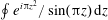


 Open access