


1. Introduction
Ocean waves transport massive amounts of energy. In terms of power per metre of wavefront, the monthly median power from wind waves above  $30\,^{\circ }\textrm {N}$ for instance, ranges from 17 to $130\ \textrm {kW}\ \textrm {m}^{-1}$ (Arinaga & Cheung Reference Arinaga and Cheung2012). Wave energy has the potential to be transformed into useful energy (Callaway Reference Callaway2007). In the case of Europe, it could be a significant contributor to the electricity supply, with an estimated 300–400 GW potential along European Atlantic coastlines alone (Babarit Reference Babarit2017). In addition to being a source of clean, renewable power, large arrays of wave energy absorbing structures may also serve the objective of mitigating coastal erosion along the shoreline (Nové-Josserand et al. Reference Nové-Josserand, Hebrero, Petit, Megill, Godoy-Diana and Thiria2018), mimicking the wave reduction effect of natural coastal defences such as mangroves, salt marshes or seagrass and kelp beds (Abanades, Greaves & Iglesias Reference Abanades, Greaves and Iglesias2015; Narayan et al. Reference Narayan, Beck, Reguero, Losada, van Wesenbeeck, Pontee, Sanchirico, Ingram, Lange and Burks-Copes2016).
Among wave energy converter concepts, oscillating wave surge converters (OWSCs), which primarily exploit the horizontal fluid motion, are identified as one of the most promising and mature technological options (Babarit Reference Babarit2017). Traditional OWSC designs consist of a rigid flap, oscillating around a rotation point, which can be fixed to the sea bed or floating (Sarkar, Renzi & Dias Reference Sarkar, Renzi and Dias2014). Recent work (Nové-Josserand Reference Nové-Josserand2018; Nové-Josserand et al. Reference Nové-Josserand, Hebrero, Petit, Megill, Godoy-Diana and Thiria2018) has investigated an artificial canopy of bio-inspired, flexible OWSCs, with the two objectives of coastline protection and energy harvesting. These arrays of flexible structures may indeed present benefits in terms of survivability and absorption capabilities, in the same way that aquatic vegetation can withstand and dissipate surface wave energy (Koehl & Wainwright Reference Koehl and Wainwright1977; Denny & Gaylord Reference Denny and Gaylord2002). From the theoretical point of view, on the one hand, each flexible element of the artificial canopy acts as an oscillator, with its intrinsic natural frequency or damping coefficient. On the other hand, the array as a whole can be viewed as a metamaterial, with properties related to its internal structure, such as the existence of crystallographic effects analogue to those observed in solid-state physics or acoustics, e.g. Bragg resonances (Garnaud & Mei Reference Garnaud and Mei2009; Arnaud et al. Reference Arnaud, Rey, Touboul, Sous, Molin and Gouaud2017; Rey et al. Reference Rey, Arnaud, Touboul and Belibassakis2018). Several studies have explored these ideas in different systems designed in view of engineering water wave propagation, ranging from the refraction phenomenon of water waves propagating through an array of bottom-mounted structures (Hu & Chan Reference Hu and Chan2005; Arnaud et al. Reference Arnaud, Rey, Touboul, Sous, Molin and Gouaud2017), to the tuning of the sea bed topography (Davies & Heathershaw Reference Davies and Heathershaw1984; Berraquero et al. Reference Berraquero, Maurel, Petitjeans and Pagneux2013), or the deployment of floating membranes with a crystalline array of defects that confer unique propagation features to the hydroelastic waves that ensue (Domino, Fermigier & Eddi Reference Domino, Fermigier and Eddi2020). Rey et al. (Reference Rey, Arnaud, Touboul and Belibassakis2018) study the propagation of water waves through dense and sparse arrays of vertical, bottom-mounted cylinders, including the reflection of oblique flume modes in the analysis. For dense arrays (where cylinder spacing in the wave direction is much smaller than the wavelength), the cylinder array is better treated as a porous medium, while Bragg reflection patterns become governed by the array length, as opposed to the cylinder spacing (Arnaud et al. Reference Arnaud, Rey, Touboul, Sous, Molin and Gouaud2017; Rey et al. Reference Rey, Arnaud, Touboul and Belibassakis2018).
In order to assess the potential, and improve the design of such flexible OWSC arrays, it is necessary to articulate individual OWSC parameters, together with the array layout, within a reasonably detailed dynamical model. Ideally, an appropriate dynamical model should be able to predict global quantities, such as the reflected, transmitted, absorbed and dissipated energy, as well as more detailed information on the dynamics of individual flexible OWSCs, such as wave loads, motion and energy absorption. The present work paves the way towards those objectives.
In the work of Nové-Josserand, Godoy-Diana & Thiria (Reference Nové-Josserand, Godoy-Diana and Thiria2019), assuming that flexible OWSCs are arranged in several rows parallel to the wavefront, a simple interaction model is proposed, which allows for assessing the effects of various parameters upon the global reflection and transmission coefficients of the array (see also Renzi & Dias (Reference Renzi and Dias2012)). Analytical formulations are derived, which relate the transmission and reflection coefficients of a single row, as well as the spacing between rows, to the transmission and reflection coefficients of the whole array. Those formulae, however, neglect successive reflections between non-neighbouring rows within the array. Furthermore, since reflection and transmission coefficients are represented as real numbers, the model does not account for the possible phase shift, induced by transmission and reflection.
In this work, building upon the ideas of Nové-Josserand et al. (Reference Nové-Josserand, Godoy-Diana and Thiria2019), an improved interaction model, similar to the one in Evans (Reference Evans1990), is proposed, which does not neglect interactions between any pair of rows, and considers complex reflection and transmission coefficients. Using the wide-spacing approximation, the proposed model is based on an iterative approach, whereby the transmission–reflection problem is solved recursively as new rows are successively added to the array. The recursion proposed in the present study determines the reflection and transmission coefficients for the concatenation of any two arrays, of which the reflection and transmission coefficients are already known. Furthermore, the obstacles are allowed to move, and absorb energy, in any combination of surge and pitch. Finally, wave dissipation within the fluid along the propagation direction is taken into account within the model.
The interaction model is validated against the results of physical experiments carried out by Nové-Josserand et al. (Reference Nové-Josserand, Godoy-Diana and Thiria2019), whereby several rows of vertical, flexible blades are subject to regular plane waves in a small-scale wave flume. Experimental results support the model accuracy.
Taking a step back from the specific problem of flexible OWSCs, the paper then focuses on the case of arrays made of identical, regularly spaced rows of obstacles. Exact formulae are retrieved for the array reflection and transmission coefficients, as functions of the properties of individual rows and array spacing, as well as asymptotic expressions when the number of rows tends to infinity. Although the derivation of those formulae does not differ, in principle, from existing work such as Linton (Reference Linton2011), in the present study the individual transmission and reflection coefficients are expressed in a formalism which emphasises the role of energy dissipation or absorption by the obstacles. As a result, the formulae obtained for the global array reflection and transmission highlight the existence of two significantly different behaviours, depending on whether or not the interaction between the wave and individual rows involves energy absorption (or dissipation).
The remainder of this paper is organised as follows. The problem and associated assumptions are defined in § 2. Section 3 presents a recursion relation to solve the reflection and transmission problem. In § 4, the predictions of the proposed model are compared with experimental results. In § 5, the special case of  $N$ identical rows is given special attention. Conclusions are provided in § 6.
2. Problem definition and assumptions
2.1. Overview of the problem
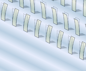
Consider an array of thin, vertical structures arranged in parallel rows, such as that illustrated in figure 1, where the extent of each row is infinite along the  $y$ axis. The water depth is assumed constant. The undisturbed incident wave is a plane wave propagating in the $x$ direction, orthogonal to the rows. The array is assumed periodic in the $y$ direction, with periodicity smaller than the wavelength; in other words, $\lambda > l+W$. Therefore, transverse modes can be neglected (Dalrymple & Martin Reference Dalrymple and Martin1990).

Figure 1. An array of wave absorbing vertical blades.
The incoming wave is described by means of the free-surface elevation (FSE),  $\eta _0$, given by the following equation:
 \begin{equation} \eta_0(x,t) = \mathrm{Re}\{\hat{\eta}_0 \exp({\textrm{i}(k x-\omega t)})\}, \end{equation}
where  $k=2{\rm \pi} /\lambda$ is the wavenumber, $\omega$ is the wave frequency and $\hat {\eta }_0$ is the complex wave amplitude. As the incoming plane wave travels through a given row, the wave–row interaction results in a transmitted plane wave and a reflected plane wave. Transmitted and reflected wave amplitudes are deduced from the incoming plane wave through transmission and reflection coefficients, respectively. Such a simple representation omits the evanescent modes, which are essential to describe the flow in the close vicinity of each row of obstacles. This implies, in particular, that the rows are sufficiently far from each other (Evans Reference Evans1990), hence the terminology ‘wide-spacing approximation’ (also known as ‘plane wave approximation’ in naval and offshore hydrodynamics). In theory, row-to-row distances greater than one wavelength are necessary for the wide-spacing approximation to be theoretically consistent (Martin Reference Martin1984), although many studies (McIver & Bennett Reference McIver and Bennett1993; chapter 6 of Linton & McIver Reference Linton and McIver2001; chapter 3 of Li Reference Li2006) find, through comparison with more accurate numerical techniques, that the wide-spacing approximation results remain accurate for distances significantly smaller than the wavelength. Also note that the wide spacing approximation does not assume that evanescent modes are non-existent: it merely assumes that they can be neglected when analysing row-to-row interaction. The wave field, as computed through the wide-spacing approximation, is only a partial description of the exact wave field, valid outside the close vicinity of the rows considered.
Finally, the interaction theory presented in this work does not assume identical rows: the obstacle characteristics, as well as their spacing, may vary across rows, but not within a given row; furthermore, the distance between consecutive rows may also vary.
2.2. Diffraction problem for a single row of fixed obstacles
First consider a single row of fixed obstacles, which constitutes a diffraction problem. For example, concerning the obstacles illustrated in figure 1, this assumption implies that the blades are infinitely rigid. The fixed row, located at a position  $x_1$, is subject to an incoming wave described as in (2.1). The wave, transmitted by the obstacle, propagates in the positive $x$ direction, and can be written as follows:
 \begin{equation} \eta_{{t}}(x,t) = \mathrm{Re}\{\hat{t} \hat{\eta}_0 \exp({\textrm{i}(kx - \omega t)})\}, \quad x>x_1. \end{equation}
The reflected wave takes the form
 \begin{equation} \eta_{{r}}(x,t) = \mathrm{Re}\{\hat{r} \hat{\eta}_0 \exp({\textrm{i}(k(2x_1-x) -\omega t)})\}, \quad x< x_1. \end{equation}
In (2.2) and (2.3),  $\hat {t}$ and $\hat {r}$ are complex-valued transmission and reflection coefficients, which apply a change in amplitude and a phase shift to the incoming wave as it reaches the obstacle position. The coefficients $\hat {t}$ and $\hat {r}$ depend on the obstacle geometry, and on the incoming wave frequency. Also note that, since the row is thin, it is considered to have a plane of symmetry transverse to the $x$ axis; therefore, the reflection coefficient is identical for incoming waves propagating in the positive and in the negative $x$ directions.
It is possible to state a few general properties which  $\hat {r}$ and $\hat {t}$ must satisfy (Linton Reference Linton2011). In linear wave theory, and considering no energy absorption or dissipation at the interface with the obstacles, preservation of energy implies that the row reflection and transmission coefficients satisfy the following equality:
 \begin{equation} |\hat{t}|^{2}+|\hat{r}|^{2} = 1. \end{equation}
 Equation (2.4) can be verified, for example, in Ursell (Reference Ursell1947), for the case where the rows of blades in figure 1 are replaced with infinitely long, submerged vertical barriers, extending along the whole  $y$ axis, or in Linton (Reference Linton2011) for the case of submerged, horizontal cylinder extending along the $y$ direction.
In the more general case, where some of the incoming wave energy can be dissipated at the interface with the obstacle, energy conservation implies the following inequality (see e.g. Isaacson, Premasiri & Yang (Reference Isaacson, Premasiri and Yang1998) for a vertical slotted barrier):
 \begin{equation} |\hat{t}|^{2}+|\hat{r}|^{2} \leq 1. \end{equation}
Note that the energy-preservation property, whether it takes the form of (2.5) or (2.4), should also be satisfied by the array as a whole.
Considering infinitely thin rows (or at least sufficiently thin with respect to the wavelength), the following relation must hold between the complex reflection and transmission coefficients  $\hat {r}$ and $\hat {t}$:
 \begin{equation} \hat{t}+\hat{r}=1. \end{equation}
Indeed, one may think of the row, excited by two incoming waves of identical amplitude, and propagating in opposite directions. The two incoming waves together form a standing wave pattern. At the antinodes of the standing waves (i.e. at the locations where the wave amplitude is the largest), the horizontal fluid velocity is zero along the whole water column. Therefore, by synchronising the two exciting waves in such a way that the obstacle is at one such antinode, the no-flow boundary conditions on the obstacle vertical boundary are naturally satisfied. The presence of the obstacle thus leaves the flow unchanged. Formulated in terms of the reflection and transmission coefficients, this is simply written as  $\hat {t}+\hat {r}= 1$. This can be verified, for example, in Huang (Reference Huang2007), for the case of porous vertical barriers, or in Ursell (Reference Ursell1947), for the case of impermeable vertical barriers covering some fraction of the distance between the surface and the sea bottom. If the assumption that the row is infinitely thin is removed, the relation $\hat {r}+\hat {t}=1$ may be replaced with $|\hat {r}+\hat {t}|=1$ (Linton Reference Linton2011), with little changes in the calculations carried out in § 5.
The properties represented by (2.6), (2.4) and (2.5) may be visualised geometrically, as shown in figures 2(a) (for a non-dissipative case) and 2(b) (in the general case). With a non-dissipative interaction,  $\hat {t}$ and $\hat {r}$ can be visualised in the complex plane as forming two sides of a right-angled triangle, of which the hypotenuse is of unitary length, as seen in figure 2(a). In contrast, a dissipative case is shown in figure 2(b). Energy preservation implies that $\hat {t}$ must lie inside the circle represented in the figure.

Figure 2. Complex transmission and reflection coefficients for a row of obstacles, (a) when no energy dissipation takes place at the interface and (b) when the interaction with the obstacle dissipates some energy.
2.3. Pitching and surging obstacles
In the foregoing section, the obstacles were considered fixed. However, pitching and surging obstacles, such as rigid or flexible OWSCs, can be modelled in the same way. Let  $\hat {r}_d$ and $\hat {t}_d$ be the reflection and transmission coefficient of an individual row, assumed fixed ( $d$ stands for diffraction). When the obstacles are oscillating, the reflected and transmitted waves are the sum of diffraction and radiation effects, the latter being the effect of the obstacle oscillating motion. Let $\hat {h}^+_{rad}$ and $\hat {h}^{-}_{rad}$ be the two coefficients such that for forced pitching or surging oscillations with complex velocity amplitude $\hat {\dot {\varTheta }}$, the wave radiated backward has amplitude $\hat {h}^{-}_{rad} \hat {\dot {\varTheta }}$, and the wave radiated forward has amplitude $\hat {h}^+_{rad}\hat {\dot {\varTheta }}$. Because of the obstacle symmetry, $\hat {h}^{-}_{rad}$ and $\hat {h}^+_{rad}$ verify that $\hat {h}^{-}_{rad} = -\hat {h}^+_{rad}$. Consider an incoming wave $\hat {\eta }_0$ propagating forward from $x = -\infty$. Let $\hat {H}^+$ denote the transfer function that relates the incoming wave to the row oscillation velocity, i.e. $\hat {\dot {\varTheta }} = \hat {H}^+\hat {\eta }_0$. Under wave excitation, the reflected wave thus has complex amplitude $(\hat {r}_d - \hat {h}^+_{rad}\hat {H}^+)\hat {\eta }_0$, while the transmitted wave has amplitude $(\hat {r}_d + \hat {h}^+_{rad}\hat {H}^+)\hat {\eta }_0$.
The reflection and transmission coefficients  $\hat {r} = \hat {r}_d - \hat {h}^+_{rad}\hat {H}^+$ and $\hat {t} = \hat {r}_d + \hat {h}^+_{rad}\hat {H}^+$ also satisfy (2.6) and (2.4) (if no energy is dissipated or absorbed by the oscillating obstacles), or (2.6) and (2.5) (if some energy is dissipated or absorbed by the oscillating obstacles).
3. A recursive numerical approach
In this section, the case of several rows is considered. As illustrated in figure 3, each row  $n$ is located at a position $x_n$ along the $x$ axis, and is characterised by its transmission and reflection coefficients, $\hat {t}_n$ and $\hat {r}_n$, respectively.

Figure 3. Wave transmission and reflection through  $N$ obstacles.
Define  $X_0, X_1,\ldots , X_N$ such that $X_0 < x_1$, $x_N < X_N$, and, for every $n$ such that $0 < n < N$, $x_{n} < X_{n} < x_{n+1}$. In the fluid domain surrounding $X_n$, and delimited by the previous and next rows, the wave field is specified by means of two coefficients $\hat {\eta }^+_n$ and $\hat {\eta }^{-}_n$, representing ‘forward’ and ‘backward’ complex wave amplitudes, such that
 \begin{equation} \eta(x,t) = \mathrm{Re}\{\hat{\eta}^+_n \exp({\textrm{i}(k(x-X_n)-\omega t)}) + \hat{\eta}^{-}_n \exp({\textrm{i}({-}k(x-X_n)-\omega t)})\}. \end{equation}
For  $n = 0$ (respectively, $n=N$), the domain where (3.1) is valid extends towards $-\infty$ (respectively, $+\infty$). Furthermore, if incoming waves propagate from $-\infty$ in the positive $x$ direction, $\hat {\eta }^+_0$ represents the forcing term of the whole system, while $\hat {\eta }^{-}_N = 0$, i.e. there is no incoming wave propagating from $+\infty$.
Consider a section  $\mathcal {S}$ of the array comprised between $X$ and $X'$, with one or more obstacles located inside the interval $[X;X']$; $\mathcal {S}$ is represented in figure 4. Define the ‘forward’ and ‘backward’ complex wave amplitudes $\hat {\eta }_+$ and $\hat {\eta }_-$ such that, in the neighbourhood of $X$, the FSE is written as follows:
 \begin{equation} \eta(x,t) = \hat{\eta}_+ \exp({\textrm{i}(k(x-X)-\omega t)}) + \hat{\eta}_- \exp({\textrm{i}({-}k(x-X)-\omega t)}). \end{equation}
Similarly, define the complex wave amplitudes  $\hat {\eta }'_+$ and $\hat {\eta }'_-$ such that, in the neighbourhood of $X'$, the FSE is written as follows:
 \begin{equation} \eta(x,t) = \hat{\eta}'_+ \exp({\textrm{i}(k(x-X')-\omega t)}) + \hat{\eta}'_- \exp({\textrm{i}({-}k(x-X')-\omega t)}). \end{equation}
Figure 4. Wave transmission and reflection through a domain  $\mathcal {S}$ (a), a domain $\mathcal {S}'$ (b) and a domain $\mathcal {S}''$ that is the combination of $\mathcal {S}$ and $\mathcal {S}'$ (c).
Assume that the reflection and transmission problems have been solved for the domain  $\mathcal {S} = [X;X']$, i.e. that complex coefficients $R_-$, $R_+$, $T_+=T_-=T$ have been found, such that, for incident wave components $\hat {\eta }_+$ and $\hat {\eta }'_-$ propagating into the domain $\mathcal {S}$, the wave components $\hat {\eta }_-$ and $\hat {\eta }'_+$, propagating away from $\mathcal {S}$, are derived as follows:
 \begin{equation} \left. \begin{gathered} \hat{\eta}_-= R_+ \hat{\eta}_++ T \hat{\eta}'_-, \\ \hat{\eta}'_+= R_- \hat{\eta}'_-+ T \hat{\eta}_+. \end{gathered} \right\} \end{equation}
In the above expression, the ‘forward’ and ‘backward’ transmission coefficients,  $T_+$ and $T_-$, are assumed identical, which will receive proper justification subsequently.
Similarly, let  $\mathcal {S}'$ be the domain comprised between $X'$ and another position $X'' > X'$, and represented in figure 4. Complex coefficients $R'_-$, $R'_+$, $T'$ have been found, such that, for incident wave components $\hat {\eta }'_+$ and $\hat {\eta }''_-$, the wave components $\hat {\eta }'_-$ and $\hat {\eta }''_+$ are determined as follows:
 \begin{equation} \left. \begin{gathered} \hat{\eta}'_-= R'_+ \hat{\eta}'_++ T' \hat{\eta}''_-, \\ \hat{\eta}''_+= R'_- \hat{\eta}''_-+ T' \hat{\eta}'_+. \end{gathered} \right\} \end{equation}
 Now define  $\mathcal {S}''$ as the domain extending from $X$ to $X''$, as represented in figure 4. By combining (3.4) and (3.5), it is straightforward to obtain a linear relation between $\{\hat {\eta }_+, \hat {\eta }''_-\}$, on the one hand, and $\{\hat {\eta }_-, \hat {\eta }''_+\}$ on the other hand, such that
 \begin{equation} \left. \begin{gathered} \hat{\eta}_-= R''_+ \hat{\eta}_++ T'' \hat{\eta}''_-, \\ \hat{\eta}''_+= R''_- \hat{\eta}''_-+ T'' \hat{\eta}_+, \end{gathered} \right\} \end{equation}
where the coefficients  $R''_+$, $R''_-$ and $T''$ are calculated as follows:
 \begin{equation} \left. \begin{gathered} R''_+=\frac{R_{-} - R'_{-}(R_+R_{-}-T^{2})}{1-R'_{-}R_+}, \\ R''_{-}=\frac{R^{'}_+ - R_+(R'_+R'_{-}-T'^{2})}{1-R'_{-}R_+},\\ T''_+= T''_-=T'' = \frac{T'T}{1-R'_{-}R_+}. \end{gathered} \right\} \end{equation}
Note that, in the above expression, if both  $\mathcal {S}$ and $\mathcal {S}'$ satisfy the condition that their forward and backward transmission coefficients are identical, the same holds for $\mathcal {S}''$.
The recursion of (3.7) can be put into practice by defining the elementary domains  $\mathcal {S}_n$ for $n = 1,\ldots , N$, only containing the $n$th row, and extending from $X_{n-1}$ to $X_{n}$. For one such domain, it is easy to find that the transmission and reflection coefficients are as follows:
 $$\begin{gather} T_n = \hat{t}_n \exp({\textrm{i} k(X_{n}-X_{n-1})}), \end{gather}$$
 $$\begin{gather}R_{n+} = \hat{r}_n \exp({2 \textrm{i} k(x_{n}-X_{n-1})}), \end{gather}$$
 $$\begin{gather}R_{n-} = \hat{r}_n \exp({2 \textrm{i} k(X_{n}-x_{n})}). \end{gather}$$
 The recursion can be initiated using the elementary domain containing the first row, thus obtaining  $T_1$, $R_1^+$ and $R_1^{-}$. Additional rows are then added sequentially through the use of (3.7). It can be seen that, for every elementary domain, the forward and backward transmission coefficients are identical, and that this property is preserved through successive iterations of (3.7), which justifies a posteriori the simplifications in (3.4) and (3.5).
The above recursion yields the global transmission and reflection coefficients of the array, denoted as  $T_{\{1,\ldots ,N\}}$, $R_{\{1,\ldots ,N\}}^+$ and $R_{\{1,\ldots ,N\}}^{-}$. For a given incident wave $\hat {\eta }^+_0$, the wave field between each pair of consecutive rows, i.e. $\hat {\eta }_n^+$ and $\hat {\eta }_n^{-}$, can be reconstructed. To that end, the reflected wave coefficient $\hat {\eta }^{-}_0$ is first calculated as $\hat {\eta }^{-}_0 = R_{\{1,\ldots ,N\}}^+ \hat {\eta }^+_0$. Then, other coefficients $\hat {\eta }^+_n$ and $\hat {\eta }^{-}_n$ for $n > 0$ are calculated recursively using the relations
 \begin{equation} \left. \begin{gathered} \hat{\eta}^+_{n} = T_n \hat{\eta}^+_{n-1} + R^{-}_n \hat{\eta}^{-}_{n},\\ \hat{\eta}^{-}_{n-1} = T_{n} \hat{\eta}^{-}_{n} + R^+_n \hat{\eta}^+_{n-1}, \end{gathered} \right\} \end{equation}
rearranged into
 \begin{equation} \left. \begin{gathered} \hat{\eta}^+_{n} = \frac{T_n^{2}-R^+_n R^{-}_n}{T_n} \hat{\eta}^+_{n-1} + \frac{R^{-}_n}{T_n}\hat{\eta}^{-}_{n-1},\\ \hat{\eta}^{-}_{n} ={-} \frac{R^+_n}{T_n} \hat{\eta}^+_{n-1} + \frac{1}{T_n}\hat{\eta}^{-}_{n-1}. \end{gathered} \right\} \end{equation}
This completes the description of the plane waves across the whole array.
In the above developments, it is assumed that, behind the last row, waves are free to propagate away from the array ( $\hat {\eta }^{-}_N = 0$). However, it can be of interest to investigate the case where waves are blocked by some reflecting structure (e.g. the coastline) behind the last row. In such a case, it is easy to simply add one more row, characterised by a transmission coefficient equal to zero, and follow the very same procedure.
An important extension of the proposed approach consists of modelling some dissipation within the fluid, by defining
 \begin{equation} \left. \begin{gathered} T_n = \hat{t}_n \exp({\textrm{i} \kappa(X_{n}-X_{n-1})}), \\ R_{n+} = \hat{r}_n \exp({2 \textrm{i} \kappa (x_{n}-X_{n-1})}), \\ R_{n-} = \hat{r}_n \exp({2 \textrm{i} \kappa (X_{n}-x_{n})}), \end{gathered} \right\} \end{equation}
with  $\kappa$ defined as $\kappa = k+\textrm {i}\nu$, where $\nu >0$ is some dissipation factor. The inclusion of such a dissipation factor is crucial in the analysis of small-scale experimental data, as reported in § 4.
It can easily be shown that, by choosing  $X_n = x_{n+1}$, the recursion of (3.12) coincides with the one proposed by Evans (Reference Evans1990). Finally, from an array optimisation perspective, the proposed ‘concatenation’ formulae of (3.7) are advantageous, since they allow the combination of arbitrary array sections.
4. Experimental validation
4.1. Experimental procedure
The proposed recursive numerical approach is validated by means of an experimental data set, recorded by Nové-Josserand et al. (Reference Nové-Josserand, Godoy-Diana and Thiria2019). The set-up consists of a small-scale wave flume (0.6 m wide, 1.8 m long), with a wave maker at one end and a sloped damping beach at the other end. The water depth is 8 cm. Flexible, vertical blades are placed in the wave flume, arranged in one, two and three rows extending along the width of the wave flume. In these experiments, the blades are surface piercing (although this is not necessary to employ the theory of §§ 2 and 3). A three-dimensional map  $\eta (x,y,t)$ of the FSE is recorded by means of an optical measurement system, as reported briefly in Appendix A, and in more detail in chapter 3 of Nové-Josserand (Reference Nové-Josserand2018). All three-dimensional mappings of the FSE are averaged along the $y$ axis, i.e. along the flume width, so that each experiment yields a signal $\eta (x,t)$. All experiments are carried out using the same excitation frequency (5 Hz), close to the blade resonant frequency (Nové-Josserand et al. Reference Nové-Josserand, Godoy-Diana and Thiria2019). A descriptive sketch of the experimental set-up is shown in figure 5.

Figure 5. Schematic diagram of the experimental set-up.
In each longitudinal position  $x$, the $\eta (x,t)$ signal is Fourier filtered at the 5 Hz excitation frequency, in order to cancel parasitic frequencies due, for example, to undesired transient events. An example of experimentally recorded signal $\eta (x,t)$ is shown in figure 6 (before and after Fourier filtering). Marked reflection patterns are visible in the up-wave zone.

Figure 6. Experimental signal  $\eta (x,t)$ for $N=2$ and $L/\lambda =0.5$, prior to Fourier filtering (a) and after Fourier filtering (b). Dotted, white lines indicate the longitudinal locations of the two rows.
The experimental validation procedure relies on the following steps.
(i) Estimate the reflection and transmission coefficients $\hat {r}$ and $\hat {t}$ of a single row of obstacles, from the results of a single-row experiment.
(ii) Estimate the reflection and transmission coefficients
$R_2, T_2, R_3, T_3$ of two- and three-row arrays, for different configurations in terms of spacing between consecutive rows.(iii) Compare
$R_2, T_2, R_3, T_3$ with their theoretical counterparts, computed using the wide-spacing recursive model proposed in § 3.


However, before the steps outlined above can be followed, several practical challenges must be overcome. First of all, because of the small size of the wave flume, wave dissipation is expected to have a significant impact on observed results. Therefore, the results of a blade-free experiment are used to calibrate the coefficient  $\nu$ of an exponential dissipation law as in (3.13). The procedure to calculate $\nu$ is reported in more detail in Appendix A.
Furthermore, the observed wavelength ( $\lambda = 6.90\ \textrm {cm}$) departs slightly from that expected from linear wave theory ( $\lambda = 6.67\ \textrm {cm}$) for capillary-gravity waves (see Appendix A). Accurate measurement of $\lambda$ was found to be highly important, especially in the process of estimating the phase of reflection and transmission coefficients. To that end, the spatial autocorrelation $a(\Delta x) = \boldsymbol {E}[\eta (x,t)\eta (x+\Delta x,t)]$ was calculated in the blade-free experiment, and $\lambda = 6.90\ \textrm {cm}$ was obtained as the distance between successive maxima of the autocorrelation function (more specifically, taking the distance between five consecutive maxima allows for excellent accuracy, below 1 %.) In addition, bearing in mind that surface tension might vary slightly across experiments, depending on impurities at the water surface, it was verified that $\lambda$ remained consistent across all four sets of experiments.
Finally, the recorded signal  $\eta (x,t)$ must be decomposed into two free wave components $\hat {\eta }_+$ and $\hat {\eta }_{-}$ propagating in the positive and negative $x$ directions, respectively. Those two components are required in order to estimate the array reflection and transmission coefficients. In this work, $\hat {\eta }_+$ and $\hat {\eta }_{-}$ are estimated based on a least squares method, thoroughly detailed in Appendix A.
4.2. Experimental results
The magnitude and phase of the transmission coefficient of a single row of flexible blades are found to be  $|\hat {t}| \approx 0.73$ and $\phi _t \approx 0.1$ rad (see in Appendix A how uncertainty in $\lambda$ and $\nu$ is accounted for in the estimate of $\hat {t}$). Note that, given those values, the row of blades is a ‘dissipating’ obstacle, since clearly $|\hat {t}|^{2} + |\hat {r}|^{2} = |\hat {t}|^{2} + |1-\hat {t}|^{2} \approx 0.61 < 1$ (see Appendix A). The missing energy is dissipated either internally (through bending) or through viscous effects.
In the set of experiments with  $N=2$ rows, the first row (i.e. the farther up-wave) is held fixed, while the spacing $L$ between both rows is gradually increased by changing the second row position; $L$ thus covers a range of discrete values, between approximately $0.25$ and one wavelength.
Figure 7 compares the reflection and transmission magnitudes obtained experimentally (crosses), with their theoretical counterparts (thick dotted and solid lines) predicted by the recursive model, including dissipation along the wave flume as in (3.13). The effect of parameter uncertainty is also visualised, by plotting the model reflection and transmission coefficients, obtained when  $|\hat {t}|$ is changed by ${\pm }5\,\%$ (thin lines, below and above the nominal results). Taking into account the significant sensitivity of the model results to the identified $\hat {t}$ magnitude, the agreement between experimental and predicted coefficients can be considered excellent, although transmission seems to be slightly overestimated by the model.

Figure 7. Reflection and transmission magnitudes as a function of  $L/\lambda$, obtained experimentally (crosses), and from the recursive theoretical model (thick lines, dotted and solid) for $N=2$ rows.
In the experimental data set with  $N=3$, the length $L_{12}$ between the first two rows is held fixed to approximately $0.25\lambda$, while $L_{23}$ is gradually increased. As evidenced by figure 8, the agreement between the model and experimental results remains satisfactory, although the model slightly underestimates reflection.

Figure 8. Reflection and transmission magnitudes as a function of  $L_{23}/\lambda$, obtained experimentally (crosses), and from the recursive theoretical model (thick lines, dotted and solid) for $N=3$ rows.
5. The particular case of identical rows
In this section, the case of identical rows is considered, whereby every row has the same transmission and reflection coefficients  $\hat {t}$ and $\hat {r}$, and the distance between each pair of consecutive rows is $L$. Indeed, in such a case, analytical formulae can be found for the array reflection and transmission coefficients (Evans Reference Evans1990; Linton Reference Linton2011). Several important results arise, regarding the effect of $L$ upon the array reflection properties, such as the existence of discrete values which completely cancel reflection, and the existence of ‘band-gaps’, i.e. intervals where reflection is high, and tends to unity as the number of rows increases. Furthermore, it has been pointed out (Linton Reference Linton2011) that, for some cases such as rows consisting of submerged, horizontal cylinders, spacing values which yield maximum reflection (i.e. the centres of the reflection band-gap intervals) are shifted with respect to the Bragg condition. In Arnaud et al. (Reference Arnaud, Rey, Touboul, Sous, Molin and Gouaud2017), which investigates a dense array of wave-dissipating vertical cylinders, treated as a porous medium, it can be noted that the Bragg-type reflection minima are not null (in contrast to cases, see e.g. Rey et al. (Reference Rey, Arnaud, Touboul and Belibassakis2018), where no dissipation is considered). In the present section, those results are revisited and clarified by adopting a formalism, which highlights the role of energy absorption or dissipation by the obstacles.
Define  $X_0 = x_1 - L/2$ and, for $n > 0$, $X_n = x_n + L/2$. For every domain $\mathcal {S}_n$, the transmission and reflection coefficients are given as
 \begin{equation} \left. \begin{gathered} T = \hat{t} \textrm{e}^{\textrm{i} k L}, \\ R^+ = R^{-} = \hat{r} \textrm{e}^{\textrm{i} k L}. \end{gathered} \right\} \end{equation}
Define
 \begin{equation} \eta_{n} = \begin{pmatrix} \hat{\eta}^+_{n} \\ \hat{\eta}^{-}_{n} \end{pmatrix}. \end{equation}
 From the recursion in (3.12),  $\eta _{n}$ and $\eta _{n+1}$ verify (Linton Reference Linton2011)
 \begin{equation} \eta_{n+1} = A \eta_{n}, \end{equation}
where the  $2\times 2$ matrix $A$ has complex entries defined as follows:
 \begin{equation} A =\frac{\textrm{e}^{-\textrm{i} k L}}{\hat{t} } \begin{pmatrix} (\hat{t}^{2}-\hat{r}^{2})\textrm{e}^{2\textrm{i} k L} & \hat{r} \textrm{e}^{\textrm{i} k L} \\ -\hat{r} \textrm{e}^{\textrm{i} k L} & 1 \end{pmatrix}. \end{equation}
 Therefore,  $\eta _0$ and $\eta _N$ are related as follows:
 \begin{equation} \eta_N = A^{N} \eta_0. \end{equation}
However, in the equation above, only  $\eta _0^+$ and $\eta _N^{-}$ are known, where $\eta _0^+$ corresponds to the system input, while $\eta _N^{-}$ is zero. Manipulating (5.5), it is easy to find the following relations:
 \begin{equation} \left. \begin{gathered} \hat{\eta}^+_N = \frac{\text{det}(A^{N})}{(A^{N})_{2,2}} \hat{\eta}^+_0, \\ \hat{\eta}^{-}_0 = \frac{-(A^{N})_{2,1}}{(A^{N})_{2,2}} \hat{\eta}^+_0. \end{gathered} \right\} \end{equation}
Therefore, the global transmission and reflection coefficients are calculated as
 \begin{equation} \left. \begin{gathered} T_N = \frac{\text{det}(A^{N})}{(A^{N})_{2,2}}, \\ R_N = \frac{-(A^{N})_{2,1}}{(A^{N})_{2,2}}, \end{gathered} \right\} \end{equation}
where  $(A^{N})_{m,n}$ denotes entry $n,m$ of the matrix $A^{N}$.
Of course, the solution above may be computed numerically. However, it is also interesting to investigate the behaviour of  $R_N$ and $T_N$ qualitatively, depending on the basic parameters $\hat {t}$, $\hat {r}$ and $L$, in order to gain more general insight. In general, any pair of coefficients $\hat {t},\hat {r}$ satisfying (2.6) may be constructed from a ‘non-dissipative’ pair of coefficients $\hat {t}',\hat {r}'$, as follows:
 \begin{equation} \left. \begin{gathered} \hat{t} = \hat{t}'-\delta, \\ \hat{r} = \hat{r}'+\delta, \end{gathered} \right\} \end{equation}
with
 \begin{equation} \delta = |\delta|\textrm{e}^{2\textrm{i}\phi}, \end{equation}
where  $|\delta | = {1}/{2}-|\hat {t}-{1}/{2}|$ and $2\phi$ is the phase of $\hat {t}-{1}/{2}$ (and $\phi$ is the phase of $\hat {t}'$). Coefficients $\hat {t}$, $\hat {r}$, $\hat {t}'$, $\hat {r}'$, $\delta$ are illustrated in figure 9. Essentially, $\hat {t}'$ is the transmission coefficient which is the closest to $\hat {t}$, while representing a non-dissipative obstacle. It is easy to show that $\hat {t}'$ and $\hat {r}'$ verify
 \begin{equation} \left. \begin{gathered} \hat{t}' = \cos\phi \textrm{e}^{\textrm{i}\phi}, \\ \hat{r}' ={-}\textrm{i}\sin\phi \textrm{e}^{\textrm{i}\phi}. \end{gathered} \right\} \end{equation}
Figure 9. Graphical representation in the complex plane of the transmission and reflection coefficients  $\hat {t}$ and $\hat {r}$ in terms of the ‘non-dissipative’ coefficients $\hat {t}'$ and $\hat {r}'$.
With the decomposition of (5.8), the entries of  $A$ may be rewritten as a function of $L$,
$L$,  $|\delta |$ and $\phi$, using the following equations:
 \begin{equation} \left. \begin{gathered} \hat{t}^{2}-\hat{r}^{2}= \hat{t}-\hat{r} = (1-2|\delta|)\textrm{e}^{2\textrm{i}\phi} ,\\ \hat{t} = \hat{t}'-\delta = (\cos \phi - |\delta|\textrm{e}^{\textrm{i}\phi})\textrm{e}^{\textrm{i}\phi} ,\\ \hat{r} = \hat{r}'+\delta = ({-}i\sin \phi + |\delta|\textrm{e}^{\textrm{i}\phi})\textrm{e}^{\textrm{i}\phi}. \end{gathered} \right\} \end{equation}
 Define, for  $\psi \in [0;2{\rm \pi} [$,
 \begin{equation} \left. \begin{gathered} f(\psi) = \cos \psi - |\delta| \textrm{e}^{\textrm{i}\psi}, \\ g(\psi) = |\delta| \textrm{e}^{\textrm{i}\psi} - \textrm{i} \sin \psi, \end{gathered} \right\} \end{equation}
as well as the new variable  $\theta = k L+\phi$.
The matrix  $A$ may now be reformulated as follows:
 \begin{equation} A =\frac{1}{f(\phi)} \begin{pmatrix} (1-2|\delta|)\textrm{e}^{\textrm{i}\theta} & g(\phi) \\ -g(\phi) & \textrm{e}^{-\textrm{i}\theta} \end{pmatrix}. \end{equation}
 In order to obtain an analytical solution for the global transmission and reflection coefficients,  $A^{N}$ should be calculated explicitly as a function of the model parameters. Instead of the recursion in Evans (Reference Evans1990), we can also proceed through a diagonalisation of $A$, or use the direct result proposed by Williams (Reference Williams1992) for powers of $2\times 2$ matrices. Let $\rho _1$ and $\rho _2$ be the two eigenvalues of $A$. Then
 \begin{equation} A^{N}=\begin{cases} \dfrac{\rho_1^{N}}{\rho_1-\rho_2}(A-\rho_2 I_2) - \dfrac{\rho_2^{N}}{\rho_1-\rho_2}(A-\rho_1 I_2) & \text{if } \rho_1 \neq \rho_2,\\ \rho_1^{N-1}(NA-(N-1)I_2) & \text{if } \rho_1 = \rho_2. \end{cases} \end{equation}
 The two eigenvalues of  $A$ are found to be
 \begin{equation} \left. \begin{gathered} \rho_1 = \frac{f(\theta)}{f(\phi)} + \left(\frac{f(\theta)^{2}}{f(\phi)^{2}}-1\right)^{{1}/{2}},\\ \rho_2 = \frac{f(\theta)}{f(\phi)} - \left(\frac{f(\theta)^{2}}{f(\phi)^{2}}-1\right)^{{1}/{2}}. \end{gathered} \right\} \end{equation}
It is easily verified that  $\rho _1 \rho _2 = 1$. Adopting the same idea as Evans (Reference Evans1990), define $\alpha \in \mathbb {C}$ such that $\cosh (\alpha )={f(\theta )}/{f(\phi )}$, and $\beta \in \mathbb {C}$ such that $\cosh (\beta )={g(\theta )}/{g(\phi )}$. Then, $\rho _1 = \textrm {e}^{\alpha }$ and $\rho _2 = \textrm {e}^{-\alpha }$. Using (5.14), we finally use the fact that $f(\phi )\sinh (\alpha )=g(\phi )\sinh (\beta )$ to obtain relatively simple expressions (Evans Reference Evans1990) for $R_N$ and $T_N$ as follows:
 \begin{equation} \left. \begin{gathered} R_N = \frac{\sinh(N\alpha)}{\sinh(N\alpha + \beta)},\\ T_N = \frac{\sinh(\beta)}{\sinh(N\alpha + \beta)}. \end{gathered} \right\} \end{equation}
 Noting that  $f(\theta +{\rm \pi} )/f(\phi ) = -f(\theta )/f(\phi )$ and $g(\theta +{\rm \pi} )/g(\phi ) = -g(\theta )/g(\phi )$, it is easy to see that $\alpha (\theta +{\rm \pi} ) = \alpha (\theta )+\textrm {i}{\rm \pi}$ and $\beta (\theta +{\rm \pi} ) = \beta (\theta )+\textrm {i}{\rm \pi}$. Hence, $R_N(\theta +{\rm \pi} ) = -R_N(\theta )$ and $T_N(\theta +{\rm \pi} ) = (-1)^{N} T_N(\theta )$. As far as the reflection and transmission magnitudes are concerned, it is thus sufficient to study $R_N$ and $T_N$ on any interval of length ${\rm \pi}$.
5.1. Non-dissipative obstacles
In the particular case of non-dissipative obstacles, i.e. obstacles verifying  $|\hat {r}|^{2}+|\hat {t}|^{2}=1$, the parameter $|\delta |$ is zero, so that the functions $f(\theta )/f(\phi )$ and $g(\theta )/g(\phi )$ reduce to $\cos \theta /\cos \phi$ and $\sin \theta /\sin \phi$, respectively.
First consider  $\theta$ in the interval $]-\phi ; \phi [$. Then $\cos \theta / \cos \phi$ is a real number greater than unity, so that $\alpha$ is a real number, which increases from $0$ to ${\textrm {acosh}} (1/ \cos \phi )$ for $\theta = [-\phi ;0]$, and decreases from ${\textrm {acosh}} (1/ \cos \phi )$ to $0$ for $\theta \in [0; \phi ]$. Over the same interval, $\beta$ is an imaginary number which goes from $i {\rm \pi}$ to $0$, with $\beta = \textrm {i}{\rm \pi} /2$ for $\theta = 0$. Noting $\alpha = a$ and $\beta = \textrm {i} b$, $a$ and $b$ verify $a = {\textrm {acosh}}(\cos \theta /\cos \phi )$ and $b = {\textrm {acosh}}(\sin \theta /\sin \phi )$. Here $R_N$ can be written as
 \begin{equation} R_N = \frac{\sinh(N a)}{\sinh(N a + \textrm{i} b)}, \end{equation} $|R_N|$ has no roots over $]-\phi ; \phi [$ and reaches its maximum value for $\theta = 0$,
 \begin{equation} |R_N|_{max} = \frac{1-\left(\dfrac{1-\sin\phi}{1+\sin\phi}\right)^{N}}{1+\left(\dfrac{1-\sin\phi}{1+\sin\phi}\right)^{N}}. \end{equation}
As  $\theta$ approaches the bounds of the interval, $-\phi$ and $\phi$, both the numerator and the denominator of $R_N$ tend to zero. A tedious first-order development yields the following value for $|R_N|$ for $\theta = n{\rm \pi} \pm \phi$:
 \begin{equation} |R_N|_{\theta = n{\rm \pi} \pm \phi} = \frac{N}{\sqrt{N^{2}+\cot^{2}\phi}}. \end{equation}
 The interval  $\theta \in ]-\phi ; \phi [$ corresponds to $2{\rm \pi} L/\lambda \in ]-2\phi ; 0[$. It is the ‘band-gap’ interval in Linton (Reference Linton2011) and Evans (Reference Evans1990), where reflection is high, and tends to unity as $N$ grows to infinity.
Outside the band-gap interval, i.e.  $\theta \in ]\phi ;{\rm \pi} -\phi [$, $\alpha = \textrm {i} a$ where $a$ is real and increases in $]0;{\rm \pi} [$. Meanwhile, $\beta = b$ where $b$ is real, and $\beta ({\rm \pi} -\theta ) = - \beta (\theta )$. Therefore, the numerator of $R_N$ is $i\sin Na$, which cancels exactly $N-1$ times over $]\phi ;{\rm \pi} -\phi [$, while the denominator is strictly non-zero. Those are the well known discrete values of $L/\lambda$ which completely cancel reflection. Furthermore, $|R_N|$ is bounded from above as follows:
 \begin{equation} |R_N| \leq \sin\phi/\sin\theta \end{equation}
with equality when  $Na \equiv ({{\rm \pi} }/{2}) [{\rm \pi} ]$, which occurs $N$ times over the interval $]\phi ; {\rm \pi}-\phi [$.
For two representative choices of parameters  $\hat {t}$ and $\hat {r}$, numerical examples of $|R_N|$ are provided in figure 10, for $N = 2, 3, 4, 5$ and $10$. In the top graphs ( $\phi = {\rm \pi}/8$), individual rows predominantly transmit incident waves while, in the bottom graphs, individual rows predominantly reflect incident waves ( $\phi = 3{\rm \pi} /8$). Those two parameter options are illustrated in figure 10(f,l).

Figure 10. Reflection coefficient magnitude for a set of  $N$ equally spaced rows of obstacles with no energy dissipation ( $|\delta | = 0$), with $N = 2, 3, 4, 5, 10$ (a–e,g–k), for $\phi = {\rm \pi}/8$ (‘transmission-dominated’) and $\phi = 3{\rm \pi} /8$ (‘reflection-dominated’). The two parameter options for $\hat {r},\hat {t}$ of individual rows are represented in panels (f,l). See also figure 9 for the meaning of $\phi$ and $|\delta |$.
The mathematical characterisation of  $|R_N|$ can be appreciated in the different graphs of figure 10 as follows.
(i) In the interval
$[n {\rm \pi}+\phi ; (n+1){\rm \pi} -\phi ]$, delimited by means of vertical, dashed lines, there are $N-1$ values of $\theta$ which completely cancel reflection, as expected. Here $|R_N|$ oscillates between $0$ and the envelope function $\sin \phi /\sin \theta$ (dashed lines).(ii) In the interval
$[n {\rm \pi}-\phi ; n{\rm \pi} +\phi ]$, $|R_N|$ remains larger than ${N}/{\sqrt {N^{2}+\cot ^{2}\phi }}$, which is reached for $n{\rm \pi} \pm \phi$ (indicated by rounded markers).


It is interesting to see that maximum reflection is obtained for  $\theta$ within intervals of the form $[n{\rm \pi} -\phi ;n{\rm \pi} +\phi ]$, which corresponds to $kL \in [n{\rm \pi} -2\phi ;n{\rm \pi} ]$. Those intervals are wider as $\phi$ increases, i.e. as the reflection coefficient of individual rows predominates over their transmission coefficient. Furthermore, as $N$ increases, reflection tends to unity over the whole band-gap width, while it remains bounded from above by the function $\sin \phi /\sin \theta$ outside band-gap intervals. Finally, band-gaps are centred around $kL = n{\rm \pi} -\phi$, which is in contrast to ‘classical’ Bragg peaks which occur for $kL = n{\rm \pi}$, as pointed out by Linton (Reference Linton2011). Therefore, strictly speaking, those two conditions only coincide if the phase of the transmission coefficient is small. However, given the location of the band-gap interval as specified above, the Bragg condition $kL = n{\rm \pi}$ is never outside, but always at the limit of the band-gap interval (even for large $\phi$).
5.2. Dissipative obstacles
The case where dissipation occurs is more complicated, since the parameter  $|\delta |$ is now different from zero. However, it is easy to find the asymptotic behaviour of $R_N$ and $T_N$ as $N$ tends to infinity: while $T_N$ tends to zero, $R_N$ tends to $R_{\infty } =\textrm {e}^{-\beta }$.
The behaviour of  $|R_N|$ is illustrated in figure 11 for $N = 2, 3, 4, 5, 10$ as well as $|R_{\infty }|$, for ‘transmission dominated’ cases (panels (a–g)) and ‘reflection dominated’ cases (panels (h–n)). In both sets of graphs, two different values of $|\delta |$ are shown: $|\delta | = 0.1$ (weak dissipation, lighter colour) and $|\delta | = 0.4$ (strong dissipation, darker colour). As can be seen in figure 11, $|R_N|$ oscillates around $|R_{\infty }|$. There is a larger number of oscillations as $N$ increases, and oscillations are less marked as $|\delta |$ approaches its maximum possible value of $0.5$. The figure also suggests that, even for relatively small $N$, the asymptotic function $|R_{\infty }|$ is an acceptable approximation for $|R_{N}|$.

Figure 11. Transmission coefficient magnitude for a set of  $N$ equally spaced rows, with $N = 2, 3, 4, 5, 10$ and $N\rightarrow \infty$, and four parameter options regarding $\phi$ and $|\delta |$. In each graph, the lighter and darker lines correspond, respectively, to $|\delta | = 0.1$ (weak energy absorption or dissipation) and $|\delta | = 0.4$ (strong energy absorption or dissipation). The panels (a–f) and (h–m) are for ‘transmission-dominated’ and ‘reflection-dominated’ interactions, respectively. The four parameter options are represented in panels (g,n). See also figure 9 for the meaning of $\phi$ and $|\delta |$.
This time, there are no values of  $\theta$, for which $|R_N|$ vanishes. It is interesting to see that a similar result is obtained in the case of an array of cylinders, as studied by Arnaud et al. (Reference Arnaud, Rey, Touboul, Sous, Molin and Gouaud2017). Therefore, it seems to hold rather generally that, in the case of obstacle arrays made of identical rows, the presence of absorption or dissipation by individual rows makes it impossible to obtain zero reflection. One of the consequences is in terms of wave energy absorption: absorbing the totality of the incoming wave energy would imply cancelling both reflection and transmission coefficients. Therefore, total absorption of the incoming wave energy is impossible with an array of identical rows.
In the non-dissipative scenarios previously studied, the transmitted wave amplitude  $|T_N|$ could simply be calculated using the fact that $|T_N|^{2}+|R_N|^{2}=1$. In the present case, some part of the wave energy is dissipated or absorbed by the obstacles, so that $|T_N|$ cannot be immediately deduced from $|R_N|$. Therefore, it is interesting, for the sake of completeness, to also illustrate $|T_N|$; figure 12 shows $|T_N|$ for the same range of cases as figure 11 (except for $N\rightarrow \infty$ since $T_{\infty }$ is simply zero). As can be appreciated in the figure, $|T_N|$ also exhibits some oscillatory behaviour. Unsurprisingly, $|T_N|$ fades out to zero more rapidly for stronger dissipation (larger $|\delta |$), and when reflection of individual rows is larger than their transmission.

Figure 12. Transmission coefficient magnitude for a set of  $N$ equally spaced rows, with $N = 2, 3, 4, 5, 10$, and four parameter options regarding $\phi$ and $|\delta |$. In each graph, the lighter and darker lines correspond, respectively, to $|\delta | = 0.1$ (weak energy absorption or dissipation) and $|\delta | = 0.4$ (strong energy absorption or dissipation). The panels (a–e) and (g–k) are for ‘transmission-dominated’ and ‘reflection-dominated’ interactions, respectively. The four parameter options are represented in panels (f,l). See also figure 9 for the meaning of $\phi$ and $|\delta |$.
The asymptotic function  $|R_{\infty }|$ deserves particular attention. To that end, figure 13 shows $|R_{\infty }|$ for a wide range of possible scenarios regarding $\phi$ and $|\delta |$ (illustrated in the circles on both sides of the figure). As can be appreciated in figure 13, for $|\delta |>0$, the asymptotic function $|R_\infty |$ shows a marked peak, reaching unity for distances $L$ such that $kL = n{\rm \pi}$. This corresponds to classical Bragg peaks. Unsurprisingly, the peak width is smaller for larger $|\delta |$ (i.e. individual rows tend to dissipate more energy) and for obstacles for which transmission is predominant. It is also interesting to note that, even for relatively small (but non-zero) $|\delta |$ values, a strong contrast can be observed with respect to the band-gaps associated with ‘non-dissipative’ obstacles.

Figure 13. Asymptotic reflection magnitude  $|R_{\infty }|$ for different values for $\phi$, and from $|\delta | = 0$ (non-dissipative case, lightest colour) to $|\delta | = 1/2$ (darkest colour). The corresponding $\hat {t}$ and $\hat {r}$ coefficients can be visualised in the circles on both sides.
We now briefly turn back to the problem of wave energy absorption. Given that  $T_{\infty } = 0$, the energy absorbed by the whole array is proportional to $1-|R_{\infty }|^{2}$, and thus larger for smaller $|R_{\infty }|$. Figure 13 allows the visualisation of those $\hat {r}, \hat {t}$ parameters, which are more favourable from an energy absorption perspective. It appears that stronger transmission by individual rows (e.g. the top-left graph) is desirable, so that $\hat {t}$ should be chosen close to unity; with such parameters, the array absorbs most of the incoming wave energy, if the inter-row spacing does not match the Bragg condition. However, the particular case $\hat {t}=1, \hat {r} = 0$ merely corresponds to an absence of obstacles (and hence yields no energy absorption at all).
Finally, the limiting case  $|\delta | = 0.5$ (i.e. $\hat {t} = \hat {r} = 0.5$) corresponds to the reflection/transmission characteristics of a single row of wave energy devices operating under optimal power-maximising control (Evans Reference Evans1981). Nevertheless, as evidenced by the top-left graph, the choice $|\delta | = 0.5$ is suboptimal for power absorption by the array as a whole. In other words, parameter tuning may be optimal for individual rows, but suboptimal for the interacting array. The need for model-based optimisation, articulating individual row parameters together with array interaction, is thus confirmed.
6. Conclusion
With a view to the modelling and optimisation of wave energy farms, a simple recursive formulation has been employed, based on the wide-spacing approximation, to solve for the transmission and reflection of plane water waves through a number of rows of thin, vertical obstacles, where each row is characterised by complex reflection and transmission coefficients. The method allows the combination of any pair of adjacent subdomains of the fluid, for which the reflection and transmission coefficients have already been solved, thus lending itself to efficient numerical solution. Additional effects, such as linear dissipation along a wave flume, or partial reflection by the shore or an absorption beach, may be easily incorporated in the analysis. The theoretical limitations of the model, in terms of applicability, are related to the array periodicity in the direction, transverse to the incoming wave direction, which must be smaller than the wavelength, and to the distance between consecutive rows, which must not be too small relative to the wavelength.
The array reflection and transmission, predicted by the recursive model from the reflection and transmission coefficients of individual rows, are compared with the results of small-scale physical experiments comprising  $N=2$ and $N=3$ rows of vertical, flexible blades. There is a close agreement between experimental and theoretical results, even though the distance between consecutive rows is at times significantly smaller than the wavelength, which corroborates the results of several numerical studies (McIver & Bennett Reference McIver and Bennett1993; chapter 6 of Linton & McIver Reference Linton and McIver2001; chapter 3 of Li Reference Li2006), as well as experimental results (e.g. Liu, Li & Zhu (Reference Liu, Li and Zhu2016), dealing with submerged semicircular bars). Those conclusions suggest that the approach can be considered a suitable modelling option for further simulation and optimisation of OWSCs.
In the case of identical, regularly spaced rows, distinctive behaviours are identified, depending on whether individual rows predominantly reflect or transmit waves, and whether or not they dissipate energy. With no dissipation, the well known fact that discrete values of the row-to-row distance  $L$ cancel reflection is retrieved and clarified. In each interval of width $\lambda /2$, where $\lambda$ is the wavelength, there are exactly $N-1$ values of $L$ which cancel reflection, and those values are all located within an interval, with width governed by the reflection/transmission balance of individual rows. The existence of band-gap intervals is also retrieved, centred away from the classical Bragg resonant condition. In contrast, when dissipation is present, the reflection magnitude $|R_N|$ is always non-zero and, as $L$ grows, oscillates close to a reasonably simple asymptotic function $R_{\infty }$, which is interesting to investigate. In contrast to the non-dissipative case, reflection maxima take the form of the well known Bragg peaks, reaching unity when $L$ is a multiple of $\lambda /2$. Such peaks are narrower as more dissipation takes place. Finally, from the point of view of power absorption, results illustrate the fact that design parameters may be optimal for individual rows, but suboptimal as soon as array interaction is considered, thus confirming the need for joint optimisation of device and array characteristics.
Regarding the objective of wave energy farm modelling and optimisation, further work is still required towards a sufficiently detailed mathematical model of flexible OWSC farms. In particular, it should be noted that reflection and transmission coefficients of individual rows are determined by both the obstacle geometry, and by their dynamical behaviour, including the possible use of control. Array optimisation of flexible OWSCs will require the distinct articulation of geometry and control effects, since those may have significantly different implications in terms of investment cost.
In addition, ocean waves are best described as Gaussian, random processes (Pierson Reference Pierson1952), as opposed to the monochromatic case treated in the present study. Such random waves are statistically characterised by their spectral density function, which shows how energy is distributed across frequencies. It will be interesting to assess how the array affects the wave field energy content, both up-wave and down-wave – the latter being particularly important for coastal protection purposes. To that end, the methodology employed in this paper can be readily generalised to polychromatic (random) wave excitation signals. It is sufficient to know the reflection and transmission coefficients of individual rows of obstacles over a range of frequencies covering the incident wave spectrum bandwidth. The array reflection and transmission coefficients then become complex functions of the frequency, and every variable of interest (reflected or transmitted spectrum, absorbed power, obstacle motions, and so on) can be analysed in terms of dynamical systems driven by Gaussian inputs. In particular, the tuning of row-to-row spacing and other design parameters will need to be chosen, taking into account typical wave spectra at the location considered, not just one frequency.
Acknowledgements
The authors would also like to thank C. Nové-Josserand, for making her experimental data set available to us.
Funding
This project has received funding from the European Union's Horizon 2020 research and innovation programme under the Marie Skłodowska-Curie grant agreement no. 842967.
Declaration of interests
The authors report no conflict of interest.
Appendix A. Experimental data processing
A.1. Experimental set-up
The experiments were run in a small-scale (1/1000) wave flume at Laboratoire de Physique et Mécanique des Milieux Hétérogènes, associated with a two-dimensional surface wave measurement technique. The tank is 0.6 m wide and 1.8 m long. A three-dimensional map ( $x$,
$x$,  $y$,
$y$,  $t$) of the FSE is obtained through the synthetic schlieren technique (Moisy, Rabaud & Salsac Reference Moisy, Rabaud and Salsac2009), of which the working principle is as follows. The experiment is filmed from above by means of a high-speed camera. The tank bottom is covered with a random dotted pattern, over which the waves act as a magnifying glass as they propagate along the flume. Each recorded frame is compared with a reference image, taken with a still water surface, by means of statistical correlation analysis, thus providing a deformation map of the water surface, first converted into a surface gradient, which is then numerically integrated to obtain the FSE. The procedure is covered in more detail in chapter 3 of Nové-Josserand (Reference Nové-Josserand2018).
The flexible blades are made of Mylar sheets of thickness  $350\ \mathrm {\mu }\textrm {m}$, width 14 mm and length 9 cm (1 cm more than the water depth). The blades are fixed to the flume bottom by means of a Lego base, which allows for placing the blades in various configurations.
The possible influence of waves being reflected by the flume damping beach is avoided, by limiting the analysis time window below the time necessary for waves to travel from the wave maker to the beach, and back to the observation zone where the blade array is located. Similarly, the analysis time window starts sufficiently late so that transient dynamics have faded out. In this work, the analysis time window of each experiment has a duration of 2 s, which covers 10 wave periods. The spatial zone of analysis, illustrated in figure 6, is restricted to a 40 cm long area, encompassing the Lego base.
Finally, the  $\eta (x,y,t)$ mapping is averaged along the $y$ direction, thus obtaining a two-dimensional $\eta (x,t)$ mapping, as illustrated in figure 6. Here $\eta (x,t)$ is Fourier-filtered at the 5 Hz excitation frequency, to obtain a single position-dependent complex amplitude coefficient $\hat {\eta }(x)$, which characterises the wave field.
A.2. Wavenumber and dissipation coefficient estimation
For waves at a 5 Hz frequency, surface tension effects are not negligible anymore, so that the theoretical dispersion relation should follow that of capillary-gravity waves,
 \begin{equation} \left(g k + \frac{\sigma}{\rho} k^{3}\right)\tanh(kh)=\omega^{2}, \end{equation}
where  $\sigma = 0.074\ \textrm {N}\ \textrm {m}^{-1}$ and $\rho = 1000\ \textrm {kg}\ \textrm {m}^{-3}$ are the water surface tension and density, respectively. As mentioned in § 4, the observed wavelength ( $\lambda = 6.90\ \textrm {cm}$) departs slightly from that expected from the above theoretical relation ( $\lambda = 6.67\ \textrm {cm}$). Such a difference may be attributed to imperfect cleanliness of the water surface, which may have increased the surface tension value. Alternatively, the deviation may have been due to the presence of a relatively slow Stokes-induced current (less than $1\ \textrm {cm}\ \textrm {s}^{-1}$), which would have resulted in a Doppler effect. Those possibilities are the subject of ongoing investigation by the authors.
A blade-free experiment is used to estimate the wave flume dissipation coefficient, following (3.13). In the absence of perturbation of the generated wave field, for any two longitudinal positions  $x_1$, $x_2$, $\hat {\eta }$ satisfies $\hat {\eta }(x_2) = \exp ({\textrm {i} \kappa (x_2-x_1)}) \hat {\eta }(x_1)$, with $\kappa = k + \textrm {i} \nu$. Therefore, the wave amplitude $|\hat {\eta }|$ decreases as $\textrm {e}^{-\nu x}$.
Here  $|\hat {\eta }(x)|$ is smoothed using a moving average filter, thus yielding the blue curve in figure 14 (shown in logarithmic scale). The best fit is found for a dissipation rate $\nu = 2.15\ \text {m}^{-1}$, also shown in figure 14, along with the corresponding lines obtained when $\nu$ is changed by ${\pm }5\,\%$. Note that the assumption of a homogeneous dissipation coefficient along the wave flume is somewhat a simplification. In fact, the figure suggests that dissipation might be stronger in the central area (15–25 cm into the analysis zone), where the Lego base is located.

Figure 14. Dissipation coefficient identification.
In all subsequent experiments, with blades in the small-scale flume, the equivalent wavenumber is considered to be  $\kappa = 2{\rm \pi} /\lambda + \textrm {i} \nu$, where $\lambda$ and $\nu$ are the measured wavelength and dissipation rate.
A.3. Transmission and reflection coefficient estimation
The experimental identification of an array's reflection and transmission coefficients requires the separation of the forward- and backward-propagating wave amplitudes in a given observation zone, which is not a simple matter. In this work, a least squares method is employed, based on the idea introduced by Mansard & Funke (Reference Mansard and Funke1980).
Let  $x_1,\ldots ,x_M, M >2$ be a set of longitudinal positions in the up-wave zone of the flume (i.e. between the wave maker and the blade array), and let $x_0$ be a reference position. The complex wave amplitudes $\hat {\eta }(x_1), \hat {\eta }(x_2) ,\ldots ,\hat {\eta }(x_M)$ are measured. The total wave in the zone is the sum of a forward-propagating wave $\hat {\eta }_+$ and a backward-propagating wave $\hat {\eta }_-$, such that in every position $x_m$, $\hat {\eta }(x_m) = \exp ({\textrm {i}\kappa (x_m-x_0)})\hat {\eta }_+ + \exp ({-\textrm {i}\kappa (x_m-x_0)})\hat {\eta }_-$. Define
 \begin{align} \boldsymbol{z} = \begin{pmatrix} \hat{\eta}(x_1) \\ \hat{\eta}(x_2) \\ \vdots \\ \hat{\eta}(x_M) \end{pmatrix} ,\quad \boldsymbol{y} = \begin{pmatrix} \hat{\eta}_+ \\ \hat{\eta}_- \end{pmatrix}, \quad \boldsymbol{A} = \begin{pmatrix} \exp({\textrm{i}\kappa (x_1-x_0)}) & \exp({-\textrm{i}\kappa (x_1-x_0)}) \\ \exp({\textrm{i}\kappa (x_2-x_0)}) & \exp({-\textrm{i}\kappa (x_2-x_0)}) \\ \vdots & \vdots \\ \exp({\textrm{i}\kappa (x_M-x_0)}) & \exp({-\textrm{i}\kappa (x_M-x_0)}) \\ \end{pmatrix}. \end{align}
 Finding  $\hat {\eta }_+$ and $\hat {\eta }_-$ is achieved by solving the equation $\boldsymbol {A}\boldsymbol {y} = \boldsymbol {z}$ in a least-square error sense, i.e.
 \begin{equation} \tilde{\boldsymbol{y}}=(\boldsymbol{A^{*}A})^{{-}1}\boldsymbol{A^{*}}\boldsymbol{z}, \end{equation}
where  $^{*}$ denotes conjugate transpose.
The same method is applied in the down-wave zone with a set  $x'_1,\ldots ,x'_M$ of down-wave positions and a reference position $x'_0$, to obtain $\hat {\eta }'_+$ and $\hat {\eta }'_-$, the forward and backward wave coefficients in the down-wave zone. As pointed out by Mansard & Funke (Reference Mansard and Funke1980), this procedure exhibits some sensitivity to the choice of measurement points $x_m$ and $x'_m$, but less so than by using only two measurement points and proceeding through a direct inversion of a $2 \times 2$ system.
Once forward and backward wave amplitudes have been estimated in the up-wave and down-wave zones, the reflection and transmission coefficients of any array located between positions  $x_0$ and $x'_0$ can be calculated as follows:
 \begin{equation} \left. \begin{gathered} \hat{R}=\hat{\eta}_-{/}\hat{\eta}_+ ,\\ \hat{T}=\hat{\eta}'_+{/}\hat{\eta}_+. \end{gathered} \right\} \end{equation}
 However, as mentioned above, results are sensitive to the choice of measurement points  $x_1,\ldots ,x_M$ and $x'_1,\ldots ,x'_M$. Therefore, similarly to the procedure followed by Nové-Josserand et al. (Reference Nové-Josserand, Godoy-Diana and Thiria2019), a set of 30 positions $x_1,\ldots ,x_{M = 30}$ is randomly selected in the up-wave interval, as well as in the down-wave interval, and $\hat {R}$ and $\hat {T}$ are estimated based on those two sets of random points. The same procedure is iterated 100 times (i.e. with 100 different choices of 30 random locations), and the average $\hat {R}$ and $\hat {T}$ coefficients are taken as the final estimates. The up-wave interval is between 0 and 100 mm inside the frame, while the down-wave interval is between 250 and 350 mm inside the frame.
The identification of  $\hat {r}$ and $\hat {t}$ for a single row is of particular importance. This was done by employing the procedure outlined above, and choosing both $x_0$ and $x'_0$ equal to the row position. The results of the identification procedure are illustrated in figure 15, where the 100 different pairs of coefficients are shown in the complex plane as small markers, along with their average as larger, circular markers. It can be seen that the sum of the estimated $\hat {t}$ and $\hat {r}$ identified is reasonably close to unity, as expected from (2.6) (see also figure 2).

Figure 15. Estimated reflection and transmission coefficients for a single row of blades, as well as their sum.
However, the phase of  $\hat {t}$ is found to exhibit high sensitivity to the exact wavelength estimate $\lambda$, while that of $\hat {r}$ depends strongly on the exact referencing of the row position in the recorded frame $x_0$. In contrast, the norm of both coefficient estimates is almost insensitive to those parameters. Therefore, it is preferable to confirm the estimates above through the use of an alternative method. This is done by estimating only $|\hat {r}|$ and $|\hat {t}|$ (which are almost insensitive to $\lambda$ and $x_0$), using the approach outlined above, and using the fact that $\hat {r} + \hat {t} = 1$. More specifically, in each random choice of $M=30$ random points up-wave and down-wave, the norms $|\hat {r}|$ and $|\hat {t}|$ are calculated by taking the norm of (A3). The procedure is iterated 100 times, which yields reliable estimates of $|\hat {r}|$ and $|\hat {t}|$. Finally, using $\hat {r} + \hat {t} = 1$, it is found that
 \begin{equation} \phi_{t} ={\pm} {\textrm{acos}}\left(\frac{1+|\hat{t}|^{2}-|\hat{r}|^{2}}{2|\hat{t}|}\right). \end{equation}
 Among the two possible values for the phase of  $\hat {t}$, the negative one is more consistent with the observations in figure 15, and is therefore chosen. The resulting estimate $\hat {t}$ is indicated by means of a square in figure 15, very close to the one obtained through the direct estimate (average of the green crosses in figure 15).
Finally, it is worth noting that the row of blades is a ‘dissipative’ obstacle, since clearly  $|\hat {t}|^{2} + |\hat {r}|^{2} < 1$ (in other words, $\hat {t}$ and $\hat {r}$ are not located on the circle pictured in the figure). The energy dissipation splits into external dissipation (through friction and drag) and internal dissipation (through the blade internal damping). Only the latter may be converted into useful energy. However, in this work, we do not investigate the balance between external and internal dissipation.


 Open access