


1. Introduction
With the significant advances in experimental techniques and high-performance computation in recent years, there has been overwhelming evidence indicating the existence of large-scale structures away from the wall in wall turbulence (see, for example, Smits, McKeon & Marusic (Reference Smits, McKeon and Marusic2011), and the references therein), and it has been observed that influences from the large-scale outer structure affect the magnitude of small-scale events in the near-wall region (e.g. Hutchins & Marusic Reference Hutchins and Marusic2007; Dogan et al. Reference Dogan, Örlü, Gatti, Vinuesa and Schlatter2019). Such a top-down effect from the outer to the inner structure is often referred to as ‘amplitude modulation’, and the degree of the modulation has been reported to be increasingly significant at higher Reynolds numbers (e.g. Mathis, Hutchins & Marusic Reference Mathis, Hutchins and Marusic2009). Recent experimental data from high-Reynolds-number facilities such as the Princeton Superpipe (Hultmark et al. Reference Hultmark, Vallikivi, Bailey and Smits2012) and the CICLoPE at the University of Bologna (Willert et al. Reference Willert, Soria, Stanislas, Klinner, Amil, Eisfelder, Cuvier, Bellani, Fiorini and Talamell2017; Samie et al. Reference Samie, Marusic, Hutchins, Fu, Fan, Hultmark and Smits2018) have clearly shown emergence of the outer peak of the streamwise velocity fluctuation at very high Reynolds numbers, indicating that the large-scale structures may play further important roles at higher Reynolds numbers, including interfering with the near-wall structures. These observations have raised interest in energy transfer caused by interactions between different scales in wall turbulence, and recently there have been intensive efforts to investigate the interscale energy transfer (e.g. Cimarelli, De Angelis & Casciola Reference Cimarelli, De Angelis and Casciola2013; Hamba Reference Hamba2015; Lee & Moser Reference Lee and Moser2015, Reference Lee and Moser2019; Cimarelli et al. Reference Cimarelli, De Angelis, Jiménez and Casciola2016; Mizuno Reference Mizuno2016; Cho, Hwang & Choi Reference Cho, Hwang and Choi2018; Hamba Reference Hamba2018; Kawata & Alfredsson Reference Kawata and Alfredsson2018; Bauer, von Kameke & Wagner Reference Bauer, von Kameke and Wagner2019; Motoori & Goto Reference Motoori and Goto2019). Interestingly, some studies have reported not only energy transfer from larger to smaller scales but also the reversed transfer from smaller to larger scales, although the corresponding physical phenomena have still not been clearly identified.
Turbulent plane Couette flow is well known to involve a very-large-scale structure in the channel-core region which fills the entire channel gap and has an extremely large streamwise extent (e.g. Lee & Kim Reference Lee and Kim1991; Bech et al. Reference Bech, Tillmark, Alfredsson and Andersson1995; Tillmark Reference Tillmark1995; Papavassiliou & Hanratty Reference Papavassiliou and Hanratty1997; Kitoh, Nakabayashi & Nishimura Reference Kitoh, Nakabayashi and Nishimura2005; Tsukahara, Kawamura & Shingai Reference Tsukahara, Kawamura and Shingai2006; Tsukahara, Iwamoto & Kawamura Reference Tsukahara, Iwamoto and Kawamura2007; Kitoh & Umeki Reference Kitoh and Umeki2008; Tsukahara, Tillmark & Alfredsson Reference Tsukahara, Tillmark and Alfredsson2010; Pirozzoli, Bernardini & Orlandi Reference Pirozzoli, Bernardini and Orlandi2014; Avsarkisov et al. Reference Avsarkisov, Hoyas, Oberlack and García-Galache2015; Kawata & Alfredsson Reference Kawata and Alfredsson2016; Lee & Moser Reference Lee and Moser2018). The uniqueness of this flow is that the very-large-scale structure appears at moderate Reynolds numbers due to the non-zero turbulent energy production at the channel centre, and therefore clear scale separation between this outer structure and the smaller-scale structure near the wall can be achieved at relatively low Reynolds numbers compared to other wall turbulence configurations, such as turbulent channels, pipes and boundary layers. For instance, in the turbulent channel flow, the lower limit of the Kármán number (which is equivalent to the friction Reynolds number  $Re_\tau$ used in the present study) for clear separation between the inner and the outer structures has been reported to be about 1020 (e.g. Monty & Chong Reference Monty and Chong2009), whereas in the turbulent plane Couette flow both the near-wall and very-large-scale structures are already clearly observed at $Re_\tau \approx 120$, as will be shown by the results of the present study in § 3. Therefore, the turbulent plane Couette flow may serve as a good test case to study nonlinear interactions between coherent structures at different scales in wall turbulence.
However, the existence of the very-large-scale structure raises an issue of computational domain size for direct numerical simulation (DNS) of the turbulent plane Couette flow, as pointed out by, for example, Komminaho, Lundbladh & Johansson (Reference Komminaho, Lundbladh and Johansson1996). As the streamwise and spanwise extents of the structure have been reported respectively as 20–30 times and 2–2.5 times the channel height (e.g. Tsukahara et al. Reference Tsukahara, Kawamura and Shingai2006; Avsarkisov et al. Reference Avsarkisov, Hoyas, Oberlack and García-Galache2015), one needs to use an extremely large computational domain to exclude the domain size effect, which makes it difficult to perform DNS of this flow at high Reynolds numbers.
Capturing all scales (or wavelengths) involved in the flow dynamics using a sufficiently large computational domain in DNS is important, for instance, to achieve quantitative agreement with experimental data. However, the use of such a large computational domain may not be necessary when it comes to extracting and understanding the essential physics of wall turbulence. In fact, the minimal domain, i.e. the smallest computational domain size to maintain wall turbulence, has successfully been used to substantially limit the degrees of freedom of the flow and thereby extract the essential structure sustaining the wall turbulence (e.g. Jimenez & Moin Reference Jimenez and Moin1991; Hamilton, Kim & Waleffe Reference Hamilton, Kim and Waleffe1995; Waleffe Reference Waleffe1997; Flores & Jiménez Reference Flores and Jiménez2010; Hwang & Bengana Reference Hwang and Bengana2016; Hwang, Willis & Cossu Reference Hwang, Willis and Cossu2016). In particular, Toh & Itano (Reference Toh and Itano2005) employed a ‘streamwise-minimal domain’, whose spanwise extent is sufficiently large but whose streamwise extent is minimal, for their numerical simulation of a turbulent channel flow. Their purpose in using such a domain was to simplify the dynamics of the large-scale structure in the outer layer and thereby investigate its interactions with the near-wall structure. Later, the usefulness of the streamwise-minimal domain was further demonstrated by DNS of turbulent channel (Abe, Antonia & Toh Reference Abe, Antonia and Toh2018) and pipe (Han et al. Reference Han, Hwang, Yoon, Ahn and Sung2019) flows at relatively high Reynolds numbers ( $Re_\tau \sim 1000$ or larger).
In the present study, we perform a series of DNS of turbulent plane Couette flow where either the streamwise or the spanwise domain length is systematically reduced to be as small as the minimal length, and we investigate how scale interactions in this flow are affected by such domain-size reductions. In particular, in the case of the streamwise-minimal domain we focus on why simulation with such a reduced-size domain can still reproduce the flow features given by a sufficiently large domain. In the spanwise-minimal case, on the other hand, the very-large-scale structure of the turbulent plane Couette flow does not appear, because of the too-small spanwise domain width. Our focus is therefore placed on how the turbulence transport by scale interactions is affected by the disappearance of the very-large-scale structure; we aim to elucidate the role of the interactions between the inner and outer structures in the turbulence interscale transport.
2. Numerical set-up
We consider a plane Couette flow where one of the walls is stationary and the other is translating with a constant speed  $U_{w}$, and the distance between the walls is $h$. The $x$-,
$x$-,  $y$- and $z$-axes denote the streamwise, wall-normal and spanwise directions, and the stationary and translating walls are located at $y=0$ and $y=h$, respectively. The governing equations for the DNS are the continuity and Navier–Stokes equations for incompressible fluid that are non-dimensionalised by $U_{w}$ and $h$, with the Reynolds number defined as $Re_{w}=U_{w} h/\nu$ (where $\nu$ is the kinetic viscosity of the fluid). The periodic boundary condition was applied to the $x$- and $z$-directions and the non-slip condition was used on the wall. Further numerical details of the present DNS codes are found in Tsukahara et al. (Reference Tsukahara, Kawamura and Shingai2006).
We have estimated the minimal values for the streamwise and spanwise domain size to be 400 and 100 wall units, respectively, based on earlier numerical investigations (Jimenez & Moin Reference Jimenez and Moin1991; Toh & Itano Reference Toh and Itano2005). As a domain size that is sufficiently large to avoid confinement effects, we use  $L_x = 96.0h$ and $L_z=12.8h$, based on the earlier study by Tsukahara (Reference Tsukahara2007). In the present study we performed two series of DNS: cases A1–A3 and cases B1–B2. In the former, $L_z$ is fixed at the large enough length $L_z=12.8h$ so that some pairs of the very-large-scale vortices in the core region are captured, while $L_x$ is systematically reduced to the minimal length $L_x=1.6h$ ( $L_x^+ \approx 400$). In the latter series, on the other hand, $L_x$ is extremely large ( $L_x=96.0h$), while $L_z$ is on the order of the minimal length, so that only the near-wall structure is captured. We also investigated an additional case for comparison, case C, where both $L_x$ and $L_z$ are as small as their minimal lengths. In all cases the Reynolds number is $Re_{w}=8600$, at which the very-large-scale structure is clearly observed (Tsukahara et al. Reference Tsukahara, Kawamura and Shingai2006). The results of these cases are compared with the reference case, where $(L_x, L_z)=(96.0h, 12.8h)$. Further details of the computational conditions for each case, such as the number of grids and the spatial resolution, are summarised in table 1.
Table 1. Computational conditions: domain dimensions  $L_x$ and $L_z$, number of grid points $N_x$ and $N_z$, and spatial resolutions ${\rm \Delta} x$ and ${\rm \Delta} z$. The Reynolds number $Re_{w}=U_{w} h/\nu$ and time step are 8600 and ${\rm \Delta} t^\ast =0.004$, respectively, in all cases. The values of the friction Reynolds number $Re_\tau =\tau (h/2)/\nu$ obtained in these cases are also given.

3. Computational results
3.1. Flow structures and the basic statistics profiles
In the following, the velocity components in the  $x$-,
$x$-,  $y$- and $z$-directions are denoted by $U+u$, $v$ and $w$, respectively, where $U$ is the mean streamwise velocity and the lower-case letters represent the fluctuating part of each velocity component (note that the mean values of the wall-normal and spanwise velocity components are zero). The averaged quantities given later are obtained by averaging in the $x$- and
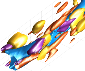
  $z$-directions and in time. The instantaneous flow field obtained in the streamwise-minimal (A3) case is presented in figure 1, in comparison with the reference-case results. As shown by the streamwise-cross sectional view in figure 1(a), the streamwise-minimal case reproduces the characteristic flow features observed in the reference case quite well, exhibiting both the near-wall structures (vortical motions observed near the walls around $y/h\approx \pm 0.1$) and the very-large-scale structures (the high- and low- $u$ regions filling up the entire channel gap). In the $xz$-plane views at the channel centre ( $y/h=0.5$) given in figure 1(b), it is shown that high- and low- $u$ streaks corresponding to the very-large-scale structures are present in the reference case, and similar streaks are found in case A3 as well. It is also shown that the streamwise domain extent in case A3 is considerably smaller than in the reference case. Because of this reduced domain length, the spanwise meandering motions of these streaks with some splitting and/or merging, which can be clearly observed in the reference-case results, are not captured in case A3.

Figure 1. Snapshots of instantaneous velocity fields obtained in the A3 and reference cases on (a) streamwise cross-sectional ( $zy$-) planes at arbitrary streamwise positions and (b) the channel centre plane ( $xz$-plane at $y/h=0.5$). The colours in all panels represent the fluctuating streamwise velocity $u / U_{w}$ for the range shown in panel (a), and the black arrows in panel (a) indicate the in-plane velocity vectors with the length scale where $1h$ length of the arrow corresponds to $U_{w}$.
Snapshots of instantaneous flow fields obtained in the spanwise-minimal case, case B2, are presented in figure 2. As shown by the middle plane slice ( $xz$-plane at $y/h=0.5$) given in panels (a) and (c), high- and low-speed streaks are observed with spanwise meanderings. However, as shown in panel (b), unlike in the streamwise-minimal and reference cases, there is no very-large-scale structure that fills up the entire channel gap in this case, which is clearly due to the narrow spanwise domain size. As the spanwise domain size is half the channel gap $h$, the structures that fit within this spanwise domain cannot be tall enough to penetrate the whole channel in the wall-normal direction.

Figure 2. Snapshots of instantaneous velocity fields obtained in case B2: (a) a wide view of the  $xz$-plane at the channel centre; (b) a streamwise cross-sectional view at $x=0.5L_x$ ( $=48.0h$); (c) a magnified view of the region in panel (a) marked by the red-dashed rectangle. The colours and the black vectors have the same meanings as in figure 1.
Figure 3 compares the mean streamwise velocity profiles obtained in the various computation runs in (a) the outer and (b) the inner scalings, and one can also find in table 1 the values of the friction Reynolds number  $Re_\tau =u_\tau (h /2)/\nu$, where $u_\tau$ is the friction velocity, defined as $u_\tau = \sqrt {\nu \mathrm {d}U/\mathrm {d} y|_{wall}}$. As one can see in figure 3, the mean velocity profiles obtained in the series of case A are all in quite good agreement with the reference case, while the results in the series of case B and case C indicate the influence of reducing $L_z$. The mean velocity profile deviates increasingly from the reference-case results as $L_z$ decreases, clearly corresponding to the disappearance of the very-large-scale structures in these cases as shown in figure 2. It is also seen in figure 3(b) that the logarithmic region of the mean velocity profile is hardly visible in these cases. Consistently with these mean velocity profiles, the $Re_\tau$ values obtained in cases A1–A3 agree well with the reference value (see table 1); even in the case of the minimal streamwise domain length (case A3) the deviation from the reference value is only 0.5 %. On the other hand, the values of $Re_\tau$ obtained in cases B1 and B2 clearly decrease as the spanwise domain length $L_z$ decreases.

Figure 3. Mean streamwise velocity profiles obtained with different computational domain sizes presented in (a) outer and (b) inner scalings. The colours of the lines represent the different series of computations: blue, the series of case A; red, case B; yellow, case C; black, the reference case. The grey dashed lines in panel (b) represent  $U^+=y^+$ and $U^+=1/\kappa \log y^+ +B$ with $\kappa =0.41$ and $B=5.1$. Note that the line for the reference case (black solid line) is hardly visible, as that for case A1 (blue solid line) is almost on top of it.
Figure 4 presents the profiles of the Reynolds stresses  $\langle u^2 \rangle$, $\langle v^2 \rangle$, $\langle w^2 \rangle$ and $-\langle uv \rangle$ scaled by the wall speed $U_{w}$. The Reynolds stresses are clearly affected by reducing $L_x$ as well as $L_z$, unlike the mean velocity profile. As shown in figure 4(a–c), reducing $L_z$ to the minimal size $L_z/h=0.5$ clearly suppresses the fluctuations of all velocity components, corresponding to the suppression of the very-large-scale structures in these cases. On the other hand, reducing $L_x$ increases the streamwise velocity fluctuation $\langle u^2 \rangle$ while decreasing the wall-normal and spanwise components $\langle v^2 \rangle$ and $\langle w^2 \rangle$. In particular, the wall-parallel components $\langle u^2 \rangle$ and $\langle w^2 \rangle$ are affected noticeably, while the influence on the wall-normal component $\langle v^2 \rangle$ is moderate. It also should be mentioned here that the sum of these fluctuations, $\langle u^2 \rangle + \langle v^2 \rangle + \langle w^2 \rangle$, is less affected by the change in $L_x$ (not shown), indicating that the energy redistribution between them is suppressed by reducing $L_x$. Such tendencies agree well with the DNS of turbulent channel flow with streamwise-minimal domains by Abe et al. (Reference Abe, Antonia and Toh2018). The profiles of the Reynolds shear stress $-\langle uv \rangle$ are also given in figure 4(d). As shown here the profile of $-\langle uv \rangle$ is insensitive to $L_x$, while reducing $L_z$ remarkably suppresses $-\langle uv \rangle$, which clearly corresponds, again, to the disappearance of the very-large-scale structures.

Figure 4. Profiles of the Reynolds stresses scaled by  $U_{w}^2$ obtained with different computational domain sizes: (a) $\langle u^2 \rangle$, (b) $\langle v^2 \rangle$, (c) $\langle w^2 \rangle$ and (d) $-\langle uv \rangle$. The colours and styles of the lines represent the same computation cases as in figure 3.
Figure 5 gives the budget of the transport equation of the turbulent kinetic energy  $k_t = (\langle u^2 \rangle +\langle v^2 \rangle +\langle w^2 \rangle )/2$ and the Reynolds shear stress $-\langle uv \rangle$ obtained in the streamwise- and spanwise-minimal cases. Here, the transport equation of the Reynolds stress $\langle u_i u_j \rangle$ is defined as
 \begin{equation} \left( \frac{\partial }{\partial t} + U_k \frac{\partial }{\partial x_k} \right) \langle u_i u_j \rangle = P_{ij} - \varepsilon_{ij} + \varPi_{ij} + D^\nu_{ij} + D^p_{ij} + D^t_{ij},\end{equation}
where the terms on the right-hand side are the production ( $P_{ij}$), viscous dissipation ( $\varepsilon _{ij}$), pressure–strain correlation ( $\varPi _{ij}$), viscous diffusion ( $D^\nu _{ij}$), pressure transport ( $D^p_{ij}$) and turbulent transport ( $D^t_{ij}$), which are defined, respectively, as
 \begin{gather} P_{ij} = - \langle u_i u_k \rangle \frac{\partial U_j}{\partial x_k} - \langle u_j u_k \rangle \frac{\partial U_i}{\partial x_k}, \quad \varepsilon_{ij} = 2 \nu \left \langle \frac{\partial u_i}{\partial x_k} \frac{\partial u_j}{\partial x_k} \right \rangle, \end{gather}
 \begin{gather}\varPi_{ij} = \frac{1}{\rho} \left \langle p \left( \frac{\partial u_i}{\partial x_j} + \frac{\partial u_j}{\partial x_i} \right) \right \rangle, \quad D^\nu_{ij} = \nu \frac{\partial ^2 \langle u_i u_j \rangle}{\partial x_k^2}, \end{gather}
 \begin{gather}D^p_{ij} = - \frac{1}{\rho} \frac{\partial }{\partial x_k} ( \langle p u_i \rangle \delta_{ik} + \langle pu_j \rangle \delta_{jk} ), \quad D^t_{ij} = -\frac{\partial \langle u_i u_j u_k \rangle}{\partial x_k}. \end{gather}
The profiles of these terms for the transport equation of  $k_t$ scaled by the wall units are presented in figure 5(a). Note that the pressure–strain correlation is not presented here as $\varPi _{uu}+\varPi _{vv}+\varPi _{ww}=0$. As shown, no significant difference between the streamwise-minimal and reference cases is observed for any term, whereas the budget given by the spanwise-minimal case gives production and viscous terms that are clearly larger in magnitude, particularly in the channel-central region. The budget of the Reynolds-shear-stress transport is also presented in figure 5(b). In the streamwise-minimal case, while the magnitude of the production $P_{-uv}$ and the pressure-related terms $\varPi _{-uv}+D^p_{-uv}$ are somewhat underestimated as compared to the reference-case results, the other terms are in quantitative agreement. In the budget given by the spanwise-minimal case, the production and the pressure-related terms are overestimated, similarly to the production and viscous terms in the turbulent kinetic energy budget, and it is also observed that the spatial transport term $D^t_{-uv}$ shows a certain discrepancy from the reference case.

Figure 5. Transport budget of the turbulent kinetic energy  $k_{t}=\langle u_i u_i \rangle +\langle v^2 \rangle +\langle w^2 \rangle )/2$ and the Reynolds shear stress $-\langle uv \rangle$ scaled by $u_\tau ^4 / \nu$: black solid lines, the reference case; blue chained lines, case A3; red dashed lines, case B2. The visc. terms and the press. terms respectively represent the sum of the viscous dissipation and diffusion terms and the sum of the pressure transport and pressure–strain correlation terms. The pressure transport term in (a) and viscous terms in (b) are presented with thinner lines for easier distinction. The upper abscissa of each panel represents the wall-normal height in wall units, $y^+=y u_\tau /\nu$, evaluated based on the results of the reference case.
Figure 6 presents the profiles of the pressure–strain correlations  $\varPi _{uu}$, $\varPi _{vv}$ and $\varPi _{ww}$, comparing the results of the reference and streamwise-minimal (A3) cases. As shown here, the magnitudes of all components of the pressure–strain correlations are smaller in case A3 than in the reference case. This indicates that the inter-component energy transfer from $\langle u^2 \rangle$ to the other components is suppressed in case A3, which is attributable to the observation in figure 4 that $\langle u^2 \rangle$ in this case is larger and the other components are smaller than in the reference case. The same tendency was also reported in earlier simulations of turbulent channel flow (Abe & Antonia Reference Abe and Antonia2016; Abe et al. Reference Abe, Antonia and Toh2018). Such suppression of the pressure–strain correlation in the streamwise-minimal case is addressed in detail based on the spectral analysis in § 3.2.

Figure 6. Profiles of the pressure–strain redistribution terms  $\varPi _{uu}$ (blue), $\varPi _{vv}$ (red) and $\varPi _{ww}$ (yellow), comparing the results obtained in the reference case (solid lines) and case A3 (dashed lines). The values are scaled by $u_\tau ^4/\nu$, and the upper abscissa represents the wall-normal height in wall units, $y^+=y u_\tau /\nu$, evaluated based on the results of the reference case.
The streamwise-minimal (A3) case also successfully reproduces the reference-case results in terms of the spectral energy distributions. Figure 7 presents the distributions of the premultiplied spanwise one-dimensional spectra of the streamwise turbulent energy  $k_z E^z_{uu}(y,k_x)$, comparing the results obtained in the reference and the streamwise-minimal cases. Here $k_z$ is the spanwise wavenumber $k_z=2{\rm \pi} /\lambda _z$, where $\lambda _z$ is the spanwise wavelength. As shown in the figure, the spectrum distributions obtained in these two cases are in fairly good agreement, in that both indicate two energy peaks: one located in the near-wall region at relatively small wavelengths $\lambda _z^+=\lambda _z u_\tau /\nu \approx 100$, and the other located at the channel centre at large wavelengths $\lambda _z/h \approx 2$. In particular, the energy peak at the larger wavelengths spreads broadly in the $y$-direction and reaches the near-wall region where the near-wall energy peak is located at smaller wavelengths. These spectral energy peaks clearly corresponds to the near-wall and the very-large-scale structures observed in figure 1(a). As described here, in turbulent plane Couette flow the energy peaks representing the inner and outer structures are observed clearly separated even at the relatively low Reynolds number $Re_\tau \approx 126$ investigated in the present study, which is due to the non-zero mean velocity gradient at the channel centre.

Figure 7. Space–wavelength ( $y$–
$y$– $\lambda _z$) diagrams of the spanwise one-dimensional spectra of the streamwise turbulent energy $E_{uu}^z$ in (a) the reference case and (b) case A3 (the streamwise-minimal case). The values are scaled by $u_\tau ^2$.
As described so far, the streamwise-minimal case reproduces the reference-case results fairly well despite the substantially limited degree of freedom in the streamwise direction, while the effect of reducing  $L_z$ is shown to be, as expected, remarkable mainly because the very-large-scale structure disappears with insufficient spanwise domain width. In the following section, the results provided by the streamwise- and spanwise-minimal domains are further examined based on the spectral analysis of the Reynolds stress transport. The focus is put, in the streamwise-minimal case, on why the streamwise-minimal domain still successfully reproduces the reference case results, while in the spanwise-minimal case the role of the interaction between the near-wall and very-large-scale structures in the Reynolds-stress transport is addressed.
3.2. Spectral analysis on the effect of reducing  $L_x$
$L_x$

In this section, we analyse the streamwise spectra of the Reynolds stresses and their transport in the streamwise-minimal case. Figure 8(a) compares the space–wavelength ( $y$–
$y$– $\lambda _x$) diagrams of the premultiplied streamwise one-dimensional spectra of the streamwise turbulent energy $k_x E^x_{uu}(y,k_x)$. As shown here, the $E^x_{uu}$ distribution obtained in the reference case shows both energy peaks corresponding to the near-wall structure (the one located at small wavelength $\lambda _x^+ \approx 600$) and the very-large-scale structure (the broad band of energy at large wavelength $\lambda _x/h \approx 48$), similarly to the spanwise energy spectrum $E^z_{uu}(y,k_z)$ in figure 7. It should be noted here that not only the broad band of energy at large $\lambda _x$ but also the near-wall peak is located in the wavelength range $\lambda _x^+>400$, and therefore in the streamwise-minimal case (A3) both of them are located outside the $y$–
$y$– $\lambda _x$ diagram of $k_x E^x_{uu}$ presented here. Instead, in the streamwise-minimal case, both the inner and outer peaks of the turbulent energy spectrum are accounted for by the $x$-independent mode, i.e. the Fourier mode at $k_x=0$ (or at $\lambda _x=\infty$). This is depicted in figure 8(b), where $E^x_{uu}(y,0) {\rm \Delta} k_x$ (here ${\rm \Delta} k_x = 2{\rm \pi} /L_x$), i.e. the amount of the streamwise turbulent energy on the Fourier mode at $k_x=0$, in the streamwise-minimal case is compared to the energy integrated over the range $\lambda _x/h > 1.6$,
 \begin{equation} \int^\infty_{\log 1.6h} k_x E^x_{uu}\, \mathrm{d} (\log\lambda_x) \left(= \int^{2{\rm \pi}/1.6h}_0 E^x_{uu}\, \mathrm{d}k_x \right),\end{equation}
in the reference case. As shown, the  $x$-independent Fourier mode in the streamwise-minimal case accounts for the equivalent fraction of the total $\langle u^2 \rangle$, up to 80 % of $\langle u^2 \rangle _{max}$, to the $\lambda _x/h>1.6$ range in the reference case. This means that the high- and low- $u$ streaks in both the near-wall and channel-core regions are $x$-independent in the streamwise-minimal case.

Figure 8. (a) Space–wavelength ( $y$–
$y$– $\lambda _x$) diagrams of premultiplied streamwise one-dimensional spectra of the streamwise turbulent energy $k_x E^x_{uu}$ obtained in (left) the reference case and (right) the streamwise-minimal (A3) case. The horizontal black dashed lines represent the streamwise domain size in the streamwise-minimal case, $\lambda _x/h=1.6$. (b) Profiles of streamwise turbulent energy spectra integrated for the wavelength range $\lambda _x/h > 1.6$ (i.e. $0 < k_xh < 2{\rm \pi} /1.6$) in (blue) the reference case and (red) the streamwise-minimal (A3) case. Note that, in case A3, $\int ^{2{\rm \pi} /1.6h}_0 E^x_{uu}(y,k_x)\, \mathrm {d} k_x = E^x_{uu}(y,0) {\rm \Delta} k_x$, where ${\rm \Delta} k_x = 2 {\rm \pi}/L_x$, since the $x$-independent mode is the only Fourier mode in the integrated $k_x$ range due to the limited domain size $L_x$. $\langle u^2 \rangle _{max}$ is the maximum value of the $\langle u^2 \rangle$ profile presented in figure 4(a).
The streamwise one-dimensional spectra of the cross-streamwise velocity fluctuations  $E^x_{vv}$ and $E^x_{ww}$ obtained in the reference and streamwise-minimal cases are also presented in figure 9. Note that the colour scale for the $k_x E^x_{vv}$ and $k_x E^x_{ww}$ distributions shown here is the same as in figure 8(a), showing that the magnitudes of $E^x_{vv}$ and $E^x_{ww}$ are relatively small compared to the streamwise turbulent energy $E^x_{uu}$. The results obtained in the reference case, given in figure 9(a), show that the spectral energies of $\langle v^2 \rangle$ and $\langle w^2 \rangle$ are mainly distributed in the relatively-small-wavelength range $\lambda _x/h<1.6$, and therefore, unlike the distribution of $E^x_{uu}$, their distributions are not significantly affected in the streamwise-minimal case, as shown in figure 9(b).

Figure 9. Space–wavelength ( $y$–
$y$– $\lambda _x$) diagrams of premultiplied streamwise one-dimensional spectra of the wall-normal turbulent energy $k_x E^x_{vv}$ and the spanwise turbulent energy $k_z E^x_{ww}$ obtained in (a) the reference case and (b) the streamwise-minimal (A3) case. The values are scaled by $u_\tau ^2$, and the colour scale is the same as in figure 8(a).
The transport equation of the Reynolds stress spectra can be derived by decomposing the Reynolds-stress transport equation (3.1) into the spectral contribution from each wavenumber, as done by, for example, Mizuno (Reference Mizuno2016), Lee & Moser (Reference Lee and Moser2015, Reference Lee and Moser2019) and Kawata & Alfredsson (Reference Kawata and Alfredsson2018, Reference Kawata and Alfredsson2019). The transport equation of the streamwise one-dimensional spectra of the Reynolds stress  $E^x_{ij}$ is written as
 \begin{equation} \left( \frac{\partial }{\partial t} + U_k \frac{\partial }{\partial x_k} \right) E^x_{ij} = pr^x_{ij} - \epsilon^x_{ij} + \pi^x_{ij} + d^{p,x}_{ij} + d^{\nu,x}_{ij} + d^{t,x}_{ij} + tr^x_{ij}, \end{equation}
where the first six terms on the right-hand side represent the spectral contribution from each streamwise wavenumber to the corresponding terms in the overall transport equation (3.1), whereas the last term  $tr^x_{ij}$ is an additional term that represents the interscale transfer of the Reynolds stress between different streamwise wavenumbers. Here the spectral Reynolds-stress transport equation (3.6) is derived by the same procedure as that of Kawata & Alfredsson (Reference Kawata and Alfredsson2019), which is briefly described in appendix A.
Figure 10(a) presents the  $y$–
$y$– $\lambda _x$ diagrams of the premultiplied spectral energy production $k_x pr^x_{uu}$, comparing the results in the reference and the streamwise-minimal cases. Similarly to the distribution of the streamwise energy spectrum $E^x_{uu}$, most of the spectral energy production $pr^x_{uu}$ is distributed in the relatively-large-wavelength range $\lambda _x^+>400$ in the reference case. In the streamwise-minimal case, on the other hand, the corresponding energy productions occur on the $x$-independent mode as shown by figure 10(b), where $pr^x_{uu}(y,0) {\rm \Delta} k_x$ in the streamwise-minimal case is shown to be comparable to the integrated production $\int ^{2{\rm \pi} /1.6h}_0 pr^x_{uu}\, \mathrm {d}k_x$ in the reference case. This indicates that the overall production $P_{uu}$ mainly represents the generation of $x$-independent streaks in the streamwise-minimal case.

Figure 10. Distributions of the streamwise one-dimensional spectra of the streamwise turbulent energy production  $pr^x_{uu}$ obtained in the reference case and the streamwise-minimal (A3) case, presented in the same manner as in figure 8: (a) $y$–
$y$– $\lambda _x$ diagrams of $k_x pr^x_{uu}$; (b) profiles of $pr^x_{uu}$ integrated for $\lambda _x/h > 1.6$ ( $0<k_xh<2{\rm \pi} /1.6$). Note that, in case A3, $\int ^{2{\rm \pi} /1.6h}_0 pr^x_{uu}(y,k_x)\, \mathrm {d} k_x=pr^x_{uu}(y,0) {\rm \Delta} k_x$. $P_{uu,max}$ represents the maximum value of the turbulent energy production $P_{uu}$.
Figure 11 presents the interscale transfer of the streamwise turbulent energy  $tr^x_{uu}$. As shown by the space–wavelength diagrams in panel (a), in the reference case the turbulent energy, which is produced by $pr^x_{uu}$ at large wavelengths as presented in figure 10(a), is transferred towards smaller wavelengths throughout the channel, and the streamwise-minimal-case result reproduces quite well the $tr^x_{uu}$ distribution of the reference case in the range $\lambda _x/h < 1.6$. It is particularly interesting to note here that the boundary between the energy-donating and -receiving $\lambda _x$ ranges in the reference case appears to be rather independent of $y$ and to coincide with the streamwise-minimal domain size $L_x=1.6h$, as indicated by the black dashed line. In the streamwise-minimal case, the energy gained in the $\lambda _x/h<1.6$ range is supplied entirely from the $x$-independent mode, since this is the only mode in the range $\lambda _x/h > 1.6$. Figure 11(b) compares the total amount of energy removed from the wavelength range $\lambda _x/h>1.6$, i.e. $\int ^{2{\rm \pi} /1.6h}_0 tr^x_{uu}\, \mathrm {d}k_x$, in the reference case to the energy transfer from the $x$-independent mode $tr^x_{uu}(y,0) {\rm \Delta} k_x$ in the streamwise-minimal case. As shown here, $tr^x_{uu}(y,0) {\rm \Delta} k_x$ in the streamwise-minimal case accounts for the equivalent energy transfer to $\int ^{2{\rm \pi} /1.6h}_0 tr^x_{uu}\, \mathrm {d}k_x$ in the reference case.

Figure 11. Distributions of the interscale transport of the streamwise turbulent energy in the streamwise wavenumber direction  $tr^x_{uu}$ obtained in the reference case and the streamwise-minimal (A3) case, presented in the same manner as in figure 8. Note that, in case A3, $\int ^{2{\rm \pi} /1.6h}_0 tr^x_{uu}(y,k_x)\, \mathrm {d} k_x=tr^x_{uu}(y,0) {\rm \Delta} k_x$.
The good agreement between the  $tr^x_{uu}$ distributions obtained in the reference and streamwise-minimal cases, as shown in figure 11, may give us an insight into the mechanism of the interscale energy transfer. From the view point of the Fourier mode analysis, the interscale energy transfer is generally caused by triad interactions between three wavenumbers. In the streamwise-minimal case, the $x$-independent mode is the only mode in the range $\lambda _x/h>1.6$, and therefore the energy transfer from the $x$-independent mode to smaller scales across $\lambda _x/h=1.6$ is caused by interaction between $k_x=0$ and non-zero wavenumbers $k_x=\pm 2{\rm \pi} m/1.6h$ (where $m$ is a positive integer). The agreement between the $tr^x_{uu}$ distributions given in figure 11(b) indicates that the energy transfer from larger to smaller scales across $\lambda _x/h=1.6$ in the reference case is also mainly caused by similar direct interactions between widely-separated wavenumbers, i.e. by the triad interactions between very small $k_x$ ( $\approx 0$) and large ( $k_x=\pm 2 {\rm \pi}m/L_x$) wavenumbers; if other triad combinations of moderate wavenumbers played important roles, the agreement shown in figure 11(b) between the streamwise-minimal case and the reference case would not have been achieved, because such triad interactions cannot be simulated in the streamwise-minimal case.
Figure 12 presents the distribution of the pressure–strain cospectrum  $\pi ^x_{uu}$ comparing the results obtained in the reference and the streamwise-minimal cases. One can see here that the pressure–strain cospectrum is mostly significant in the relatively-small-wavelength range $\lambda _x/h < 1.6$ throughout the channel, and the $\pi ^x_{uu}$ distribution obtained in the streamwise-minimal case reproduces the results of the reference case fairly well. This tendency of $\pi ^x_{uu}$ is consistent with the distributions of $E^x_{vv}$ and $E^x_{ww}$ shown in figure 9. It also should be noted here that the $\pi ^x_{uu}$ distribution of the reference case shows a certain contribution from the range $\lambda _x/h >1.6$, which cannot be taken into account in the streamwise-minimal case because $\pi ^x_{uu}=0$ at $k_x=0$, as $\partial u/\partial x = 0$ for any $x$-independent structure. The contributions from the relatively-small- $\lambda _x$ range $\lambda _x/h<1.6$ are evaluated as $\int ^{\infty }_{2{\rm \pi} /1.6h} \pi ^x_{uu}\, \mathrm {d} k_x$ for both the reference and streamwise-minimal cases and are compared in figure 12(b). Note here that for the streamwise-minimal case $\int ^{\infty }_{2{\rm \pi} /1.6h} \pi ^x_{uu}\, \mathrm {d} k_x=\int ^{\infty }_{0} \pi ^x_{uu}\, \mathrm {d} k_x=\varPi _{uu}$, since the contribution from the range $\lambda _x/h>1.6$ ( $0<k_xh<1/1.6$) is zero as explained above. As shown, the profile of $\int ^{\infty }_{2{\rm \pi} /1.6h} \pi ^x_{uu}\, \mathrm {d} k_x$ given by the reference case is, of course, somewhat smaller in magnitude than the overall pressure–strain correlation $\varPi _{uu}$ of the reference case, and the $\varPi _{uu}$ obtained in the streamwise-minimal case has equivalent magnitude to $\int ^{\infty }_{2{\rm \pi} /1.6h} \pi ^x_{uu}\, \mathrm {d} k_x$ in the reference case. This indicates that the suppression of $\varPi _{uu}$ in the streamwise-minimal case, observed in figure 6, occurs mainly because the energy-containing streaks are forced to be $x$-independent because of the limited streamwise domain size, and therefore do not induce the energy redistribution from $\langle u^2 \rangle$ to the other components on their own.

Figure 12. Distributions of the streamwise one-dimensional cospectra of the pressure–strain correlation  $\pi ^x_{uu}$ obtained in the reference case and the streamwise-minimal (A3) case, presented in a similar manner to figure 8. Note that, in case A3, $\int ^\infty _{2{\rm \pi} /1.6h} \pi ^x_{uu} (y,k_x)\, \mathrm {d}k_x = \varPi _{uu}(y)$. The overall pressure–strain correlation $\varPi _{uu}$ in the reference case (black) is also compared in panel (b).
The spectral analysis on the turbulent energy transport described above has shown that, in the reference case, the streamwise turbulent energy  $\langle u^2 \rangle$ is produced mainly at relatively large streamwise wavelengths $\lambda _x^+>400$, and is then transferred by the interscale transport $tr^x_{uu}$ towards the smaller-wavelength range, where the energy is redistributed to the cross-streamwise components by the pressure–strain correlation. In the streamwise-minimal case, the energy production mainly occurs at $k_x=0$ in both the near-wall and core regions of the channel, indicating that both streaks of the near-wall and very-large-scale structures are forced to be $x$-independent, and the energy is transferred from the $x$-independent mode to all other modes in the range $\lambda _x^+<400$. Importantly, in spite of this effect of the limited degree of freedom, the streamwise-minimal domain still reproduces the flow field obtained in the reference case fairly well, as shown in § 3.1. This indicates that the interactions between the $x$-independent streaks and relatively small structures in the range $\lambda _x^+<400$ are the essential dynamics for both the inner and outer structures, and the spanwise meanderings of the streaks observed in the reference case (such as those presented in figure 1b) are, therefore, rather unimportant features of wall turbulence, as previously suggested by Abe et al. (Reference Abe, Antonia and Toh2018). Furthermore, as discussed above, the good agreement between the $tr^x_{uu}$ distributions shown in figure 11(b) indicates that $tr^x_{uu}$ mainly represents direct energy transfers between widely-separated scales, i.e. between very large ( $\lambda _x \gg h$) and relatively small ( $\lambda _x^+<400$) wavelengths, via instabilities, for instance, rather than successive energy transfers from one scale to a neighbouring slightly-smaller scale via a turbulent energy cascade.
3.3. Spectral analysis on the effect of reducing $L_z$

Next, we investigate the Reynolds stress transports in the spanwise-minimal (B2) case, emphasising the difference between the interscale transfer effects in the reference and spanwise-minimal cases, in order to elucidate the role of the interaction between the inner and outer structures. In this investigation we focus on the spanwise spectra of the Reynolds stresses  $E^z_{ij}(y,k_z)$. Their transport equation is written as
 \begin{equation} \left( \frac{\partial }{\partial t} + U_k \frac{\partial }{\partial x_k} \right) E^z_{ij} = pr^z_{ij} - \epsilon^z_{ij} + \pi^z_{ij} + d^{p,z}_{ij} + d^{\nu,z}_{ij} + d^{t,z}_{ij} + tr^z_{ij}, \end{equation}
similarly to (3.6). The first six terms on the right-hand side now represent the spectral contribution from each spanwise wavenumber to the corresponding term in (3.1), and the last term  $tr^z_{ij}$ indicates the interscale transfer in the spanwise wavenumber direction.
Figure 13(a) presents the  $y$–
$y$– $\lambda _z$ diagrams of the interscale transport of the streamwise turbulent energy $tr^z_{uu}$. As one can see here, the $tr^z_{uu}$ distribution obtained in the reference case indicates that $\langle u^2 \rangle$ is transferred mainly from larger ( $\lambda _z/h\approx 2$) to smaller $\lambda _z$, while in the near-wall region transport from smaller to larger $\lambda _z$ is also found. This is in contrast to the interscale transfer in the streamwise wavenumber direction $tr^x_{uu}$, which shows only transport from larger to smaller wavelengths $\lambda _x$ throughout the channel, as presented in figure 11(a). This point is further addressed in § 4.4. In the spanwise-minimal case (case B2), the $tr^z_{uu}$ distribution reproduces the reference-case results fairly well for the wavelength range $\lambda _z/h<0.5$. The energy is mainly removed from $\lambda _z/h=0.5$ and partly transferred to smaller $\lambda _z$ in the near-wall region; the rest is transferred to the $z$-independent mode, as indicated by the large positive values of $tr^z_{uu}(y,0) {\rm \Delta} k_z$ in the spanwise-minimal case, presented in figure 13(b). The $tr^z_{uu}(y,0) {\rm \Delta} k_z$ profile is compared with the amount of energy transferred from the range $\lambda _z/h<0.5$ to $\lambda _z/h>0.5$ in the reference case, and one can see that the reversed energy transfer to the $z$-independent mode in the spanwise-minimal case captures qualitatively the tendency of the corresponding interscale energy transfer in the reference case, particularly the inverse interscale transfer in the near-wall region. Such agreement between the reference and spanwise-minimal cases is somewhat surprising, given that the instantaneous flow field obtained in the spanwise-minimal case is qualitatively different from that of the reference case, in that the very-large-scale structure does not exist in the channel-core region, as observed in § 3.1.

Figure 13. (a) Space–wavelength ( $y$–
$y$– $\lambda _z$) diagrams of the premultiplied interscale transport of the streamwise turbulent energy in the spanwise wavenumber direction $k_z tr^z_{uu}$ obtained in (left) the reference case and (right) the spanwise-minimal (B2) case. The horizontal black dashed lines represent the spanwise domain size in the spanwise-minimal case $\lambda _z/h=0.5$. (b) Profiles of the interscale transport $tr^z_{uu}$ integrated for the wavelength range $\lambda _z/h > 0.5$ (i.e. $0 < k_zh < 2{\rm \pi} /0.5$), in (blue) the reference case and (red) the spanwise-minimal (B2) case. Note that, in case B2, $\int ^{2{\rm \pi} /0.5h}_0 tr^z_{uu}(y,k_z)\, \mathrm {d} k_z=tr^z_{uu}(y,0) {\rm \Delta} k_z$, where ${\rm \Delta} k_z=2 {\rm \pi}/L_z$, due to the limited domain size $L_z$.
Kawata & Alfredsson (Reference Kawata and Alfredsson2018) experimentally investigated the spectral transport of the Reynolds stresses in a turbulent plane Couette flow based on spanwise Fourier mode analysis and showed that the Reynolds shear stress  $-\langle uv \rangle$ is transferred from smaller to larger $\lambda _z$ throughout the channel. This inverse interscale transport of the Reynold shear stress is also observed in the present study. As shown in figure 14(a), the distribution of the interscale Reynolds-shear-stress transport $tr^z_{-uv}$ obtained in the reference case shows transfer from smaller to larger $\lambda _z$ throughout the channel, consistently with the experimental observations of Kawata & Alfredsson (Reference Kawata and Alfredsson2018). The results in the spanwise-minimal case also reproduce the same tendency, with the Reynold shear stress mainly transferred from $\lambda _z/h \approx 0.25$ to larger wavelengths. As indicated by the comparison between $\int ^{2{\rm \pi} /0.5h}_0 tr^z_{-uv}\, \mathrm {d}k_z$ in the reference case and $tr^z_{-uv}(y,0) {\rm \Delta} k_z$ in the spanwise-minimal case, the interscale transfer between the $\lambda _z/h <0.5$ range and the $z$-independent mode in the spanwise-minimal case is a good qualitative representation of the inverse interscale transfers of the Reynolds shear stress in the reference case.

Figure 14. Distributions of the interscale transport of the Reynolds shear stress in the spanwise wavenumber direction  $tr^z_{-uv}$ obtained in the reference case and the spanwise-minimal (B2) case, presented in the same manner as in figure 13.
As described above, the spanwise-minimal case gives the same tendencies of the interscale transport  $tr^z_{ij}$ as observed in the reference case, including the inverse interscale transport of the Reynolds shear stress, despite the fact that the very-large-scale structures do not exist in this case. This suggests that the interscale transfers observed through spanwise Fourier mode analysis may not represent the effect of the interaction between the near-wall and very-large-scale structures. This is further discussed in § 4.4.
4. Discussions
4.1. On the relation between the spectral Reynolds-stress transport and the self-sustaining process of coherent structures
In § 3.2, we have shown that the streamwise length scales split mainly into two wavelength ranges: the larger- $\lambda _x$ range $\lambda _x^+>400$, in which the energy is produced by $pr^x_{uu}$ and taken by the interscale energy transfer $tr^x_{uu}$, and the smaller- $\lambda _x$ range $\lambda _x^+<400$, where the energy is supplied from larger $\lambda _x$ by $tr^x_{uu}$ and redistributed by the pressure–strain correlation $\pi ^x_{uu}$. The boundary between these two $\lambda _x$ ranges has been found to be nearly constant throughout the channel and to coincide with the streamwise-minimal domain length $L_x^+ \approx 400$. In the streamwise-minimal case, the streamwise wavelengths in the energy-producing (and -donating) $\lambda _x$ range are accounted for only by the streamwise-independent (i.e. $k_x=0$) mode, due to the limited degree of freedom, but otherwise the spectral energy transports observed in the reference case are basically retained, and thus the streamwise-minimal case reproduces the reference-case results fairly well. Given that both the inner and outer structures are retained in the streamwise-minimal case, as shown in figures 1 and 7, these observations indicate that the energy production at very large streamwise wavelengths ( $k_x\approx 0$), the interscale energy transfer, and the energy redistribution at small wavelengths ( $\lambda _x^+<400$) are the essential energy transport processes for both the inner and outer structures.
In addition to the spectral energy transports described above, it should be further noted that the turbulent energy redistributed from  $\langle u^2 \rangle$ to $\langle v^2 \rangle$ results in the production of the Reynolds shear stress $P_{-uv}=\langle v^2 \rangle \, \mathrm {d}U/\mathrm {d} y$, which further leads to the reproduction of the streamwise turbulent energy $\langle u^2 \rangle$ as $P_{uu}=-2\langle uv \rangle \, \mathrm {d}U/\mathrm {d} y$. This closed-loop transport of the Reynolds stresses, consisting of production, interscale transfer and inter-component redistribution, resembles the scenario of the self-sustaining cycle of wall turbulence (Hamilton et al. Reference Hamilton, Kim and Waleffe1995; Waleffe Reference Waleffe1997): the significant $\langle u^2 \rangle$ production on the nearly- $x$-independent modes is very compatible with the generation of the $x$-independent $u$-streaks; the interscale energy transfer by $tr^x_{uu}$ is compatible with the streak instabilities; and the energy redistribution from $\langle u^2 \rangle$ to $\langle v^2 \rangle$ and $\langle w^2 \rangle$ at relatively small $\lambda _x$ is compatible with the generation of vortical structures from the streaks through their breakdown. While the self-sustaining process was originally proposed as the generating mechanism of the near-wall structures, recent studies (e.g. Hwang & Cossu Reference Hwang and Cossu2010, Reference Hwang and Cossu2011; Rawat et al. Reference Rawat, Cossu, Hwang and Rincon2015; Hwang & Bengana Reference Hwang and Bengana2016; Cossu & Hwang Reference Cossu and Hwang2017; de Giovanetti, Sung & Hwang Reference de Giovanetti, Sung and Hwang2017) have provided overwhelming evidence indicating that the large-scale structures in the logarithmic and outer layers are also essentially maintained by similar self-sustaining cycles, rather than by the influence of the smaller-scale structures near the wall. We now conjecture that the spectral energy transports observed in § 3.2 are closely related to each subprocess of the self-sustaining cycles of the inner and outer structures, and we examine this conjecture in detail in the following.
An insight supporting the correspondence between the streak instabilities and the interscale energy transport  $tr^x_{uu}$ is obtained by decomposing $tr^x_{uu}$. The interscale transport $tr^x_{ij}$ in (3.6) is obtained as
 \begin{equation} tr^x_{ij}(y,k_x) = - \frac{\partial Tr^x_{ij} (y,k_x)}{\partial k_x}, \end{equation}
where  $Tr^x_{ij}$, which represents the flux of the Reynolds stress in the streamwise wavenumber direction across $k_x$ from the larger- to the smaller-scale side, is defined as
 \begin{equation} Tr^x_{ij} = -\left \langle u^S_i u^S_k \frac{\partial u^L_j}{\partial x_k} \right \rangle -\left \langle u^S_j u^S_k \frac{\partial u^L_i}{\partial x_k} \right \rangle +\left \langle u^L_i u^L_k \frac{\partial u^S_j}{\partial x_k} \right \rangle +\left \langle u^L_j u^L_k \frac{\partial u^S_i}{\partial x_k} \right \rangle. \end{equation}
Here,  $u^L_i$ and $u^S_i$ are respectively the large- and small-scale parts of the fluctuating velocity $u_i$, obtained by applying low- and high-pass spatial filterings based on the streamwise Fourier mode with the cutoff wavenumber $k_x$ (see appendix A for details). Then the interscale flux of the streamwise turbulent energy $Tr^x_{uu}$ is expressed as
 \begin{align} Tr^x_{uu} &= \underbrace{-2 \left \langle u^S u^S \frac{\partial u^L}{\partial x} \right \rangle}_{Tr^{x,1}_{uu}} - \underbrace{2 \left \langle u^S v^S \frac{\partial u^L}{\partial y} \right \rangle}_{Tr^{x,2}_{uu}} \underbrace{-2 \left \langle u^S w^S \frac{\partial u^L}{\partial z} \right \rangle}_{Tr^{x,3}_{uu}} \nonumber\\ &\quad \underbrace{+2 \left \langle u^L u^L \frac{\partial u^S}{\partial x} \right \rangle}_{Tr^{x,4}_{uu}} + \underbrace{2 \left \langle u^L v^L \frac{\partial u^S}{\partial y} \right \rangle}_{Tr^{x,5}_{uu}} + \underbrace{2 \left \langle u^L w^L \frac{\partial u^S}{\partial z} \right \rangle }_{Tr^{x,6}_{uu}}, \end{align}
and therefore the interscale transport  $tr^x_{uu}$ is also decomposed as
 \begin{equation} tr^x_{uu} = tr^{x,1}_{uu} + tr^{x,2}_{uu} + tr^{x,3}_{uu} + tr^{x,4}_{uu} + tr^{x,5}_{uu} + tr^{x,6}_{uu}, \end{equation}
in accordance with  $Tr^x_{uu}$.
Figure 15(a) compares the contributions of two major terms on the right-hand side of (4.4) to the energy transfer on the  $x$-independent mode $tr^x_{uu}(y,0)$ in the streamwise-minimal case. Note that only $tr^{x,2}_{uu}(y,0)$ and $tr^{x,3}_{uu}(y,0)$ are presented here because the other terms are all zero, as explained in detail in appendix B. As shown here, the energy is transferred from the $x$-independent mode mostly due to $tr^{x,3}_{uu}$, which represents the effect of the spanwise velocity gradient by the larger structure $\partial u^L/\partial z$, as one can see from (4.3). This corresponds to the spanwise variation of $u$ induced by the $x$-independent structures. In the reference case, on the other hand, the energy is taken from finite wavelengths, unlike in the streamwise-minimal case, and therefore all the terms in the right-hand side of (4.4) can contribute to the interscale energy transfer from the large- $\lambda _x$ range. The contributions of all terms in the reference case are presented in figures 15(b) and 15(c) for a near-wall location $y^+=16$ and the channel centre, respectively. As shown in figure 15(b), the contribution by the third term $tr^{x,3}_{uu}$ is dominant at the near-wall location in the reference case at relatively large wavelengths ( $\lambda _x^+>400$). In particular, the energy transfer from very large wavelengths $\lambda _x^+>1000$ is entirely due to $tr^{x,3}_{uu}$, which is consistent with the observations in the streamwise-minimal case in figure 15(a). The other terms have roughly the same magnitude, and all become comparable to $tr^{x,3}_{uu}$ at relatively small wavelengths $\lambda _x^+ \approx 100$. The energy transferred by $tr^{x,3}_{uu}$ from large- to moderate- $\lambda _x$ ranges is further transferred towards the smaller- $\lambda _x$ range by the other terms, which may represent the turbulent energy cascade. The third term $tr^{x,3}_{uu}$ also plays a primary role in the interscale energy transport at the channel centre, as shown in figure 15(c). While the second term $tr^{x,2}_{uu}$ also shows a significant contribution, the contribution by $tr^{x,3}_{uu}$ is dominant at very large wavelengths $\lambda _x/h > 10$. The dominant contributions by $tr^{x,3}_{uu}$ at large $\lambda _x$ are consistent with the observations in earlier studies that the main mechanism of the streak instabilities is inflectional instability due to the spanwise variation of $u$ induced by the streaks (e.g. Swearingen & Blackbelder Reference Swearingen and Blackbelder1987; Hamilton et al. Reference Hamilton, Kim and Waleffe1995; Jiménez & Pinelli Reference Jiménez and Pinelli1999); thus, this supports our claim that $tr^x_{uu}$ in the relatively-large- $\lambda _x$ range is closely related to the streak instabilities in the self-sustaining process in both the near-wall and the central regions of the channel.

Figure 15. Comparison of various terms on the right-hand side of (4.3): (a) in the streamwise-minimal (A3) case, on the  $x$-independent mode across the channel; (b,c) in the reference case, (b) at the near-wall location $y^+=16$ ( $y/h=0.063$) and (c) at the channel centre $y/h=0.5$ across the whole $\lambda _x$ range investigated.
In order to more directly examine the correspondence between the Reynolds stress budgets and the self-sustaining process, we investigate the instantaneous flow fields obtained in case C, where both  $L_x$ and $L_z$ are as small as their minimal sizes; this is similar to the flow configuration employed by Hamilton et al. (Reference Hamilton, Kim and Waleffe1995) to observe the self-sustaining cycle. The instantaneous velocity field is decomposed into the $x$-independent mode $u_i^\prime =\langle u_i \rangle _x$ and the $x$-dependent mode $u_i^{\prime \prime }=u_i-u_i^\prime$ (here $\langle \rangle _x$ represents spatial averaging in the $x$-direction). Now we define the integrated turbulent energy on the $x$-independent mode as
 \begin{equation} \mathcal{E}^\prime_{uu} = \int^{0.195h}_{0} \langle {u^\prime}^2 \rangle_{xz}\, \mathrm{d} y, \end{equation}
and similarly we define the streamwise and lateral energies on the  $x$-dependent modes as
 \begin{equation} \mathcal{E}^{\prime \prime}_{uu} = \int^{0.195h}_{0} \langle {u^{\prime \prime}}^2 \rangle_{xz}\, \mathrm{d} y, \quad \mathcal{E}^{\prime \prime}_{vw} = \int^{0.195h}_{0} ( \langle {v^{\prime \prime}}^2 \rangle_{xz}+\langle {w^{\prime \prime}}^2 \rangle_{xz} )\, \mathrm{d} y; \end{equation}
their time series are presented in figure 16(a). Here  $\langle \rangle _{xz}$ indicates spatial averaging in the $x$- and $z$-directions. The integration range $0 \leq y/h \leq 0.195$ (or $0 \leq y^+ \leq 40$ in the viscous unit) is chosen based on the $\langle u^2 \rangle$ profile obtained in case C, so that most of the turbulent energy related to the coherent structures near the bottom wall is included (see figure 4). The time series of the integrated turbulent energies given in figure 16(a) present a typical periodic behaviour. It appears that they are well correlated with each other, and the fluctuations of the $x$-dependent energies $\mathcal {E}^{\prime \prime }_{uu}$ and $\mathcal {E}^{\prime \prime }_{vw}$ follow that of the $x$-independent streamwise energy $\mathcal {E}^{\prime }_{uu}$ with a slight delay. The time delays are quantified in figure 16(b), which presents the cross-correlation functions between $\mathcal {E}^{\prime }_{uu}$ and $\mathcal {E}^{\prime \prime }_{uu}$, and between $\mathcal {E}^{\prime }_{uu}$ and $\mathcal {E}^{\prime \prime }_{vw}$, defined as
 \begin{equation} C_{\mathcal{E}^{\prime}_{uu}}^{\mathcal{E}^{\prime \prime}_{uu}} (\tau) = \frac{\langle \mathcal{E}^{\prime}_{uu}(t) \mathcal{E}^{\prime \prime}_{uu} (t + \tau) \rangle}{\sqrt{\langle {\mathcal{E}^{\prime}_{uu}}^2 \rangle} \sqrt{\langle {\mathcal{E}^{\prime \prime}_{uu}}^2 \rangle}}, \quad C_{\mathcal{E}^{\prime}_{uu}}^{\mathcal{E}^{\prime \prime}_{vw}} (\tau) = \frac{\langle \mathcal{E}^{\prime}_{uu}(t) \mathcal{E}^{\prime \prime}_{vw} (t + \tau) \rangle}{\sqrt{\langle {\mathcal{E}^{\prime}_{uu}}^2 \rangle} \sqrt{\langle {\mathcal{E}^{\prime \prime}_{vw}}^2 \rangle}}.\end{equation}
As can be seen here, the correlation peaks of both cross-correlation functions are located at negative  $\tau$, around $\tau ^+\approx -50$, and $C_{\mathcal {E}^{\prime }_{uu}}^{\mathcal {E}^{\prime \prime }_{vw}}$ gives larger delay than $C_{\mathcal {E}^{\prime }_{uu}}^{\mathcal {E}^{\prime \prime }_{uu}}$. This indicates that the fluctuation of the $x$-independent streamwise turbulent energy $\mathcal {E}^\prime _{uu}$ is followed by that of the $x$-dependent energy $\mathcal {E}^{\prime \prime }_{uu}$, which is further followed by that of the lateral turbulent energy $\mathcal {E}^{\prime \prime }_{vw}$. This observed sequence of $\mathcal {E}^\prime _{uu}$, $\mathcal {E}^{\prime \prime }_{uu}$ and $\mathcal {E}^{\prime \prime }_{vw}$ indicates that they mainly represent the energies of $x$-independent streaks, wavy streaks and vortical structures of the self-sustaining process, respectively.

Figure 16. Time series and cross-correlation functions of integrated turbulent energies and Reynolds stress budgets obtained in case C: (a) time series of  $\mathcal {E}^\prime _{uu}$ (blue), $\mathcal {E}^{\prime \prime }_{uu}$ (red) and $\mathcal {E}^{\prime \prime }_{vw}$ (yellow) scaled by $u_\tau \nu$; (b) cross-correlation functions $C_{\mathcal {E}^\prime _{uu}}^{\mathcal {E}^{\prime \prime }_{uu}}$ (blue) and $C_{\mathcal {E}^\prime _{uu}}^{\mathcal {E}^{\prime \prime }_{vw}}$ (red); (c) time series of $\mathcal {P}^\prime _{uu}$ (blue), $\mathcal {T}_{uu}$ (red) and $\mathcal {R}_{uu}$ (yellow) scaled by $u_\tau ^3$; (d) cross-correlation functions $C_{\mathcal {E}^\prime _{uu}}^{\mathcal {P}^\prime _{uu}}$ (blue), $C_{\mathcal {E}^{\prime \prime }_{uu}}^{\mathcal {T}_{uu}}$ (red) and $C_{\mathcal {E}^{\prime \prime }_{vw}}^{\mathcal {R}_{uu}}$ (yellow). The vertical black dashed lines in panels (a) and (c) indicate the time range of the flow visualisation presented in figure 17.
Similarly, the integrated turbulent energy production on the  $x$-independent mode $\mathcal {P}^\prime _{uu}$, the integrated interscale energy flux from the $x$-independent towards the $x$-dependent modes $\mathcal {T}_{uu}$, and the integrated pressure–strain energy redistribution $\mathcal {R}_{uu}$ are defined as
 \begin{gather} \mathcal{P}^\prime_{uu} = \int^{0.195h}_0 \langle \widetilde{pr^x_{uu}} | _{k_x=0} {\rm \Delta} k_x \rangle_{xz}\, \mathrm{d} y = \int^{0.195h}_0 - 2 \langle u^\prime v^\prime \rangle_{xz} \frac{\mathrm{d}U}{\mathrm{d} y}\, \mathrm{d} y, \end{gather}
 \begin{gather}\mathcal{T}_{uu} = \int^{0.195h}_0 \langle \widetilde{Tr^{x,3}_{uu}} |_{k_x=0} \rangle_{xz}\, \mathrm{d} y = \int^{0.195h}_0 -2 \left \langle u^{\prime \prime} w^{\prime \prime} \frac{\partial u^\prime}{\partial z} \right \rangle_{xz}\, \mathrm{d} y, \end{gather}
 \begin{gather}\mathcal{R}_{uu} = \int^{0.195h}_0 \langle \widetilde{\varPi_{uu}} \rangle_{xz} (y)\, \mathrm{d} y =\int^{0.195h}_0 2 \left \langle p^{\prime \prime} \frac{\partial u^{\prime \prime}}{\partial x} \right \rangle_{xz}\, \mathrm{d} y, \end{gather}
where the tilde  $\widetilde {\:}$ indicates the instantaneous values of the spectral budget term that are not averaged in the $x$- or $z$-direction or in time. The times series of these integrated budget terms are presented in figure 16(c). These time series also indicate certain periodic behaviours and are significantly correlated with each other, similarly to those of the integrated turbulent energies in panel (a). Figure 16(d) presents cross-correlation functions $C_{\mathcal {P}^{\prime }_{uu}}^{\mathcal {E}^{\prime }_{uu}}$, $C_{\mathcal {T}_{uu}}^{\mathcal {E}^{\prime \prime }_{uu}}$ and $C_{\mathcal {R}_{uu}}^{\mathcal {E}^{\prime \prime }_{vw}}$, defined in the same manner as those in (4.7a,b). As shown here, all three cross-correlation functions have the maximum magnitude of correlation located at negative $\tau$ of the order of $\tau ^+ \approx 10$. This indicates that $\mathcal {E}^\prime _{uu}$, $\mathcal {E}^{\prime \prime }_{uu}$ and $\mathcal {E}^{\prime \prime }_{vw}$ respond immediately to the increase or decrease of the energy production $\mathcal {P}^\prime _{uu}$, the interscale energy transfer $\mathcal {T}_{uu}$ and the pressure–strain energy redistribution $\mathcal {R}_{uu}$, respectively. In particular, the peak magnitudes of these cross-correlation functions are all significantly high (more than 0.5), which also indicates the close causal relationship between these turbulent energies and the Reynolds stress budget terms.
Figure 17 presents flow visualisations of the instantaneous flow field at six different instants during the period indicated by black dashed lines in figure 16(a,c). In each panel, the region near the bottom wall,  $0 \leq y^+ \leq 60$, is visualised, and the coloured surfaces represent iso-surfaces of $u^+=-5$ (blue), $Q^+=-0.04$ (red), $\tilde {\varPi }_{uu}^+=-0.75$ (yellow) and $\widetilde {Tr_{uu}^{x,3}}^+ |_{k_x=0}=1.45$ (purple), where $Q$ is the second invariant of the velocity-gradient tensor. The instantaneous flow fields shown here are low-pass-filtered with a cutoff wavelength $k_{x,c}h/2{\rm \pi} =1.88$ ( $\lambda _{x,c}^+=118$) to allow clear visualisation of coherent structures, but most of the turbulent energies (more than 90 % of $\langle u^2 \rangle$ and 68 % of $\langle v^2 \rangle + \langle w^2 \rangle$) are still retained in the flow field visualised here. In panels (a–c) (from $t^+=1293$ to $t^+=1370$), the evolution of a low-speed streak is observed, and streamwise-elongated vortices are also found aligned with the streak. In particular, in panel (c) the streak has grown enough to penetrate the computational domain in the $x$-direction. This instant ( $t^+=1370$) actually corresponds to the peak of the $x$-independent streamwise turbulent energy $\mathcal {E}^\prime _{uu}$ in figure 16(a), and the $x$-dependent streamwise turbulent energy $\mathcal {E}^{\prime \prime }_{uu}$ is also increasing at this instant. Therefore the streak visualised in figure 17(c) is somewhat wavy. It can also be observed that the regions of significant interscale energy transfer from $x$-independent to $x$-dependent modes (purple) and inter-component energy transfer by pressure–strain correlation (yellow) start to appear around the streak. Panel (d) (at $t^+=1386$) corresponds to the peak of the interscale energy transfer $\mathcal {T}_{uu}$ in figure 16(c), and at this instant the $x$-dependent energy $\mathcal {E}^{\prime \prime }_{uu}$ in figure 16(a) is also saturated. Hence, the low-speed streak visualised in figure 17(d) is strongly wavy and surrounded by regions of significant interscale energy transfer. It is also observed that the pressure–strain energy redistribution is significant, and streamwise-elongated vortices visualised by $Q$ are evolving around the wavy streak. In panel (e) (at $t^+=1400$), the streak is shown to have already broken down. However, the regions of significant pressure–strain energy redistribution are still found, and vortical structures also remain. As time proceeds such vortical structures further evolve; as shown in panel (f), they remain after the low-speed streaks have become hardly visible, eventually giving rise to next streaks.

Figure 17. Visualisations of instantaneous flow fields in the region near the bottom wall ( $0 \leq y^+ \leq 60$) observed in case C at (a) $t^+=1253$, (b) $t^+=1293$, (c) $t^+=1370$, (d) $t^+=1386$, (e) $t^+=1400$ and (f) $t^+=1489$. The full range of the computational domain is shown in the $x$- and $z$-directions. The three-dimensional surfaces of different colours in each panel represent iso-surfaces of $u^+=-5$ (blue), $Q^+=-0.04$ (red), $\tilde {\varPi }_{uu}^+=-0.75$ (yellow) and $\widetilde {Tr_{uu}^{x,3}}^+ |_{k_x=0} =1.45$ (purple). The flow fields shown are low-pass-filtered at the cutoff wavenumber $k_{x,c}h/2{\rm \pi} =1.88$ ( $\lambda _{x,c}^+=118$) for clear visualisation of coherent structures.
The above observations in case C of the growth/breakdown of a streak and vortices in relation to the turbulent energy budget terms agree fairly well with the scenario of the self-sustaining cycle, and thus support our conjecture about their close relationship. Details of the balance between the spectral budget terms in case C are presented in figure 18(a) for a near-wall location  $y^+ = 16$. As shown here, the peak of the energy production, accounting for nearly 70 % of the overall energy production, is located at $k_x=0$. The interscale energy transport $tr^{x,3}_{uu}$ is shown to dominate the energy transport at small wavenumbers near $k_x=0$, transferring nearly half the energy produced at $k_x=0$ mainly to the smallest non-zero wavenumber $k_x =2{\rm \pi} /1.6h$, where the most significant energy redistribution by $\pi ^x_{uu}(y,k_x)$ is found. The viscous dissipation $-\varepsilon ^x_{uu}$ is also presented; it is shown to dissipate the energy broadly throughout the investigated wavenumber range. As the flow fields visualised in figure 17 account for most values of $k_x$ at which $pr^x_{uu}$, $tr^x_{uu}$, and $\pi ^x_{uu}$ are significant in their profiles given in figure 18(a), it is reasonable to infer that the spectral budget balance presented in figure 18(a) mainly represents the energy transport related to the dynamics of the streaks and vortices observed in figure 17, which resembles the self-sustaining cycle.

Figure 18. Spectral budget of streamwise turbulent energy transport: (a) at  $y^+=16$ in case C; (b) at $y^+ = 16$ in case A3; (c) at channel centre in case A3. In each panel different line colours represent production $pr^x_{uu}$ (blue, solid), interscale transport $tr^{x,3}_{uu}$ (red, solid), the contribution from terms of the interscale transport other than $tr^{x,3}_{uu}$ (red, dashed), pressure–strain energy redistribution $\pi ^x_{uu}$ (yellow) and viscous dissipation $-\epsilon ^x_{uu}$ (purple). The values are scaled by $u_\tau ^3$. The vertical black dotted lines indicate $k_xh/2{\rm \pi} =1/1.6$, which corresponds to the streamwise domain size in cases A3 and C.
The spectral energy budgets obtained in the streamwise-minimal (A3) case also have similar tendencies as observed in case C. Figures 18(b) and 18(c) present the profiles of the spectral budget terms at a near-wall location  $y^+=16$ and at the channel centre in the streamwise-minimal case, respectively. Both budget balances indicate maximum energy production at $k=0$, energy transfer from $k_x=0$ to $k_x=2{\rm \pi} /1.6h$ mostly by $tr^{x,3}_{uu}$, and the most significant energy redistribution by $\pi ^x_{uu}$ at $k_x=2{\rm \pi} /1.6h$, similarly to the budget balance in figure 18(a). From this observation one can infer that these spectral budget terms in the near-wall and central regions of the channel in the streamwise-minimal case represent the energy transports related to the self-sustaining cycle of the near-wall and very-large-scale structures, respectively.
Such a connection between the self-sustaining cycle and the Reynolds stress transports observed through spectral analysis has already been pointed out by Cho et al. (Reference Cho, Hwang and Choi2018). Their discussion was based on the spanwise spectra of the turbulent energy production and the energy redistribution by the pressure–strain correlation. They showed that the peak location in the distributions of these spectra follows the scaling  $\lambda _z \sim 5 y$, which is consistent with the attached eddy hypothesis, and thereby conjectured that the energy production and the pressure–strain correlation respectively correspond to the streak generation and the regeneration of the streamwise vortices in the self-sustaining process of each wall-attached eddy. In the present study, we have investigated the spectral transport of the Reynolds stress based on streamwise Fourier mode analysis with reduced-size computational domains, and have deduced a similar interpretation of the major terms of the spectral transport equation of the turbulent energy.
4.2. Inverse interscale energy transport in the regeneration of the streamwise vortices in the self-sustaining process
The closed-loop transport of the Reynolds stresses is schematically summarised in figure 19 with their streamwise length scales, and the subprocesses of the self-sustaining cycle that likely correspond are also included. From figure 19 one can make an interesting observation regarding the reproduction of the streamwise turbulent energy  $\langle u^2 \rangle$. As explained in the previous section, the turbulent energy production $pr^x_{uu}=2 E^x_{-uv}\, \mathrm {d}U/\mathrm {d} y$ results from the wall-normal turbulent energy $E^x_{vv}$ through the production of the Reynolds shear stress $pr^x_{-uv}=E^x_{vv}\, \mathrm {d}U/\mathrm {d} y$. What should be noted here is that both productions $pr^x_{-uv}$ and $pr^x_{uu}$ are linear processes that do not involve any scale interactions, which means that there has to exist a certain amount of the wall-normal turbulent energy $E^x_{vv}$ at large $\lambda _x$ in order for the production of $\langle u^2 \rangle$ to take place. However, the energy source for $\langle v^2 \rangle$ is the energy redistribution from $\langle u^2 \rangle$, which, as observed in § 3.2, mainly occurs at relatively small $\lambda _x$ ( $\lambda _x^+<400$) and is quite small (in the streamwise-minimal case, zero) in the energy-producing $\lambda _x$ range, as $\partial u/\partial x$ is small at such large $\lambda _x$. Of course there is no direct energy production from the mean flow for $\langle v^2 \rangle$, unlike for $\langle u^2 \rangle$ at large scales. Hence, any typical energy supply to $\langle v^2 \rangle$ is not found at large scales, despite the fact that $\langle v^2 \rangle$ at large scales is indispensable for turbulent energy production. This indicates a certain energy transfer to $\langle v^2 \rangle$ at large scales from smaller scales where the energy redistribution from $\langle u^2 \rangle$ to $\langle v^2 \rangle$ and $\langle w^2 \rangle$ is significant.

Figure 19. Schematics of the closed-loop spectral transport of the Reynolds stresses with streamwise length scales. The subprocesses of the self-sustaining cycle that likely correspond are also shown together. The solid black arrows represent the flow of energy transfer, and the dashed black arrow connecting  $\langle v^2 \rangle$ and $\langle uv \rangle$ in $P_{uu}$ means that $\langle v^2 \rangle$ triggers $P_{uu}$ through $P_{-uv}$.
It is, in fact, the inverse interscale energy transfer of  $\langle w^2 \rangle$ and the energy redistribution from $\langle w^2 \rangle$ to $\langle v^2 \rangle$ that provides energy to the $\langle v^2 \rangle$ component at large $\lambda _x$. As shown in figure 20(a), the interscale transport $tr^x_{ww}$ in the reference case clearly indicates energy transfer from smaller to larger $\lambda _x$, particularly in the near-wall region, as well as the forward transfer (from larger to smaller $\lambda _x$), and this tendency is also reproduced in the streamwise-minimal case as the transfer from the $\lambda _x^+<400$ range to the $x$-independent mode. The interscale transfer of the wall-normal turbulent energy $tr^x_{vv}$ basically indicates forward interscale transfers, but is one order smaller in magnitude than the reversed energy transfer by $tr^x_{ww}$ (not shown). Such reversed energy cascades in the near-wall region have been repeatedly reported in earlier studies of turbulent channel flow (e.g. Saikrishnan et al. Reference Saikrishnan, De Angelis, Longmire, Marusic, Casciola and Piva2012; Cimarelli et al. Reference Cimarelli, De Angelis and Casciola2013, Reference Cimarelli, De Angelis, Jiménez and Casciola2016; Cho et al. Reference Cho, Hwang and Choi2018; Hamba Reference Hamba2019; Lee & Moser Reference Lee and Moser2019), although their roles in maintaining flow structures are still unclear. Figure 20(b) presents the $\langle w^2 \rangle$ budget of the $x$-independent mode in the streamwise-minimal case. As shown here, the main energy source for $\langle w^2 \rangle$ on this mode is the inverse energy transfer from $k_x>0$ throughout the channel, and the turbulent spatial transport $d^t_{ww}$ carries the energy from the near-wall to the channel-central region. The pressure–strain correlation $\pi ^x_{ww}(y,0)$ represents the energy exchange between $\langle v^2 \rangle$ and $\langle w^2 \rangle$, as $\pi ^x_{uu}=0$ and $\pi ^x_{vv}=-\pi ^x_{ww}$ at $k_x=0$, and the profile of $\pi ^x_{ww}(y,0)$ indicates that energy is transferred from $\langle w^2 \rangle$ to $\langle v^2 \rangle$ in the central region of the channel, while it is transferred in the opposite direction in the near-wall region. Integrating $tr^x_{ww}(y,0)$ and $\pi ^x_{ww}(y,0)$ gives $\int ^{0.5h}_{0} \pi ^x_{ww}(y,0)\, \mathrm {d} y \approx -0.35 \int ^{0.5h}_{0} tr^x_{ww}(y,0)\, \mathrm {d} y$, indicating that the net energy transfer from $\langle w^2 \rangle$ to $\langle v^2 \rangle$ by $\pi ^x_{ww}$ at $k_x=0$ is about 35 % of the total energy gain from smaller scales by $tr^x_{ww}$.

Figure 20. (a) Space–wavelength ( $y$–
$y$– $\lambda _x$) diagrams of the premultiplied interscale transport of the spanwise turbulent energy in the streamwise wavenumber direction $k_x tr^x_{ww}$ obtained in the reference case and the streamwise-minimal (A3) case. The horizontal black dashed lines represent the streamwise domain size in the streamwise-minimal case $\lambda _x/h=1.6$. (b) The spectral budget balance of $\langle w^2 \rangle$ transport at $k_x=0$ in the streamwise-minimal case: the interscale transport $tr^x_{ww}(y,0)$ (blue), the pressure–strain cospectrum $\pi ^x_{ww}(y,0)$ (red), the turbulent spatial transport $d^{t,x}_{ww}(y,0)$ (yellow) and the viscous terms $d^{\nu,x}_{ww}(y,0)+\epsilon ^x_{ww}(y,0)$ (purple). The values are scaled by $u_\tau ^3/h$.
Because of this energy supply to the wall-normal and spanwise turbulent energies at  $k_x=0$, the energy spectra $E^x_{vv}(y,0)$ and $E^x_{ww}(y,0)$ show non-zero energy distributions as presented in figure 21(a). Their magnitudes are small compared to the streamwise component $E^x_{uu}(y,0)$ as shown here, since the amount of energy supplied to $E^x_{vv}(y,0)$ and $E^x_{ww}(y,0)$ from smaller scales via $tr^x_{ww}$ is only about 5 % of the total amount of energy produced from the mean flow at $k_x=0$ by $pr^x_{uu}$. The Reynolds shear stress cospectrum $E^x_{-uv}(y,0)$ is also presented in the figure and is shown to be of the same magnitude as $E^x_{vv}(y,0)$ and $E^x_{ww}(y,0)$. The budget balance of $-\langle uv \rangle$ transport at $k_x=0$, presented in figure 21(b), shows that the production term $pr^x_{-uv}(y,0)=E^x_{vv}(y,0)\, \mathrm {d}U/\mathrm {d} y$ is the main energy source throughout the channel. This indicates that the small amount of wall-normal energy $E^x_{vv}(y,0)$ indeed maintains the Reynolds shear stress at $k_x=0$, which subsequently results in the reproduction of $\langle u^2 \rangle$ on the $x$-independent mode via the turbulent energy production $pr^x_{uu}(y,0)=2 E^x_{-uv} (y,0)\, \mathrm {d}U/\mathrm {d} y$. In the reference case the turbulent energy production at large scales is also maintained by similar energy transports, including the inverse interscale energy transfer, as described above (not shown).

Figure 21. (a) Profiles of the Reynolds stress spectra  $E^x_{ij}$ and (b) the spectral budget balance of $-\langle uv \rangle$ transport at $k_x=0$ in the streamwise-minimal (A3) case. In panel (b), the lines of different colours represent the production $pr^x_{-uv}(y,0)$ (black), the interscale transport $tr^x_{-uv}(y,0)$ (blue), the pressure-related terms $\pi ^x_{-uv}(y,0)+d^{p,x}_{-uv}(y,0)$ (red), the turbulent spatial transport $d^{t,x}_{-uv}(y,0)$ (yellow) and the viscous terms $d^{\nu,x}_{-uv}(y,0)+\epsilon ^x_{-uv}(y,0)$ (purple), and the values are scaled by $u_\tau ^3/h$.
Thus, it has been shown that the turbulent energy production at large streamwise length scales is maintained by the inverse interscale transfer of spanwise turbulent energy from smaller scales. This also means that, supposing that these Reynolds-stress budget terms are closely related to the self-sustaining process as we describe in figure 19, the regeneration of the streamwise vortices through breakdowns of wavy streaks should include an inverse interscale energy transfer as well as the inter-component energy transfer by the pressure–strain correlation. In figure 19, we highlight this point in part (iii), ‘Regeneration of streamwise vortices by nonlinear mechanism’ (see blue dashed box) by referring to the structures generated from ‘wavy streaks’ through their breakdowns as ‘small-scale vortical structures’, distinguishing them from ‘streamwise vortices’, which directly lead to the generation of ‘streaks’. Small-scale vortical structures are generated at small scales ( $\lambda _x^+<400$) through streak breakdowns by the pressure–strain energy redistribution, and streamwise vortices are regenerated at large scales by the inverse interscale energy transfer, which eventually results in the regeneration of streaks by triggering turbulent energy production. Hamba (Reference Hamba2019) focused on the inverse interscale transport of $\langle w^2 \rangle$ similarly to the present study and attempted to extract the related vortical structure by means of conditional averaging. He found a longitudinal streamwise vortex accompanied by a shorter vortex located upstream, which indicates that the interactions between these vortices are responsible for the inverse energy cascade. Although the connection between the structures found in his work and the regeneration process of the streamwise vortices in the self-sustaining cycle is still unclear, the inverse energy transfer of $\langle w^2 \rangle$ towards large $\lambda _x$ observed in the present study may also be caused by similar interactions between the long (at large $\lambda _x$) and short ( $\lambda _x^+<400$) vortices.
4.3. On the DNS with streamwise-minimal domain at higher Reynolds numbers
As shown in § 3.2, the reason underlying the good agreement between the reference and streamwise-minimal cases is that the upper boundary of the  $\lambda _x$ range where the turbulent energy is supplied from larger $\lambda _x$ via the interscale transport $tr^x_{uu}$ and redistributed by the pressure–strain correlation $\pi ^x_{uu}$ is rather independent of $y$ and is smaller than the streamwise minimal length $L_x=1.6h$ throughout the channel. As our investigations are limited to a low-Reynolds-number range, $Re_\tau \approx 126$, it should be further examined whether or not this is still the case even at higher Reynolds numbers. Regarding this point one may refer to the works of Abe et al. (Reference Abe, Antonia and Toh2018) and Lee & Moser (Reference Lee and Moser2019); Abe et al. (Reference Abe, Antonia and Toh2018) performed DNS of turbulent channel flows at $Re_\tau =1020$, comparing the results obtained with very-large and streamwise-minimal domains, and Lee & Moser (Reference Lee and Moser2019) also carried out DNS of a turbulent channel flow at $Re_\tau = 1000$, providing detailed data on the spectral transport of the Reynolds stresses.
In figure 22(a), we reproduce from Lee & Moser (Reference Lee and Moser2019) the  $\lambda _x$– $y$ distributions of the premultiplied interscale transport of the streamwise turbulent energy in the streamwise wavenumber direction, denoted by ${E_{uu,x}^{T^{\|}}}$ in their notation, and of the pressure–strain cospectrum $\pi ^x_{uu}$ in a turbulent channel flow at $Re_\tau =1000$. In these distributions, blue and red represent the energy loss and gain, respectively. In the ${E_{uu,x}^{T^{\|}}}$ distribution (on the left of panel (a)), one can see that there exists a certain $y$ region, up to about $y^+=100$, where the boundary between the energy-donating (blue) and -receiving (red) $\lambda _x$ ranges is hardly dependent on $y$ and coincides with $\lambda _x^+ \approx 400$ (see the vertical black dashed line), similarly to our observation in the turbulent plane Couette flow. Farther away from the wall, however, the peak locations of the ${E_{uu,x}^{T^{\|}}}$ distribution clearly vary depending on the distance from the wall, which appears to be proportional to $y$. Similarly to this, it is shown in the right of panel (a) that the $\pi ^x_{uu}$ distribution also follows the scaling with $y$ away from the wall at about $y^+>100$. This means that the aforementioned observation in the present study, that the distributions of $tr^x_{uu}$ and $\pi ^x_{uu}$ are rather independent of $y$, is merely a low-Reynolds-number effect.

Figure 22. (a)  $\lambda _x$– $y$ diagrams of (left) the interscale energy transport and (right) the pressure–strain cospectrum for $\langle u^2 \rangle$, scaled by $u_\tau ^4/\nu$, obtained in a turbulent channel flow at $Re_\tau =1000$, reproduced with permission from figures 26(a) and 13(b) in Lee & Moser (Reference Lee and Moser2019) (the vertical dashed lines at $\lambda _x^+=400$ have been added in the present study). (b) Profiles of streamwise turbulent intensity $\langle u^2 \rangle /u_\tau ^2$ obtained in a turbulent channel flow at $Re_\tau =1020$ with various streamwise domain lengths $L_x$, reproduced with permission from figure 7(a) in Abe et al. (Reference Abe, Antonia and Toh2018).
As shown in the  $\pi ^x_{uu}$ distribution in figure 22(a), a significant amount of the pressure–strain cospectrum is distributed in the range $\lambda _x^+>400$ for $y^+>100$ at the Reynolds number $Re_\tau =1000$, which cannot be taken into account in the simulation with the streamwise-minimal domain. This would result in a significant underestimation of the energy redistribution from $\langle u^2 \rangle$ to the other components, and consequently $\langle u^2 \rangle$ would be considerably overestimated. This is indeed observed in figure 22(b), which presents the profiles of $\langle u^2 \rangle$ in turbulent channel flows at a similar Reynolds number $Re_\tau =1020$ computed with different streamwise domain length $L_x$, reproduced from Abe et al. (Reference Abe, Antonia and Toh2018). As shown here, as $L_x$ decreases the peak magnitude of $\langle u^2 \rangle ^+$ increases, consistently with the observation in the present study, and in the case of $L_x=0.4h$, i.e. $L_x^+\approx 400$, the overestimation of the magnitude of $\langle u^2 \rangle$ is significant throughout the channel. This tendency is particularly noticeable in the logarithmic region around $y^+ \approx 100$; a plateau of $\langle u^2 \rangle$ in this $y^+$ range, which would correspond to the outer peak of $\langle u^2 \rangle$ at higher Reynolds numbers, is already observed, whereas in larger- $L_x$ cases it does not emerge. This is likely because in the streamwise-minimal ( $L_x=0.4h$) case the significant contribution by $\pi ^x_{uu}$ for $L_x^+>400$ is excluded. Hence, it is expected that $\langle u^2 \rangle$ would be similarly overestimated (and correspondingly $\langle v^2 \rangle$ and $\langle w^2 \rangle$ underestimated), particularly in the relatively far-wall region $y^+>100$, in the DNS of turbulent plane Couette flow at higher Reynolds numbers with the streamwise-minimal domain.
4.4. On the inverse interscale transfer of the Reynolds stresses observed through one-dimensional spanwise Fourier mode analysis
As observed in § 3.3, the distribution of the interscale transport of the Reynolds shear stress  $tr^z_{-uv}$ obtained in the spanwise-minimal (B2) case indicates transfer from smaller to larger $\lambda _z$ throughout the channel, similarly to the reference-case results, despite the fact that the very-large-scale structure in the channel-core region does not exist in case B2 due to the small $L_z$. This suggests that the interscale Reynolds-stress transfers observed through one-dimensional spanwise Fourier mode analysis may not represent the interaction between the inner- and outer-layer structures, contrary to the suggestion of Kawata & Alfredsson (Reference Kawata and Alfredsson2018). Furthermore, even in case C (both $L_x$ and $L_z$ minimal), the same tendencies of $tr^z_{ij}$ are retained (not shown). This indicates that the spanwise interscale transport $tr^z_{ij}$ may rather be related to the individual dynamics of each near-wall and very-large-scale structure, such as their self-sustaining processes.
A Fourier-mode interaction that might possibly be related to the inverse interscale transfer of the Reynolds shear stress can be found in the work of Hamilton et al. (Reference Hamilton, Kim and Waleffe1995). In their investigation of the temporal variations of the energies of different Fourier modes during the self-sustaining cycle (in their figure 3), it is shown that when the energy of the  $x$-independent streak, $M(0,\beta )$ in their notation ( $\beta$ is the primary spanwise wavenumber, $\beta =2 {\rm \pi}/L_z$), decreases through the onset of streak instabilities, the energy of the spanwise-independent mode $M(\alpha,0)$ ( $\alpha$ is the primary streamwise wavenumber $\alpha =2{\rm \pi} /L_x$) increases, as well as the energy of the wavy streak $M(\alpha,\beta )$, indicating not only $M(0,\beta )$-to- $M(\alpha,\beta )$ energy transfer but also $M(0,\beta )$-to- $M(\alpha,0)$ transfer via the streak instabilities. If such energy transfers were investigated through one-dimensional spanwise Fourier mode analysis, they would appear as an inverse interscale energy transfer from $\lambda _z=L_z$ to $\lambda _z=\infty$, since only the $M(0,\beta )$-to- $M(\alpha,0)$ transfer is observed. On the other hand, in terms of the streamwise Fourier mode, both the $M(0,\beta )$-to- $M(\alpha,\beta )$ and $M(0,\beta )$-to- $M(\alpha,0)$ energy transfers are observed as a forward energy transfer from $\lambda _x=\infty$ to $\lambda _x=L_x$. This means that the interscale energy transfer associated with the streak instabilities of the self-sustaining cycle may be observed as an inverse interscale energy transfer when observed through one-dimensional spanwise Fourier mode analysis. Lee & Moser (Reference Lee and Moser2019) performed two-dimensional spectral analysis on the turbulent energy transport in channel flows at high Reynolds numbers, and observed that there exist significant energy transfers between different Fourier modes with approximately the same wavenumber magnitudes but different orientations. Such ‘scale transfer in orientation’ is observed as interscale energy transfer in different directions (i.e. either a forward or a reversed cascade) when observed through one-dimensional Fourier mode analysis, depending on whether the analysis is based on the streamwise or spanwise Fourier mode. These observations in earlier studies indicate that the inverse interscale energy transfer observed based on one-dimensional Fourier mode analysis does not always mean that energy is really transported from smaller to larger scales.
Similar tendencies to the interscale energy transfer related to the streak instabilities described above are actually found in the distributions of  $tr^x_{uu}$ and $tr^z_{uu}$ presented in figures 11(a) and 13(a), respectively. One can see that the spanwise interscale energy transfer $tr^z_{uu}$ provided by the reference case in figure 13(a) indicates an inverse energy transfer from smaller to larger $\lambda _z$, particularly in the near-wall region, while the streamwise interscale transport $tr^x_{uu}$ given in figure 11(a) shows only forward transfer throughout the channel. These tendencies are retained also in the minimal domains: the $tr^x_{uu}$ obtained in the streamwise-minimal case indicates a forward energy transfer from the $x$-independent mode to the $\lambda _x^+<400$ range (see figure 11a), while the $tr^z_{uu}$ obtained in the spanwise-minimal case presents a reversed energy transfer from $\lambda _z=L_z$ to the $z$-independent mode (figure 13a). These behaviours of the interscale energy transfers $tr^x_{uu}$ and $tr^z_{uu}$ are similar to the above-described energy exchange between the $x$- and $z$-independent Fourier modes in the streak instabilities of the self-sustaining cycle.
Similar tendencies are also found for the interscale transport of the Reynolds shear stress. As can be seen in figure 23(a), the distribution of the interscale transport of the Reynolds shear stress in the streamwise wavenumber direction  $tr^x_{-uv}$ obtained in the reference case clearly presents forward transfers from larger- to smaller- $\lambda _x$ ranges throughout the channel, although the spanwise transport $tr^z_{-uv}$ presents inverse interscale transfers (see figure 14a). The $y$–
$y$– $\lambda _x$ distribution of $tr^x_{-uv}$ provided by the streamwise-minimal case also reproduces fairly well the reference-case results for the relatively-small-wavelength range $\lambda _x^+<400$, and the Reynolds shear stress transferred from the $x$-independent mode, i.e. $tr^x_{-uv}(y,0)$, in the streamwise-minimal case is equivalent to the amount of the Reynolds shear stress removed from the corresponding $\lambda _x$ range in the reference case, $\lambda _x/h>1.6$, as presented in figure 23(b). These behaviours of the interscale transports of the Reynolds shear stress $tr^x_{-uv}$ and $tr^z_{-uv}$ are also qualitatively similar to the above-described energy exchange between the $x$- and $z$-independent modes observed in the self-sustaining cycle by Hamilton et al. (Reference Hamilton, Kim and Waleffe1995).

Figure 23. Distributions of the interscale transport of the Reynolds shear stress in the streamwise wavenumber direction  $k_x tr^x_{-uv}$ obtained in the reference case and the streamwise-minimal (A3) case, presented in the same manner as in figure 8(a): $y$–
$y$– $\lambda _x$ diagrams in premultiplied form $k_x tr^x_{-uv}$; (b) profiles of $tr^x_{-uv}$ integrated for $\lambda _x/h\geqq 1.6$ ( $0<k_x/h<2{\rm \pi} /1.6$). Note that, in case A3, $\int ^{2{\rm \pi} /1.6h}_0 pr^x_{-uv}(k_x)\, \mathrm {d} k_x=tr^x_{-uv}(0) {\rm \Delta} k_x$.
It should be emphasised here that the inverse interscale transfer of the spanwise turbulence intensity  $\langle w^2 \rangle$, which we suggested in § 4.2 to represent the energy transfers related to the regeneration process of streamwise vortices of the self-sustaining cycle, shows qualitatively different tendencies from the energy transfer by the streak instabilities described above. Figure 24 represents the distributions of the interscale transport of $\langle w^2 \rangle$ in the spanwise wavenumber direction $tr^z_{ww}$ obtained in the reference and streamwise-minimal cases, and one can see here that both results clearly indicate an energy transfer from smaller to larger wavelengths in the near-wall region, similarly to the transfer in the streamwise wavenumber direction $tr^x_{ww}$ presented in figure 20(a). Thus, the spanwise turbulent energy $\langle w^2 \rangle$ is transferred from smaller to larger scales in both the streamwise and spanwise wavenumber directions, unlike the above-described energy exchange between the $x$- and $z$-independent modes in the streak instabilities. It is also worth pointing out that in the $tr^x_{-uv}$ distribution (see figure 23a) one can find a weak reversed interscale transport from smaller to larger $\lambda _x$ in the small-wavelength range $\lambda _x^+<100$ throughout the channel, as well as the significant forward interscale transfers in the larger- $\lambda _x$ range. Hence, the Reynolds shear stress is also transferred from smaller to larger scales in both the streamwise and spanwise wavenumber directions throughout the channel at relatively small scales. While we conjecture that the inverse $\langle w^2 \rangle$ transfer is closely related to the generation process of streamwise vortices in the self-sustaining cycle as discussed in the previous section, it is not clear what the inverse $-\langle uv \rangle$ transfer at small scales represents. This will be focused on in our feature studies.

Figure 24. Space–wavelength ( $y$–
$y$– $\lambda _z$) diagrams of the premultiplied interscale transport of the spanwise turbulent energy in the spanwise wavenumber direction $k_z tr^z_{ww}$ obtained in (a) the reference case and (b) the streamwise-minimal (A3) case. The values are scaled by $u_\tau ^3/h$.
5. Conclusion
In the present study, we have investigated the spectral transport of the Reynolds stresses in turbulent plane Couette flow at a relatively low Reynolds number  $Re_\tau \approx 126$ with streamwise- and spanwise-minimal domains, in order to illuminate the role of scale interactions in the streamwise and spanwise directions by limiting the degree of freedom in each direction. The streamwise-minimal domain has been found, as reported in earlier studies (Abe et al. Reference Abe, Antonia and Toh2018), to reproduce the flow structure of the plane Couette turbulence, successfully capturing statistical features of both the smaller-scale structure near the wall and the very-large-scale structure in the channel-core region, despite the substantially limited degree of freedom in the streamwise direction. In this domain, the flow field is basically separated into the $x$-independent structures and the rest: the former consist of $x$-independent streaks that account for most of the streamwise turbulent energy $\langle u^2 \rangle$, while the latter consist of the structures smaller than the streamwise minimal length ( $\lambda _x^+<400$) which account for most of the lateral turbulent energy $\langle v^2 \rangle$ and $\langle w^2 \rangle$. The spectral energy transport in the streamwise-minimal domain mainly consists of turbulent energy production at $k_x=0$, interscale energy transfer from $k_x=0$ ( $\lambda _x=\infty$) to $k_x>0$ ( $\lambda _x^+<400$) and energy redistribution from the streamwise to lateral turbulent energies in $\lambda _x^+<400$. The good agreement between the streamwise-minimal and reference cases indicates that such interplays between streamwise-elongated streaks and small-scale structures are the essential interactions of the streamwise length scales for both the near-wall and very-large-scale structures. It has been further revealed that the energy production at larger scales is maintained by inverse interscale transport of spanwise turbulent energy. Based on the resemblance between the closed-loop transport of the Reynolds stresses and the scenario of the self-sustaining cycle of coherent structures, we conjecture that these spectral budgets of the Reynolds stress transport mainly represent the subprocesses of the self-sustaining process of each inner and outer structure. Detailed investigations of the instantaneous flow structures support this conjecture. This indicates that the forward and reversed interscale energy transfers observed by the present spectral analysis may correspond, respectively, to the streak instabilities and the regeneration of streamwise vortices in the self-sustaining cycle of the coherent structures.
In the spanwise-minimal domain, the interscale Reynolds-stress transports in the spanwise wavenumber direction  $tr^z_{ij}$ indicate basically the same tendencies as observed in a very large domain, including the inverse interscale transport of the Reynolds shear stress observed by Kawata & Alfredsson (Reference Kawata and Alfredsson2018), in spite of the fact that the very-large-scale structure in the channel-core region does not exist in this case due to the insufficient spanwise domain width. This suggests that the interscale transport of the Reynolds stress $tr^z_{ij}$ does not represent the interactions between the very-large-scale and near-wall structures. Hamilton et al. (Reference Hamilton, Kim and Waleffe1995) indicated that the streak instabilities in the self-sustaining cycle involve energy transfers from the $x$- to the $z$-independent mode, which would, if observed through one-dimensional spanwise Fourier mode analysis, result in behaviours of $tr^z_{ij}$ similar to those observed in the present study.
Thus, the present study has shown that the Reynolds-stress interscale transports in both the streamwise and spanwise wavenumber directions are likely related to the individual dynamics of each inner and outer structure, rather than representing their interactions. However, there has been accumulated evidence of inner–outer interactions, such as amplitude modulations (see the summary by Dogan et al. (Reference Dogan, Örlü, Gatti, Vinuesa and Schlatter2019), and references therein), and it is still unclear how such interactions are reflected in the Reynolds stress transport. In order to further address this point, more detailed investigations of the interscale transfers would be needed, for example, through two-dimensional spectral analysis, as done by Lee & Moser (Reference Lee and Moser2019), or through decomposing the interscale transfers into each triad interaction between Fourier modes, as done by Cho et al. (Reference Cho, Hwang and Choi2018). Given that the inner and outer structures are located at different wall-normal positions, these investigations should focus on the spatial energy transport caused by nonlinear scale interaction, i.e. the turbulent spatial transport  $d^{t,x}_{ij}$ and $d^{t,z}_{ij}$ in the spectral transport equations (3.6) and (3.7), as well as on interscale energy transport effects. In addition, since the budget equations represent only the local gain or loss of energy, it would also be important to investigate the flux of energy both in scale and in space, as done by Cimarelli et al. (Reference Cimarelli, De Angelis and Casciola2013), for better understanding of dynamics in wall turbulence.
Acknowledgements
The authors are grateful to G. Fujimoto for his contributions to carrying out the DNS of the present study. The numerical simulations in the present study were performed by SX-ACE supercomputers at the Cybermedia Center of Osaka University.
Funding
This work was supported by the Japan Society for the Promotion of Science (JSPS) through JSPS KAKENHI, Grant Nos. JP17J04115 and JP20K14654.
Declaration of interest
The authors report no conflict of interest.
Appendix A. Derivation of the transport equations of the Reynolds stress spectra (3.6) and (3.7)
For the spectral analysis of the Reynolds-stress transport budget, we use the same formulation as derived by Kawata & Alfredsson (Reference Kawata and Alfredsson2018, Reference Kawata and Alfredsson2019). First we consider the following decomposition of the fluctuating velocities:
 \begin{gather} u_i = u^L_i + u^S_i, \end{gather}
 \begin{gather}\langle u^L_i u^S_j \rangle = \langle u^S_i u^L_j \rangle = 0, \end{gather}
where  $u^L_i$ and $u^S_i$ are respectively the large- and small-scale parts of the fluctuating velocities, and the equation (A1b) means that the cross-correlation between the large- and small-scale parts is zero for any combination of velocity components. Such a decomposition is possible with a spatial filtering based on an orthogonal mode decomposition, such as the Fourier-mode decomposition or the proper orthogonal decomposition. With such a decomposition the Reynolds stresses $\langle u_i u_j \rangle$ are simply decomposed into their large- and small-scale parts as
 \begin{equation} \langle u_i u_j \rangle = \langle u^L_i u^L_j \rangle + \langle u^S_i u^S_j \rangle, \end{equation}
due to (A1b).
In this study, we employ the transport equations of both the streamwise and spanwise one-dimensional Reynolds stress spectra, (3.6) and (3.7), for data analysis. To derive these transport equations, the above decompositions of the fluctuating velocities and the Reynolds stresses are done by a spatial filtering based on the streamwise and the spanwise Fourier mode, respectively. Taking the derivation of (3.6), the transport equation of  $E^x_{ij}$, as an example, the decompositions (A1) and (A2) are done by a spatial filtering based on the streamwise Fourier mode with the cutoff wavenumber $k_x$, and the transport equations of $\langle u^L u^L \rangle$ and $\langle u^S u^S \rangle$ ((A3a) and (A3b)) are derived by a procedure that is similar to the derivation of the transport equation of the `full' Reynolds stress (3.1) as
 \begin{gather} \frac{\mathrm{D} \langle u^L_i u^L_j \rangle}{\mathrm{D} t} = P^{L,x}_{ij} - \varepsilon^{L,x}_{ij} + \varPi^{L,x}_{ij} + D^{p,L,x}_{ij} + D^{\nu,L,x}_{ij} + D^{t,L,x}_{ij} - Tr^x_{ij}, \end{gather}
 \begin{gather}\frac{\mathrm{D} \langle u^S_i u^S_j \rangle}{\mathrm{D} t} = P^{S,x}_{ij} - \varepsilon^{S,x}_{ij} + \varPi^{S,x}_{ij} + D^{p,S,x}_{ij} + D^{\nu,S,x}_{ij} + D^{t,S,x}_{ij} + Tr^x_{ij}. \end{gather}
The details of the derivation of (A3a) and (A3b) are found in Kawata & Alfredsson (Reference Kawata and Alfredsson2019). The terms on the right-hand side of (A3a) are the large-scale part of the corresponding terms of (3.1), which are respectively defined as
 \begin{gather} P^{L,x}_{ij} = - \langle u^L_i u^L_k \rangle \frac{\partial U_j}{\partial x_k} - \langle u^L_j u^L_k \rangle \frac{\partial U_i}{\partial x_k}, \quad \varepsilon^{L,x}_{ij} = 2 \nu \left \langle \frac{\partial u^L_i}{\partial x_k} \frac{\partial u^L_j}{\partial x_k} \right \rangle, \end{gather}
 \begin{gather}\varPi^{L,x}_{ij} = - \frac{1}{\rho} \left( \left \langle p^L \frac{\partial u^L_i}{\partial x_j} \right \rangle + \left \langle p^L \frac{\partial u^L_j}{\partial x_i} \right \rangle \right), \quad D^{\nu,L,x}_{ij} = \nu \frac{\partial ^2\langle u^L_i u^L_j \rangle}{\partial x_k^2}, \end{gather}
 \begin{gather}D^{p,L,x}_{ij} = -\frac{\partial }{\partial x_k} ( \langle u^L_i p^L \rangle \delta_{ik} + \langle u^L_j p^L \rangle \delta_{jk} ). \end{gather}
Here  $\delta _{ij}$ is the Kronecker delta. The small-scale counterparts of the terms on the right-hand side of (A3b) are those with the superscript $L$ replaced by $S$. The terms related to nonlinear interaction between the large- and small-scale parts of the velocity field are the turbulent spatial transport terms
 \begin{gather} D^{t,L,x}_{ij} = -\frac{\partial }{\partial x_k} ( \langle u^L_i u^L_j u^L_k \rangle + \langle u^L_i u^L_j u^S_k \rangle + \langle u^S_i u^L_j u^S_k \rangle + \langle u^L_i u^S_j u^S_k \rangle ), \end{gather}
 \begin{gather}D^{t,S,x}_{ij} = -\frac{\partial }{\partial x_k} ( \langle u^S_i u^S_j u^S_k \rangle + \langle u^S_i u^S_j u^L_k \rangle + \langle u^L_i u^S_j u^L_k \rangle + \langle u^S_i u^L_j u^L_k \rangle ), \end{gather}
and the turbulent interscale transport term
 \begin{equation} Tr^x_{ij} = -\left \langle u^S_i u^S_k \frac{\partial u^L_j}{\partial x_k} \right \rangle-\left \langle u^S_j u^S_k \frac{\partial u^L_i}{\partial x_k} \right \rangle + \left \langle u^L_i u^L_k \frac{\partial u^S_j}{\partial x_k} \right \rangle + \left \langle u^L_j u^L_k \frac{\partial u^S_i}{\partial x_k} \right \rangle. \end{equation}
It can be easily seen that the sum of the transport equations (A3a) and (A3b) yields the classical Reynolds-stress transport (3.1), and the additional term  $Tr^x_{ij}$ clearly represents the Reynolds stress flux from the $\langle u^L_i u^L_j \rangle$ to the $\langle u^S_i u^S_j \rangle$ side across $k_x$. The streamwise one-dimensional spectra of the Reynolds stress $E^x_{ij}$ are related to the decomposed Reynolds stresses by
 \begin{equation} E^x_{ij} = \frac{\partial \langle u^L_i u^L_j \rangle}{\partial k_x} = -\frac{\partial \langle u^S_i u^S_j \rangle}{\partial k_x} \end{equation}
in the wavenumber range  $k_x > 0$. Hence, the $E^x_{ij}$ transport (3.6),
 \begin{equation} \left( \frac{\partial }{\partial t} + U_k \frac{\partial }{\partial x_k} \right) E^x_{ij} = pr^x_{ij} - \epsilon^x_{ij} + \pi^x_{ij} + d^{p,x}_{ij} + d^{\nu,x}_{ij} + d^{t,x}_{ij} + tr^x_{ij}, \end{equation}
for the wavenumber range  $k_x>0$, is derived by differentiating (A3a) with respect to $k_x$, and the terms on the right-hand side are the $k_x$-derivatives of the corresponding terms of (A3a). As for evaluating these quantities based on the discrete DNS data, the Reynolds stress spectra at wavenumbers $k_{x,m}=2 {\rm \pi}m /L_x$ (for $m=1, 2, 3,\ldots$) are evaluated as
 \begin{equation} E^x_{ij}(y,k_{x,m}) = \frac{\langle u^L_i u^L_j \rangle(y,k_{x,m}) - \langle u^L_i u^L_j \rangle(y,k_{x,m-1})}{{\rm \Delta} k_x}, \end{equation}
where  ${\rm \Delta} k_x = 2 {\rm \pi}/L_x$, and the terms on the right-hand side of the spectrum transport (3.6) are also obtained by the same finite differentiation. It should be noted here that $E^x_{ij}$ defined in such a way is a one-sided spectrum and is defined only for $k_x>0$. The spectrum density at $k_x=0$ is separately defined as $E^x_{ij}(y,0) = \langle u^L_i u^L_j \rangle (y,0)/{\rm \Delta} k_x$, so that it satisfies
 \begin{equation} \langle u_i u_j \rangle(y) = \sum^\infty_{m=0} E^x_{ij} (y,k_{x,m}) {\rm \Delta} k_x. \end{equation}
Corresponding to this, the transport equation of  $E^x_{ij}(y,0)$ is obtained by dividing (A3a) at $k_x=0$ by ${\rm \Delta} k_x = 2 {\rm \pi}/L_x$. Accordingly, the terms on the right-hand side of the $E^x_{ij}(y,0)$ equation are defined as $pr^x_{ij}(y,0)=P^{L,x}_{ij}(y,0)/{\rm \Delta} k_x$, $\epsilon ^x_{ij}(y,0)=\varepsilon ^{L,x}_{ij}(y,0)/{\rm \Delta} k_x$, $\pi ^x_{ij}(y,0)=\varPi ^{L,x}_{ij}(y,0)/{\rm \Delta} k_x$, $\ldots$, and $tr^x_{ij}(y,0)=-Tr^x_{ij}(y,0)/{\rm \Delta} k_x$. The transport equations of the spanwise one-dimensional spectra $E^z_{ij}$, namely (3.7), are derived in the same manner, with the spatial filtering based on the spanwise Fourier mode.
Appendix B. Interscale transport on the $x$-independent mode

As explained in the previous section, the interscale transport term in the transport equation of the Reynolds stress spectrum at  $k_x=0$ is defined as
 \begin{equation} tr^x_{ij}(y,0) = -\frac{Tr^x_{ij}(y,0)}{{\rm \Delta} k_x}, \end{equation}
with the interscale Reynolds-stress flux  $Tr^x_{ij}$ defined in (A8). At $k_x=0$, the large-scale component $u^L_i$ in $Tr^x_{ij}(y,0)$ is the fluctuating velocity spatially low-pass-filtered with the cutoff wavenumber $k_x=0$, i.e. $u^L_i=\langle u_i \rangle _x$, where $\langle \rangle _x$ denotes spatial averaging in the $x$-direction. Hence, one can easily see that $\langle u^S_i \rangle _x=0$. With such $u^L_i$ and $u^S_i$, the third and fourth terms in the right-hand side of (A8) are zero. For instance,
 \begin{equation} \left \langle u^L_i u^L_k \frac{\partial u^S_j}{\partial x_k} \right \rangle = \left \langle u^L_i u^L_k \frac{\partial u^S_j}{\partial x_k} \right \rangle_{x,z,t} = \left \langle u^L_i u^L_k \left \langle \frac{\partial u^S_j}{\partial x_k} \right \rangle_x \right \rangle_{z,t}=0. \end{equation}
Furthermore,  $\partial u^L_i /\partial x = 0$ since $u^L_i$ is independent of $x$. Hence, all terms related to $\partial u^L_i /\partial x$ are also zero. Therefore, $tr^x_{ij}(y,0)$ is simplified to
 \begin{equation} tr^x_{ij}(y,0) = \left(\left \langle u^S_i v^S \frac{\partial u^L_j}{\partial y} \right \rangle+\left \langle u^S_j v^S \frac{\partial u^L_i}{\partial y} \right \rangle + \left \langle u^S_i w^S \frac{\partial u^L_j}{\partial z} \right \rangle+\left \langle u^S_j w^S \frac{\partial u^L_i}{\partial z} \right \rangle \right) \frac{1}{{\rm \Delta} k_x}. \end{equation}
In particular,  $tr^x_{uu}(y,0)$, which is extensively discussed in § 4.1, is given by
 \begin{equation} tr^x_{uu}(y,0) = 2 \left(\left \langle u^S v^S \frac{\partial u^L}{\partial y} \right \rangle+\left \langle u^S w^S \frac{\partial w^L}{\partial z} \right \rangle \right) \frac{1}{{\rm \Delta} k_x}. \end{equation}


 Open access