


1. Introduction
The aerodynamic efficiency of low-pressure turbine blades (LPT) of modern aeroengines is significantly influenced by the geometrical and the flow operating parameters since they alter the evolution of the blade boundary layer and thus loss generation (Denton Reference Denton1993). The accurate prediction of the boundary layer development on the different parts of the blade is very challenging since it can be laminar, transitional, turbulent or even separated. Indeed, the boundary layer growing on an LPT blade is subjected to different variable external forcing conditions: strong favourable pressure gradient on the forepart of the suction side and the pressure side; strong adverse pressure gradient downstream of the peak suction position; and a continuous change in the pressure distribution and centrifugal forces at the leading edge (Narasimha et al. Reference Narasimha, Devasia, Gururani and Narayanan1984). Thus, various types of instability mechanisms can be encountered along the different surfaces, leading to the formation of different kinds of coherent structures in the blade boundary layers, as reported in hi-fidelity simulations (see, e.g. Michelassi, Wissink & Rodi Reference Michelassi, Wissink and Rodi2002; Sandberg et al. Reference Sandberg, Michelassi, Pichler, Chen and Johnstone2015) and experiments (see, e.g. Stieger & Hodson Reference Stieger and Hodson2004; Lengani & Simoni Reference Lengani and Simoni2015). Analysis of the receptivity process of the boundary layer to external disturbances in the different parts of the blade is one of the key features required for further advancement in understanding and modelling the transition process. Indeed, the receptivity affects the formation of coherent structures inside the blade boundary layer and the consequent transition from laminar to turbulent flow.
The detailed analysis of the receptivity process of the boundary layer growing on LPT blades is the main target of the present work. The paper attempts to provide an exhaustive view of the different structures responsible for transition and their possible interaction process from the leading edge to the rear part of the suction and pressure sides.
1.1. Leading-edge related phenomena
The leading edge of the blade is the first location for disturbances to penetrate the boundary layer, with bluntness and smoothness of the curvature representing key geometrical parameters influencing receptivity (see, e.g. Lin, Reed & Saric Reference Lin, Reed and Saric1992). As highlighted in the theoretical works of Ruban (Reference Ruban1984) and Goldstein (Reference Goldstein1985), even small surface thickness and curvature variations may trigger strong instability waves in the boundary layer. The literature dealing with simplified (typically flat plate) configurations with different leading-edge shapes poses the basis for further analysis. Generally, receptivity to external disturbances in the leading-edge region becomes larger with increasing adverse pressure gradient close to the junction between the leading edge and the flat part of the surface, as shown in Buter & Reed (Reference Buter and Reed1994). This process leads to the formation of coherent structures in the forming boundary layer. In the work of Nagarajan, Lele & Ferziger (Reference Nagarajan, Lele and Ferziger2007), mixed direct and large-eddy simulations of a flat plate with superellipse leading edges has been carried out. They found that transition usually occurs through the breakup of low-speed streaks at low free stream turbulence intensity (FSTI) level and sharp leading edge. Conversely, with increasing bluntness and FSTI level, transition has been found to be dominated by ‘precursor’ structures due to free stream vortices penetrating the boundary layer. Similar structures have also been observed by Ovchinnikov, Choudhari & Piomelli (Reference Ovchinnikov, Choudhari and Piomelli2008) with direct numerical simulations (DNS) of the flow over a flat plate with a superelliptic leading edge at elevated FSTI and length scale significantly larger than the boundary layer thickness. The effects of the bluntness of the leading edge on the receptivity of a flat-plate boundary layer have also been studied by means of DNS by Schrader et al. (Reference Schrader, Brandt, Mavriplis and Henningson2010). In their work, a superposition of different Fourier modes is used to prescribe controlled free stream disturbances at the domain inlet (upstream of the leading edge), thus allowing the inspection of the role played by streamwise, vertical and spanwise free stream modes on the receptivity process, independently. The authors observed strong receptivity to the axial vorticity modes, with low sensitivity to the bluntness. Streaky structures follow the initial stage of receptivity, providing strong analogies with what was observed due to the continuous action of free stream turbulence in Brandt, Schlatter & Henningson (Reference Brandt, Schlatter and Henningson2004) and Jacobs & Durbin (Reference Jacobs and Durbin2001) (without leading edge).
While the fundamental studies on leading-edge receptivity are well covered in the literature, the applications and analysis of genuine turbine blades are scarce. In the recent large-eddy simulation results of Zhao & Sandberg (Reference Zhao and Sandberg2020), concerning HPT blade aerodynamics, free stream fluctuations have been found to first interact with the blunt blade leading edge, forming vortical structures wrapping around the blade. They also found that streaky structures observed in the rear part of the suction side at low FSTI level are mainly induced by the leading-edge vortical structures. The remnant of these structures forcing transition farther downstream along the suction side of the blade is also observed by Zhao & Sandberg (Reference Zhao and Sandberg2020), similar to results shown in Nagarajan et al. (Reference Nagarajan, Lele and Ferziger2007). Additionally, they show that the streak spacing observed in the rear part of the suction side does not scale with the boundary layer thickness but rather with the free stream integral length scale and related vortices forming at the leading edge.
The role that the leading-edge receptivity and the wavelength of the free stream forcing can play on the overall LPT blade aerodynamics is still not clearly understood and will be investigated further in the present work by analysis of DNS data at both low and high FSTI levels. In most of the aforementioned works, selected modes that are expressed in terms of Fourier expansion are prescribed at the entrance of the domain. In the present work, a broadband spectrum, close to the realistic operating condition of the turbine blade, is directly imposed at the computational domain entrance. Thus, a large number of randomly distributed time and spatial turbulent scales freely evolve while advecting, influencing the evolution of the boundary layer. The correlation between events or structures growing in the boundary layer with structures observed in the leading-edge region and the free stream flow is then clearly documented. This makes the present approach different from previously cited works.
1.2. Structures in the rear part of the suction side
Structures generated at the leading edge are advected downstream and, after being accelerated and stretched in the former accelerating part of the suction side, they might survive and thus affect the transition process in the rear part of the blade. Due to the operating condition of LPT blades at low Reynolds number and elevated adverse pressure gradient (see, e.g. Coull & Hodson Reference Coull and Hodson2011; Michálek, Monaldi & Arts Reference Michálek, Monaldi and Arts2012; Michelassi et al. Reference Michelassi, Chen, Pichler and Sandberg2015), the boundary layer in the rear part of the suction side may experience separation at low free stream turbulence level, or a bypass-like transition process in the case of elevated FSTI level (see, e.g. Nagabhushana Rao et al. Reference Nagabhushana Rao, Tucker, Jefferson-Loveday and Coull2013; Lengani & Simoni Reference Lengani and Simoni2015).
In the case of boundary layer separation, inflectional instability is the dominant mechanism leading to transition. Large-scale Kelvin–Helmholtz (KH) vortices are shed downstream of the position of the maximum displacement of the bubble (see, e.g. Yang & Voke Reference Yang and Voke2001). Diwan & Ramesh (Reference Diwan and Ramesh2009) clearly showed that the smaller the distance of the separated shear layer from the wall, the smaller the amplification rate of KH instabilities, as also shown subsequently in Simoni, Ubaldi & Zunino (Reference Simoni, Ubaldi and Zunino2016). The dominant amplification has clearly been shown to stem from waves with the most unstable shear layer wavenumber, (i.e. with a wavenumber of around  $k=0.8/l$, with $l$ being the shear layer thickness, see Schmid & Henningson (Reference Schmid and Henningson2001)), even though spanwise modes could also be amplified in the forepart of the separated flow region (see, e.g. Marxen et al. Reference Marxen, Lang, Rist and Wagner2003; Marxen, Rist & Wagner Reference Marxen, Rist and Wagner2004). The latter can play a role in triggering KH instabilities in the rear part of the separated flow region. This is further confirmed by recent experiments reported in Simoni et al. (Reference Simoni, Lengani, Ubaldi, Zunino and Dellacasagrande2017), Istvan & Yarusevych (Reference Istvan and Yarusevych2018) and in the investigation using DNS from Hosseinverdi & Fasel (Reference Hosseinverdi and Fasel2018), where free stream turbulence is shown to generate streaky structures. With elevated FSTI levels, low frequency velocity disturbances penetrate the laminar boundary layer from the free stream while the high frequency ones are filtered out according to the shear sheltering mechanism described in Jacobs & Durbin (Reference Jacobs and Durbin2001) and Zaki & Saha (Reference Zaki and Saha2009). Once penetrated, velocity disturbances assume the shape of elongated low- and high-speed streaky structures, as described in Brandt & Henningson (Reference Brandt and Henningson2002) and Brandt et al. (Reference Brandt, Schlatter and Henningson2004). The streamwise amplification of velocity fluctuations related to streaky structures is well predicted by transient growth theory (see, e.g. Fransson et al. Reference Fransson, Brandt, Talamelli and Cossu2004). Then, once velocity perturbations reach an amplitude of approximately 20 % of the local free stream velocity, secondary instability can occur (Brandt et al. Reference Brandt, Schlatter and Henningson2004), leading to breakup events and the consequent formation of hairpins, cane and lambda vortices typical of the fully turbulent condition of the boundary layer. However, DNS results reported in Ovchinnikov et al. (Reference Ovchinnikov, Choudhari and Piomelli2008) clearly highlight that with a free stream turbulent length scale significantly larger than the boundary layer thickness, streamwise waves initiate the transition and no evidence of secondary instability of streaky structures have been linked to turbulent spot formation.
In real applications, like compressors or turbine blades, the flow subjected to the favourable and adverse pressure gradient conditions alter the dynamics leading to streak generation and propagation, thus nucleation of turbulent spots and transition. Recent experiments on LPT blades from Lengani et al. (Reference Lengani, Simoni, Nilberto, Ubaldi, Zunino and Bertini2018) show that streaky structures scale with the boundary layer integral parameters, also in the presence of a strong adverse pressure gradient and incoming wakes shed from upstream blade rows. Additionally, the higher the adverse pressure gradient, the higher the streak amplification rate in the pretransitional part of the boundary layer, as shown in Zaki & Durbin (Reference Zaki and Durbin2006).
1.3. Aim of the present paper
This paper considers the DNS of the flow around a low pressure turbine under inlet free stream turbulence. The time mean results were presented and compared against experiments in Đurović et al. (Reference Đurović, De Vincentiis, Simoni, Lengani, Pralits, Henningson and Hanifi2021) with satisfactory agreement. The main aim of the present paper is the analysis of the receptivity of the pressure and suction side boundary layers due to continuous forcing imposed by free stream turbulence. This work extends the results of the recent work of Zhao & Sandberg (Reference Zhao and Sandberg2020) by providing a statistical analysis using data-driven decomposition techniques. In the work of Zhao & Sandberg (Reference Zhao and Sandberg2020) and the aforementioned literature, the formation and propagation of structures inside the boundary layers are mainly characterized by means of visual inspection of the structures affecting the different portions of the boundary layer and how they amplify, stretch and merge during advection. In the present work, a statistical representation of the turbulent structures is provided by means of the proper orthogonal decomposition (POD) (e.g. Berkooz, Holmes & Lumley Reference Berkooz, Holmes and Lumley1993; Liu, Adrian & Hanratty Reference Liu, Adrian and Hanratty2001). The modal representations of what occurs in the boundary layer are correlated with the POD representation of the forcing computed at the leading edge and in the free stream region to further characterize the nature and the origin of boundary layer related structures.
To this purpose, the present analysis exploits the properties of POD and its extended version (see Borée Reference Borée2003). The extended POD allows us to provide a solid statistical representation of the most correlated events affecting transition. The POD bases are computed in different domains of the blades, focusing on the leading edge, the blade passage, and the blade boundary layer regions. The degree of correlation between the bases extracted in these domains is used as a statistical tool to discern between the impact of leading-edge receptivity and that of the free stream forcing on the amplification of velocity fluctuations. Temporal and spanwise correlations and extended modes are provided and compared with optimal disturbance analysis results. The analysis here reported not only provides a general description of coherent structures but also gives a quantitative estimation of the degree of correlation of the interacting structures. The rationale behind this analysis could be also adopted by other research groups for the analysis of correlating events of different nature in the field of fluid mechanics.
The paper is organized as follows. Details on the simulation and cascade geometry are provided in § 2. The data processing with POD and extended POD in both the temporal and spanwise domains are provided in § 3, while the corresponding results are given in § 4. Finally, § 5 provides a summary and concluding remarks.
2. Simulation tools and flow geometry
Direct numerical simulation is used as the primary tool to investigate the flow around an LPT blade subjected to free stream turbulence. The Mach number at the inlet and the blade throat does not exceed a value of 0.017. Based on that, we neglect compressibility effects and consider a fluid with constant properties. For such a fluid, the Navier–Stokes and continuity equations in the non-dimensional form are
 \begin{gather} \frac{\partial \boldsymbol{u}}{\partial t} + \boldsymbol{u}\boldsymbol{\cdot}\boldsymbol{\nabla} \boldsymbol{u} ={-}\boldsymbol{\nabla} p + \frac{1}{Re}\boldsymbol{\nabla} \boldsymbol{u}, \end{gather}
 \begin{gather} \boldsymbol{\nabla} \boldsymbol{\cdot} \boldsymbol{u} = 0. \end{gather}
Here  $\boldsymbol {u} = (u_c,v_c,w_c)$ represents the axial, normal and spanwise velocity components in the Cartesian reference system, $p$ is the pressure and $Re$ the Reynolds number. The numerical tool used for the simulations is the Nek5000 code, an open-source code developed by Fischer, Lottes & Kerkemeier (Reference Fischer, Lottes and Kerkemeier2008). The Nek5000 code is based on the spectral element method by Patera (Reference Patera1984), which has the advantage of combining the geometric flexibility of the finite element method with the high accuracy of spectral methods. Following the $\mathbb {P}_N-\mathbb {P}_{N-2}$ (Maday, Mavriplis & Patera Reference Maday, Mavriplis and Patera1988) formulation, we perform the spatial discretization in each element where velocity is represented by high-order Lagrange interpolants through the Gauss–Lobatto–Legendre quadrature points. In contrast, the pressure is represented on the staggered Gauss–Legendre quadrature points. The equations are advanced in time using a third-order conditionally stable backward differentiation and extrapolation scheme (known as BDF3/EXT3), employing an implicit treatment of the viscous term and explicit treatment of the nonlinear term. In order to remove aliasing errors, we apply over-integration.
Figure 1 represents a schematic view of the computational domain, which is a numerical model of the experiments by Lengani & Simoni (Reference Lengani and Simoni2015). In the simulations, the flow past only one blade is computed, with periodic boundary conditions in the cross-flow direction to account for the cascade periodicity. The axial chord length  $c$ is selected as the characteristic length scale and the mean inflow speed $U_{in}$ as the characteristic velocity. The Reynolds number based on the chord is 40 000. The spanwise extension of the computational domain is 0.685 times the blade chord, which is also the size of one blade pitch, $g=0.685c$, that separates the top and bottom computational boundaries. Inlet and outlet flow angles are approximately $44^{\circ }$ and $-65^{\circ }$, respectively, with a trailing edge thickness-to-pitch ratio of approximately 2 %, more details are available in Đurović et al. (Reference Đurović, De Vincentiis, Simoni, Lengani, Pralits, Henningson and Hanifi2021).

Figure 1. Computational domain: spectral element mesh.
At the inflow plane, a mean velocity ( $U_{in}\cos (\alpha )$, $U_{in}\sin (\alpha )$, $0$) with the inflow angle $\alpha =40^{\circ }$ is prescribed using Dirichlet boundary conditions. The free stream turbulence is generated through superimposed Fourier modes at the inflow as described in Brandt et al. (Reference Brandt, Schlatter and Henningson2004). Two levels of the FSTI were simulated; the low FSTI case has a turbulence level of 0.19 %, while it is 5.2 % for the high FSTI case. For both cases, the wavenumber space is divided into a series of 80 concentric shells, and 40 points are chosen randomly to obtain the three components of the wavenumber vector. The amplitude of the modes on each shell is then scaled in order to match a von Kármán spectrum defined as
 \begin{equation} E(\kappa)=\frac{2}{3}L_I\frac{1.606(\kappa L_I)^4}{\left[1.350+(\kappa L_I)^2\right]^{17/6}} T_u^2. \end{equation}
Here  $E$ is the kinetic energy, $\kappa$ the magnitude of three-dimensional wavenumber vector, $L_I$ the integral length scale and $T_u$ the turbulence intensity. The spectrum is defined once the turbulence intensity and the integral length scale are chosen, where the inlet wavenumber ranges from 7.24 to 142.5. In particular, the choice of the integral length scale determines how the energy is distributed between the different wavenumbers. For the present simulations the integral length scale is $0.167c$ for both cases (as obtained from experiments (Lengani & Simoni Reference Lengani and Simoni2015)) and the resulting von Kármán spectrum is shown in figure 2. We can see that the highest values of energy are found at the lowest wavenumber ( $\hat {\beta }=\beta c=7.24$), and it decreases for the higher modes. As a consequence, the energy content of the optimal perturbations computed with the spanwise wavenumbers yielding the largest amplification inside the boundary layer ( $\hat {\beta } \approx 65\unicode{x2013}200$, see § 3.3) is small. The role of the so-called optimal perturbations (Andersson, Berggren & Henningson Reference Andersson, Berggren and Henningson1999; Luchini Reference Luchini2000) in the formation of structures along the blade surface will be further investigated in the following sections. A detailed description of the applied free stream turbulence and its behaviour can be found in Đurović et al. (Reference Đurović, De Vincentiis, Simoni, Lengani, Pralits, Henningson and Hanifi2021).

Figure 2. Scaled kinetic energy of the free stream modes as a function of non-dimensional wavenumber,  $\hat {\kappa }$, given by von Kármán spectrum. Red stars correspond to the values of non-dimensional spanwise wavenumbers, $\hat {\beta }$, which can be fitted in the computational domain.
At the outflow, we apply stress-free outflow boundary conditions with a small forcing applied at the end of the domain to avoid backflow. In the spanwise direction, we enforce periodic boundary conditions. The no-slip boundary condition is applied on the surface of the blade.
In the streamwise direction, the grid spacing, expressed in viscous units, is in the range  $\Delta x^+ = 0.3\unicode{x2013}4.2$, and depends on the streamwise location around the blade. In the wall-normal direction, the value at the wall is $\Delta y_{wall}^+ = 0.7$ and increases towards the boundaries, while in the spanwise direction, the grid spacing is uniform, with $\Delta z^+ = 6$. Moreover, 35 points are positioned below $y^+ = 10$ region in the direction away from the blade surface. Scaling is provided in the viscous units using $l^{*} =\nu /u_{\tau }$ as a reference scale, where $\nu$ is the fluid kinematic viscosity and $u_{\tau }=\sqrt {\tau _w/\rho }$ the friction velocity, with $\rho$ being the fluid density and $\tau _w$ wall shear stress.
3. Data processing approaches
3.1. POD
Proper orthogonal decomposition has first been used to provide a statistical representation of normal and shear stress based on an energy rank. Since the work of Lumley (Reference Lumley1967) this decomposition has mainly been used for the detection of coherent structures embedded within the flow. The snapshot method of Sirovich (Reference Sirovich1987) has been used for the modal decomposition in the present work. The data, which are composed of the three velocity components, are first collected in a velocity field matrix  $\boldsymbol {U}$, where columns represent the DNS temporal snapshots and its rows contain the spatial information. This classical POD provides the following decomposition of the velocity field $\boldsymbol {u}$ defined in space $(x,y,z)$ and time $t$:
$t$:
 \begin{equation} {\boldsymbol{u}(x,y,z,t)=\sum_{k}\boldsymbol{\phi}^{k}(x,y,z)\chi^{k}(t)}, \end{equation}
where  $\chi ^{k}$ are the time coefficients and $\boldsymbol {\phi }^{k}$ the POD modes, which are composed of vectorial quantities ( $\phi _{u},\phi _{v},\phi _{w}$) related to each velocity component.
The first step of the decomposition consists of computing the time coefficients  $\chi ^{k}$ as the eigenvectors of the cross-correlation matrix $\boldsymbol {C}=\boldsymbol {U}^{\rm T}\boldsymbol {U}$. The eigenvalues $\lambda ^{k}$ of $\boldsymbol {C}$ represent the energy contribution of the mode to the total kinetic energy (TKE) of velocity fluctuations since the three velocity components have been used in the definition of the POD kernel. Because of the large number of elements of $\boldsymbol {U}$, the parallel algorithm of Sayadi & Schmid (Reference Sayadi and Schmid2016) has been used for the calculation of eigenvectors and modes.
In (3.1), the eigenvalues  $\lambda ^k$ are implicitly retained in the modes $\boldsymbol {\phi }^{k}$ that are orthogonal. The time coefficients $\chi ^{k}$ (also referred to as POD coefficients) constitute an orthonormal basis and retain the temporal information related to each mode. The POD modes constitute an orthogonal basis that extracts the spatial structures in the flow by means of a statistical approach, as also discussed in Berkooz et al. (Reference Berkooz, Holmes and Lumley1993). The most energetic modes may be seen as the most recurrent patterns in the flow from a probabilistic approach. A single mode describes a perturbation to the mean flow, while to describe a convective structure two modes are sufficient (e.g. Legrand, Nogueira & Lecuona Reference Legrand, Nogueira and Lecuona2011). For the sake of conciseness, POD modes will be sometimes referred to as structures in the present paper.
The original set of data, defined in Cartesian coordinates (axial, tangential and spanwise directions), has been used for the initial computation. The POD mode vector ( $\phi _{u_c},\phi _{v_c},\phi _{w_c}$), obtained by this procedure, is still orientated in the Cartesian reference system. However, in complex geometries such as turbine blades, where the flow is turning, it is convenient to discuss the POD results with respect to the flow direction: i.e. streamwise (parallel to the time-averaged flow); normal (perpendicular to the time-averaged flow, and locally to the wall); and spanwise directions. The streamwise, normal and spanwise velocity components are defined as $(u,v,w)$: $u=u_c \cos (\alpha )+v_c \sin (\alpha )$, $v=v_c \cos (\alpha )-u_c \sin (\alpha )$ and $w=w_c$, where $\alpha$ is the local time-averaged flow angle, that is computed in every spatial position. It is easy to demonstrate that the modes orientated in the ‘streamline aligned’ reference system ( $\phi _{u},\phi _{v},\phi _{w}$) can be obtained by applying the same rotation to the POD modes in the Cartesian reference system since unitary transformation applied to the original snapshot matrix directly translates in a mode rotation (Brunton & Kutz Reference Brunton and Kutz2019). Therefore, POD modes have been computed in the Cartesian reference system, and then rotated of the proper time-mean angle $\alpha$ in each grid point to obtain the modes orientated in the ‘streamline aligned’ reference system.
Since the POD modes  $\boldsymbol {\phi }^{k}$ are orthogonal and the vectors $\chi ^k$ are orthonormal, the time-averaged Reynolds shear and normal stresses can be computed as follows:
 \begin{equation} {\overline{u_iu_j}=\sum_{k}\phi_i^{k}\phi_j^{k}}. \end{equation}
The term  $\phi _i^{k}\phi _j^{k}$ represents the contribution of the $k$th POD mode to the corresponding Reynolds stresses. This property of POD can be applied to split the contribution to the TKE production terms $P_{TKE}$:
 \begin{equation} {P_{TKE}={-}\overline{u'_iu'_j}\frac{\partial{\overline{u_i}}}{\partial{x_j}}}. \end{equation}
Furthermore, in order to identify the spanwise wavelength of the structures in the free stream region and inside the boundary layer, another version of the classical POD has been adopted. In this version, referred to as POD-z, the POD coefficient basis is obtained along the spanwise direction  $z$, i.e. the velocity field is decomposed as
 \begin{equation} \boldsymbol{u}(x,y,z,t)=\sum_{k}\boldsymbol{\phi}_z^{k}(x,y,t)\chi^{k}(z), \end{equation}
where the matrix of data is organized as for classical POD, with the exception that the snapshots are ordered along the  $z$ direction and not along time. In this case, the term $\chi (z)$ is the spanwise coefficient, representing a waveform in the $z$ direction. The POD-z modes extract the spatial structures in the $(x,y)$ plane and their temporal evolution. The term structures is also used in this case with the meaning of statistical representation of coherent structure (e.g. Berkooz et al. Reference Berkooz, Holmes and Lumley1993).
For convenience, the decomposition provided by (3.1) and (3.4) is formulated in the next section just as matrix products, where the equivalent of these equation reads  $\boldsymbol {U}=\boldsymbol {\varPhi }\boldsymbol {X}^{\rm T}$. Here, $\boldsymbol {\varPhi }$ and $\boldsymbol {X}$ have $\boldsymbol {\phi }^{k}$ and $\chi ^{k}$ as their columns, respectively. While in the first case (3.1) the velocity field matrix $\boldsymbol {U}$ is constituted by the DNS temporal snapshots in the columns, in the second case (3.4), the columns of the velocity field matrix are equivalent to the number of points in the $z$ direction.
3.2. Extended POD
The extended POD procedure has been introduced by Borée (Reference Borée2003) as a tool to correlate events in turbulent flows. In its original formulation it is adopted to correlate two different physical quantities in two integration volumes ( $\varOmega$ and $V$). These two different volumes may be equal, and one may or may not contain the other. If the volumes are equal, it is of interest to correlate different quantities (e.g. velocity and pressure). Otherwise, by considering different volumes, the same quantity can be used to provide the correlation between the dynamics developing in the different regions.
Given a matrix of velocity data  $\boldsymbol {U}_V$ defined on the volume $V$, the matrix of the extended POD modes defined on volume $V$ is computed as
 \begin{equation} \boldsymbol{\varPhi}_{V,\varOmega}=\boldsymbol{U}_V\boldsymbol{X}_{\varOmega}, \end{equation}
where the matrix of POD coefficients  $\boldsymbol {X}_{\varOmega }$ is computed for the volume $\varOmega$ from a physical quantity of interest. A priori, the quantity of interest may differ (e.g. using velocity for $\boldsymbol {U}_V$, one can adopt pressure for the computation of $\boldsymbol {X}_{\varOmega }$). However, in the present work the velocity field in the different volumes is adopted as the quantity of interest. Equation (3.5) may be further developed, decomposing the field data $\boldsymbol {U}$ by POD (either classical or POD-z approaches) computed in the domain $V$, as
 \begin{equation} {\boldsymbol{\varPhi}_{V,\varOmega}=\boldsymbol{\varPhi}_{V}\boldsymbol{X}^{\rm T}_{V}\boldsymbol{X}_{\varOmega}}. \end{equation}
This formulation highlights that the extended POD modes  $\boldsymbol {\varPhi }_{V,\varOmega }$ depend on the product of two matrices given by the two bases of POD coefficients ( $\boldsymbol {X}_{V}$ and $\boldsymbol {X}_{\varOmega }$) computed in the two different domains. Therefore, the matrix product $\boldsymbol {X}^{\rm T}_{V}\boldsymbol {X}_{\varOmega }$ provides the degree of correlation of the velocity field in volume $V$ with that in the volume $\varOmega$. In the ideal scenario that the orthonormal coefficients of the two regions are identical, the product $\boldsymbol {X}^{\rm T}_{V}\boldsymbol {X}_{\varOmega }$ provides the identity matrix. Otherwise the resulting matrix is no more diagonal, it is extremely dispersed and with entries lower than unity. A degree of correlation close to unity indicates that the two bases have very similar coefficients.
In other words, the extended POD mode provides the correlation of any physical quantity between the two domains  $\varOmega$ and $V$. The extended POD is here applied to both formulations of POD. For the classical POD approach, the eigenvectors $\boldsymbol {X}$ are time coefficients, thus the entries of the cross-correlation matrix are the time correlation between POD coefficients computed in the two domains. In the second approach (i.e. POD-z), the matrix of coefficients $\boldsymbol {X}$ represents spanwise waves, thus the cross-correlation matrix connecting the two bases provides a measure of spanwise wave similarity between the two domains.
In the first case, the extended POD is used to correlate the turbulent events in particular domains  $\varOmega$ (i.e. the blade leading edge and the passage region as shown in figure 3) with the blade boundary layer region $V$ (black area in figure 3). Namely, the temporal coefficients $\boldsymbol {X}_{\varOmega }$ of POD have been computed by decomposing the snapshot matrix obtained with velocity data extracted from the restricted spatial regions of figure 3. The velocity field $\boldsymbol {U}$ in the boundary layer region $V$ has then been projected on these bases applying (3.5). In the case of a high temporal correlation the matrix $\boldsymbol {X}^{\rm T}_{V}\boldsymbol {X}_{\varOmega }$ is close to the identity matrix. Therefore, a high degree of correlation produces extended modes $\boldsymbol {\varPhi }_{V,\varOmega }$ that are similar to the modes in the original domain $\boldsymbol {\varPhi }_{V}$. In this case, the extended modes are well defined and show the spatial structures characterized by the high temporal correlation between the boundary layer (volume $V$) and the free stream and/or the leading-edge flow regions (volumes $\varOmega$). Conversely, poor correlation generates an almost constant matrix $\boldsymbol {X}^{\rm T}_{V}\boldsymbol {X}_{\varOmega }$ and almost negligible spatial modes. This property will be explored in the paper to link events occurring in the boundary layer with the leading edge and passage oscillations.

Figure 3. Domains used for extraction of data sets for computation of temporal/spanwise basis for extended POD projection: red, leading edge; black, boundary layer; blue, rear part of the passage; pink, wake region; grey, rear part of the suction side of the boundary layer.
It has to be mentioned that the temporal correlation between the basis  $\boldsymbol {X}_{V}$ and $\boldsymbol {X}_{\varOmega }$ has also been tested by applying a time lag between them. This test has been done to investigate if the time delay due to the propagation of the structures from the different domains affects the results. The results did not depend on the temporal shift. This result depends on the mathematical properties of POD and on the fact that the free stream flow is characterized by a broadband spectrum. Proper orthogonal decomposition discerns a convective flow by means of temporal and spatial bases that are shifted by a quarter of period (Legrand et al. Reference Legrand, Nogueira and Lecuona2011). Therefore, when performing a correlation (i.e. the product of POD coefficient matrices $\boldsymbol {X}^{\rm T}_{V}\boldsymbol {X}_{\varOmega }$) the time shift may increase/reduce the correlation of the first waveform while inducing the opposite effects on the coupled one. Thus, the time lag gives a little contribution once the projection of all the elements of the basis is considered. Additionally, since the inlet free stream turbulence spectrum is broadband, including several waves, a fixed temporal shift may increase the correlation between specific waves, while it did not affect the results in terms of statistical analysis. For these reasons, the discussion is limited to the above formulation of the extended POD.
In the second approach, the extended POD-z has been applied to the velocity snapshots sampled in the same domains  $\varOmega$ (leading edge, and passage region of figure 3) and used to look for spanwise waves correlating with the rear suction side region $V$ (the boundary layer region within the grey border in figure 3). The correlation between the different bases $\boldsymbol {X}^{\rm T}_{V}\boldsymbol {X}_{\varOmega }$ identify structures with a high degree of correlation (i.e. similar spanwise wavelength) that develop in the different domains. The correlation value can be directly used to highlight the spanwise wavenumbers present in the boundary layer and the free stream or leading-edge region. Equation (3.6) is then used on the whole blade domain to compute the extended POD modes to provide the temporal evolution in the $(x,y)$ plane of the most correlated spanwise waves. The POD mode sequences will allow us to track the generation of bursting events leading to transition.
3.3. Optimal disturbance analysis
In order to understand how the perturbation caused by the FSTI grows in the boundary layer, we have performed a spatial, linear analysis on the suction side based on the optimal perturbation theory (see, e.g. Andersson et al. Reference Andersson, Berggren and Henningson1999; Luchini Reference Luchini2000). For the sake of consistency, the curvature terms have been included in the linearized boundary layer equations (Tempelmann, Hanifi & Henningson Reference Tempelmann, Hanifi and Henningson2012). The aim of this analysis is to identify the spanwise wavenumber of the most amplified streaks. Here, for each spanwise wavenumber, we find the initial disturbance at  $x_{0}$, giving the highest energy gain at a specific downstream position $x_f$. The energy gain $G$ is defined as $G=K_f/K_0$ where $K_f$ and $K_0$ are the kinetic energy of the perturbation at the final and initial positions, respectively. In particular, the initial energy is chosen to be unity. Moreover, the initial position is chosen as close as possible to the leading edge ( $x_0/c=0.023$) so that the entire evolution of the perturbations over the suction side can be studied. This computation is then repeated for different wavenumbers $\hat {\beta }$ and different streamwise positions $x_f$. For the analysis, the time-averaged flow from the low FSTI case was employed as the baseflow. The code used here is based on a second-order backward discretization scheme in a streamwise direction while a spectral collocation scheme based on Chebyshev polynomials is employed for the wall-normal direction (Juniper, Hanifi & Theofilis Reference Juniper, Hanifi and Theofilis2014).
Data in figure 4 shows the gain as a function of the spanwise wavenumber and the axial position for  $x_0/c=0.023$. The optimal spanwise wavenumber decays in the downstream direction. At the end of the domain, a band for the optimum, in the range $65<\hat {\beta }<200$, is predicted with a gain of around 250. Note that the most energetic free stream mode with $\hat {\beta }=7.24$ (see figure 2) has a significant smaller gain. The role of disturbances belonging to this spanwise wavenumber range will be further analysed in the following, employing POD.

Figure 4. Energy gain  $G$ on the blade suction side as a function of the final position $x_f$ of the optimal growth interval with initial unit energy at $x_0/c=0.023$.
4. Results
4.1. Time mean and instantaneous flow field
The time-averaged flow fields are shown in figure 5 for both the low (figure 5a) and the high (figure 5b) FSTI levels. The contour levels represent the magnitude of the streamwise velocity, which is normalized by the reference velocity as all other quantities that will be shown. At the blade leading edge, the mean flow enters at approximately  $40^{\circ }$ with respect to the axial direction, and it is progressively turned by the blade pressure field. The peak velocity is localized on the suction side of the blade, its position is marked in the pictures by the letter ‘p’ that corresponds to approximately $x/c=0.35$. Downstream of this position, the boundary layer faces an adverse pressure gradient (see Đurović et al. (Reference Đurović, De Vincentiis, Simoni, Lengani, Pralits, Henningson and Hanifi2021) for more details), leading to a massive separation that fails to reattach in the low FSTI case. The separated flow region is identified by the dark blue area enclosed by the white line at zero velocity in the enlarged view on top of the pictures. At the low FSTI level, an extended separated flow region can also be observed on the pressure side of the blade. In the high FSTI case, the increase of free stream disturbances suppresses the boundary layer separation on the suction side and also considerably reduces the size of the separation on the pressure side. Further details about the characteristics of the mean flow, such as the distributions of the skin friction coefficient, can be found in Đurović et al. (Reference Đurović, De Vincentiis, Simoni, Lengani, Pralits, Henningson and Hanifi2021).

Figure 5. The contour of time-averaged normalized streamwise velocity: (a) low FSTI; (b) high FSTI. The enlarged view on top, related to the rear part of the blade suction side, highlights the dividing streamline at zero velocity with white colour for the low FSTI case, and the area enclosed by this line is affected by backflow. The letter ‘p’ identifies the suction peak position.
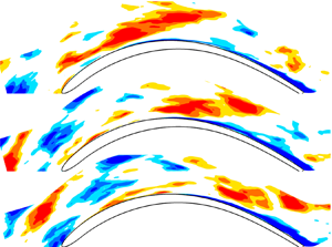
The magnitude of the velocity fluctuations in the passage seems to be linked to the generation of coherent structures in the blade boundary layers, which can be observed in the instantaneous perturbation velocity plots in figure 6. In the low FSTI case, the free stream region is weakly affected by the fluctuations. Here, the massively separated flow area is accompanied by the generation of large-scale KH rolls, as also shown in the experimental work of Lengani & Simoni (Reference Lengani and Simoni2015). Particularly, the separated shear layer can be seen in the rear part of the suction side just downstream of the position of the suction peak. The KH rolls are only generated close to the blade trailing edge as highlighted by the enlarged view on top right-hand side. Some structures can also be observed on the pressure side, just downstream of the separated flow area observed in figure 5. A completely different scenario characterizes the high FSTI case. The free stream region is affected by a dense population of structures of different sizes, and they appear randomly distributed in space in the whole passage. In the time instant shown in figure 6, a multitude of structures influence the flow around the leading-edge area. Free stream fluctuations are convected throughout the cascade passage, and they act as a continuous external forcing on the boundary layer over the suction side of the blade (please refer to the movie attached in the supplementary material available at https://doi.org/10.1017/jfm.2022.127). In the vicinity of the position of the suction peak, energetic low-speed structures can be observed inside the boundary layer (e.g. see the blue stripe close to the position marked with the letter ‘p’ in the panel). Breakdown of these structures causes transition upstream of the blade trailing edge (see the enlarged view in the top right-hand corner), which prevents the occurrence of the boundary layer separation. Inspection of the full movie (attached as supplementary material) gives insight into the complexity of the transition scenario in this high FSTI case.

Figure 6. Typical instantaneous flow field: (a) low FSTI; (b) high FSTI. The contour of streamwise velocity fluctuations and fluctuating velocity vectors  $(u',v')$ from the DNS. The enlarged view on top, related to the rear part of the blade suction side, identifies the structures affecting transition. The abbreviation ‘KH’ identifies a vortex related to the Kelvin–Helmholtz instability. The letter ‘p’ identifies the suction peak position.
In figure 7, a close-up view of two-dimensional slices in the wall-normal and wall-parallel planes are reported for the high FSTI case. The spatial position of these planes can be observed in figure 7(a). A typical snapshot is reported to show a view of the flow structures that populate the suction side boundary layer (a movie is provided in the supplementary material to give an idea of the dynamics at play). Alternating low- and high-speed bands of structures can be observed in the wall-parallel plane (figure 7d). They appear quite ordered in the bottom half of this plane, with shear effects acting in-between the low- and the high-speed filaments. The product  $u'w'$ is seen in the form of a localized vorticity region in the top half of the wall-parallel plane. Similarly, the panel on the right helps to identify the region characterized by high shear stress events that are formed at the edge of the low-speed regions (see the isolines of $u'=-0.4$). The wall-normal plane (figure 7b), taken in the middle of the wall-parallel plane, identifies low-speed regions. Intense ejection events (with instantaneous vectors pointing in the second quadrant according to Nolan, Walsh & McEligot (Reference Nolan, Walsh and McEligot2010)) may be observed. In this snapshot, high tangential negative Reynolds stresses, $u'v'$ (see also figure 7c), characterize the flow and seems to highlight breakup events that are characterized by shear stress events in both planes.

Figure 7. (a) Three-dimensional view of the blade with two-dimensional planes in the rear of the suction side: wall-normal plane (black); wall-parallel plane (red); cross-stream planes (blue). The planes are adopted for visualization purposes. Panels (b,d) are instantaneous snapshots in wall-normal (b) and wall-parallel (d) planes. The contour of streamwise velocity fluctuations and fluctuating velocity vectors  $(u',v')$ on (b) and $(u',w')$ on the (d) for the high FSTI case. Panels (c,e) are instantaneous $u'v'$ on (c) and $u'w'$ on (e), isocontour lines of $u'=-0.4$ are superimposed for completeness. (a) Reference planes; (b–e) typical snapshot.
4.2. POD analysis
In order to provide a clear statistical representation of the structures leading to transition in the high FSTI case, the classical version of POD has first been used to describe the modal contribution to the normal and the shear stresses in the different parts of the blade channel according to (3.2). The POD has been computed on 993 instantaneous flow field snapshots that have been sampled during 4.5 flow-through times. The convergence of POD modes has been checked with the approach of Hekmati, Ricot & Druault (Reference Hekmati, Ricot and Druault2011). Namely, different sets of POD modes have been computed by progressively increasing the number of snapshots that constitute the field matrix  $\boldsymbol {U}$. The convergence is given by the similarity of the modes between the different sets. It has been found that 800 snapshots are sufficient to reach the convergence on the first 50 modes. The first 200 modes are fully converged after including 95 % of the snapshots into the matrix.
The statistical representation of the fluctuating energy carried by each mode is provided in figure 8. This figure shows the normalized distribution of the cumulative sum of eigenvalues and their quota to the TKE production, on figure 8(a) and figure 8(b), respectively. The first 10 modes represent approximately 20 % of the TKE of the flow, and approximately 200 modes are necessary to capture 80 % of the total energy. Such dispersion of the POD eigenvalues indicates that the flow dynamics is ruled by highly stochastic events, which is typical of a free stream induced transition scenario (see also Liu et al. (Reference Liu, Adrian and Hanratty2001) and Lengani & Simoni (Reference Lengani and Simoni2015)). The distribution of the production of TKE integrated in the whole volume indicates a similar behaviour, where the first 200 modes also capture 80 % of the total  $P_{TKE}$. However, the analysis in the different integration volumes highlights that 200 modes capture all the information in the blade passage and in the blade boundary layer region. Interestingly, the POD identifies contribution to $P_{TKE}$ in the wake region just with high-order, less energetic modes. Therefore, since the modes related to the largest scale structures are able to better identify the turbulence production in the passage and boundary layer region, the following analysis will be limited to the most energetic mode. Figure 9 shows isosurfaces of the streamwise component of typical, high energetic modes (the first, the 7th and the 19th). These modes show elongated structures embedded into the suction side boundary layer. They appear downstream of the position of the suction peak, with a larger concentration in the trailing edge region. In the higher-order modes, structures appear evidently finer and even more concentrated on the trailing edge of the blade and also extending in the wake region. The most energetic modes are characterized by a large wavelength in the spanwise direction, while higher-order modes exhibit finer scales. In summary, all these modes highlight similar structures that are elongated in the streamwise direction, while their spanwise wavelength becomes smaller for higher-order modes. This consideration holds for all the modes that carry high energy and high $P_{TKE}$, whereas, as a consequence, we limit the analysis in this section to the visual inspection of the first mode only. The effect of the different spanwise wavelengths at hand will be quantified in the last section of the paper.

Figure 8. Cumulative contribution of each POD mode to the TKE (a) and its production (b) in different integration domains: (a) POD eigenvalues; (b)  $P_{TKE}$ captured.

Figure 9. Isosurface of streamwise component  $\phi _u$ of typical POD modes (1st, 7th and 19th). Blue and red isosurfaces identify negative and positive values ( ${\pm }0.03$), respectively.
The contribution of the first POD mode to the normal and shear components of the Reynolds tensor is reported in figure 10. Figure 10(a) shows the normal stress related to the streamwise fluctuations and provides the same results found in figure 9. The pattern shown by this quantity appears evidently ordered, without a trace of bursting events, similar to the first time instant previously discussed, referring to figure 7. However, this quantity is the only term of the Reynolds no stresses with high values on the blade suction side. In fact, no significant contributions of  $\phi _v^2$ and $\phi _w^2$ (figure 10b,c) can be observed on the whole suction side boundary layer.

Figure 10. Contribution to the Reynolds normal and shear stresses of the first POD mode. (a–c) Isosurfaces of partial  $\overline {u'^2}$; $\overline {v'^2}$ and $\overline {w'^2}$ (from left to right) are traced in red ( $0.001$). (d–f) Isosurfaces of partial $\overline {u'v'}$, $\overline {u'w'}$ and $\overline {v'w'}$ (from left to right) are traced in red and blue, indicating positive and negative contributions ( ${\pm }0.0005$), respectively. (a–c) Contribution to Reynolds normal stresses of first POD mode. (d–f) Contribution to Reynolds shear stresses of first POD mode.
The modal decomposition of the shear stress terms is reported for the same mode in figure 10(d–f). The isosurfaces, in this case, represent positive (red) and negative (blue) contributions to the corresponding shear stress term. The spatial distribution of the modal contribution to  $\overline {u'v'}$ in figure 10(d) highlights finer scale structures just in the rear part of the suction side. Wedge-shaped regions fed by coherent small-scale structures are clearly observable. The pattern of this modal distribution changes with respect to the normal components of the Reynolds stress shown in previous figures. The isocontour of $\phi _u\phi _v$ does not show a preferred direction for the elongation of structures. These events closely mark turbulent spots (Burgmann & Schröder Reference Burgmann and Schröder2008) and could be directly linked to the breakup events induced by the later stage of streak breakdown.
The contour plots of  $\phi _u\phi _w$ in figure 10(e) highlight again the occurrence of elongated filaments contributing to the shear stress in the rear part of the suction side. Interestingly, the spatial scale in the $z$ direction shown here is evidently smaller than the corresponding trace of the mode contributing to normal stress. Structures that are shown here still appear quite ordered (and decrease their wavelength for higher-order modes, similar to what was found in figure 9). These modal distributions provide a statistical representation of the shear effects in-between low- and high-speed filaments occurring in the wall-parallel plane previously observed in the instantaneous images of figure 7.
The contribution to  $\overline {v'w'}$ (figure 10f) on the suction side is smaller than that of the other two Reynolds shear stresses since the isosurfaces of $\phi _v\phi _w$ are not visible. The term $\phi _v\phi _w$ only marks activity on the pressure side. On the pressure side, the modal decomposition of the streamwise normal stress ( $\overline {u'^2}$) (figure 10a) is confined to the region just downstream of the leading edge. Conversely, $\phi _v^2$ and $\phi _w^2$ (figure 10b,c) clearly highlight large-scale structures on the pressure side of the blade. Figure 11 shows the spatial distribution of these quantities adopting a different field of view from the bottom of the blade. The POD mode highlights isosurfaces as elongated tubes preferably aligned with the streamwise direction, with a large wavelength in the spanwise direction. This scenario results from the normal stresses in the spanwise direction and the consequent shear stresses in the wall-normal direction. The breakups of the elongated structures observed on the pressure side are due to shear effects mainly acting in the cross-stream plane.

Figure 11. Contribution to the Reynolds normal ( $\phi _v^2$ and $\phi _w^2$) and shear ( $\phi _v\phi _w$) stresses of the first POD modes, blade pressure side view. Isosurfaces of partial $\overline {v'^2}$, $\overline {w'^2}$ and $\overline {v'w'}$ (from left to right) are traced in red and blue, indicating positive and negative contributions, respectively. The values of the isosurfaces are the same used in figure 10: $0.001$ for $\phi _v^2$ and $\phi _w^2$ and $\pm 0.0005$ for $\phi _v\phi _w$.
4.3. Extended POD analysis on temporal basis
The results in previous sections suggest that on the suction side, the modal decomposition of the different components of the Reynolds stress tensor can describe the different stages of transition, from the ordered pattern of streaky structures to the final stage of breakup and the resulting formation of randomized structures close to the trailing edge. However, such analysis cannot provide any information about the mechanisms leading to the initial stage of penetration/formation of such structures in the boundary layer. In order to investigate the role played by leading-edge receptivity and the continuous forcing from the passage region, results from extended POD are shown in this section. Extended POD modes presented here are the results of projecting the instantaneous snapshots on the temporal basis extracted from a limited portion of the passage and leading-edge domains (blue and red areas in figure 3, respectively).
Before focusing on the results regarding the blade boundary layers, figure 12 is introduced to provide a visualization of the structures identified by the extended POD procedure. Here, the first mode of the streamwise velocity ( $\phi _u$) is shown. In figure 12(a,b), the snapshot matrix has been projected on the first time coefficient ( $\chi ^1$) of the basis extracted in the leading edge region. This gives a comprehensive view of the spatial distribution of the modal representation correlating with the leading-edge events. Note that in this case, the mode is an extended mode for the area outside of the leading-edge region. Two different views of the blade are proposed in the figure to better highlight the turbulent field captured by this mode. Figure 12(a,b) shows large-scale structures at the inlet of the blade. The feature identified by figure 12(a) is a region of positive $\phi _u$ just in front of the blade leading edge. Figure 12(c,d) is obtained by projecting the snapshot matrix on the passage base. The passage base is defined in the rear part of the blade away from the blade surface (see the blue area of figure 3). Even though this base is extracted away from the leading edge, the figure shows large bulks of positive or negative values of $\phi _u$ at the inlet of the blade. Contrary to what is isolated by the leading-edge basis, these bulks are localized away from the leading edge.

Figure 12. Isosurface of the streamwise component  $\phi _u$ of the first POD modes of the extended POD. The mode is obtained by projecting the snapshot matrix on the leading-edge temporal base (a,b) and the passage temporal base (c,d). Light blue and yellow isosurfaces identify negative and positive values ( ${\pm }0.012$), respectively. To highlight the different structures identified by the two basis, two different views of same mode are shown; the one on the right is a rotated view to highlight the leading-edge region. (a,b) Leading-edge ‘basis’; (c,d) passage ‘basis’.
The relation between events embedded in the two bases with the structures on the blade boundary layer is discussed by means of the representation of the contributions to the Reynolds stress tensor provided by the extended POD projection (3.5). Results are shown for the first mode only since the behaviour of the higher-order modes is similar. As discussed in § 3.2, the correlation between the temporal basis of classical POD and that extracted from the limited portion on the leading edge and free-stream region gives a direct and quantitative estimation of correlation between the temporal events in these regions and the structures developing inside the boundary layer.
Figure 13 describes the spatial distribution of the first extended POD mode in terms of  $\phi _u^2$, $\phi _u\phi _v$ and $\phi _u\phi _w$. The modes are obtained by a projection of the classical POD temporal coefficient (i.e. extracted on the whole domain) on the temporal coefficient extracted from the leading-edge region (figure 13a–c) and from the passage (figure 13d–f), respectively. The streamwise normal stress obtained by a projection on the leading-edge basis leads to a modal representation highlighting finer scale structures in the rear part of the suction side with respect to classical POD (compare with figure 10a–c). The projection on the passage shows a similar representation, as made evident in figure 13(d–f). These results suggest that penetration and formation of streaky structures in the rear part of the blade suction side are due to both leading-edge receptivity and continuous forcing from the free stream. However, structures shown in figure 13(d–f) more closely resemble those shown in figure 10(a–c), thus providing the first evidence that the continuous forcing of turbulent structures from the passage is more related to transition events than to the leading-edge receptivity process.

Figure 13. Contribution to the Reynolds normal ( $\phi _u^2$) and shear ( $\phi _u\phi _v$ and $\phi _u\phi _w$) stresses of the first extended POD modes, blade suction side view. The mode is obtained by projecting the snapshot matrix on the leading-edge temporal base (a–c) and the passage temporal base (d–f). Isosurfaces are traced in red and blue, indicating positive and negative values, respectively. The contour level of the isosurfaces is the same of figure 10, (i.e. $0.001$ for contribution to normal and $\pm 0.0005$ for shear stresses). A larger isosurface corresponds to a large degree of correlation. (a–c) Leading-edge ‘basis’; (d–f) passage ‘basis’.
The extended POD projection of the  $\overline {u'v'}$ component is shown in figure 13(b,e). The spatial distribution in figure 13(a–c) suggests that breakup events are poorly correlated with the leading-edge related events. The correlation seems just slightly higher for the free stream oscillations (figure 13d–f). This is in agreement with the fact that structures on the suction side are forced by free stream/leading-edge perturbations, but their breakup (secondary instability, etc.) do not directly depend on those perturbations. This will be further discussed in the last section of the paper.
The extended POD modes for  $\phi _u\phi _w$ are presented in 13(c, f). This term may be linked to the initial stage of destabilization between high- and low-speed streaks inducing shear stress events, as also observed in figure 7. Projection on the leading-edge bases provides significant correlation only in the rear part of the suction side close to the blade trailing edge (figure 13a–c). A better correlation, which corresponds to a large isosurface, with a high value of the extended mode (see § 3.2), can be observed on the basis extracted from the passage. In figure 13(d–f) shear stress events in this plane can again be recognized in the whole decelerating part of the blade suction side, and they appear even upstream of what observed in figure 10(d–f).
A completely different scenario can instead be observed on the pressure side. Figure 14 shows the extended POD projections on the blade pressure side, adopting the same bottom view of figure 11. The normal and shear contributions to  $\overline {v'^2}$, $\overline {w'^2}$ and $\overline {v'w'}$ are shown from left to right in the figure. The elongated structures that are clearly visible in the classical POD modal representation in figure 11 are practically absent when projected on the leading-edge basis (figure 14a–c). A partial representation of them is instead found once projected on the passage temporal basis (figure 14d–f). Thus, such kind of structures that strongly resemble Görtler vortices do not seem to be affected by leading-edge receptivity and are linked to the continuous forcing from the passage region, mainly by means of normal stresses in the spanwise direction.

Figure 14. Contribution to the Reynolds normal ( $\phi _v^2$ and $\phi _w^2$) and shear ( $\phi _v\phi _w$) stresses of the first extended POD modes, blade pressure side view. The mode is obtained projecting on the leading-edge temporal base (a–c) and on the passage temporal base (d–f). Isosurfaces are traced in red and blue, indicating positive and negative values, respectively. The contour level of the isosurfaces is the same of figure 11, (i.e. $0.001$ for contribution to normal and ${\pm }0.0005$ for shear stresses). A larger isosurface corresponds to a large degree of correlation. (a–c) Leading-edge ‘base’; (d–f) passage ‘base’.
The degree of correlation of the coherent structures on the suction and pressure sides with perturbations in the leading edge and passage regions is quantified by the volume integral of the  $P_{TKE}$. The cumulative turbulent kinetic energy production for the classical POD and for different projected cases are shown in figure 15. The plots are normalized by the total TKE production inside the boundary layer over the blade. The optimal projection reaches the total cumulative value for a lower number of modes than the others. For the suction side, the projections on the passage and leading-edge basis show a similar degree of correlations for the first six modes. For the higher-order modes, the projection on the leading-edge base evidently reduces with respect to the projection on the passage. Thus, the cumulative curves in figure 15 make it evident that the correlation on the passage is higher than the correlation on the leading edge. On the pressure side, the structure projected on the leading-edge base do not produce TKE for the first six modes. The projection is evidently better on the passage base since higher $P_{TKE}$ is shown for every mode.

Figure 15. Cumulative contribution to the TKE production of classical and extended POD reconstructions on the suction (a) and pressure (b) side.
4.4. Extended POD analysis along the  $z$ direction

In order to present more detailed information on the characteristic wavelengths of the structures present in the suction side boundary layer, the POD has also been performed looking at coefficients in the  $z$ direction (3.4). The modes are represented in the $(x,y,t)$ plane, i.e. they provide the temporal evolution of the flow features in the $(x,y)$ physical space that are characterized by a spanwise wave according to their coefficient $\chi (z)$. Thus, they directly provide a view of the disturbance dynamics, from their penetration into the boundary layer to the final stage of the breakup, leading to the formation of shear stress events in the rear part of the blade. This analysis complements and merges all previous observations. The POD-z has been computed on limited domains: the leading edge and rear passage areas as defined in figure 3 as well as on the rear suction side area (i.e. the boundary layer region after the suction peak). Note that in the POD-z, the number of modes corresponds to the number of computational points along the spanwise direction and the convergence history differs from that of the classical POD procedure previously described. The cumulative distribution of the eigenvalues in the leading edge and the passage regions (figure 16) shows that convergence is achieved with 50 modes, and modes above 35 retain almost no energetic contribution. Therefore, the extended POD-z analysis is limited to these first 50 energetic modes. Conversely, on the rear suction side, there is a significant energetic contribution also for modes above 50. This is probably due to the breakdown into smaller spanwise wavelengths that are not present (or with negligible energy) in the free stream turbulence. In this latter case, the procedure of Hekmati et al. (Reference Hekmati, Ricot and Druault2011) has been applied to the POD-z modes to check the convergence. In this case, the spanwise extension has been kept fixed, and the number of points in the $z$ direction has been reduced. The modes up to the 50th are already well captured with half of the points.

Figure 16. Cumulative distribution of the POD-z eigenvalues in three different domains. Each distribution is normalized by the total energy in the respective domain.
The correlation matrix of the extended POD-z is computed as  $\boldsymbol {X}^{\rm T}_{V}\boldsymbol {X}_{\varOmega }$ (see also (3.6)) where the reference domain $V$ is the rear part of the suction side and the domains $\varOmega$ are alternatively the leading edge and the passage regions. Figure 17 shows the maximum degree of correlation between modes of these two regions (in the abscissa of the figure) with modes of the rear part of the suction side boundary layer. The values in the plots are quite high (above 0.4) for both regions. However, the highest degree of correlation is shown, almost for all modes, between the passage and the rear suction side regions, confirming what was discussed in the previous sections. The similarity between selected coefficients of these different domains and their characteristic spanwise wavenumber can be observed in figure 18. The POD coefficients in these plots are chosen among those with a degree of correlation above 0.8 and therefore show almost the same waveform in the two regions. The most energetic disturbance in the free stream ( $\hat {\beta }=7.24$) and disturbances belonging to the band predicted by the linearized theory ( $60<\hat {\beta }<200$) appear between those with a high degree of correlation between events occurring in the suction side and in the free stream. A mode exhibiting high correlation with a spanwise wavenumber in-between the most energetic and the optimal ( $\hat {\beta }=43.46$) is also shown. For what concerns the leading-edge region, only mode 5 with a spanwise wavenumber $\hat {\beta }=14.49$ is characterized by a degree of correlation higher than the free stream region, thus it is the only mode from the leading edge shown in figure 18(a). The other modes (figure 18b–f) are related to the passage region. The POD coefficients shown here strongly resemble Fourier modes due to homogeneity (in a statistical sense) in the $z$ direction. Amplitude modulation is limited for the low-order modes, and it appears more evident for mode 49, which is at the top of the band of the optimal disturbance.

Figure 17. Degree of correlation between modes of leading edge and passage regions with that of the rear suction side; only the maximum value is shown.

Figure 18. The POD coefficients computed in the different regions that have been considered for the extended POD-z analysis. These coefficients correspond to modes for which the degree of correlation is above 0.8 (see figure 17).
The r.m.s. of the streamwise component of POD-z modes, which have the maximum correlation, are shown in figure 19. These distributions are then compared with the gain predicted for the same spanwise wavenumber from optimal disturbance theory in figure 20. The results of figure 19 show that the most energetic disturbance of the free stream ( $\hat {\beta }=7.24$) is also responsible for the largest energy within the boundary layer. Interestingly, it grows similar to mode 5, which is correlated with the leading-edge region. Mode 5 is amplified downstream of $x/c=0.2$, while the disturbances correlating with the passage region are amplified downstream of $x/c=0.35$ (i.e. in the decelerating region of the suction side boundary layer). Summarizing, the fluctuations of the streamwise velocity induced by structures having large spanwise wavelength are correlated to events at both the leading edge and passage regions, further confirming what was found from figure 13.

Figure 19. Evolution of maximum root mean square (r.m.s.) of  $\phi _u$ within the blade suction side boundary layer.

Figure 20. Comparison of the maximum  $\phi _{u,rms}$ evolution within the boundary layer and optimal disturbance growth. The different curves have been normalized to unity at $x/c=0.35$.
Disturbances in the range of the optimal wavenumber ( $86.93<\hat {\beta }<173.85$) also grow significantly downstream of the position of the suction peak. The optimal disturbance analysis (figure 4) shows a very similar result for the spanwise wavenumber of interest. In fact, in the same range of $\hat {\beta }$ extracted from the extended POD-z, the optimal velocity amplification occurs mainly downstream of $x/c=0.35$. In order to provide a direct comparison between the optimal disturbance analysis and the growth of the r.m.s. of POD-z modes, data from POD and optimal theory have been normalized for the respective value at $x/c=0.35$ in figure 20. The two analyses present differences for the most energetic, low spanwise wavenumber mode. On the other hand, the optimal disturbance and POD-z agree well for the higher spanwise wavenumber corresponding to the most growing optimal disturbances (figure 20d–f).
The POD-z modes provide the temporal evolution of the structures in the  $(x,y)$ plane that are characterized by the spanwise wavenumber identified by the corresponding coefficients. For visualization purposes, three sequences of modes have been selected and shown in figures 21–23. The modes are obtained by projecting the velocity field on the $\chi (z)$ coefficients. The streamwise velocity of the mode is depicted in the sequence in panel (a), while the contribution to the partial Reynolds shear stress $\phi _u\phi _v$ is depicted in panel (b).

Figure 21. Temporal evolution of POD-z mode, distribution of modes of the streamwise velocity (sequence on panel (a)), distribution of partial shear stress  $\phi _u\phi _v$ on (b). The mode is obtained by projecting the whole velocity field on the POD coefficient of mode 5 computed from the leading-edge basis (figure 18a).
Figure 21 shows the spatial distribution of the extended POD mode of the leading-edge basis and its temporal evolution. The mode represented in the figure is the fifth, and it is characterized by a spanwise wavenumber of  $\hat {\beta }=14.49$ (see figure 18a). The wavenumber of this mode is almost twice that of the most energetic free stream disturbance and significantly smaller than the optimal one predicted by the linear theory. It is possible to observe the low and high streamwise velocity region from the sequence in figure 21(a). At the first instance, a negative velocity region (labelled with ‘A’ in the subpanel sequence) impacts the leading edge. Its trace and propagation are visible in the free stream region above and within the boundary layer. In the third time instant, this low-speed region is limited to the boundary layer region, and its intensity becomes bigger (smaller velocity), propagating downstream in the fourth and fifth subpanels of the sequence. This sequence confirms that a disturbance from the leading edge may propagate downstream as streamwise elongated structures with negative or positive disturbance velocity (see also figure 13). The sequence in figure 21(b) highlights that the Reynolds shear stresses related to the low (or high speed) region propagating from the leading edge have a very small amplitude. Particularly, the partial Reynolds shear stress related to the low-speed region previously identified is rather small, below the threshold defined in the figure. This further confirms the poor correlation between the structures that impinge on the leading edge and the breakdown process in the transitional region.
Figure 22 shows a similar scenario related to the most energetic free stream mode. The first subpanel of the sequence in figure 22(a) highlights a large region at high velocity (labelled with ‘B’ over the subpanel sequence) in the passage and boundary layer regions. This structure propagates downstream and retains a certain spatial coherence in the passage region above the boundary layer. A low-speed region in the boundary layer is also triggered close to the wall, just below the free stream perturbation (see the third and fourth subpanel of the sequence). Therefore, it confirms the link between region at a low (or high) velocity in the passage and response in the rear suction side boundary layer. Differently to what was observed in figure 21, the partial Reynolds shear stress captured by the mode sequence in figure 22 is not null in the region of the streamwise velocity perturbation: namely, negative  $\phi _u\phi _v$ appears in the last sequence in figure 22(b). Therefore, the projection on the passage base shows a certain degree of correlation with the breakup events identified by the Reynolds shear stress $\overline {u'v'}$. This is not the case for the projection on the leading-edge basis.

Figure 22. Temporal evolution of POD-z modes, distribution of modes of the streamwise velocity (sequence on panel (a)), distribution of partial shear stress  $\phi _u\phi _v$ on (b). The mode is obtained by projecting the whole velocity field on the POD coefficient of mode 1 computed from the passage basis (figure 18b).
The evolution of structures characterized by a spanwise wavenumber with  $\hat {\beta }=108.66$ is reported in the subpanel sequence of figure 23. This is representative of what happens for modes in the band of the optimum predicted by the linear theory. In this case, the regions of low and high speed inside the boundary layer and in the passage are considerably smaller than in the previous cases. Small perturbations propagate within the boundary layer; see, for example, the low speed region marked with ‘C’ in the first time snapshots. This low velocity region increases its magnitude moving downstream and triggers a region of growing negative Reynolds shear stress in the rear part of the blade boundary layer (see the sequence in figure 23b). Thus, even though characterized by significantly smaller energy, the evolution of the optimal disturbance in the suction side boundary layer correlates well with spanwise wave forced by the free stream, and it is responsible for the formation of shear stress events related to transition.

Figure 23. Temporal evolution of POD-z modes, distribution of modes of the streamwise velocity (sequence on panel (a)), distribution of partial shear stress  $\phi _u\phi _v$ on (b). The mode is obtained by projecting the whole velocity field on the POD coefficient of mode 31 computed from the passage basis (figure 18e).
5. Summary and conclusions
In the present work, analysis of DNS data shed further light on the role the free stream turbulence on the mechanisms leading to transition on both the pressure and the suction side of a low pressure turbine blade. Results account for the role played by the receptivity in the leading-edge region as well as the continuous forcing of free stream eddies at the boundary layer edge. Linear optimal disturbance analysis has been performed to identify the spanwise scale of the most amplified structures. Their evolution has been compared with that of the most energetic mode carried by the free stream and with that of other structures captured by POD.
Structures generated on the different parts of the blade have first been identified with POD, adopting its classical formulation. The POD modes provide a statistical representation of the structures contributing to both normal and shear stress. Ordered structures resembling streaky structures have been shown to mainly contribute to normal stress in the streamwise direction on the suction side. The shear stress between streamwise and spanwise directions ( $\phi _u\phi _w$) marks shear effects between the low- and high-speed streaks, while the shear between the streamwise and wall-normal direction ( $\phi _u\phi _v$) highlights breakup events. The pressure side is dominated by structures that are characterized by high normal stress in the spanwise and wall-normal directions and by their shear effects.
The extended POD formalism allowed us to quantify the correlation between the structures growing on both sides of the blade with the leading-edge related events and the forcing from free stream turbulence in the blade passage region. This first version of extended POD highlights the time-averaged correlating events between the boundary layer and the passage/leading-edge region. The events growing in the suction side boundary layer correlate better with the temporal basis describing the free stream oscillations in the passage. On the pressure side boundary layer, the degree of correlation with the passage region is even higher, while the correlation with the leading-edge basis is extremely poor. This implies that the leading-edge receptivity does not influence the generation and propagation of structures in the pressure side boundary layer.
The second variant of extended POD has been performed in the spanwise direction focusing on the results obtained in the suction side boundary layer. The extended POD-z provides the spatial evolution of the most energetic wavenumber carried by the free stream and allows comparison with the evolution of the optimal disturbance predicted by the linear theory. The region that correlates most with the events in the rear suction side is the passage, and, therefore, the free stream forcing seems to play a major role in the generation of structures in the boundary layer. The most energetic mode obtained by projection of the snapshot matrix on the leading-edge basis provides a limited contribution to the formation of shear stress events. On the other hand, the most energetic mode of the passage basis is clearly related to the generation of breakup events. Disturbances with spanwise wavenumbers in the optimal range show an amplification process in agreement with that predicted by the linear theory. These modes correlate mostly with the elements of the passage base, and once penetrated into the boundary layer, amplify in the rear suction side, inducing the breakup events responsible for the generation of the shear stress, thus transition.
Supplementary movies
Supplementary movies are available at https://doi.org/10.1017/jfm.2022.127.
Funding
The European Research Council provided financial support for this work under grant agreement 694452-TRANSEP-ERC-2015-AdG. The computations were performed on resources provided by the Swedish National Infrastructure for Computing (SNIC) at the PDC Center for High-Performance Computing at the Royal Institute of Technology (KTH) and the National Supercomputer Centre at Linköping University.
Declaration of interests
The authors report no conflict of interest.


 Open access