


1. Introduction
Two-layer flows of immiscible fluids with a heat source/sink along the interface are ubiquitous in natural and industrial settings (Levenspiel Reference Levenspiel1999; Bratsun & De Wit Reference Bratsun and De Wit2004; Gibson, Rosen & Stucker Reference Gibson, Rosen and Stucker2010; Ukrainsky & Ramon Reference Ukrainsky and Ramon2018; De Wit Reference De Wit2020). The presence of a heat source/sink along the interface could be due to a chemical reaction (Levenspiel Reference Levenspiel1999) or an irradiating beam along the liquid–liquid interface (Gibson et al. Reference Gibson, Rosen and Stucker2010). The chemical reactions cause a local change in the properties of the fluids such as density, viscosity, surface tension and elasticity, along with the temperature, due to the change in chemical composition and heat released/absorbed, which leads to an interplay between the reactions, hydrodynamics and heat transfer. Recent studies (De Wit, Eckert & Kalliadasis Reference De Wit, Eckert and Kalliadasis2012; Eckert et al. Reference Eckert, Acker, Tadmouri and Pimienta2012; De Wit Reference De Wit2016) on reactive systems show that this interplay then leads to various hydrodynamic instabilities such as Rayleigh–Taylor, viscous fingering, double-diffusive, and solutal or thermal Marangoni instabilities. Thus the resulting patterns in a reactive system are much more complex than in the corresponding non-reactive systems (De Wit Reference De Wit2020). Due to the immense importance of manipulating the rate of chemical reactions in industrial settings, understanding the dynamics of such reactive systems is essential.
Most of the previous studies, interestingly, assume reactive systems in the absence of an imposed shear and temperature fields (Bratsun & De Wit Reference Bratsun and De Wit2004; De Wit Reference De Wit2020). Thus any hydrodynamic flow or temperature field emerging in such systems will be a consequence of the chemical reactions alone. Bratsun & De Wit (Reference Bratsun and De Wit2004) considered an imposed shear and analysed reactive systems under restrictive assumptions, such as infinite liquid–liquid interfacial tension equivalent to an interface non-deformability, or flow in a Hele-Shaw cell that assumes no inertia. However, in many industrially and naturally important reactive systems, hydrodynamic flows generated by the imposed shear and temperature field coexist with a chemical reaction.
To understand such systems, a realistic model is necessary. For example, in batch and continuous stirred tank reactors, the shear force is employed to induce mixing to provide more contact area between the reacting chemical species (Levenspiel Reference Levenspiel1999). In tubular flow reactors, an axial pressure gradient causes the imposed shear flow (Levenspiel Reference Levenspiel1999). The present study attempts to fill this physically significant gap by considering a viscosity-stratified two-layer Couette flow with a heat source/sink along the interface.
Yih (Reference Yih1967) predicted the emergence of shear-wave instability in a two-layer Couette–Poiseuille flow as a result of the viscosity stratification. For the existence of the shear-wave instability, finite inertia and a deformable liquid–liquid interface are necessary. However, previous studies (Bratsun & De Wit Reference Bratsun and De Wit2004; De Wit Reference De Wit2020) concerning chemo-hydrodynamic instabilities assumed a non-deformable interface or the absence of the inertia, thereby missing the main ingredients for the shear-wave instability.
Wei (Reference Wei2006) analysed the stability of a two-layer Couette flow under an imposed temperature gradient across the bounding walls with the linear dependence of the interfacial tension on the temperature. He assumed that one of the layers is in the thin-film limit to proceed with the asymptotic analysis and governing equation derivation. The thin-film equations showed the presence of a non-local term which played an important role in determining the competition between the inertial and thermocapillary forces. His study showed an interesting interplay between the shear-wave and thermocapillary instabilities. However, the thin-film assumption (Wei Reference Wei2006) restricted the applicability of his study to the long-wave instabilities only, whereas finite-wave and short-wave instabilities remain to be investigated in a physically relevant system. Thermocapillary instabilities with heat generation along the non-deformable liquid–liquid interface in a stationary two-layer system was theoretically studied by Gilev, Nepomnyashchy & Simanovskii (Reference Gilev, Nepomnyashchy and Simanovskii1990) and Nepomnyashchy & Simanovskii (Reference Nepomnyashchy and Simanovskii2004). Their analysis demonstrated the presence of an oscillatory instability.
In the present paper, we consider a viscosity-stratified two-layer Couette flow with a heat source/sink along the interface, as shown schematically in figure 1. The liquid–liquid interface has a finite interfacial tension, which depends linearly on the temperature. The bounding walls are maintained at the same constant temperature, such that temperature gradients in the fluid layers may develop only due to the presence of the heat source/sink along the interface, unlike the case where an imposed temperature gradient was present only between the bounding walls (Wei Reference Wei2006). At the same time, the presence of a deformable interface along with a finite inertia leads to the emergence of the shear-wave instability. Thus the present study aims to investigate various instabilities arising as a result of an interplay between the inertial, viscous and thermocapillary stresses, and their impact on the stability of the system. It must be noted that, as shown in § 4, the stability characteristics of the system are not just a trivial superposition of shear-wave and thermocapillary instabilities but give rise to entirely new instabilities.

Figure 1. Schematic of the flow geometry in dimensional coordinates. The wall at  $y=R$ is moving with speed $V$ in the direction shown by the horizontal arrow. In the base state, the fluid–fluid interface located at $y=H R$, where the heat generation or absorption of intensity $Q$ takes place, separates the two liquids; $y=H R+h R$ is the location of the interface in the perturbed state, where $h R$ is the small displacement of the interface. Both bounding walls are held at the same dimensional temperature $T_0$.
The rest of the paper is arranged as follows. The base-state variables and governing equations for the perturbations are derived in § 2. The numerical method used here is discussed in § 3. The long-wave instability, the new instabilities and the associated critical parameters for streamwise perturbations are presented in § 4.1.1. The results for the finite-wave instability and the emerging neutral stability curves are presented in § 4.1.4. Instabilities of spanwise perturbations are studied in § 4.2. The physical mechanisms for the instabilities revealed in the paper are discussed in § 5. The salient conclusions of the paper are summarised in § 6.
2. Problem formulation
The system under consideration consists of two immiscible, incompressible Newtonian fluids confined between two horizontal planar walls, separated by the distance  $R$, as shown in figure 1. It is further assumed that the fluids extend infinitely in the lateral direction (along the $z$-axis). The two fluids, marked as $1$ and $2$, have different viscosities $\mu _1$ and $\mu _2$, respectively, but equal thermal conductivity $\kappa$, heat capacity $c_p$, and density $\rho$.
The Cartesian reference frame chosen here is such that its reference point is located on the lower substrate, the liquids flow in the  $x,z$-plane, and the $y$-axis is normal to the interface between the two layers at its undisturbed position located at $y=H R$. The upper wall moves in its plane with a dimensional steady velocity, $V$, whereas the lower wall is stationary. The lengths in the present problem are scaled by the channel spacing, $R$. The components of the velocity field are scaled by the speed of the wall, $V$, and the time $t$ is scaled by $R/V$. In the dimensionless coordinates, fluids $1$ and $2$ are confined to the domains $[0,H]$ and $[H,1]$, respectively, in the base state.
Due to the heat/source sink along the interface, a temperature gradient will develop across the fluid layers. To assign a definite sign to the Marangoni number and intensity of heat source/sink along the interface, we normalise the temperature with  $\beta _1 R$, where $\beta _1$ is the temperature gradient in fluid 1 in the base state. Both of the walls are held at the same dimensional temperature $T=T_0$. At the interface, heat generation or absorption takes place at a dimensionless rate $Q$, which may be either positive or negative, respectively, depending on whether a heat source/sink exists due to internal volumetric heat generation (Oron & Peles Reference Oron and Peles1998), or irradiation (Oron Reference Oron2000), as in the case of the photopolymerisation techniques used in additive manufacturing (Gibson et al. Reference Gibson, Rosen and Stucker2010).
The liquid–liquid interfacial tension,  $\sigma$, is assumed to be linearly temperature-dependent:
 \begin{equation} \sigma=\sigma_0-\gamma T, \end{equation}
where  $T$ is the local interfacial temperature, $\gamma =-{\rm d} \sigma /{\rm d}T>0$ and $\sigma _0$ is the reference interfacial tension of the fluid at an arbitrary reference temperature $T_r$. In what follows, all temperatures represent gauge temperatures with respect to $T_r$. This feature results in the emergence of Marangoni stresses at the interface, whenever a temperature variation along the interface exists, which may lead to thermocapillary instability.
We denote the velocity fields within the two fluids by  $\boldsymbol {v}^{(\boldsymbol {i})}=(v^{(i)}_x,v^{(i)}_y)$, where $i=1,2$ represent fluids $1$ and $2$, respectively. The dimensionless continuity equation is
 \begin{equation} \boldsymbol{\nabla} \boldsymbol{\cdot} \boldsymbol{v}^{(\boldsymbol{i})} =0, \end{equation}
where the gradient operator is  $\boldsymbol {\nabla }=\boldsymbol {e}_x \partial _ x+ \boldsymbol {e}_y \partial _ y$, with $\boldsymbol {e}_x$ and $\boldsymbol {e}_y$ denoting the unit vectors in the $x$- and $y$-directions, respectively. The dimensionless Navier–Stokes equations for the fluids with $\mu _1 V/R$ as the pressure scale are
 \begin{equation} Re\,[\partial_t \boldsymbol{v}^{(\boldsymbol{i})}+(\boldsymbol{v}^{(\boldsymbol{i})} \boldsymbol{\cdot} \boldsymbol{\nabla}) \boldsymbol{v}^{(\boldsymbol{i})}]={-}\boldsymbol{\nabla} p^{(i)} + \mu^{(i)}\,\nabla^{2} \boldsymbol{v}^{(\boldsymbol{i})}, \end{equation}
in which  $Re\equiv \rho V R/\mu _1$ is the Reynolds number and $\nabla ^2\equiv \partial _x^2+\partial _y^2$ is the Laplacian operator. The dimensionless viscosities are $\mu ^{(1)}=1$ and $\mu ^{(2)}=\mu _r$ for fluids $1$ and $2$, respectively, where
 \begin{equation} \mu_r =\frac{\mu_2}{\mu_1}. \end{equation}
Thus the dimensionless energy equations are
 \begin{equation} Pe\,[\partial_t T^{(i)}+(\boldsymbol{v}^{(\boldsymbol{i})} \boldsymbol{\cdot} \boldsymbol{\nabla}) T^{(i)} ]= \nabla^{2} T^{(i)}, \end{equation}
where  $Pe= Re\,Pr$ is the Péclet number and $Pr=\mu _1 c_p/\kappa$ is the Prandtl number based on the properties of fluid 1. Here the Prandtl number expresses the ratio of the kinematic viscosity (the momentum diffusivity) to the thermal diffusivity of liquid 1, whereas the Péclet number, $Pe\equiv \rho c_p V R/\kappa$, relates the rate of thermal convection to that of thermal diffusion in fluid 1.
The governing equations (2.2) are subjected to the following boundary conditions. Assuming no-slip, no-penetration and a constant specified temperature at the bounding walls yields
 $$\begin{gather} v^{(1)}_x=0, \quad v^{(1)}_y=0, \quad v^{(1)}_z=0, \quad T^{(1)}={\mathcal{T}}_0, \quad \text{at} \ y=0, \end{gather}$$
 $$\begin{gather}v^{(2)}_x=1, \quad v^{(2)}_y=0, \quad v^{(2)}_z=0, \quad T^{(2)}={\mathcal{T}}_0, \quad \text{at} \ y=1, \end{gather}$$
where  ${\mathcal {T}}_0$ is the dimensionless wall temperature.
The deformable fluid–fluid interface is assumed to be located at  $y= 1 +h(x,t)$, where $h(x,t)$ is the infinitesimal dimensionless displacement of the interface from its undisturbed position, ${y= 1}$. The boundary conditions at the interface are the kinematic boundary condition, and continuity of the tangential and normal components of the velocities and stresses, as well as continuity of the temperature and heat flux (Wei Reference Wei2005, Reference Wei2006), as follows:
 $$\begin{gather} \frac{\partial h}{\partial t} +v_x\,\frac{\partial h}{\partial x} = v_y, \end{gather}$$
 $$\begin{gather}\boldsymbol{v}^{(1)} - \boldsymbol{v}^{(2)} =0, \end{gather}$$
 $$\begin{gather}\boldsymbol{t} \boldsymbol{\cdot} \boldsymbol{\tau}^{(1)} \boldsymbol{\cdot} \boldsymbol{n} - \boldsymbol{t} \boldsymbol{\cdot} \boldsymbol{\tau}^{(2)} \boldsymbol{\cdot} \boldsymbol{n}={-} Ma\, \boldsymbol{\nabla} T \boldsymbol{\cdot} \boldsymbol{t}, \end{gather}$$
 $$\begin{gather}-p^{(1)} + \boldsymbol{n} \boldsymbol{\cdot} \boldsymbol{\tau}^{(1)} \boldsymbol{\cdot} \boldsymbol{n} - ({-}p^{(2)} + \boldsymbol{n} \boldsymbol{\cdot} \boldsymbol{\tau}^{(2)} \boldsymbol{\cdot} \boldsymbol{n})={-}Ca^{{-}1}\,(\boldsymbol{\nabla} \boldsymbol{\cdot} \boldsymbol{n}), \end{gather}$$
 $$\begin{gather}T^{(1)} - T^{(2)} =0, \end{gather}$$
 $$\begin{gather}\boldsymbol{\nabla} T^{(1)} \boldsymbol{\cdot} \boldsymbol{n} - \boldsymbol{\nabla} T^{(2)} \boldsymbol{\cdot} \boldsymbol{n} = Q {\mathcal{T}}_i, \end{gather}$$
where
 \begin{equation} Ma=\frac{\gamma \beta_1 H R}{\mu_1 V}, \quad Ca=\frac{\mu_1 V}{\sigma_0}, \quad Q=\frac{q R}{\kappa}. \end{equation}
Here,  $\boldsymbol {\tau }^{(\,j)}$ is the stress tensor in layer $j$,
$j$,  $Ma$,
$Ma$,  $Ca$ and $Q$ are the Marangoni number, the capillary number and the dimensionless heat source/sink intensity along the interface, respectively. The parameters $q$ and $\beta _1 = {{\rm d} \bar T_1 }/{{\rm d} y}$ are the dimensional heat source/sink intensity along the interface, and the base-state temperature gradient in fluid 1, respectively, with an overbar here and below denoting a base-state quantity. The vectors $\boldsymbol {t}$ and $\boldsymbol {n}$ represent the unit tangent and normal vectors to the free surface, respectively. The heat flux due to the interfacial heat source or sink is assumed to depend linearly on the temperature. To support this assumption, we note that the heat released/absorbed during a chemical reaction is proportional to the reaction rate and the enthalpy of the reaction, both of which are temperature-dependent (Levenspiel Reference Levenspiel1999). Therefore, to a first approximation, the heat released due to a chemical reaction is linear in the temperature with other parameters collectively represented here by the parameter $q$. It is noted that for an exothermic reaction $Q>0$, since heat is generated along the interface. The heat released at the interface increases the interfacial temperature, ${\mathcal {T}}_i$, raising it above the temperature of the bounding walls, ${\mathcal {T}}_0$. Thus the temperature gradient $\beta _1$ in fluid 1 will be positive, which implies $Ma>0$. Conversely, for an endothermic reaction, heat is absorbed along the interface, thus $Q<0$, and the interface will be at a temperature lower than that of the bounding walls so that $\beta _1 <0$ and $Ma<0$. The linearised expressions for the normal $\boldsymbol {n}$ and tangential vector $\boldsymbol {t}$ at the free surface, in the perturbed state, are
 \begin{equation} \boldsymbol{n}={-}\frac{\partial h}{\partial x}\,\boldsymbol{e}_{\boldsymbol{x}} + \boldsymbol{e}_{\boldsymbol{y}}, \quad \boldsymbol{t}=\boldsymbol{e}_{\boldsymbol{x}} + \frac{\partial h}{\partial x}\,\boldsymbol{e}_{\boldsymbol{y}}. \end{equation}
 The Marangoni number  $Ma$ can be rewritten as
 \begin{equation} Ma=\frac{\gamma \beta_1 H }{\mu_1 V/R}, \end{equation}
so that the term in the denominator,  $\mu _1 V/R$, denotes the viscous stress, whereas the term in the numerator, $\gamma \beta _1 H$, expresses the thermocapillary stress acting at the interface. Thus $Ma$ is a measure of the relative strength of the thermocapillary stresses compared to the viscous stresses. The dimensionless strength of the heat source/sink intensity at the interface, $Q$, is the ratio of the rate of heat generated/absorbed at the interface per unit area of the interface, $q$, to the rate of heat $\kappa /R$ conducted to (from) the interface from (to) the bounding walls. The capillary number $Ca$ can be rearranged to yield $Ca={(\mu _1 V/R)}/{(\sigma _0/R)}$, thus it can be interpreted as the ratio of viscous stresses ( $\mu _1 V/R$) to interfacial-tension stresses ( $\sigma _0/R$).
2.1. Base state
Assuming a steady, fully developed flow, the base-state equations are
 \begin{equation} \frac{{\rm d}^2 \bar v^{(i)}_x}{{{\rm d} y}^2}=0,\quad \frac{{\rm d}^2 \bar T^{(i)}}{{{\rm d} y}^2}=0, \end{equation}
subjected to the following boundary conditions. At the lower wall ( $y=0$),
 \begin{equation} \bar v^{(1)}_x = 0. \end{equation}
At the fluid–fluid interface ( $y=H$),
 $$\begin{gather} \bar v^{(1)}_x = v^{(2)}_x, \end{gather}$$
 $$\begin{gather}\frac{{\rm d} \bar v^{(1)}_x}{{\rm d} y} = \mu_r\,\frac{{\rm d} \bar v^{(2)}_x}{{\rm d} y}. \end{gather}$$
At the upper wall ( $y=1$),
 \begin{equation} \bar v^{(2)}_x = 1. \end{equation}
The solution of the above system of equations and boundary conditions (2.7) is
 \begin{equation} \bar v^{(1)}_x =\frac{\mu_r}{1+H(\mu_r-1)}\,y, \quad \bar v^{(2)}_x = \frac{H(\mu_r-1)}{1+H(\mu_r-1)} + \frac{1}{1+H(\mu_r-1)}\,y, \end{equation}
where an overbar indicates a base-state quantity. The base-state temperature gradients in the fluids are
 $$\begin{gather} \frac{{\rm d}\bar{T}^{(1)}}{{\rm d} y}=1, \quad \frac{{\rm d}\bar{T}^{(2)}}{{\rm d} y}=\frac{H}{H-1}, \end{gather}$$
 $$\begin{gather}\beta_1 = \frac{q T_0 (1 - H)}{\kappa+(H-1)HqR}. \end{gather}$$
The subsequent linear stability analysis is performed with respect to the base-state given by (2.8a,b) and (2.9a,b).
Note that in the case of no heat generation or absorption at the interface,  $q=0$, the temperature gradient $\beta _1$ is zero, therefore both $Q$ and $Ma$ vanish and the problem reduces to a purely isothermal one.
2.2. Linearised perturbation equations
For the purpose of the linear stability analysis, dynamic fields such as velocities, temperatures and pressures are represented by superposition of the base-state and the perturbations, as  $f(\boldsymbol {x},t)=\bar f(\boldsymbol {x},t)+f'(\boldsymbol {x},t)$. Here, $f(\boldsymbol {x},t)$ is a dynamic field and a prime denotes an infinitesimal perturbation. In the linearised governing equations, the normal modes take the form
 \begin{equation} f'(\boldsymbol{x},t)=\tilde{f}(y) \,{\rm e}^{{\rm i}(k x+m z - \omega t)}, \end{equation}
where  $k$ and $m$ are the streamwise and spanwise (real) wavenumbers, and $\tilde {f}(y)$ is the eigenfunction of $f'(\boldsymbol {x},t)$. The above normal modes are then substituted into (2.2) and (2.3). The parameter $\omega =\omega _r+ {\rm i} \omega _i$ is the complex frequency. Therefore, the flow is considered to be temporally unstable if at least one eigenvalue satisfies the condition $\omega _i>0$.
After substitution of the normal modes, the linearised governing equations become
 $$\begin{gather} {\rm i} k \tilde v^{(i)}_x + D \tilde v^{(i)}_y + {\rm i} m \tilde v^{(i)}_z=0, \end{gather}$$
 $$\begin{gather}Re\,[ -{\rm i} \omega \tilde v^{(i)}_x + {\rm i} k \bar v^{(i)}_x \tilde v^{(i)}_x + \tilde v^{(i)}_y\,D \bar v^{(i)}_x ] ={-}{\rm i} k \tilde p^{(i)} + \mu^{(i)} (D^{2}-k^{2}-m^2) \tilde v^{(i)}_x, \end{gather}$$
 $$\begin{gather}Re\,[ -{\rm i} \omega \tilde v^{(i)}_y + {\rm i} k \bar v^{(i)}_x \tilde v^{(i)}_y ] ={-}D \tilde p^{(i)} + \mu^{(i)} (D^{2}-k^{2}-m^2) \tilde v^{(i)}_y, \end{gather}$$
 $$\begin{gather}Re\,[ -{\rm i} \omega \tilde v^{(i)}_z + {\rm i} k \bar v^{(i)}_x \tilde v^{(i)}_z ] ={-}{\rm i}m \tilde p^{(i)} + \mu^{(i)} (D^{2}-k^{2}-m^2) \tilde v^{(i)}_z, \end{gather}$$
 $$\begin{gather}Re\,Pr [ -{\rm i} \omega \tilde T^{(i)} + D \bar T^{(i)}\,\tilde v^{(i)}_y ] = (D^{2}-k^{2}-m^2) \tilde T^{(i)}, \end{gather}$$
where  $D={\rm d}/{{\rm d} y}$. Equations (2.12) are subject to the following boundary conditions. At $y=0$ and $y=1$, the assumption of no-slip, no-penetration and constant temperature at the walls yields
 $$\begin{gather} \tilde v^{(1)}_x =0, \quad \tilde v^{(1)}_y =0, \quad \tilde v^{(1)}_z =0, \quad \tilde T^{(1)} =0, \quad \text{at} \ y=0, \end{gather}$$
 $$\begin{gather}\tilde v^{(2)}_x =0, \quad \tilde v^{(2)}_y =0, \quad \tilde v^{(2)}_z =0, \quad \tilde T^{(2)} =0, \quad \text{at} \ y=1. \end{gather}$$
At  $y=H$, oscillations of the fluid–fluid interface will be induced due to the perturbations. Thus the infinitesimal displacement of the interface will matter. These boundary conditions, after substitution of the normal modes, become
 $$\begin{gather} {\rm i} (k \bar v^{(1)}_x -\omega) \tilde h = \tilde v^{(1)}_y, \end{gather}$$
 $$\begin{gather}\tilde v^{(1)}_y = \tilde v^{(2)}_y, \end{gather}$$
 \begin{gather}\tilde v^{(1)}_x + D\bar{v_x}^{\!\!(1)}\,\tilde h = \tilde v^{(2)}_x + D\bar{v_x}^{\!\!(2)}\,\tilde h, \end{gather}
 \begin{gather}D \tilde v^{(1)}_x + {\rm i}k \tilde v^{(1)}_y={-} {\rm i}k\,Ma\,(\tilde T^{(1)} + D\bar T^{(1)}\, \tilde h ) + \mu_r ( D \tilde v^{(2)}_x + {\rm i}k \tilde v^{(2)}_y), \end{gather}
 $$\begin{gather}D \tilde v^{(1)}_z + {\rm i}m \tilde v^{(1)}_y={-} {\rm i}m\,Ma\,(\tilde T^{(1)} + D\bar T^{(1)}\, \tilde h ) + \mu_r ( D \tilde v^{(2)}_z + {\rm i}m \tilde v^{(2)}_y), \end{gather}$$
 $$\begin{gather}-\tilde p^{(1)} + 2 D v^{(1)}_y ={-}\tilde p^{(2)} + 2 \mu_r D v^{(2)}_y - Ca^{{-}1} k^2 \tilde h, \end{gather}$$
 $$\begin{gather}\tilde T^{(1)} + D\bar{T}^{(1)}\,\tilde h = \tilde T^{(2)} + D\bar{T}^{(2)}\,\tilde h, \end{gather}$$
 $$\begin{gather}D\tilde T^{(1)} = D \tilde T^{(2)} + Q ( \tilde T^{(1)} + D\bar T^{(1)}\,\tilde h ), \end{gather}$$
where all quantities are evaluated at  $y=H$.
3. Numerical method
To carry out the linear stability analysis of the problem (2.12)–(2.13), the pseudospectral method is employed, in which the eigenfunctions corresponding to each dynamic field are expanded into series of the Chebyshev polynomials. The Chebyshev polynomials are defined over  $[-1,1]$ while the domains of fluid 1 and fluid 2 are $[0,H]$ and $[H,1]$, respectively. Thus, for discretisation, we use the substitutions
 $$\begin{gather} y \rightarrow \frac{H}{2}(1+y), \quad \text{for fluid 1}, \end{gather}$$
 $$\begin{gather}y \rightarrow \frac{1}{2}(1+H+(H-1)y), \quad \text{for fluid 2}, \end{gather}$$
mapping the domains for fluid 1 and fluid 2 onto  $[-1,1]$ and $[1,-1]$, respectively. The eigenfunctions are further expanded in terms of the transformed coordinate as
 \begin{equation} \tilde{f}(y)=\sum_{m=0}^{m=N} a_m\,{\mathcal{C}}_m (y), \end{equation}
where  ${\mathcal {C}}_m(y)$ are Chebyshev polynomials of degree $m$ and $N$ is the highest degree of the polynomial in the series expansion or, equivalently, the number of collocation points. The coefficients of the series $a_m$ are the unknowns to be solved for.
The generalised eigenvalue problem is constructed in the form
 \begin{equation} \boldsymbol{\mathsf{A}}\boldsymbol{e} + c \boldsymbol{\mathsf{B}}\boldsymbol{e}=0, \end{equation}
where  $\boldsymbol{\mathsf{A}}$ and $\boldsymbol{\mathsf{B}}$ are matrices obtained from the discretisation procedure and $\boldsymbol {e}$ is the vector containing the coefficients of all series expansions.
Further details of the discretisation of the governing equations and boundary conditions, and the construction of the matrices  $\boldsymbol{\mathsf{A}}$ and $\boldsymbol{\mathsf{B}}$, are presented in the standard procedure described by Trefethen (Reference Trefethen2000) and Schmid & Henningson (Reference Schmid and Henningson2001). Application of the pseudospectral method for similar problems can be found in Patne, Agnon & Oron (Reference Patne, Agnon and Oron2020, Reference Patne, Agnon and Oron2021). We use the polyeig MATLAB routine to solve the generalised eigenvalue problem given by (3.4). To filter out the spurious modes from the genuine, numerically-computed spectrum of the problem, the latter is determined for $N$ and $N+2$ collocation points, and the eigenvalues are compared with an a priori specified tolerance, e.g. $10^{-4}$. The genuine eigenvalues are verified by increasing the number of collocation points by $25$ and monitoring the variation of the obtained eigenvalues. Whenever the eigenvalue does not change up to a prescribed precision, e.g. to the sixth significant digit, the same number of collocation points is used to determine the critical parameters of the system. In the present work, $N=50$ is found to be sufficient to achieve convergence and to determine the leading, most unstable eigenvalue within the investigated parameter range. The numerical method employed here to solve the eigenvalue problem is validated in figure 2 by comparing the growth rate predicted by the present numerical approach and the data points from Shankar & Kumar (Reference Shankar and Kumar2004).

Figure 2. Variation in the growth rate  $c_i$ with wavenumber $k$ for $Re=1$, $H=0.4$, $\mu _r=0.5$, $Pe = 0$, $Ma=0$, $Q=0$ and $Ca=100$ predicted by the present numerical approach and Shankar & Kumar (Reference Shankar and Kumar2004). The figure illustrates excellent agreement between the results of the numerical computation and digitally extracted data points from figure 3(a) of Shankar & Kumar (Reference Shankar and Kumar2004), thereby validating the former.
In the limit of small Péclet number, i.e.  $Pe \equiv Re\,Pr = 0$ and $m=0$, the energy equations for the fluids can be solved analytically to obtain
 $$\begin{gather} \tilde T^{(1)} = 2 m_1 \sinh (ky), \end{gather}$$
 $$\begin{gather}\tilde T^{(2)} ={-} 2m_2 \, {\rm e}^{k} \sinh (k-ky), \end{gather}$$
where  $m_i$ are the integration constants, and boundary conditions (2.13a) and (2.13b) have been used. The Orr–Sommerfeld equations for the fluids are numerically integrated by taking an initial guess value for $c$ to obtain the eigenfunctions for velocities:
 $$\begin{gather} \tilde v_x^{(1)} = m_3 v_{x1}^{(1)} + m_4 v_{x2}^{(1)}, \end{gather}$$
 $$\begin{gather}\tilde v_x^{(2)} = m_5 v_{x1}^{(2)} + m_6 v_{x2}^{(2)}, \end{gather}$$
where  $v_{x1}^{(1)}$, $v_{x2}^{(1)}$, $v_{x1}^{(2)}$ and $v_{x2}^{(2)}$ are the integrated velocity eigenfunctions.
The eigenfunctions (3.5) are then substituted in the interface boundary conditions (2.13). Thus we have six integration constants and six linear algebraic equations. In matrix form, the resulting eigenvalue problem becomes
 \begin{equation} \boldsymbol{\mathsf{M}} \boldsymbol{\alpha}=0, \end{equation}
where  $\boldsymbol{\mathsf{M}}$ is a $6 \times 6$ matrix containing the coefficients of the integration constants in (3.5), and $\boldsymbol {\alpha }$ is a vector containing the six integration constants $m_i$. The eigenvalue $c$ is then obtained by solving for the value of $c$ at which the determinant of the matrix $\boldsymbol{\mathsf{M}}$ vanishes, thereby determining the system stability. Next, the Newton–Raphson algorithm is utilised to obtain the initial guess for the next iteration. The obtained eigenvalues in each iteration are compared with an a priori specified tolerance, e.g. $10^{-6}$. Typically, an eigenvalue converges within $10$ iterations.
4. Results and discussion
Before proceeding with the presentation of the results, typical ranges of the dimensional and dimensionless parameters are presented in table 1. Note that  $Q$ and $Ma$ can assume positive or negative signs depending on whether a heat source or sink is present along the interface. These parameter ranges will be used here to study the various modes of instability. For the ease of presentation and discussion, the results have been divided into two sections, dealing separately with the streamwise ( $m=0$) and spanwise ( $k=0$) modes of instability.
Table 1. The magnitude of dimensional and dimensionless parameter ranges for the relevant processes considered in the present study (Li, Xu & Kumacheva Reference Li, Xu and Kumacheva2000; Schatz & Neitzel Reference Schatz and Neitzel2001; Ukrainsky & Ramon Reference Ukrainsky and Ramon2018).

4.1. Streamwise perturbation
The presence of a heat source along the interface,  $Q>0$, leads to an increase in the interfacial temperature relative to the bounding walls. This results in a positive temperature gradient in fluid 1, $\beta _1>0$, corresponding to $Ma>0$. The growth-rate curves $c_i(k)$ for the case of a heat source along the interface are shown in figures 3(a) and 3(b). A similar argument for the case of a heat sink along the interface leads to the conclusion that $Ma<0$ and $Q<0$. The corresponding growth-rate curves for the case of a heat sink along the interface are shown in figures 3(c) and 3(d).

Figure 3. Variation in the growth rate  $c_i$ with the disturbance wavenumber $k$ at $Re=10$, $H=0.4$, $\mu _r=0.5$, $Pe=0$, $Q=2$ and $Ca=0.1$ for the streamwise perturbations. Panels (a) and (b) are for the case of a heat source along the interface, i.e. $Q>0$ and $Ma>0$, illustrating the stabilising effect of a heat source along the interface on the pure shear-wave instability corresponding to $Q=Ma=0$. Panels (c) and (d) are for the heat sink along the interface, i.e. $Q<0$ and $Ma<0$, illustrating the destabilising effect of a heat sink along the interface on the pure shear-wave instability corresponding to $Q=Ma=0$. (a,c) The entire wavenumber domain. (b,d) The blowup of the low-wavenumber domain. The flow is unstable for $c_i>0$.
In figure 3, the curves for  $Ma=0$, $Q=0$ correspond to the pure shear-wave instability first revealed by Yih (Reference Yih1967) in the absence of the heat source/sink at the interface. The growth-rate curves illustrate the stabilising (destabilising) effect of the heat source (sink) along the interface on the pure shear-wave instability.
One might expect that a heat source that generates energy at the interface would lead to an enhancement of the shear-wave instability by providing energy to the perturbations with the opposite expectation for the heat sink. However, as discussed in § 5, the heat sink sets up a favourable arrangement for the thermocapillary instability by lowering the temperature of the interface with respect to the bounding walls. On the other hand, the heat source increases the temperature of the interface, thereby promoting an unfavourable set-up for the thermocapillary instability. This leads to the stabilisation or destabilisation of the pure shear-wave instability shown in figure 3, which demonstrates two types of instability modes, namely, the long-wave ( $k<0.1$) and the finite-wave ( $k>0.1$). For the convenience of the presentation, we separate the results into two subsections; the first analyses the long-wave mode, whereas the second deals with the finite-wave mode.
4.1.1. Long-wave instability
The long-wave streamwise instability is amenable to an asymptotic analysis. Before proceeding with the analysis, we substitute  $\omega =kc$ and write the system of two Orr–Sommerfeld equations obtained for the two fluids in the form
 \begin{equation} {\rm i}k\,Re\,( \bar v_x^{(i)} - c ) ( D^2 - k^2 ) \tilde v_y^{(i)} = \mu^{(i)}( D^2 - k^2 )^2 \tilde v_y^{(i)}, \end{equation}
where  $c=c_r+{\rm i}c_i$ is the complex phase speed. The energy equations remain unchanged. Next, the velocity and temperature fields, and the complex phase speed $c$, are expanded as series in terms of a small wavenumber $k$, as
 $$\begin{gather} \tilde v_y^{(i)}= v_{y0}^{(i)} + k v_{y1}^{(i)} + k^2 v_{y2}^{(i)} +\cdots, \end{gather}$$
 $$\begin{gather}c=c_0 + k c_1 + k^2 c_2 +\cdots, \end{gather}$$
 $$\begin{gather}\tilde T^{(i)}= \frac{1}{k} T_{0}^{(i)} + T_{1}^{(i)} + k T_{2}^{(i)} +\cdots. \end{gather}$$
These expansions are then substituted into the Orr–Sommerfeld equation (4.1), the energy equation (2.12e), and the boundary conditions (2.13).
At  $O(1)$, the governing equations read
 \begin{equation} D^4 v_{y0}^{(i)} = 0, \quad D^2 T_{0}^{(i)} = 0. \end{equation}
It must be noted that the corresponding expansions in powers of  $k$ for $\tilde v_x^{(i)}$ can be obtained via that for $\tilde v_y^{(i)}$ if needed, from the continuity equations, whereas the expansion for $\tilde p^{(i)}$ can be obtained from the $x$-component of the momentum equation.
Using the obtained expansions yields
 \begin{equation} c_0 = \frac{\mu_r H [1 + H (\mu_r - 1) (2 - 2 H + 2 H^2 + H^3 (\mu_r - 1))]} {(\mu_r -1)[1 + H (\mu_r -1)][1 + H (\mu_r - 1) (4 - 6 H + 4 H^2 + H^3 \mu_r - H^3)]}. \end{equation}
The  $O(1)$ eigenvalue, $c_0$, i.e. the wave celerity, is independent of $Q$, representing the intensity of the heat source/sink, or $Ma$, reflecting the relative importance of surface tension variation compared with shear stresses. It depends on the thickness ratio $H$ and the viscosity ratio $\mu _r$. For $H=0.4$ and $\mu _r=0.5$, (4.6) yields $c_0 = 0.31447$, in agreement with Shankar & Kumar (Reference Shankar and Kumar2004), serving as validation of our analysis at this point.
At  $O(k)$, the governing equations are
 $$\begin{gather} \mu^{(i)}\,D^4 v_{y1}^{(i)} + {\rm i}\,Re\,( c_0 - \bar v_{x}^{(i)} )\,D^2 v_{y0}^{(i)} = 0, \end{gather}$$
 $$\begin{gather}D^2 T_{1}^{(i)} + {\rm i}\,Pe\,( c_0 - \bar v_{x}^{(i)} ) T_{0}^{(i)} - Pe\,D \bar T^{(i)}\, v_{y0}^{(i)} = 0. \end{gather}$$
Solving (4.8) in the same way as for  $O(1)$ above, yields
 \begin{equation} c_1={\rm i}\left( \frac{ f_1 (H,\mu_r)\,Ma }{Q + f_3 (H)} + f_2 (H,\mu_r)\,Re \right). \end{equation}
Since  $c_1$ is purely imaginary, it represents the growth rate of perturbations with respect to the disturbance wavenumber and the rest of the parameters.
Combining (4.6) and (4.9), the eigenvalue  $c$, at $O(k)$, is
 \begin{equation} c=c_0(H,\mu_r)+{\rm i} k \left( \frac{ f_1 (H,\mu_r)\,Ma }{Q + f_3 (H)} + f_2 (H,\mu_r)\,Re \right), \end{equation}
where
 \begin{equation} f_1 =\frac{g_4}{g_5}, \quad f_2 = \frac{g_1 g_2}{g_3}, \quad f_3 = \frac{1}{H(H-1)}, \end{equation}
and
 \begin{align} \left.\begin{array}{c@{}} g_1 ={-}(H-1)^2 H^2 ( \mu_r - 1) [{-}1 + ({-}6 H^2 + 8 H^3 + 3 H^4 ( \mu_r - 1) -4 \mu_r ) ( \mu_r - 1)],\\ g_2 = 2 (H-1)^5 (2 H - 5 H^2 + H^3 ) \mu_r +8 (H-1)^2 H^2 ({-}1 + 2 H) (1 - H + H^2) \mu_r^2\\ \hspace{-2cm}{}- 2 (H-1) H^5 ({-}2 + 3 H + H^2) \mu_r^3 + H^8 \mu_r^4 -(H-1)^8,\\ g_3 = 60 H (H-1) [1 + H (\mu_r - 1)]^2 [1 +H (\mu_r - 1) (4 - 6 H + 4 H^2 + H^3 (\mu_r - 1))]^3,\\ g_4=(H-1) H^2 (2 H-1) [{-}1 + 2 H + H^2(\mu_r-1)],\\ g_5 = 2 + 2 H (\mu_r-1) [4 - 6 H + 4 H^2 + H^3 (\mu_r-1)]. \end{array}\right\} \end{align}
Interestingly,  $f_1 (H,\mu _r)$, representing the coefficient of $Ma$, and thus representative of the thermocapillary stresses along the interface, is a function of the viscosity ratio $\mu _r$ and the thickness ratio $H$. The former suggests a coupling between the thermocapillary and viscous stresses at the interface, which, as discussed below, strongly affects the stability of the system. The function $f_2$ is associated with the case of a pure viscous-stratification instability and, similar to $f_1$, depends on the viscosity and thickness ratios. It follows from (4.10) and (4.11a–c) that the long-wave mode is independent of $Pe$ and $Ca$, thus the results presented for the long-wave mode are valid for arbitrary $Pe$ and $Ca$; henceforth their values will not be specified when the long-wave mode is concerned.
The variation in the functions  $f_1 (H,\mu _r)$, $f_2 (H,\mu _r)$ and $f_3 (H)$ with parameters $H$ and $\mu _r$ is shown in figure 4. It is interesting to note that both $f_1$ and $f_2$ vanish at $H=0.5$ for any $\mu _r$. In the context of the instability threshold of the base state, this means that the state of the system for which $H=0.5$ is neutrally stable in terms of the long-wave instability. Figure 4(a) presents the variation in $f_1$ and $f_2$ with $H$ for $\mu _r=0.5$. Note $f_1$ has two zeros in the relevant domain of $0 < H<1$. Thus, for these two values of $H$, the thermocapillary stresses do not affect the stability of the system. It is seen that $f_2 > 0$ for $H<0.5$, whereas for $H>0.5$, $f_2$ is negative. These domains correspond, respectively, to the unstable and stable configurations for the shear-wave instability, first shown by Yih (Reference Yih1967). Also, $f_1$ is positive except for a short interval in $H$. In particular, $f_1<0$ for $0.5< H<0.6$, where $f_2 <0$. Thus, as will be seen below, even if the inertial terms (i.e. the terms with $Re$) are stabilising, and the shear-wave instability does not set in, the thermocapillary terms can induce instability via heat generation at the interface. Figure 4(b) presents the variation of the function $f_3$, which is always negative and independent of $\mu _r$. Figure 4(c) shows the variations in $f_1$ and $f_2$ with $\mu _r$ when the value of $H$ is fixed to a sample value of $H=0.4$, which will be used hereafter. Figure 4(d) presents the variation of $f_1$ and $f_2$ with $H$, for $\mu _r=1.5$. Note the change in sign of $f_2$ as compared to figure 4(a). The sign of $f_2$ is associated with the stability properties of the isothermal Couette flow in a two-layer system. Thus the effect of inertia exerted on the flow considered in this paper will be destabilising for a pair $(H, \mu _r)$ with $H<1/2$, $0< \mu _r <1$ or $H>1/2$, $\mu _r >1$; otherwise, it is stabilising.

Figure 4. Variation in the functions  $f_1(H,\mu _r)$, $f_2(H,\mu _r)$ and $f_3(H)$ with the relative position of the liquid–liquid interface $H$ and the viscosity ratio $\mu _r$. (a) Functions $f_1$ and $f_2$ for $\mu _r=0.5$. (b) Function $f_3$ for arbitrary $\mu _r$. (c) Functions $f_1$ and $f_2$ for $H=0.4$. (d) Functions $f_1$ and $f_2$ for $\mu _r=1.5$. The thin horizontal lines mark the zero values for $f_1$ and $f_2$.
In the absence of the heat source/sink along the interface, the temperature gradient in the fluids will vanish, in which case  $Ma=0$, $Q=0$, removing the thermocapillary effect in (4.10) and retaining only the shear-wave instability. For $H=0.4$ and $\mu _r = 0.5$, the shear-wave mode has
 \begin{equation} c=0.31447+ 1.2 \times 10^{{-}4} {\rm i}k\,Re, \end{equation}
in agreement with the results of Shankar & Kumar (Reference Shankar and Kumar2004), thus validating the results of our asymptotic analysis. The validity of the long-wave asymptotic analysis is further demonstrated in figure 5, through a comparison with the numerical results. At low  $k$, both approaches are in agreement, as expected from the long-wave expansion. At a finite $k$, there exists an additional mode of instability that is not captured by the long-wave asymptotic analysis, which we refer to hereafter as a ‘finite-wave instability’.

Figure 5. Variation in the growth rate  $c_i$ with wavenumber $k$ for $Re=10$, $H=0.4$, $\mu _r=0.5$, $Pe=0$ and $Ca^{-1}=0$ in the case of a heat source along the interface for the streamwise perturbations. The figure illustrates the excellent agreement between the results of the numerical computation and those of the long-wave asymptotic analysis, given by (4.10) at low $k$.
$k$.
4.1.2. Heat source along the interface
It follows from (4.10) that the Prandtl and capillary numbers do not affect the long-wave mode at first order in  $k$. For a heat source, representing an exothermic reaction along the interface, $Q>0$, $Ma>0$. In this case, as noted above, the thermocapillary stresses stabilise the shear-wave instability. Thus, at a fixed value of the other parameters, an increase in $Ma$ leads, in general, to the suppression of the shear-wave instability and the formation of stable and unstable domains in the parameter space. These domains are shown in figure 6 for typical values of $Q$,
$Q$,  $\mu _r$ and $Re$.
$Re$.

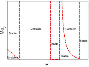
Figure 6. Variation of the critical Marangoni number  $Ma_c$ with the position of the liquid–liquid interface, $H$, at $Re=10$ for the streamwise perturbations due to interfacial heat source $Q$. At $H=0.5$, $f_1=0$, so thermocapillarity does not affect the stability. (a) $Q=0.1$, $\mu _r=0.5$; (b) $Q=6$, $\mu _r=0.5$; (c) $Q=0.1$, $\mu _r=1.5$; (d) $Q=6$, $\mu _r=1.5$. (a,c) Stabilisation introduced by thermocapillarity due to a heat source along the interface. (b,d) Explosive and interaction instabilities introduced by the heat source along the interface. (a) For $0.5< H<0.6$, thermocapillarity causes the emergence of the interaction instability. (b) The interaction between the viscous stratification and thermocapillarity leads to the emergence of a stable patch in $0.5< H<0.6$ and of the explosive instability for $0.21 \lesssim H \lesssim 0.5$. (d) The interaction between the viscous stratification and thermocapillarity leads to the emergence of a stable patch in $0.2 < H <0.5$ and the explosive instability in $0.5 < H \lesssim 0.78$.
The two values of  $\mu _r$ are selected such that fluid 1 has either higher ( $\mu _r<1$) or lower ( $\mu _r>1$) viscosity than fluid 2. Solving the neutral stability equation ( $c_i=0$) based on (4.10) in terms of $Ma$ yields the critical value
 \begin{equation} Ma_c={-}\frac{[Q + f_3 (H)]\, f_2 (H,\mu_r)\,Re}{ f_1 (H,\mu_r) }, \end{equation}
which shows that a variation in  $Re$ will have a simple multiplicative effect on the critical value of $Ma$, while preserving the qualitative features of the marginal stability curves. In the present analysis, $Re>1$ has been chosen deliberately to provide clarity in the subsequent figures. As for $Q$, the two chosen values are such that for one of them $Q<-f_3$ for all $H \in [0,1]$, while for the other value, $Q> -f_3$ for a range of $H$ indicated in the corresponding figures.
Figure 6(a) illustrates the stabilising effect imparted by the presence of the heat source on the shear-wave instability emerging when  $H<0.6$. For $H>0.6$, the shear-wave mode is stable, thus thermocapillary stresses, stabilising in this case, do not have any qualitative effect. Interestingly, at $H=0.5$, the coefficient of $Ma$,
$Ma$,  $f_1$, vanishes when $\mu _r = 0.5$, so that thermocapillary stresses do not have any effect on the instability. Under such conditions, the asymptotic expression (4.10) reduces to
 \begin{equation} c=0.41414+ 2.85994 \times 10^{{-}6} {\rm i}k\,Re,\end{equation}
in which the Marangoni term is absent. For  $0.5< H<0.6$, both $f_1$ and $f_2$ are negative. In fact, the function $f_2$ is expected to be negative, in agreement with previous work (Yih Reference Yih1967; Charru & Hinch Reference Charru and Hinch2000; Shankar & Kumar Reference Shankar and Kumar2004), since $H>0.5$ and $\mu _r>0.5$ is a stable combination for the shear-wave instability. Since, in the current case, $f_1$, $f_2$, $Q+f_3$ are all negative, the critical value of the Marangoni number $Ma_c$, as given by (4.14), is positive and represents a threshold of instability. The emergence of this instability in the interval $0.5< H<0.6$ is a consequence of the interaction between the viscosity stratification, represented by $f_2(H,\mu _r)$, and the thermocapillary stresses represented by $Ma$ and $f_1(H,\mu _r)$. This unexpected instability differs from its separate components, i.e. the shear-wave and thermocapillary instabilities, and will be referred to hereafter as the ‘interaction’ instability. For the interaction instability induced in the region $0.5< H<0.6$, an increase in the Marangoni number leads to destabilisation via an increase in the growth rate $c_i$ in (4.10), since $f_1 <0$ and $Q+f_3<0$.
Before proceeding further, we refer once again to figure 4(b), which shows that  $f_3<0$ in $H\in [0,1]$, whereas, as mentioned above, figure 4(a) shows that for $\mu _r=0.5$, $f_1 >0$ outside $H\in [0.5,0.6]$. Therefore, in the case of a heat source at the interface, $Ma>0$ and $Q>0$, the thermocapillary term in (4.10) is negative for $Q<-f_3$ and $f_1 >0$, therefore diminishing the growth rate $c_i$ and exerting a stabilising effect on the system.
Consider now a possible parameter range for which in some domain of  $H \in (0,1)$, $Q+f_3>0$ and $f_1>0$. In this case, the thermocapillary $Ma$ term in (4.10) has a positive sign, leading to the destabilisation of the system by increasing the growth rate $c_i$, as presented in figure 6(b). Since $f_3<0$ and $f_3$ depends on $H$, to satisfy the condition $Q>-f_3$, $H$ must exceed a certain value which, in the case of $Q=6$, is $H \approx 0.21$. We note that with $Q=6$, the equation $Q+f_3(H)=0$ has one more root, namely, $H \approx 0.78$. For $0.5< H \lesssim 0.6$, $f_1 <0$ while $Q+f_3>0$, thus the thermocapillary $Ma$ term assumes a negative sign, whereas the inertial contribution is also negative since $f_2<0$ for $H>0.5$, and the base flow is stable.
To analyse the map of stability–instability domains, we begin with the interval  $H \lesssim 0.21$, where $f_1>0$, $f_2>0$ and $Q+f_3<0$. This demonstrates that for positive values of the Marangoni number $Ma$, the growth rate $c_i$ changes its sign. Since in the isothermal system, for which $Ma=0$, the growth rate is $c_i>0$, a finite value of $Ma$ is needed to stabilise the system. Hence the neutral curve $Ma=Ma_c$ in this domain is the stabilisation threshold, and the system is unstable for $Ma < Ma_c$, as shown in figure 6(b).
In the domain defined by  $0.21 \lesssim H < 0.5$, the functions $f_1$, $f_2$ and $Q+f_3$ are all positive, therefore the system is unconditionally unstable. This instability takes place for any wavenumber $k$, and we refer to this instability, in what follows, as an ‘explosive’ instability. The result obtained for the emergence of the explosive instability is based on the long-wave expansion, to first order in $k$. Our numerical solution of the full governing equations, (2.12) and (2.13), shows the emergence of instability for any value of $k$ in the domain $0.21 \lesssim H < 0.5$, confirming the existence of the explosive instability. Furthermore, even a finite, however small, value of $Ca$ is incapable of suppressing this instability. As explained in § 5, the explosive instability is believed to be a consequence of the energy build-up at the interface.
Next, in the interval  $0.5 < H <0.6$, $f_1$ and $f_2$ are both negative, whereas $Q+f_3>0$, therefore this domain is an unconditionally stable region of the system. In the interval $0.6< H<0.78$, $Q+f_3$ and $f_1>0$ are still positive, however, the inertial $f_2$ term takes negative values. In this case, the thermocapillary $Ma$ term in (4.10) is positive and destabilising. To overcome the stabilising effect of the inertial terms, a finite value of $Ma$ becomes necessary, which leads to the emergence of a small stable area between $0.6< H<0.78$ for $Ma< Ma_c$. In the domain $0.78 < H < 1$, $f_1>0$, $Q+f_3(H)<0$ and $f_2<0$, and therefore for any $Ma>0$, the growth rate $c_i$ is negative, and the domain is that of unconditional stability.
For  $\mu _r >1$, the regions of stability are shown in figures 6(c) and 6(d). As shown in figure 6(c), in the interval $0.45< H<0.5$, both $f_1<0$ and $f_2<0$, and also $Q+f_3<0$ with $Q=0.1$, which leads to the ‘interaction’ instability of the system, marked as the unstable region in figure 6(c). In the interval $H<0.45$, $f_1>0$, $f_2<0$ and $Q+f_3<0$ with $Q=0.1$, therefore there is a stabilising effect on the system originating from both the inertial and thermocapillary contributions. For $H>0.5$, both functions $f_1$ and $f_2$ are positive and $Q+f_3<0$ for $Q=0.1$, thus the thermocapillary term exerts a stabilising effect on the flow, whereas the inertial effect is destabilising. As a result of this competition, a critical value of the Marangoni number exists as the threshold of stabilisation, as seen in figure 6(c).
As shown in figure 4(d), in the interval  $0.1< H<0.21$, $f_1$ is positive, whereas both $f_2$ and $Q+f_3$ are negative, therefore both the inertial and thermocapillary terms of (4.10) have a stabilising impact, resulting in a stable system. As mentioned above, $H=0.21$ is a root of the equation $Q+f_3=0$ with $Q=6$. Hence, in the interval $0.21< H<0.45$, $f_1>0$, $f_2<0$ and $Q+f_3>0$, the thermocapillary effect competes with inertia, and a threshold of instability emerges. In the small interval $0.45< H<0.5$, the function $f_1$ is negative along with $f_2$, thus with $Q+f_3>0$ for $Q=6$, the system is stable due to both the inertial and thermocapillary contributions. Further, for $0.5< H<0.78$ (recall that $H \approx 0.78$ is the second root of the equation $Q+f_3=0$ with $Q=6$), the functions $f_1$, $f_2$ and $Q+f_3$ are all positive, in which case both the inertial and thermocapillary contributions are destabilising and the explosive instability emerges. Finally, in the interval $0.78 < H <1$, both functions $f_1$ and $f_2$ are positive, whereas $Q+f_3<0$, hence thermocapillarity stabilises the inertial effect once the Marangoni number is sufficiently large.The results discussed in this paragraph are summarised in figure 6(d).
The variation of the critical Marangoni number,  $Ma_c$, with $\mu _r$, is presented in figure 7 for two values of $H$. Recall that for $H=0.4$, the layer of fluid 1 is thinner than that of fluid 2, while for $H=0.7$ it is thicker. Thermocapillarity is always stabilising for $H=0.4$, irrespective of the value of $\mu _r$, as shown in figure 7(a). The isothermal system is unstable since $f_2>0$, therefore a finite value of $Ma$ is necessary to stabilise the system. However, figure 7(b) shows that for $H=0.7$ and $\mu _r<0.18$, the ‘interaction’ instability mode emerges due to strongly destabilising thermocapillary stresses, whereas in the same domain, the shear stresses due to viscosity stratification are stabilising. For $0.18<\mu _r<1$ and $H=0.7$, both thermocapillarity and viscous stratification stabilise the system, resulting in the emergence of an unconditionally stable zone. When $\mu _r>1$, the shear stress exerts a destabilising effect, but thermocapillarity is still stabilising, so that the competition between these two yields the existence of zones of stability and instability as displayed in figure 7(b). In the case of $Q>-f_3(H)$ for some $H$, the system exhibits explosive instability irrespective of the value of $\mu _r$, similar to what is shown in figure 6. This is not presented here.

Figure 7. Variation of the critical Marangoni number  $Ma_c$ with the viscosity variation $\mu _r$ at $Re=10$ and $Q=0.1$ for the streamwise perturbations due to a heat source along the interface. (a) For fixed $H=0.4$, the system is unstable due to viscosity stratification. The presence of thermocapillary stresses may stabilise the system for $Ma > Ma_c$. (b) For fixed $H=0.7$, the interaction mode of instability exists for $\mu _r<0.18$, such that thermocapillary stresses lead to system destabilisation. For $\mu _r>1$, the isothermal system is unstable and thermocapillarity has a stabilising effect. Recall that the function $f_3(H)$ is independent of $\mu _r$, thus in the case of $Q<-f_3$ for all $H$, the stability properties of the system will be the same as shown here.
4.1.3. Heat sink along the interface
In the case of a heat sink at the interface, heat is absorbed ( $Q<0$), and a negative temperature gradient in fluid 1 is established, such that $Ma<0$. A typical map of the variation in $Ma_c$ with $H$, for this case, is shown in figure 8. Thermocapillarity is destabilising and promotes the emergence of instability even in the shear-wave stable region. When $\mu _r=0.5$, $f_1$ changes the sign at $H=0.5$ and $0.6$; see figure 4, where, as a consequence of a competing interaction between the thermocapillary stresses and those due to the viscosity stratification, the flow becomes stable for $0.5< H<0.6$ as presented in figure 8(a). In the shear-wave stable zone $H>0.6$, thermocapillarity leads to an unstable flow. As also shown in figure 8(a), a change in the value of $Q$ does not cause any qualitative change to the stability map.

Figure 8. Variation in the critical Marangoni number  $Ma_c$ with the location of the interface $H$ at $Re=10$ for the streamwise perturbations due to a heat sink along the interface. (a) $\mu _r=0.5$. For $H<0.5$, both the shear-wave mode and thermocapillarity destabilise, thus there is an unstable zone. For $0.5< H<0.6$, the competition between the viscosity stratification and thermocapillarity leads to the stabilisation due to thermocapillarity whereas the shear-wave mode is stable, hence the emergence of a stable zone. For $H>0.6$, the shear-wave mode is stable but thermocapillarity destabilises the flow for $Ma$ with a sufficiently large absolute value. (b) $\mu _r=1.5$. Thermocapillarity destabilises the flow in $H<0.5$, where the shear-wave mode is stable. For $H>0.5$, both the shear-wave and thermocapillarity are destabilising, thus the emergence of an unconditionally unstable region.
For  $\mu _r=1.5$, $f_1$ does not change its sign as $H$ is varied; see figure 8, such that, as shown in figure 8(b), destabilisation is driven by both thermocapillarity and viscosity stratification, for $H>0.5$. Meanwhile, when $H<0.5$, the viscosity stratification is stabilising, whereas thermocapillarity exerts a destabilising influence, and their competition results in the emergence of the critical Marangoni number $Ma_c$, which separates between the stable and unstable zones, as shown in figure 8(b). Again, variation in $Q$ does not qualitatively change the structure of the stability map.
Figure 9 illustrates an interplay between the stresses arising from the viscosity stratification and the thermocapillary stresses, as  $\mu _r$ is varied. Figure 9(a) shows that for $H=0.4$, the shear-wave instability emerges when $\mu _r<1$. Since thermocapillary stresses also contribute to instability within the same domain, this parameter range is unconditionally unstable. On the other hand, when $\mu _r>1$, while the viscosity stratification is stabilising, thermocapillarity continues to destabilise, as for $\mu _r <1$, so that there exists a stability threshold, for which $Ma=Ma_c$. This threshold extends up to $\mu _r>2.25$, where the destabilising influence of thermocapillarity is undermined via a competition between the viscous stratification and thermocapillarity, resulting in a change in the sign – from negative to positive – of $f_1$, which represents the coefficient of $Ma$ in (4.10). This results in a rapid increase of the absolute value of the (negative) Marangoni number required to overcome the effect of viscous stratification and destabilise the system, eventually leading to a purely stable zone, as seen in figure 9(a). A similar explanation may be given for the emergence of the stable and unstable zones shown for $H=0.7$ in figure 9(b); however, here the mutual locations of the stable and unstable regions interchange. Similar to figure 9(a), the stabilising impact of viscous stratification overcomes the destabilising impact of thermocapillarity in the range $\mu _r < 0.18$, as $f_1$ changes sign from negative to positive, which gives rise to a stable zone, indicating a stabilising effect arising due to the interaction between the viscosity stratification and thermocapillary stresses. In both cases, an increasing $Q$ leads to an increasing stability domain of the system in the range of $\mu _r$ where the critical threshold exists, whereas it does affect the unconditionally stable and unstable domains.

Figure 9. Variation in the critical Marangoni number  $Ma_c$ with the viscosity ratio $\mu _r$ at $Re=10$ for the streamwise perturbations due to a heat sink along the interface. (a) $H=0.4$. The shear-wave mode is unstable for $\mu _r<1$. The emergence of the unstable zone for $\mu _r>1$ is a consequence of the destabilising thermocapillarity due to the heat sink along the interface. (b) $H=0.7$. Here, the stability map is a reflection of the map in panel (a) with respect to $\mu _r=1$. An increase in $Q$ does not introduce qualitative changes and slightly stabilises the flow where the instability is conditional.
4.1.4. Finite-wave instability  $(k>0.1)$

The finite-wave instability is not readily amenable to an asymptotic analysis similar to the long-wave instability. Therefore, in what follows, the presented results were obtained by using the pseudo-spectral method described briefly in § 3. For a purely shear-wave mode, an increase in the interfacial tension has a stabilising effect, therefore a decrease in  $Ca=\mu _1 V/ \sigma _0$ has a strong stabilising effect on the finite-wave instability, as demonstrated in figure 10. For a low-viscosity fluid such as water, $\sigma _0 \sim O(10^{-3}- 10^{-1})$ N m $^{-1}$, $V \sim O(10^{-4}- 10^{-2})$ m s $^{-1}$ and $\mu \sim O(10^{-4}- 10^{-2})$ Pa s, thus $Ca \in O(10^{-7}, 10^{-2})$. Figure 10 shows that for these values of $Ca$, the base flow is stable for $k>0.1$, i.e. the finite-wave instability does not emerge, indicating that the finite-wave instability may not be relevant for low-viscosity fluids. However, for high-viscosity fluids with the interfacial tension $\sigma _0 \sim O(10^{-3}- 10^{-1})$ N m $^{-1}$, $V \sim O(10^{-4}- 10^{-2})$ m s $^{-1}$ and $\mu \sim O(10^{-1}- 10^{3})$ Pa s, which yields $Ca \in O(10^{-3},10^{2})$. Figure 10 suggests that for this range of values of $Ca$, the finite-wave instability persists and therefore warrants further analysis. Note that in the case of $Ca \to \infty$, the growth rate $c_i$ tends to zero.

Figure 10. Variation in the growth rate  $c_i$ with wavenumber $k$ at $Re=10$, $H=0.4$, $\mu _r=0.5$, $Pe=0$, $Q=0$ and $Ma=0$ for a purely streamwise shear-wave instability at various $Ca$. The figure illustrates the stabilising effect of a decrease in the capillary number $Ca$ on the emergence of the finite-wave instability. Note that the growth rate $c_i$ tends to $c_i = 0$ as $k\to \infty$.
4.1.5. Heat source along the interface
The neutral stability curves in the  $k$–
$k$– $Ma$ space for a heat source at the interface are shown in figure 11. In line with the stabilising role of the interfacial tension, illustrated in figure 10, figure 11(a) shows that the instability is confined to the low- $k$ domain as $Ca$ decreases. In the present case, the shear-wave mode is unstable and is stabilised by the Marangoni effect. With a decrease in the capillary number, the instability domain shrinks. For all these cases, the system is unstable with respect to the finite-wave modes, with the critical wavenumber decreasing as $Ca$ is decreased. Note that the long-wave mode is also unstable. The value of the critical Marangoni number needed for stabilisation of the finite-wavelength shear-wave mode decreases with a decrease in $Ca$. Figure 11(b) shows a similar effect of shear-wave finite-wavelength instability stabilised by thermocapillarity, but this time the critical value of $Ma$ increases with an increase in $H$ while, conversely, the critical wavenumber $k$ decreases. On physical grounds, the obstacle for stabilisation at a higher $H$ can be related to an increasing resistance to development of Marangoni convection in a thicker layer of a higher viscosity liquid, namely fluid 1, since in the case at hand $\mu _r<1$. A decrease in viscosity of fluid 1, expressed by an increase in $\mu _r$, necessitates a higher $Ma$ to stabilise the system. It is emphasised that a decrease in the viscosity leads to reduced viscous dissipation in fluid 1, which hinders the Marangoni convection, as will be explained on physical grounds in § 5. Thus a decrease in the viscosity of fluid 1 with $H=0.4$, in the present case, exerts a stabilising effect, manifested through an increased critical Marangoni number, but at the same time, it causes widening of the range of linearly unstable modes, as illustrated in figure 11(c).

Figure 11. Neutral stability curves in the  $k$–
$k$– $Ma$ space for $Re=10$ and $Q=1$ for the streamwise perturbations due to a heat source along the interface. (a) $H=0.4$, $\mu _r=0.5$ and $Pr=7$. A stabilising effect of the interfacial tension on the finite-wave instability. (b) $Ca=10$, $\mu _r=0.5$ and $Pr=7$. The variation of the instability regions due to varying $H$. (c) $Ca=10$, $H=0.4$ and $Pr=7$. A lower Marangoni number is needed to stabilise by thermocapillary stresses the system with a higher value of $\mu _r$. (d) $Ca=10$, $H=0.4$ and $\mu _r=0.5$. An increase in $Pr$ requires a higher value of $Ma$ to stabilise the system by thermocapillary stresses. The figure illustrates the requirement of a higher $Ma$ to suppress the finite-wave mode compared to the long-wave mode.
For highly viscous fluids (e.g. silicon oils), with low thermal diffusivity, the Prandtl number  $Pr$ may become as high as $1000$. Thus we also consider the effect of the variation in $Pr$ on the emerging instabilities of the system. As follows from (4.10), $Pr$ does not affect the long-wave mode of instability. However, figure 11(d) illustrates that an increase in $Pr$ destabilises the finite-wavelength mode of instability. This feature stems from the fact that an increase in $Pr$ implies either a lower thermal diffusivity or a higher kinematic viscosity of the fluid. A lower thermal diffusivity helps Marangoni convection while a higher viscosity impedes it. Thus an increase in $Pr$ promotes competition between thermal and viscous effects. Figure 11(d) shows that in this competition, the thermal effects dominate over the viscous ones, thereby leading to the system destabilisation that manifests in increasing $Ma$ to stabilise the flow, especially in the range of finite-wavelength modes. The range of unstable modes remains unaffected by variation of the Prandtl number $Pr$. By symmetry arguments, qualitatively similar neutral stability curves will be present also for $H>0.5$ and $\mu _r>1$.
For  $Q>-f_3$, the thermocapillary stresses exert a destabilising influence, leading to the explosive instability for the long-wave mode as discussed in § 4.1.1. The explosive instability also affects the moderate-wavenumber region, as shown in figure 12. Furthermore, even an increase in the interfacial tension does not suppress the explosive instability. Although a sufficiently low $Ca$ stabilises the intermediate range of $k$, it fails to stabilise low- and moderate-wavenumber modes of instability. In addition, the results presented in figure 12 reveal that the growth rate $c_i$ of the moderate-wavenumber disturbances is significantly higher than that for the long-wave ones. Thus an experiment performed to detect the explosive instability might observe the explosive instability corresponding to high-wavenumber disturbances. It must be noted that the instability at arbitrarily high wavenumbers in figure 12 could be avoided by considering the mass transfer effects associated with the chemical reactions or thermal-conductivity stratification, or relaxing some of the assumptions made in the present study.

Figure 12. Variation of the growth rate  $c_i$ with wavenumber $k$ at $Re=10$, $H=0.4$, $\mu _r=0.5$, $Pr=7$, $Q=5$ and $Ma=1$, illustrating the features of the streamwise explosive instability for various $Ca$. A decrease in $Ca$, i.e. an increase in the interfacial tension, stabilises only disturbances in the intermediate $k$ region, whereas the low- and moderate-wavenumber modes still remain unstable and finite-wave instabilities exhibit remarkably high growth rates.
4.1.6. Heat sink along the interface
The neutral stability curves for the case of a heat sink along the interface are presented in figure 13. Since in this case, thermocapillary stresses are destabilising, we consider here a stable arrangement for the shear-wave instability. Through symmetry considerations, the results presented in figure 13 for  $H>0.5$ and $\mu _r < 1$ are qualitatively similar to those for $H<0.5$ and $\mu _r>1$. In the case of $H>0.5$, the layer of fluid 2 is thinner than that of fluid 1, thus the bounding wall of fluid 2 at $y=1$ is closer to the interface than the other wall at $y=0$. Figure 13(a) shows that an increase in $H$ results in a lower absolute value of the critical Marangoni number $|Ma|$ necessary to destabilise the interface. An increase in $H$ brings the interface closer to the upper bounding wall, which in turn reduces the heat losses by conduction and therefore leads to a decrease in the value of $|Ma|$ needed to destabilise the interface.

Figure 13. Neutral stability curves in the  $k$–
$k$– $Ma$ space at $Re=10$, $\kappa _r=1$, $Ca=10$ and $Q=-1$ for the streamwise perturbations due to a heat sink along the interface. (a) $\mu _r=0.5$ and $Pr=7$. An increase in $H$ leads to an increase in $|Ma|$ required for a flow destabilisation. (b) $H=0.7$ and $Pr=7$. A system with a higher $\mu _r$ is easier to destabilise by thermocapillary stresses. (c) $H=0.7$ and $\mu _r=0.5$. With an increase in $Pr$, the system is destabilised by the thermocapillarity in the domain of finite-wavelength modes. The figure illustrates the presence of unstable finite-wave modes, though excited for higher values of $Ma$ than the long-wave instability.
A decrease in  $\mu _r$ is equivalent to an increase in $\mu _2$, so in this case, an increased viscosity of a thinner fluid layer, i.e. fluid 2, will lead to an increase in the viscous resistance to the Marangoni convection, resulting in reduced heat transfer between the bounding wall at $y=1$ and the interface, therefore an increase in the critical value for $Ma$ is necessary to destabilise the interface. This is illustrated by the neutral stability curves in figure 13(b). The effect of variation in $Pr$ on the neutral stability curves is shown in figure 13(c). An increase in the Prandtl number results in increasing magnitude of $Ma$ to destabilise the flow.
As explained in the case of a heat source along the interface, an increase in  $Pr$ suggests the existence of a ‘hurdle’ in the thermal energy exchange between the bounding wall at $y=1$ and the interface, leading to an increased $|Ma|$ required to destabilise the interface. In the case of a heat sink along the interface, the interface does not exhibit the explosive instability. Thus, with a variation in $Q$, the neutral stability curves exhibit a smooth variation as shown in figure 14. With a stronger heat sink at the interface, the system becomes more stable. As a final note, in all cases presented in figures 13 and 14, the instability is long-wave.

Figure 14. Neutral stability curves in the  $k$–
$k$– $Ma$ space at $Re=10$, $Pr=7$, $H=0.7$, $Ca=100$ and $\mu _r=0.5$ in the case of a heat sink along the interface. The figure shows that with an increase in the heat sink intensity $Q$ along the interface, a higher absolute value $|Ma|$ is necessary for destabilisation of the system.
4.2. Spanwise perturbations
4.2.1. Long-wave instability
Similar to the streamwise long-wave mode, the spanwise long-wave mode can also be captured by the asymptotic analysis. We substitute  $k=0$ in (2.12) and (2.13), from which two Orr–Sommerfeld equations are obtained for the two fluids in the form
 \begin{equation} -{\rm i}m\, Re\, c' ( D^2 - m^2 ) \tilde v_y^{(i)} = \mu^{(i)} ( D^2 - m^2 )^2 \tilde v_y^{(i)}, \end{equation}
where we have substituted  $\omega =mc'$ with $c'=c'_r+\textrm {i}c'_i$ as the complex phase speed of the spanwise perturbations such that $c'_i>0$ implies an unstable mode. Next, the velocity and temperature fields, and the complex phase speed $c'$, are expanded as series in terms of a small spanwise wavenumber $m$, as
 $$\begin{gather} \tilde v_y^{(i)}= v_{y0}^{(i)} + m v_{y1}^{(i)} + m^2 v_{y2}^{(i)} +\cdots, \end{gather}$$
 $$\begin{gather}c'=c'_0 + m c'_1 + m^2 c'_2 +\cdots, \end{gather}$$
 $$\begin{gather}\tilde T^{(i)}= \frac{1}{m} T_{0}^{(i)} + T_{1}^{(i)} + m T_{2}^{(i)} +\cdots. \end{gather}$$
These expansions are then substituted into the Orr–Sommerfeld equation (4.16), the modified energy equation (2.12e), and the boundary conditions (2.13).
At  $O(1)$, the governing equations read
 \begin{equation} D^4 v_{y0}^{(i)} = 0, \quad D^2 T_{0}^{(i)} = 0. \end{equation}
It must be noted that the corresponding expansions in powers of  $m$ for $\tilde v_z^{(i)}$ can be obtained via that for $\tilde v_y^{(i)}$ if needed, from the continuity equations, whereas the expansion for $\tilde p^{(i)}$ can be obtained from the $z$-component of the momentum equation.
Using the obtained expansions yields
 \begin{equation} c'_0=0. \end{equation}
The  $O(1)$ eigenvalue $c'_0$ vanishes, thus the spanwise long-wave mode turns out to be a stationary mode, unlike the streamwise perturbations for which $c_0 \neq 0$ (see (4.6)).
At  $O(m)$, the governing equations are
 $$\begin{gather} \mu^{(i)}\,D^4 v_{y1}^{(i)} + {\rm i}\, Re\, c'_0\,D^2 v_{y0}^{(i)} = 0, \end{gather}$$
 $$\begin{gather}D^2 T_{1}^{(i)} + {\rm i}\, Pe\, c'_0 T_{0}^{(i)} - Pe\, D \bar T^{(i)}\,v_{y0}^{(i)} = 0. \end{gather}$$
Solving (4.23) leads to
 \begin{equation} c'_1={\rm i}\, \frac{ F (H,\mu_r)\,Ma }{1+QH(H-1)}. \end{equation}
Similar to the streamwise perturbations,  $O(m)$ correction $c'_1$ is purely imaginary, thereby affirming the stationary nature of the spanwise long-wave mode.
Combining (4.21) and (4.24), the eigenvalue  $c'$, at $O(m)$, is
 \begin{equation} c'={\rm i} m\,\frac{ F (H,\mu_r)\,Ma }{1+QH(H-1)}, \end{equation}
where
 \begin{equation} F ={-}\frac{(1 - 2 H)^2 (1-H) H^2}{2 +2 H (4 - 9 H + 6 H^2) (\mu_r-1)}. \end{equation}
Comparing the above equations with asymptotic (4.10) for the streamwise perturbations, one can immediately realise that the term related to the inertial stresses represented by  $Re$ is absent. Thus the spanwise long-wave mode is a pure outcome of the thermocapillary stresses.
4.2.2. Heat source along the interface
The function  $F$ is negative for arbitrary $H$ and $\mu _r$ Also, $Q>0$ and $Ma>0$ for a heat source. Thus the only way the thermocapillarity can lead to an instability is through the factor $1 + Q H (H-1)$ in the denominator by assuming a negative sign. However, this is possible only if $Q>{1}/{H(1-H)}$. Therefore, the criterion for unstable spanwise perturbations to exist is $Q>{1}/{H(1-H)}$. From the discussion regarding the explosion instability due to the streamwise perturbations, for the existence of the explosion instability, $Q>f_3$ but $f_3={1}/{H(1-H)}$. Thus the instability exhibited by the spanwise perturbations for $Q>{1}/{H(1-H)}$ is, in fact, the explosion instability. The range of $H$ for the spanwise explosion instability is shown in figure 15. To conclude, the explosion instability will be triggered simultaneously for both the streamwise and spanwise perturbations.

Figure 15. Variation of the factor  $1 + Q H (H-1)$ in (4.25) with $H$. The figure illustrates regions in which $Q H (H-1) + 1<0$, where the spanwise perturbations can exhibit explosion instability since $F$ is negative for an arbitrary $H$ and $\mu _r$.
4.2.3. Heat sink along the interface
For the heat sink along the interface, the flow is unconditionally unstable, which can be seen as follows. The functions  $F$ and $Ma$ satisfy $F<0$ and $Ma<0$, while $1 + Q H (H-1)>0$ since $Q<0$ and $(H-1)<0$ for arbitrary $H$ and $\mu _r$, which results in $c'>0$, thus the result. For the spanwise long-wave mode, the inertial term function $f_2$ satisfies $f_2>0$ for $H<0.5$ and $\mu _r<1$, or $H>0.5$ and $\mu _r>1$, and otherwise is negative. Due to the inertial term, therefore, the streamwise perturbations may possess higher growth rate if $f_2>0$, which implies dominant streamwise perturbations as illustrated in figure 16(a). However, if $f_2<0$, then a minimum $Ma$ will be necessary to destabilise the streamwise perturbations, in which case the spanwise perturbations will dominate as shown in figure 16(b). To conclude, the streamwise perturbations will dominate if $H<0.5$ and $\mu _r<1$, or $H>0.5$ and $\mu _r>1$, otherwise the spanwise perturbations will dominate for a heat sink along the interface.

Figure 16. Comparison of the growth rates of the streamwise ( $c_i$) and spanwise ( $c'_i$) perturbations at $Re=10$, $\mu _r=0.5$, $Pr=0$, $Q=-2$, $Ma=-10$ and $Ca=0.1$ for a heat sink along the interface. (a) $H=0.4$. The inertial stresses are destabilising, i.e. $f_2>0$, thus the streamwise perturbations exhibit higher growth rate than the spanwise perturbations. (b) $H=0.8$. Here, the inertial stresses are stabilising, i.e. $f_2<0$, thus the spanwise perturbations exhibit higher growth rate than the streamwise perturbations.
Lastly, the growth rates of the three-dimensional modes, i.e. modes with  $k\neq 0$, $m\neq 0$, are shown in figure 17, which illustrates that the three-dimensional modes exhibit growth rates lower than that of the dominant mode but greater than that of the subdominant mode. In conclusion, the three-dimensional modes may not be observed experimentally, and thus are not studied here in detail.

Figure 17. Two-dimensional modes, i.e. modes with  $k\neq 0$, $m=0$ and $k = 0$, $m \neq 0$, and three-dimensional modes, i.e. modes with $k\neq 0$, $m\neq 0$ at $Re=100$, $H=0.2$, $T=10$, $Pr=0$, $Q=-2$, $\mu _r=0.5$ and $Ma=-10$ for a heat sink along the interface. The figure illustrates that the growth rates of the three-dimensional modes are confined between those of the streamwise and spanwise modes.
5. Physical mechanisms
In this section, we discuss the physical mechanisms that trigger the instabilities explored in the previous sections, which are driven by combined shear and Marangoni stresses exerted on the liquid–liquid interface. These stresses depend strongly on the thickness ratio of the fluid layers, the viscosity ratio of the fluids, the temperature gradients developing within the fluid layers, and – the main unique feature of the current problem – the strength of the heat source/sink along the interface. The physical mechanism behind the Marangoni instability in a liquid layer with a free surface, subjected to a negative vertical temperature gradient, is well understood. Thermal perturbations at the free surface may lead to the emergence of a ‘hot spot’ that, due to the stresses arising from the variation in the temperature-dependent surface tension, causes liquid parcels at the surface to flow away from the hot spot. At the same time, to maintain local mass conservation, a vertical flow develops towards the free surface. Therefore, the convective heat flux generated by the upflow warms the hot spot even more, making the liquid layer unstable provided that dissipative effects, i.e. viscosity and thermal diffusivity are not sufficiently strong to dissipate the energy of the driving mechanism.
The mechanism for the shear-wave instability arising due to viscosity stratification was explained by Yih (Reference Yih1967), Hinch (Reference Hinch1984), Smith (Reference Smith1990) and Charru & Hinch (Reference Charru and Hinch2000). The mechanism proposed by Hinch (Reference Hinch1984) for the short-wave instability present in a semi-infinite two-layer flow, is that it is driven by vorticity generated at the interface due to viscosity stratification. For the long-wave instability, the explanation suggested by Charru & Hinch (Reference Charru and Hinch2000) was that, due to the viscosity stratification, perturbations in the longitudinal velocity component develop, which then lead to the emergence of pressure perturbations. It must be noted that, as follows from (4.10), the shear-wave component of the long-wave instability, i.e. the term containing the Reynolds number  $Re$, remains unaffected by the presence of the Marangoni stresses. Thus the destabilisation mechanism proposed by Charru & Hinch (Reference Charru and Hinch2000) for the long-wave instability is also applicable here.
For the two-layer flow considered here, the mechanism for the Marangoni instability is as follows. Consider a hot spot emerging at the interface due to thermal fluctuations, shown by a red opaque circle in figure 18. This temperature fluctuation results in a corresponding decrease in the local interfacial tension, thereby driving a flow along the interface away from the hot spot. Again, by virtue of the mass balance, there will be a combined upflow from fluid 1 and a downflow from fluid 2 toward the hot spot. These flows will then lead to a decrease or increase in the hot spot temperature depending on whether a heat source or a heat sink is present along the interface. Thus both layers will affect the increase or decrease of the perturbation energy at the interface.

Figure 18. Schematic of the evolution of the hot spot at the interface marked by the red opaque circle. The flow away from the hot spot along the interface is generated by thermocapillarity. To fill in the so-formed mass deficiency, an upflow in fluid 1 and a downflow in fluid 2 emerge. The combination of these flows leads to the stabilising or destabilising effects of the thermocapillary stresses discussed in § 4.
5.1. Heat source along the interface
When there is a heat source along the interface, its temperature is higher than that of the bounding walls. Hence a positive temperature gradient is established in fluid 1, whereas in fluid 2 it is negative. This implies that the upflow in fluid 1 and the downflow in fluid 2 created by thermocapillarity, as shown in figure 18, bring a cooler liquid to the interface, thereby decreasing the temperature of the hot spot. Therefore, the impact of the thermocapillarity in this configuration is stabilising. This stabilisation then weakens the streamwise velocity perturbations via reduction of the thermocapillary stress in the tangential stress balance equation (2.13f) and/or the convective terms in the energy equation, which culminates in the possible stabilisation of the base flow discussed in the present paper.
5.2. Heat sink along the interface
Next, we consider a heat sink along the interface, in which case the interface is at a lower temperature than the bounding walls. Consequently, there is a negative temperature gradient in fluid 1 and a positive temperature gradient in fluid 2. When a hot spot emerges due to temperature fluctuations at the interface, the upflow in fluid 1 and the downflow in fluid 2, driven by the thermocapillary stresses, as seen in figure 18, supply a hotter liquid to the interface. This leads to a further heating of the hot spot at the interface and an ensuing destabilisation of the base flow.
5.3. Explosive instability
As discussed above, in the case of a heat source along the interface, thermocapillarity is stabilising. However, as suggested by (4.10), in the case of  $Q>-f_3$, the thermocapillary stresses cause a destabilising impact to the interface, which results in a new instability referred to here as the ‘explosive instability’. The emergence of this instability can be explained by the following arguments.
The heat generated along the interface diffuses through the fluids to the bounding walls, and the conducting efficiency of the fluids depends on the parameter  $Q=q R/\kappa$, where $q$ is the dimensional intensity of heat generation per unit area of the interface. Thus $Q$ can be understood as the ratio of the intensity of the heat generation to the rate of heat conducted away from the interface. A low value of $Q$, such that $Q<-f_3$ for a given $H$, implies that heat generated along the interface is being efficiently conducted away from the interface to the bounding walls. Thus, in this regime, there is no energy build-up occurring at the interface. On the other hand, a high value of $Q$, i.e. $Q>-f_3$ for a given $H$, implies a relatively poor heat conduction from the interface, which leads to a build-up of energy at the interface, eventually overwhelming the cooling effect imparted by the upflow and downflow from the fluids’ bulk to the hot spot. The increasing temperature perturbations then aggravate the velocity perturbations via the thermocapillary stress in the tangential stress balance equation (2.13f) and/or the heat advection, which eventually culminates in the explosive instability.
5.4. Interaction instability
The type of interaction between the thermocapillary and viscous stresses at the interface depends on the sign of the function  $f_1$, one of the factors appearing in the coefficient of $Ma$ in (4.10). A change of its sign reverses the effect of the thermocapillary stress, which may result in the destabilisation or stabilisation of the base-flow state of the system. The destabilising effect leads to an entirely new mode of instability, referred to as the ‘interaction mode’ of instability in the present paper. The effect of the emerging interaction mode on the instability zones for various parameter regimes is illustrated in figures 6(a), 6(b) and 7(b), where unexpected regions of instability appear. The interaction instability mode seems to arise from a rather intricate interaction between the thermocapillary, inertial and viscous stresses at the interface. Hence a straightforward intuitive explanation similar to that for the explosive instability is difficult to supply.
6. Conclusions
Motivated by the effect of heat transfer due to chemical reactions along the interface between two immiscible liquids, we have investigated the linear stability of a two-layer Couette flow with a heat source/sink along the interface. The aim of this investigation has been to identify various types of instability resulting from the heat released or absorbed along the liquid–liquid interface. A linear stability analysis has been conducted, employing asymptotic and numerical methods, with the latter using the pseudo-spectral method.
The analysis reveals the strong stabilising or destabilising effect of the heat source or sink, respectively, due to the existence of the Marangoni stresses acting at the interface. We have analysed the effects of Marangoni and inertial stresses on the streamwise and spanwise perturbations. The physical arguments show that the heat source or sink provides an unfavourable or favourable arrangement, respectively, for the Marangoni instability to set in. Further, the analysis unveils two new classes of instabilities, which we have termed the ‘explosive’ and ‘interaction’ instabilities. The explosive instability exists only in the case of the heat source along the interface and occurs due to the energy build-up there. Meanwhile, the interaction mode of instability is present for both cases (heat source or sink) and appears to be the result of coupling between the thermocapillary and viscous stresses. The explosive instability can be exhibited by both the streamwise and spanwise perturbations, while the interaction instability is exclusive to the streamwise perturbations. The present paper unveils long-wave ( $k_c \sim 0$) and finite-wave (finite $k_c$) instabilities. An asymptotic analysis carried out for the long-wave instability reveals an intricate interplay between the viscosity stratification and thermocapillary stresses.
To further understand the role of chemical reactions along the liquid–liquid interface in triggering instabilities, the actual formation and depletion of chemical species at the interface, and ensuing diffusion, must also be considered. In addition, the present paper considers only viscosity stratification, whereas a realistic two-layer system should consist of liquids of different densities and thermal conductivities. Thus, future extensions of the present work would be to consider stratification arising due to the differing physical properties of the liquids and mass transfer resulting from chemical reactions.
Funding
R.P. was partially supported by the Postdoctoral Fellowship from the Technion Funds. R.P. also acknowledges the partial support by IIT ISM Dhanbad provided under the Faculty Research Scheme. The research was partially supported by a grant from the Israel Science Foundation (ISF) no. 2018/17 (G.R.) and by the grant no. 356/18 from the Israel Science Foundation (ISF) to A.O. and Y.A. Y.A. was partially supported by the Millstone/St Louis Chair in Civil and Environmental Engineering.
Declaration of interests
The authors report no conflict of interest.


 Open access