


1. Introduction
Glacier surges are periodic instabilities that result in increased surface velocities, mass redistribution and terminus advance (Meier and Post, Reference Meier and Post1969). Although <1% of glaciers worldwide are classified as surge-type (Jiskoot and others, Reference Jiskoot, Boyle and Murray1998; Sevestre and Benn, Reference Sevestre and Benn2015), Alaska and western Canada are home to 113 confirmed surge-type glaciers (Sevestre and Benn, Reference Sevestre and Benn2015). There are also notably high concentration of surge-type glacier in Svalbard, East Greenland, the Pamir and Karakoram Mountains (Sevestre and Benn, Reference Sevestre and Benn2015). Surge events have the potential to strongly influence glacier mass balance, as they transport mass from the reservoir zone, across the dynamic balance line, to the lower elevation receiving zone (Meier and Post, Reference Meier and Post1969; Dolgoushin and Osipova, Reference Dolgoushin and Osipova1975; Raymond, Reference Raymond1987), where ablation rates are higher and mass loss is accelerated (Aðalgeirsdóttir and others, Reference Aðalgeirsdóttir, Björnsson, Pálsson and Magnússon2005). Surge events have been documented at both marine-terminating (e.g. Murray and others, Reference Murray, Strozzi, Luckman, Jiskoot and Christakos2003; Sevestre and others, Reference Sevestre2018) and land-terminating glaciers (e.g. Kamb and others, Reference Kamb1985), after the collapse of ice-shelves (e.g. De Angelis and Skvarca, Reference De Angelis and Skvarca2003), and at outlet glaciers of Arctic ice caps (e.g. Dunse and others, Reference Dunse2015; Willis and others, Reference Willis2018). Glacier surges are one example of a spectrum of fast-flow events (Clarke, Reference Clarke1987a; Herreid and Truffer, Reference Herreid and Truffer2016) including ice streaming (e.g. Blankenship and others, Reference Blankenship, Bentley, Rooney and Alley1987), the tidewater glacier cycle (e.g. Meier and Post, Reference Meier and Post1987), ice-avalanching (e.g. Gilbert and others, Reference Gilbert, Vincent, Gagliardini, Krug and Berthier2015) and glacier collapse (e.g. Kääb and others, Reference Kääb2018; Jacquemart and others, Reference Jacquemart2020). While each of these instabilities have unique characteristics and physics that control them, they all are marked by their stark departure from steady-state dynamics and are inextricably linked to basal processes. Glacier surges present a prime natural laboratory to study ice instabilities given the high frequency at which they occur (cf., ice streaming, tidewater glacier cycle) and the wealth of existing research into the mechanisms that control these instabilities (e.g. Kamb, Reference Kamb1987; Fowler and others, Reference Fowler, Murray and Ng2001; Jay-Allemand and others, Reference Jay-Allemand, Gillet-Chaulet, Gagliardini and Nodet2011).
There are presently two main hypotheses to explain why glacier surges occur. One hypothesis is the polythermal switch; when cold ice frozen to the bed rapidly transitions to warm ice detached from the bed, triggering acceleration (Fowler and others, Reference Fowler, Murray and Ng2001). The polythermal switch mechanism is commonly proposed for surge-type glaciers in Svalbard (Murray and others, Reference Murray, Strozzi, Luckman, Jiskoot and Christakos2003), but has also been documented at polythermal glaciers in Yukon, Canada (Clarke, Reference Clarke1976) and smaller surge-type glaciers in East Greenland (Jiskoot and Juhlin, Reference Jiskoot and Juhlin2009). According to the polythermal switch model of glacier surging, for glaciers with little to no sliding at the terminus, surging will initiate up-glacier from the terminus and the surge front will propagate down-glacier. This down-glacier propagation is supported by observations at land terminating surge-type glaciers Bakaninbreen (Murray and others, Reference Murray, Dowdeswell, Drewry and Frearson1998) and Usherbreen (Hagen, Reference Hagen1987) in Svalbard. In contrast, for marine-terminating thermally regulated surge-glaciers, the ‘activation wave’ at the onset of a surge is faster than ice flow, and there is no observed down-glacier propagation of the surge front (Fowler and others, Reference Fowler, Murray and Ng2001; Murray and others, Reference Murray, Strozzi, Luckman, Jiskoot and Christakos2003). For surge-type polythermal glaciers in Svalbard, which represent the most extensively observed polythermal surge-type glaciers, the average repeat interval is estimated to be ~50–100 years based on the few glaciers with repeat surge observations.
The second hypothesis, the hydrologic switch, explains surge motion through the transition from an efficient drainage system with low water pressure, to an inefficient system with high basal water pressure and enhanced basal sliding (Kamb, Reference Kamb1987). The hydrologic switch mechanism for surging was initially proposed for a temperate hard bedded glacier (Kamb, Reference Kamb1987) but subsequent research suggests the plastic deformation of subglacial till can cause surge initiation (e.g. Truffer and others, Reference Truffer, Harrison and Echelmeyer2000; Minchew and Meyer, Reference Minchew and Meyer2020). For hydraulically regulated surges, the surge front propagates down-glacier (Meier and Post, Reference Meier and Post1969; Dolgoushin and Osipova, Reference Dolgoushin and Osipova1975). The hydrologic switch mechanism is supported by observations of subglacial water pressure and proglacial discharge at Variegated Glacier (Kamb and others, Reference Kamb1985; Kamb, Reference Kamb1987) as well as speed and thickness change observations for Variegated Glacier (Eisen and others, Reference Eisen2005), Lowell Glacier (Bevington and Copland, Reference Bevington and Copland2014), Bering Glacier (Fatland and Lingle, Reference Fatland and Lingle2002), and Donjek Glacier (Kochtitzky and others, Reference Kochtitzky2019) in Yukon/Alaska. For land-terminating Alaskan surge-type glaciers, where this is the dominant mechanism, the average surge recurrence interval is ~15 years (Harrison and Post, Reference Harrison and Post2003; Sevestre and Benn, Reference Sevestre and Benn2015). Repeat surge cycle observations of both speed and elevation change are only available for the four aforementioned glaciers, limiting our understanding of temperate glacier surge kinematics.
Recent work has focused on the development of unifying theories of surging able to explain the variety of dynamics across regions and irrespective of mechanism. From their statistical study on climatic and geometric controls on the distribution of surge-type glacier, Sevestre and Benn (Reference Sevestre and Benn2015) were the first to propose an enthalpy formulation for glacier surges. The enthalpy of a glacial system is defined by the internal energy, which is a function of liquid water content and temperature within the ice (Aschwanden and others, Reference Aschwanden, Bueler, Khroulev and Blatter2012; Sevestre and Benn, Reference Sevestre and Benn2015). Sevestre and Benn (Reference Sevestre and Benn2015) suggest that climate regimes that inhibit a steady-state enthalpy balance are prone to surging. Benn and others (Reference Benn, Fowler, Hewitt and Sevestre2019) expanded on the enthalpy-based framework of Sevestre and Benn (Reference Sevestre and Benn2015) by coupling equations for glacier thickness and enthalpy in a lumped parameter model. The enthalpy balance model produces the self-sustained oscillation in thickness and velocity typical of glacier surges (Benn and others, Reference Benn, Fowler, Hewitt and Sevestre2019). The abundance of non-surging glaciers in climate regimes favorable to surging suggests, however, that local geology and geometry (i.e. slope, substrate, etc.) exert a strong control on surging (e.g. Post, Reference Post1969; Clarke, Reference Clarke1991; Jiskoot and others, Reference Jiskoot, Murray and Boyle2000; Crompton and others, Reference Crompton, Flowers and Stead2018).
Here we make use of the exceptionally short surge recurrence interval of Sít’ Kusá in southeast Alaska, which has surged five times between 1983 and 2013, to investigate the kinematics of multiple surge events. Post (Reference Post1969) noted the possible surge-type nature of Sít’ Kusá based on surface morphology, which was later corroborated by McNabb and Hock (Reference McNabb and Hock2014) based on its multiyear cycles of advance and retreat. Our analysis of Sít’ Kusá is the first to look at the kinematics of the individual surge events in detail and represents the densest record of surge events in the satellite-era for a single glacier to date. Using terminus position change and velocity data for all surge cycles, and elevation data from 2001 to 2013, we show that surge events initiate in the winter and propagate down-glacier, providing support for the hydrologic switch model of surge initiation.
2. Study site
The southern coast of the St. Elias Mountains is characterized by large annual snowfall totals of more than 3 m water equivalent (Marcus and Ragle, Reference Marcus and Ragle1970). These high snowfall totals contribute to fast-flowing glaciers (e.g. Burgess and others, Reference Burgess, Larsen and Forster2013), many of which reach the ocean (e.g. McNabb and others, Reference McNabb, Hock and Huss2015). Sít’ Kusá (60° 02′N, 139° 39′W) is one of only a few known surge-type tidewater glacier in Alaska (Post, Reference Post1969; McNabb and Hock, Reference McNabb and Hock2014). The indigenous Tlingit name Sít’ Kusá means Narrow Glacier (Thornton, Reference Thornton2010). Sít’ Kusá lies within Wrangell-St Elias National Park in the St. Elias Mountains of Alaska, USA. The glacier is ~30 km long, ~2 km wide and covers an area of 177 km2 (RGI Consortium, 2017). Terminating on the western bank of Disenchantment Bay, it has a maximum elevation of 4144 m a.s.l. and a median elevation of 1297 m a.s.l. (RGI Consortium, 2017). The climate is sub-polar maritime, as supported by mean annual temperature of 4.7°C and mean annual precipitation of 385 cm from 1980 and 2015 at the coastal town of Yakutat ~50 km to the southeast (http://climate.gi.alaska.edu/acis_data).
The surface of Sít’ Kusá is characterized by extensive crevassing and abundant debris cover. Heavy rock fall activity and erosion, characteristics of the St. Elias Mountains, are likely responsible for the abundant debris cover. The glacier's main trunk (lower 17 km) is fed by two sources: the northern (32.5 km long) and southern (24 km long) tributaries (Fig. 1). The northern tributary is marked by an ice-fall located 23 km from the terminus. Sít’ Kusá flows over a hanging valley, 2 km from its terminus, to sea-level, creating the unique terminus lobes to the north and south of the valley walls (Figs 1, 2). A partially-subaerial moraine is often evident at the terminus, limiting ocean access to the glacier. At present (2020), calving is observed only along the southern half of the terminus (Fig. 2a). Preliminary observations from a September 2020 field campaign suggest the glacier was surging at that time (Bartholomaus, Reference Bartholomaus2020). Long-term progradation of Sít’ Kusá's morainal bank into Disenchantment Bay suggests that the sediment production and transport rates beneath the glacier are high throughout both the quiescent and active phases of the surge events (Goff and others, Reference Goff, Lawson, Willems, Davis and Gulick2012).
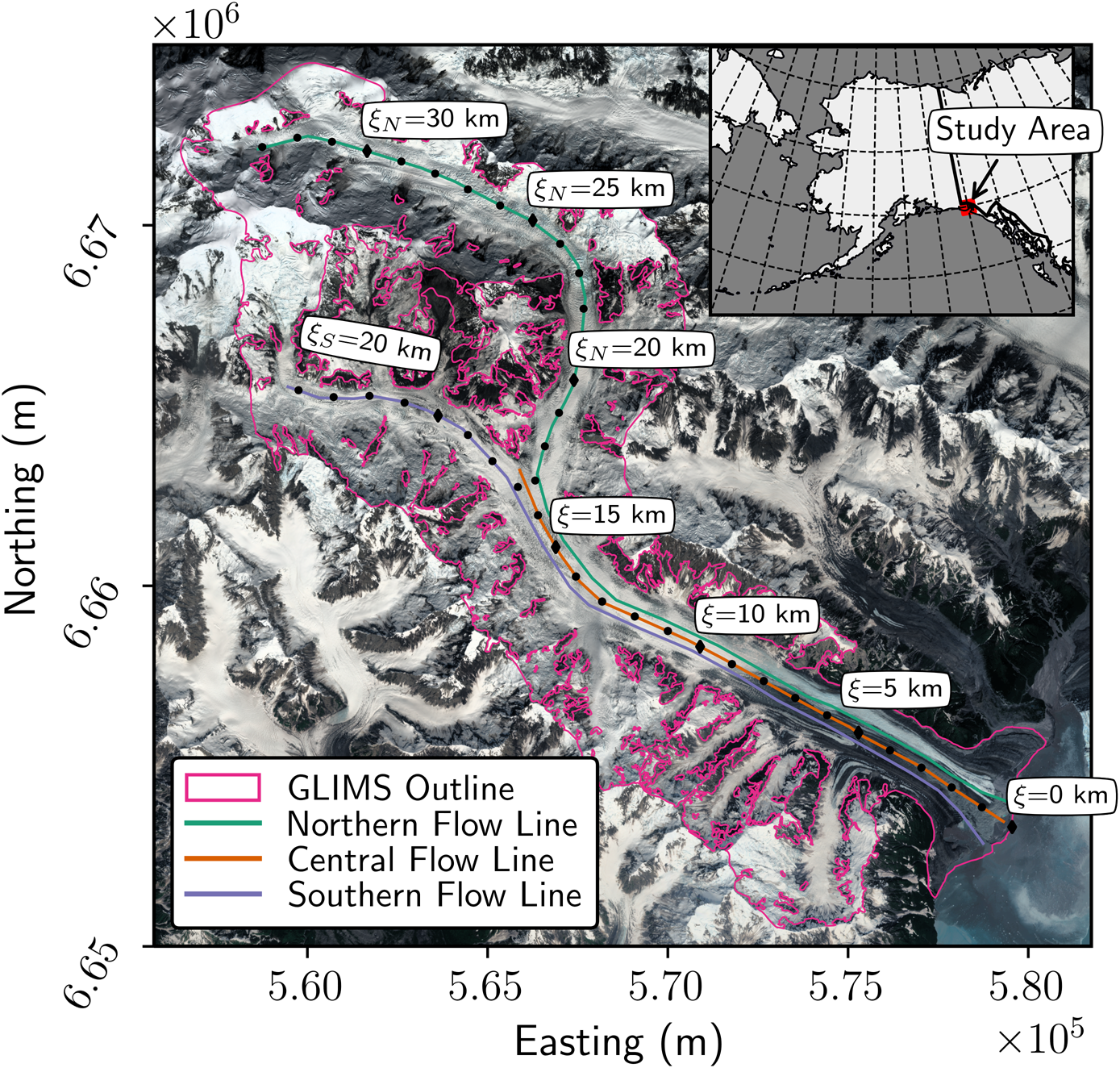
Fig. 1. Sít’ Kusá (60° 02′N, 139° 39′W), St. Elias Mountains, Alaska. Sít’ Kusá is located in Disenchantment Bay, at the toe of Hubbard Glacier to the east. Flowlines shown here are used for velocity and elevation profiles. Black circles mark the distance from the maximum terminus position (ξ) in kilometers, plotted at 1 km intervals. Background imagine is from Sentinel-2 on 31 August 2018 projected on a UTM 7N grid.
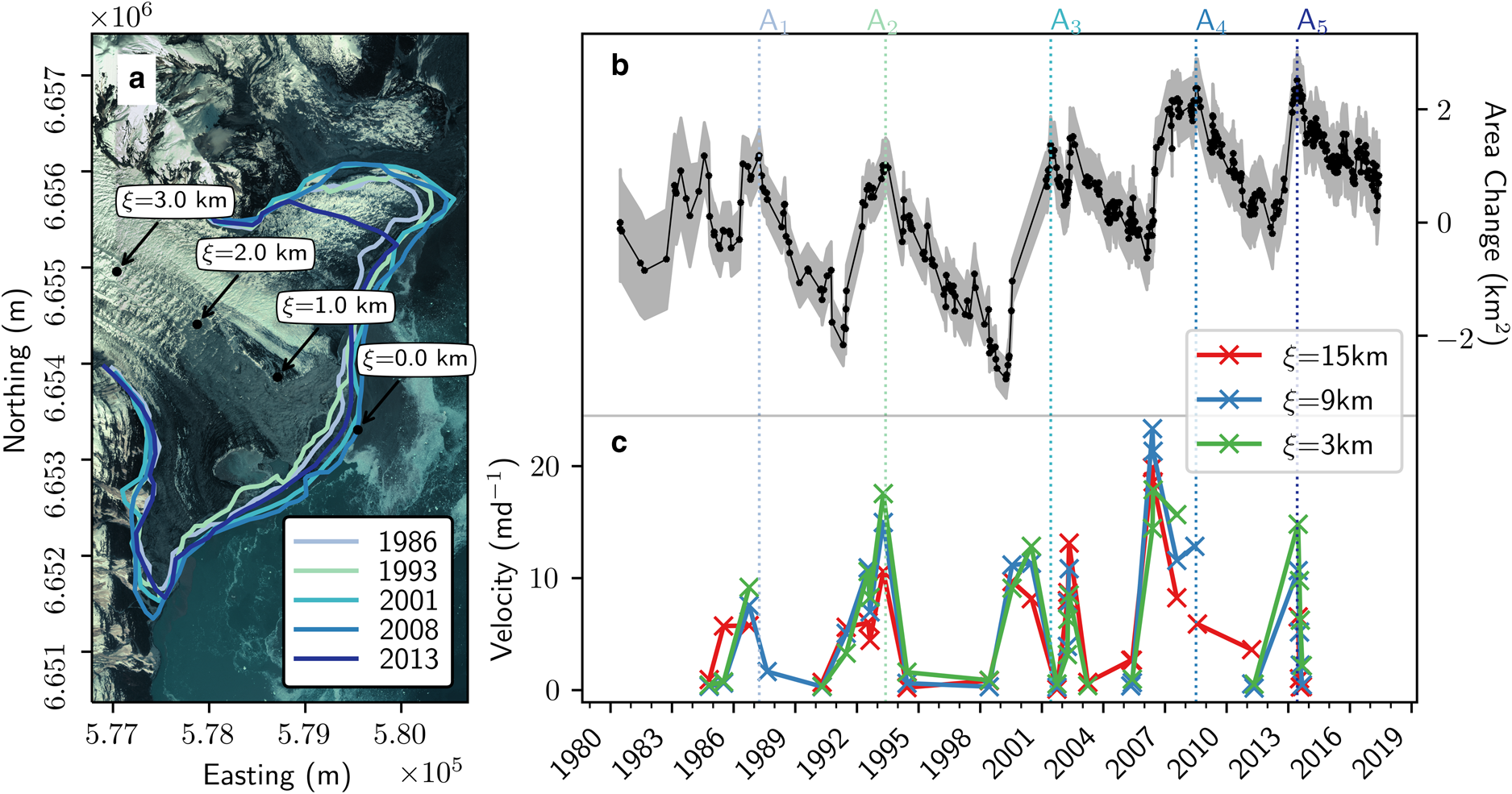
Fig. 2. Area and velocity observations of Sít’ Kusá from 1984 to 2017. (a) Worldview 2 image (Imagery copyright 2016 DigitalGlobe, Inc.) from 10 May 2016 overlain by maximum glacier extent during the five (A1– A5) surge events (Table 2). Black circles mark the distance from the maximum terminus position (ξ) in kilometers, plotted at 1 km intervals. (b) Area change calculated relative to the first observation (4 June 1980). Uncertainty due to mixed pixels is indicated by gray shading. Vertical lines correspond to the date of the maximum terminus area mapped in (a). (c) Surface velocity. Sampling points are denoted by the flow following coordinate system ξ. Points are connected with straight lines only to make the visualization of the velocity variations easier and should not be interpreted as indicative of trends over time.
3. Data and methods
Our analysis used time series of glacier terminus position, surface velocity and surface elevation extracted from optical satellite imagery. We used the Landsat archive to map terminus position from 1980 to 2017 and surface velocity from 1984 to 2013. These observations were paired with sparser digital elevation models (DEM) constructed from a variety of satellite and airborne platforms to quantify surface elevation changes through time. Details on each of these datasets and the methodologies used for their analysis are presented below.
3.1. Terminus delineation
Four Landsat 2 Multi Spectral Scanner (MSS), one Landsat 3 MSS, seven Landsat 4 MSS, one Landsat 4 Thematic Mapper (TM), 163 Landsat 5 TM, 178 Landsat 7 Enhanced Thematic Mapper Plus (ETM+), and 78 Landsat 8 Operational Land Imager (OLI) SWIR-1, NIR, Red false color composites were used to map the terminus position of Sít’ Kusá from 24 June 1980 to 4 June 2017. The orthorectified L1 T scenes were downloaded from the United States Geological Survey's Earth Explorer (https://earthexplorer.usgs.gov). Landsat 7 products containing scan-line errors were used if the scan line gaps were small enough that linear interpolation across the gaps did not distort the terminus shape with respect to the terminus geometry closest in date. Because of Sít’ Kusá's lobate terminus, we manually delineated the terminus position between two fixed tie points located on the lateral margins of the glacier (Fig. 2a) and then closed the terminus polygons to analyze changes in terminus area over time.
For the Landsat images used in our analysis, we assumed the mixed pixel effect (i.e. error in delineations due to pixels that overlap both the glacier terminus and the surrounding terrain/embayment) to be the largest source of uncertainty in terminus delineations. To account for this effect, we assumed that the mapped positions could be in error by up one pixel. We summed the number of pixel intersections along each delineation and multiplied by the pixel resolution of the corresponding image to produce an estimate of uncertainty (Silverio and Jaquet, Reference Silverio and Jaquet2005; Rivera and others, Reference Rivera, Benham, Casassa, Bamber and Dowdeswell2007). Thus, uncertainty in the terminus position is a function of the area of each pixel (3600 m2 for Landsat 2–3 MSS and 900 m2 for Landsat 4–5, 7 and 8; Fig. 2).
3.2. Velocity mapping
Surface flow velocities were mapped from 23 April 1984 to 7 October 2013 using 31 pairs of orthorectified level one Landsat 5 TM, 7 ETM+ and 8 OLI scenes. We used Band 4 (30 m) scenes for Landsat 5 and Band 8 (15 m) scenes for Landsat's 7 and 8 to produce our velocities. We did not use Landsat 7 products containing scan-line errors in our velocity analysis. Extensive cloud cover limited the imagery from which velocities could be extracted, requiring scenes from different path/row combinations to be used in our analysis.
Manual examination of nine scene pairs revealed registration errors that needed to be addressed prior to velocity extraction. To fix these, we matched the poorly coregistered scenes to the ground control scenes used by the USGS for the corresponding path/row (LE07_L1TP_061018_20010719_20160929_01_T1 for 61/18, LE07_L1TP_062018_20010608_20160929_01_T1 for 62/18). To find potential matches, we used normalized cross-correlation on a grid with 400 pixel spacing, matching a 101-pixel kernel within a 401-pixel search window. To avoid erroneous coregistration matches on the moving glacier surfaces, clouds or shadow, we masked glaciers using the Randolph Glacier Inventory 6.0 outlines (RGI Consortium, 2017), and cloud/shadow using the Landsat Quality Assessment (BQA) band provided with each scene. Potential static point matches were filtered based on the strength of the correlation and their fit to a 2-D affine transformation between the images estimated using random sample consensus (Fischler and Bolles, Reference Fischler and Bolles1981), implemented using the scikit-image python package (Van der Walt and others, Reference Van der Walt2014). Using the successfully-matched control points and the TanDEM-X 90 m Global DEM (Rizzoli and others, Reference Rizzoli2017), we then transformed each scene using a first-order rational function model (RFM) transform for L1TP scenes, and a third-order RFM for L1GT/L1GS scenes (e.g. Tao and Hu, Reference Tao and Hu2001). If necessary, the L1GS scenes were then orthorectified based on the methods described in Gao and others (Reference Gao, Masek and Wolfe2009).
After all scene-pairs were adequately coregistered, we used NASA's Ames Stereo Pipeline to perform normalized cross-correlation of repeat satellite imagery following the approach of Shean and others (Reference Shean2016). Normalized cross-correlation was computed in the spatial domain using a Gaussian pyramid approach, where correlation is computed on sub-sampled images and the disparities from sub-sampled images are used to seed finer-resolution disparity maps (Shean and others, Reference Shean2016). As this Gaussian pyramid approach automatically determines the search window size, for each pair we chose the size of the correlation window (i.e. kernel) between 9 and 35 pixels based on the surface conditions and observed flow velocities that produced the most spatially-extensive velocity maps (Table 1). Images with limited surface features and/or low contrast (e.g. snow on surface of glacier or limited illumination) produced the best results with a kernel > 21 pixels. Images with more distinct surface features (e.g. heavy crevassing, debris cover) produced the best results when correlated with a kernel size < 21 pixels. Sensitivity tests of kernel size indicate that variations in kernel size have limited effect on quiescent velocity maps, as any difference in velocity between kernel choices were well within our uncertainty bounds (Fig. S1). For the active phases, larger kernel sizes resulted in slower velocities because more of the glacier's static margins were included in the kernels (Fig. S2). Since spatial smoothing decreases with kernel size, smaller kernel sizes resulted in faster but noisier active-phase velocities (Shean and others, Reference Shean2016). Therefore, we manually selected the smallest kernel size that returned the most accurate velocities (i.e. sufficient spatial averaging to reduce random uncertainties but not enough to bias estimates; Fig. S2; Table 1).
Table 1. Landsat 5 TM (LT05), 7 ETM+ (LE07) and 8 OLI (LC08) scenes and the associated correlation window (i.e. kernel) size used to produce the velocity maps

Scene pair dates (DD/MM/YYYY) and paths (all scenes were from row 18) are also listed. Bias and uncertainty metrics for the magnitude components of the velocity are listed.
We estimated the error of our velocity products by measuring the apparent displacement (in the x and y directions) over bare ground, as determined by the union of a glacier mask (RGI Consortium, 2017), a bare ground mask (Hansen and others, Reference Hansen2013) and the BQA bands for the Landsat scenes. The effects of displacements in the x and y directions on our velocities were then corrected by subtracting the median displacement over the identified bare ground surfaces from the displacement measurements used to compute velocities. We used the median apparent displacement (over bare ground surfaces) as our bias metric and one median absolute deviation (MAD) as our uncertainty metric (Table 1), as they are robust against outliers caused by clouds, shadows and/or rising snow-lines. Nonetheless, the average bias (plus or minus average MAD) prior to displacement corrections was − 0.04 ± 0.60, − 0.06 ± 0.53 and 0.74 ± 0.55 m d−1 in the x, y and magnitude components, respectively (Fig. 3; Table 1). These uncertainties apply to regions with abundant surface features (e.g. chaotic crevasses), including the ablation zone below ξ N = 21 km and the accumulation zone above ξ N = 25 km. Uncertainties are likely larger across the icefall, however, where the ‘standing-wave’ of crevasses causes the correlation algorithm to fail; a phenomena known as ‘surface-locking.’ Across the icefall ‘surface-locking’ results in erroneous speed estimates of ~0 m d−1.

Fig. 3. Median offset (m d−1) over bare ground in the x and y directions prior to displacement corrections for all velocity pairs. Marker symbol denotes the path/row combination of the scene-pair and color denotes the kernel size used for correlation.
After we corrected for median offsets over stable ground, we filtered our velocity products using a signal to noise ratio > 3.5 threshold (Paul and others, Reference Paul2017). Then, velocities (x and y) were filtered for orientation following the approach used by Burgess and others (Reference Burgess, Forster, Larsen and Braun2012). First, we calculated the angle θ between each velocity vector v i,j and the median vector within a neighborhood of width w = 7 pixels, $\tilde {v}^{w}_{i, j}$ :
:

We iteratively removed vectors whose θ was above a threshold of 24, 18 and 12 degrees. The remaining velocity vectors were filtered for magnitude so that $\left \vert v_{i, j} - \tilde {v}^{w}_{i, j}\right \vert$ $> 30\percnt$
 of the mean velocity were removed. Finally, these filtered velocity products (in the x and y directions) were used to create the velocity maps, which were smoothed with a Gaussian kernel of size 7 × 7 pixels to minimize the influence of noise in our interpretation. Velocity measurements were manually extracted from individual pixels along the northern, central and southern flowlines (Fig. 1). We defined a flow following coordinate system ξ, originating (ξ = 0 km) at Sít’ Kusá's maximum terminus position. At the confluence of the two tributaries (ξ = 16 km), we split ξ into two separate coordinates, ξ N and ξ S, following the center flowlines of the north and south tributaries, respectively. In this coordinate system, the heads of the northern and southern tributaries are at ξ N = 33 km and ξ S = 24 km, respectively. We report the average and standard deviation in observed velocities for all three flowlines from the terminus to ξ = 16 km. The reported velocities were restricted to ξ ≤ 16 km so that the averages were unbiased by differences in flowline length and data coverage. On average, velocities were mapped for $86\percnt$
 of the three flowlines over the lower 16 km, with poorer data coverage farther inland at higher elevations. Additionally, as described below, the upper portion of the northern tributary (ξ ≥ 23 km) was not affected by the surges and the inclusion of velocities from this portion of the glacier would bias inter-surge velocity analysis (Figs 6, 8).
3.3. Digital elevation models
Surface elevation changes were documented using four Advanced Spaceborne Thermal Emission and Reflection Radiometer (ASTER), one Satellite Pour l'Observation de la Terre 5 (SPOT5), one Interferometric Synthetic Aperture Radar Alaska (IFSAR-Alaska) and two Digital Globe WorldView-1 DEMs. We used MMASTER to create ASTER DEMs with ~10 m vertical uncertainty and 30 m spatial resolution from April 2001, May 2003, March 2006 and July 2012 stereo imagery (Girod and others, Reference Girod, Nuth, Kääb, McNabb and Galland2017). We used two ArcticDEM strips, derived from WorldView stereo pairs acquired in May and December 2013 (Porter and others, Reference Porter2018). These 2 m-resolution DEMs have an estimated vertical accuracy of ~3 m (Noh and Howat, Reference Noh and Howat2015; Shean and others, Reference Shean2016). We downloaded a 5 m-resolution, 3 m vertical uncertainty IFSAR-Alaska DEM acquired in late summer 2012 from Earth Explorer (https://earthexplorer.usgs.gov/). Finally, we downloaded a September 2007 SPOT5 DEM with a vertical uncertainty of 6 m from the SPIRIT project (https://theia-landsat.cnes.fr; Korona and others, Reference Korona, Berthier, Bernard, Rémy and Thouvenot2009). See Table S2 for full granule names and acquisition dates. All of the DEMs were resampled to 30 m spatial resolution using bilinear interpolation, and coregistered to the 2013 WorldView-1 DEM using the methods of Nuth and Kääb (Reference Nuth and Kääb2011). Average elevation uncertainties along the flowlines were calculated as:

where σΔz is the standard deviation of the elevation change measurements, L is the length over which they were measured, and C is the autocorrelation length (500 m; Howat and others, Reference Howat, Smith, Joughin and Scambos2008).
4. Results
4.1. Surge chronology overview
To explore the general characteristics of the surge events (A1–A5), we used terminus area changes to identify the initiation and termination of surge events (Fig. 2), since the terminus change record is more temporally dense than the velocity and elevation datasets (Table 1; Figs 2, 4). Because surges are defined by changes in flow, not necessarily terminus position, we would ideally use our velocity record to constrain the timing of surge events. For properly tidewater surge-type glaciers in Svalbard terminus retreat does not necessarily mean the end of the active phase, just a increase in frontal ablation (Mansell and others, Reference Mansell, Luckman and Murray2012). However, cloud cover in coastal Alaska prevents the construction of a velocity record with sufficiently dense temporal sampling to confidently identify surge initiation and termination from changes in flow speed.

Fig. 4. Timing of surge initiation and termination for five surge events (A1–A5). The shaded area is the temporal uncertainty of when the changes occurred. The time when the terminus is advancing is denoted by the black brackets.
The rate of terminus position change is calculated as

where L is the glacier length, $\bar {v}_{\rm s}$ is the width-averaged speed at the terminus, and $\bar {v}_{\rm a}$
 is the width averaged rate of frontal ablation (sum of calving and submarine melting). We observe that terminus advance (A1–A5) consistently begins between February and June (Table 2; Fig. 4). Assuming there is no dramatic periodic decrease in $\bar {v}_{\rm a}$
 that initiates the terminus advance every ~5 years, then increases in L (A1–A5) must be driven by an increase in advection toward the terminus ($\bar {v}_{\rm s}$
 ). Thus, we hypothesize that the periodic advance of the terminus through the winter and into spring indicates changes in ice flow toward the terminus. Based on the terminus change time series, paired with velocity and elevation time series when available, we identify five surge events (A1–A5) since 1980 (Table 2; Figs 2, 4). The surge events have an average recurrence interval of ~5 years and an active phase of ~2 years (Table 2). Observations from each surge event are described in detail below.
TABLE 2. Transition between active (A) and quiescent (Q) phases of Sít’ Kusá from 1984 to 2013

The duration (in years) of the surge phase (as inferred by terminus change) and associated terminus change (km2) are listed with corresponding uncertainties. For the active phase, speeds reported are the maximum observed speeds with location of corresponding speeds. For the quiescent phase, we report mean velocities over the trunk ($\xi = 0 - 16\, {\rm km}$ ) of the glacier. Transition between phases are separated by a solid line. Date format is DD/MM/YYYY.
4.2. 1983–1986 Surge event (A 1)
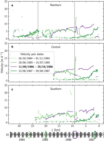
While surge events presumably occurred prior to 1983, we are not confident in the data quality and temporal density prior to 1980. We first observe terminus advance between September 1981 and September 1982 (Table 2, Fig. 2 and 4), with the terminus advancing until late summer 1984. Our first speed observation, in fall 1984, was 0.46 ± 0.37 m d−1 over the trunk of the glacier (Fig. 5). In summer 1985 the mean speed was 2.58 ± 2.05 m d−1, with the largest increase at the confluence ($\xi = 10 - 15\, {\rm km}$ ) of the tributaries (Fig. 5). Terminus advance began again in spring 1986 accompanied by a 11.4-fold increase in mean speed by fall 1986 (Table 2; Figs 4, 5). Terminus advance ceased in spring/summer 1987, ending a 5.6 ± 1.9 year surge event that caused the glacier to advance 2.0 ± 1.0 km2 (Figs 2, 4; Table 2). Velocity maps from August 1987 show quiescent speeds over the whole glacier, except for slightly elevated speeds for ξ < 5 km (Fig. 5).

Fig. 5. 1984–1986 surge speed observations. Speeds extracted along the northern (a), central (b) and southern (c) flowlines with dates for all profiles shown in subplot d. Active phase speeds are denoted in bold on the legend in subplot (b). The vertical grey line at ξ = 9.25 km is the approximate location of the dynamic balance line. The vertical grey line at ξ N = 23 km in (a) is the approximate location of the icefall located on the northern tributary. Date of image pairs plotted on the timeline, with the color of the boxes corresponding to the lines in subplots a–c.
4.3. 1991–1993 Surge event A 2
The glacier appeared to be in quiescence in spring 1990, with a mean speed of 0.61 ± 0.81 m d−1 over its trunk (Figs 6a–c; Table 2). Terminus advance began in May 1991, after retreating 3.4 ± 0.6 km2 since 1986 (Fig. 4; Table 2). Terminus advance was accompanied by a 7.8-fold increase in mean speed in June 1991, as compared to spring 1990 (Figs 6a–c). Elevated surface speeds continued through 1992 and reached a maximum of 26.15 ± 0.82 m d−1 at the terminus in April 1993 (Table 2; Figs 6a–b). Terminus retreat commenced again in 1993 and we observed quiescent speeds through summer 1994 (Table 2; Figs 2, 4, 6a–c). The surge event lasted 2.1 ± 0.2 years, and resulted in a 3.2 ± 0.6 km2 increase in glacier area (Table 2; Fig. 2).

Fig. 6. 1991–1993 surge speed observations. Speeds extracted along the northern (a), central (b) and southern (c) flowlines with dates for all profiles shown in subplot b. Quiescent (active) speeds are colored in green (purple) and become darker in time. Active phase speeds are denoted in bold on the legend in subplot (b). The vertical grey line at ξ = 9.25 km is the approximate location of the dynamic balance line. The vertical grey line at ξ N = 23 km in (a) is the approximate location of the icefall located on the northern tributary. Date of image pairs plotted on the timeline (d), with the color of the boxes corresponding to the lines in subplots a a–c.
4.4. 1999–2002 Surge event (A 3)
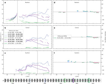
The glacier was in quiescence through 1998, with a mean speed of 0.61 ± 0.61 m d−1 over its trunk in June 1998. The terminus began to advance in April 1999, ending 3.8 ± 0.6 km2 of terminus retreat since the termination of the last surge (Table 2; Figs 4, 2). By summer (14 July–6 August) 1999, the glacier speed increased 15-fold, reaching a peak of 12.52 ± 0.36 m d−1 at ξ = 7.9 km (Fig. 7.) Elevated speeds continued through July 2000, reaching a peak of 17.74 ± 1.03 m d−1 at the terminus (Fig. 7; Table 2). In June 2001, we observed terminus retreat, and by fall of 2001, we recorded quiescent-like speeds of 0.39 ± 0.36 m d−1 over the glacier trunk (Figs 2, 4, 7). This portion of the surge lasted 2.1 ± 0.1 years, and resulted in a 4.1 ± 0.6 km2 increase in glacier area (Figs 2, 4; Table 2).

Fig. 7. 1999–2002 surge speed and elevation change observations. Speeds and elevations extracted along the northern (a, d), central (b, e) and southern (c, f) flowlines with dates for profiles shown in subplots b and e. Quiescent (active) speeds are colored in green (purple) and become darker in time. DEMs are plotted with the color of the velocity map closest to the date range of the differenced DEMs. Date pairs exhibiting active phase speeds are denoted in bold on the legend in subplot (b). The vertical grey line at ξ = 9.25 km (ξ N = 23 km) is the approximate location of the dynamic balance line (northern tributary icefall). Date of speed scene pairs plotted on the timeline (g), with the color of the (solid) boxes corresponding to the lines in subplots a–c. The thinner (dotted) boxes are the time span of DEM pairs.
Terminus retreat continued until early spring (3 February–16 March) 2002 (Figs 2 and 4), resulting in a total retreat of 1.1 ± 0.7 km2 (Table 2). There was a ~14-fold increase in mean speed by early April 2002, as compared to quiescent speeds from summer 2000 (Fig. 7). Active-phase speeds continued through mid-April 2002, reaching 20 times the quiescent speeds, with down-glacier propagation of the surface speed maximum (Fig. 7). Terminus advance ceased during the summer of 2002, for a total advance of 1.2 ± 0.7 km2 since March 2002 (Table 2; Figs 2, 4), and the glacier slowed to quiescent speeds by spring 2003 (Fig. 7).
From April 2001 to 2003, surface elevations decreased by an average of 6.9 ± 1.4 m from $\xi = 0 - 5\, {\rm km}$ across all three flowlines (Figs 7d–e, pink shading). Over the same time period, there was an average increase in elevation of 8.8 ± 0.4 m for all three flowlines above ξ = 5 km (Figs 7d–f, blue shading). Surface elevation increase along the northern flowline was confined to below the icefall at ξ = 23 km (Fig. 7d).
4.5. 2006–2008 Surge event (A 4)
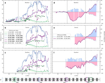
Terminus advance in winter 2006 ended a 5.6 ± 0.1-year quiescent period during which the terminus retreated 2.2 ± 0.8 km2 (Table 2; Figs 2, 4). By May 2006, the glacier had sped up 22.6-fold over its trunk (Fig. 8), reaching a peak of 27.6 ± 1.2 m d−1 at ξ = 10.9 km (Table 2; Figs 8a–c). Active-phase speeds continued through summer 2007, with a surface speed maximum (of 18.49 ± 0.32 m d−1) at ξ = 2.7 km (Fig. 8). By summer 2008, velocities decreased ~65% relative to summer 2007, and the terminus began to retreat (Table 2; Figs 2, 4, 8a–c). The surge event lasted 2.4 ± 0.2 years and was associated with a 3.0 ± 0.8 km2 increase in area (Fig. 2; Table 2).

Fig. 8. 2006–2008 surge speed and elevation change observations. Speeds and elevations extracted along the northern (a, d), central (b, e) and southern (c, f) flowlines with dates for profiles shown in subplots b and e. Quiescent (active) speeds are colored in green (purple) and become darker in time. Differenced DEMs (d–f) are plotted with the color of the velocity map closet to the date range of the differenced DEMs, with thickening shaded in blue and thinning in red. Date pairs exhibiting active phase speeds are denoted in bold on the legend in subplot (b). The vertical grey line at ξ = 9.25 km (ξ N = 23 km) is the approximate location of the dynamic balance line (northern tributary icefall). Date of speed scene pairs plotted on the timeline (g), with the color of the (solid) boxes corresponding to the lines in subplots a–c. The thinner (dotted) boxes are the time span of DEM pairs.
From 20 May 2003 to 3 March 2006, a time period including both the quiescent phase and surge initiation, the glacier surface elevation increased by an average of 28.7 ± 1.1 m above ξ = 9.3 km (Figs 8d–f, blue shading). For all three flowlines, the surface elevation decreased over $\xi = 0 - 10\, {\rm km}$ by an average of 28.9 ± 1.5 m (Figs 8d–e, pink shading). The along-flow patterns of surface elevation change were reversed from March 2006 to September 2007, during the active phase of the surge. Surface elevations increased over $\xi = 0 - 7\, {\rm km}$
 by an average of 54.5 ± 3.8 m, with a maximum increase of 141 ± 12.0 m at the terminus (Figs 8d–f, dark blue line). Above the dynamic balance line (ξ = 9.25 km), the surface lowered by 56.9 ± 2.0 m on average, with a maximum thinning of 123.6 ± 12.0 m at ξ N = 18.1 km (Fig. 8d). Over both time periods (May 2003 to March 2006 and March 2006 to September 2007), little change occurred above ξ N = 23 km, the approximate location of the icefall (Fig. 8d).
4.6. 2011–2013 Surge event (A5)
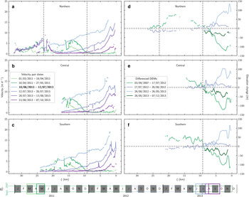
The glacier was in quiescence for 3.7 ± 0.2 years, through spring of 2011, during which the glacier retreated 2.6 ± 0.8 km2 (Table 2; Figs 2, 9a–c). While quiescent speeds were uniform below ξ < 10 km, we see an increase in speed at the confluence of the two tributaries ($\xi = 10 - 15\, {\rm km}$ ) through the spring of 2011 (Figs 9a–c). Terminus advance began in spring 2012.

Fig. 9. 2011–2013 surge speed and elevation change observations. Speeds and elevations extracted along the northern (a, d), central (b, e) and southern (c, f) flowlines with dates for profiles shown in subplot b and e. Quiescent (active) speeds are colored in green (purple) and become darker in time. Differenced DEMs (d–f) are plotted with the color of the velocity map closet to the date range of the differenced DEMs, with thickening shaded in blue and thinning in red. Date pairs exhibiting active phase speeds are denoted in bold on the legend in subplot (b). The vertical grey line at ξ = 9.25 km (ξ N = 23 km) is the approximate location of the dynamic balance line (northern tributary icefall). Date of speed scene pairs plotted on the timeline (g), with the color of the (solid) boxes corresponding to the lines in subplots a-c. The thinner (dotted) boxes are the time span of DEM pairs.
We first observed active-phase speeds in June 2013, a ninefold increase from early-spring 2011, with a surface speed maximum of 19.04 ± 0.27 m d−1 at ξ = 2 km (Figs 9a–c). Speeds decelerated, propagating downglacier, through the summer of 2013 (Figs 9a–c). Our final observation from fall 2013 shows quiescent speeds over the entire glacier, except ξ < 5 km where mean speeds were 1.68 ± 0.24 m d−1. Terminus retreat began in early summer 2013, signaling the end of a 1.2 ± 0.2 year surge event, where the glacier advanced 2.6 ± 0.8 km2.
Elevation observations from September 2007 to July 2012 (spanning the quiescent period) show a mean surface lowering of 59.93 ± 0.4 m from $\xi = 0 - 9\, {\rm km}$ and an average thickening of 31.6 ± 1.1 m above ξ = 9 km (Figs 9d–f). From July 2012 to late August 2012, the glacier surface lowered by 3.0 ± 0.4 m above ξ = 10 km and thickened by 32.9 ± 0.7 m below ξ = 10 km on average (Figs 9d–f). The May 2013 DEM only covers the lowest 9 km of the glacier, but shows an average thickening of 45.9 ± 4.3 m as compared to August 2012 (Figs 9d–f). From May to December 2013, surface elevation decreased by an average of 26.6 ± 1.2 m over ξ = 0 − 9 km (Figs 9d–f).
4.7. Inter-surge comparison
Sít’ Kusá surged five times between 1980 and 2017, making it one of the most active surge-type glacier currently known in the world (Table 2; Fig. 2; Sevestre and Benn, Reference Sevestre and Benn2015). We find that, on average, surge events have an active phase of ~2 years and a recurrence interval of ~5 years (Table 2; Fig. 2). We observe as much as 20-fold increases in speed (e.g. A 2, A 4) during the active-phase. Preceding surge-initiation, we observe increased surface speeds at the confluence ($\xi = 10 - 15\, {\rm km}$ ) of the two tributaries (e.g. Figs 5, 6, 8, 9). Terminus advance consistently begins between February and May (Table 2; Fig. 4). During the active-phase of surge events, we observe surface-speed maximums propagate down-glacier (Figs 5–9). Elevation change observations suggest the boundary between the reservoir zone and the receiving zone (i.e. dynamic balance line) is at ξ ≈ 9 km (Figs 8 and 9). For the northern tributary, the inland extent of the reservoir zone coincides with the base of the icefall located at ξ N = 23 km (Figs 7, 8). Surface elevation profiles from the 2006–2008 surge event (A4) suggest the reservoir zone extends over the entire southern tributary above ξ = 9 km (Fig. 8f). Based on the extent of surface elevation gain during the 2006–2008 (A 4) and 2011–2013 (A 5) surge events, we infer that the receiving zone extends from ξ ≈ 9 km to the terminus.
5. Discussion
5.1. Probable surge mechanism
Our sparse sampling of velocities is dictated by extensive cloud-cover in southeast Alaska. Therefore, we note that our maximum speeds only represent what we are able to observe, and do not coincide with the actual maximum speed of the glacier during each surge event. Nonetheless, elevated speeds over the entire glacier (excluding the area above the icefall) during the active phase support our use of terminus position change as an indicator of surge advance, since enhanced flow toward the terminus will result in terminus advance in the absence of an equivalent change in calving and/or submarine melting (Eqn (3)). While McNabb and others (Reference McNabb, Hock and Huss2015) document variations in frontal ablation for Sít’ Kusá, their estimates are based solely on surface velocities and changes in terminus position. Because McNabb and others (Reference McNabb, Hock and Huss2015) did not have coincident elevation change observations, we cannot partition their rates of frontal ablation between oceanic forcing and glacier dynamics. We observe terminus advance consistently beginning between February and May (Table 2; Fig. 4), suggesting surge events initiate in late winter at Sít’ Kusá. Late winter surge initiation has been observed for a number of glaciers, including Variegated Glacier (Kamb and others, Reference Kamb1985; Eisen and others, Reference Eisen2005), Medvezhiy Glacier (Dolgoushin and Osipova, Reference Dolgoushin and Osipova1975), West Fork Glacier (Harrison and others, Reference Harrison, Echelmeyer, Chacho, Raymond and Benedict1994), Bering Glacier (Roush and others, Reference Roush, Lingle, Guritz, Fatland and Voronina2003) and Sortebræ (Pritchard and others, Reference Pritchard, Murray, Luckman, Strozzi and Barr2005), and is commonly attributed to pressurization of an inefficient subglacial hydrologic network and enhanced basal sliding (Kamb, Reference Kamb1987). For hydrologically-regulated surges, the surge front propagates down-glacier (Meier and Post, Reference Meier and Post1969; Dolgoushin and Osipova, Reference Dolgoushin and Osipova1975), which we also observe at Sít’ Kusá (Figs 5–9). Thus, we interpret the apparent winter initiation in conjunction with down-glacier propagation to suggest the hydrologic switch as the mechanism responsible for Sít’ Kusá's surges. Both observational (e.g. Clarke and others, Reference Clarke, Collins and Thompson1984; Truffer and others, Reference Truffer, Harrison and Echelmeyer2000; Woodward and others, Reference Woodward, Murray, Clark and Stuart2003) and theoretical studies (e.g. Clarke, Reference Clarke1987b; Minchew and Meyer, Reference Minchew and Meyer2020) suggest the deformation of till to be a critical component in the initiation and propagation of surge events, while till has also been proposed as the mechanism controlling the fast flow of icecaps in Iceland (e.g. Boulton and Hindmarsh, Reference Boulton and Hindmarsh1987; Kjær and others, Reference Kjær2006; Minchew and others, Reference Minchew2016) and ice streams in Antarctica (e.g. Blankenship and others, Reference Blankenship, Bentley, Rooney and Alley1987; Tulaczyk and others, Reference Tulaczyk, Kamb and Engelhardt2000). Given the high sediment production rates at Sít’ Kusá (Goff and others, Reference Goff, Lawson, Willems, Davis and Gulick2012), it likely overlies a soft bed of deformable sediments, which could play an important role in surge initiation and propagation. We currently lack sufficient observations to make conclusions about the till, highlighting the importance of future work here to understand the subglacial environment.
5.2. Controls on surge recurrence intervals
While the kinematics of Sít’ Kusá's surge cycle are similar to its land-based Alaskan counterparts, its recurrence interval is exceptionally short. The typical surge recurrence interval in Alaska for temperate, hydrologically-regulated surge events is about 15 years (Sevestre and Benn, Reference Sevestre and Benn2015). Variegated Glacier's surge recurrence interval is 13–18 years (Eisen and others, Reference Eisen, Harrison and Raymond2001), for Lowell Glacier between 11 and 18 years (Bevington and Copland, Reference Bevington and Copland2014), and 9–12 years for Donjek Glacier (Kochtitzky and others, Reference Kochtitzky2019). Environmental conditions (thermal regime and precipitation) have been suggested as an explanation for regional differences in the length of the surge cycles between Svalbard (50–100 year quiescent period and 3–10 year active phases) and Alaska/Yukon (10–15 year quiescent period and 1–2 year active phases; Dowdeswell and others, Reference Dowdeswell, Hamilton and Hagen1991; Murray and others, Reference Murray, Strozzi, Luckman, Jiskoot and Christakos2003). However, environmental and geometric factors that influence reservoir evacuation also likely influence surge recurrence intervals. For example, the 1995 surge of Variegated terminated early with respect to previous surges (Eisen and others, Reference Eisen2005) and the next surge occurred only 9 years later in 2003/2004, a recurrence interval much shorter than the previously observed 13–18 years (Harrison and others, Reference Harrison2008). This anomalously short surge interval has been attributed to the early termination of the 1995 surge, which resulted in only partial evacuation of the reservoir zone and reduced the mass accumulation required to reach the critical stress threshold for surge initiation (Eisen and others, Reference Eisen2005; Harrison and others, Reference Harrison2008). While environmental conditions are clearly important, it remains difficult to isolate their impact on the surge cycle.
Given Sít’ Kusá's location in southeast Alaska, an area characterized by high accumulation rates (Marcus and Ragle, Reference Marcus and Ragle1970), it is important to understand the influence of climate and mass balance on Sít’ Kusá's surge kinematics. While glacier surges are known to be caused by internal dynamics, climate is an important control on the distribution of surge-type glaciers (Sevestre and Benn, Reference Sevestre and Benn2015), surge recurrence intervals (Eisen and others, Reference Eisen, Harrison and Raymond2001; Striberger and others, Reference Striberger2011), the vigor of the active phase (Frappé and Clarke, Reference Frappé and Clarke2007) and regional changes in the number of surge-type glaciers (Dowdeswell and others, Reference Dowdeswell, Hamilton and Hagen1991; Copland and others, Reference Copland2011). The link between climate and surge recurrence is supported by geologic evidence of glaciers that were formerly surge-type under more suitable climatic conditions (Hoinkes, Reference Hoinkes1969) and the correlation of surge recurrence intervals with centennial to millennial climatic variability (Striberger and others, Reference Striberger2011). Accumulation data, from one ablation stake, for Variegated Glacier shows a threshold of 43.5 ± 1.2 m must be reached for surge initiation to occur, a quantity that remains constant despite variations in the length of the recurrence interval (Eisen and others, Reference Eisen, Harrison and Raymond2001). Sít’ Kusá is located ~ 20 km away from Variegated Glacier, just across Disenchantment Bay. While Sít’ Kusá is a much larger glacier (177.0 versus 36.3 km2; RGI Consortium, 2017) and extends to higher elevations (Fig. 10) where we know little about the mass-balance profile, it experiences similar regional climatic conditions to Variegated. Therefore, if mass balance were the sole factor dictating a glacier's ability to reach the critical basal shear stress needed for surge-initiation, we would expect Sít’ Kusá and Variegated to surge at similar frequencies. The fact that they do not demonstrate that external forcings alone are insufficient to cause a glacier to surge or explain the heterogeneity in surge kinematics within a geographic region (i.e. Sít’ Kusá versus Variegated).

Fig. 10. Hypsometry for Sít’ Kusá and Variegated Glacier. Curves show the normalized distribution of ice area with elevation, such that the area under each curve is equal. Elevation data comes from IFSAR-Alaska DEM from August 2012. Long dashed lines indicate the mean elevations and short dashed lines indicate plus or minus one standard deviation.
5.3. Possible explanations for Sít’ Kusá's exceptional recurrence interval
Eisen and others (Reference Eisen2005) hypothesize that surge events initiate when the reservoir zone fills sufficiently and reaches a critical basal shear stress. This assumes the driving stress equates to the basal shear (τb) stress:

where F is a shape factor, ρ is the ice density, g is the acceleration due to gravity, H is ice-thickness and α is the surface slope. This assumption has been shown to be invalid during surge-initiation (Schoof, Reference Schoof2005), when the driving stress and basal shear stress do not equate, due to rapid changes in effective pressure. Nonetheless, we use this crude approximation for a conceptual discussion of the quiescent period leading to surge-initiation. Changes in ice-thickness (H) with time are dictated by:

both the flux divergence ($\nabla \cdot Q$ ) and the mass balance ($\dot b$
 ). Assuming the mass balance between Sít’ Kusá and Variegated are similar enough to be insufficient to explain the dramatically different surge-recurrence intervals, we suggest that geometric factors that control the flux-divergence ($\nabla \cdot Q$
 ) play a role in Sít’ Kusá's exceptionally short recurrence interval.
Velocity and surface elevation observations, from the 2006–2008 surge in particular, show surge speed and mass redistribution confined to $\xi _N = 0 - 22\, {\rm km}$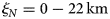 by the icefall at ξ N = 23 km (Figs 7–9). The observed disconnect in kinematics above and below the icefall is in line with the observations of large flow speed changes and mass redistribution below icefalls at a number of glaciers in Alaska (e.g. McNabb and others, Reference McNabb2012; Armstrong and others, Reference Armstrong, Anderson and Fahnestock2017; Durkin and others, Reference Durkin, Bartholomaus, Willis and Pard2017; Enderlin and others, Reference Enderlin, O'Neel, Bartholomaus and Joughin2018) and previous observations of glacier surges confined by an icefall (e.g. Echelmeyer and others, Reference Echelmeyer, Butterfield and Cuillard1987; Pritchard and others, Reference Pritchard, Murray, Strozzi, Barr and Luckman2003). This disconnect in kinematics likely inhibits draw down of ice volume from the accumulation zone during a surge event, as supported by the minimal observed elevation changes above ξ N = 23 km during the 2006–2008 surge (Fig. 8). Although our velocity observations are temporally sparse, the data suggest that advection from the northern tributary's accumulation zone is either relatively steady or slightly elevated after surges (Figs 7–9), enabling rapid accumulation of ice in the reservoir zone between surge events. Due to the likelihood of surface locking across the icefall, which may bias our velocity time series in this location, we cannot confidently interpret temporal variations (or lack thereof) in speed across the icefall ($\xi _N\approx 22 - 24\, {\rm km}$
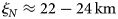 ). However, Sít’ Kusá's extensive crevassing enables successful offset tracking in the isolated accumulation zone above the icefall (Figs 5–9). It is unlikely that surge events initiate at the icefall, but the icefall does appear, in part, responsible for the rapid filling of the reservoir zone leading to surge initiation. The elevated surface speeds on the main trunk of the glacier (Figs 5, 6, 8, 9), which propagate down-glacier (Figs 8, 9), suggest surge events initiate somewhere along the confluence of the two tributaries ($\xi = 10 - 15\, {\rm km}$
 ).
).
Flowers and others (Reference Flowers, Roux, Pimentel and Schoof2011) note a similar kinematic disconnect during surge events above and below a pronounced bedrock ridge of a small surge-type glacier in Yukon, Canada. While the kinematic disconnect does not alter the recurrence interval for the glacier in that study, prognostic numerical modeling simulations under a warming climate suggest the bedrock ridge contributes to the glacier's ability to form a reservoir zone even when climatic conditions are sufficiently negative to inhibit surging (Flowers and others, Reference Flowers, Roux, Pimentel and Schoof2011). Therefore, glacier geometry, especially bedrock topography, not only affects surge characteristics, it may also influence (locally) if and how a glacier will surge under a warming climate.
In summary, our analysis of several surge cycles of Sít’ Kusá is consistent with a model of surging where surge propagation is facilitated by an inefficient subglacial drainage system (Kamb, Reference Kamb1987; Eisen and others, Reference Eisen2005; Harrison and others, Reference Harrison2008). We do not have sufficient data to fully assess the role of glacier geometry on Sít’ Kusá's surge characteristics, but we interpret the muted surface velocity and surface elevation changes inland of the northern tributary's icefall (at ξ N = 23 km) as an indicator that the underlying topography strongly influences the characteristics of the glacier's surges. Although it is well known that an interplay between climate and geometry influence surge behavior, we recommend future investigation of Sít’ Kusá's exceptionally short recurrence interval with more detailed observational data to gain unique insights into controls on glacier surging.
6. Conclusion
From our analysis of optical satellite archives, we document five surge events of Sít’ Kusá between 1980 and 2013. Surge events lasted ~2 years on average with an average ~5-year recurrence interval between surges, representing the shortest known regular recurrence interval in the world (Table 2). We observe terminus advance to consistently begin between February and May, corresponding to hydrologic winter, for the 1991–1993, 1999–2002, 2006–2008 and 2011–2013 (A2–A5) surge events (Fig. 4). Velocity observations from the A1–A5 surge events (Figs 5–9) show down-glacier propagation of surface speed maximums over the course of each surge event. Surface elevation observations from the 2006–2008 (A4) and 2011–2013 (A5) surge events reveal the dynamic balance line to be 9 km from the terminus with the reservoir zone extending over the entire southern tributary while mass redistributions are confined below the icefall along the northern flowline at ξ N = 23 km (Figs 8–9). Based on the winter initiation, down-glacier propagation, and geographic location, we believe Sít’ Kusá's surge events are hydrologically regulated. The kinematic discontent above and below the icefall (ξ N = 23 km) may explain the rapid recurrence interval of Sít’ Kusá. In order to understand what drives the recurrence interval, and therefore surge initiation, more detailed investigation to the fluxes coming from the isolated reservoir zone is needed. Additionally, characterization of basal properties, glacier dynamics, and surface accumulation and melt during quiescent and active phases will facilitate an improved understanding of hydrologic controls on surging at Sít’ Kusá. Given similarities between Sít’ Kusá's surge characteristics and other Alaskan surge-type glaciers, we recommend that future studies of glacier surging leverage Sít’ Kusá's exceptionally short recurrence interval to advance not only the understanding of surge initiation and propagation at this particular glacier, but all glaciers that undergo dynamic instabilities attributed to rapid changes in subglacial hydrology.
Supplementary material
The supplementary material for this article can be found at https://doi.org/10.1017/jog.2021.29
Data availability
All Landsat imagery used in our analysis is available from https://earthexplorer.usgs.gov/. The terminus position timeseries (Fig. 2), filtered velocity products and DEMs (Figs 5–9) are archived online at https://zenodo.org/record/4382724.
Acknowledgements
A.N. was supported by the Maine Space Grant Consortium and the Golden Fund. A.N. acknowledges support provided by WestGrid (www.westgrid.ca) and Compute Canada Calcul Canada (www.computecanada.ca). W.K. was supported by the National Science Foundation Graduate Research Fellowship under grant No. DGE-1144205. R.M. acknowledges support from the European Space Agency through Glaciers_CCI and CCI+ (4000109873/14/I-NB, 4000127593/19/I-NS), and by the European Research Council under the European Union's Seventh Framework Programme (FP/2007-2013) / ERC grant agreement No. 320816. WorldView imagery and DEMs were provided by the Polar Geospatial Center under NSF-OPP awards 1043681, 1559691 and 1542736. A.N. and W.K. thank the Explorers Club and Geologic Society of America for providing funding for a 2018 field season. K.K. was supported by NSF-AGS award 1502783. We thank Hester Jiskoot for her helpful conversations about surging that informed this manuscript through the RemoteEx partnership exchange program, funded by the Norwegian Agency for International Cooperation and Quality Enhancement in Higher Education and in her capacity as Chief Editor. We also thank Scientific Editor Shad O'Neel, William Armstrong and two anonymous reviewers for constructive feedback which helped improve the quality of the manuscript. Finally, we would like to acknowledge the Yakutat Tlingit Tribe on whose land Sít’ Kusá lies.
Author contributions
A.N. delineated the terminus positions, generated the velocity maps, produced figures and wrote a majority of the manuscript. W.K. provided guidance in data generation and methodology, aided in the interpretation of results and helped with manuscript revisions. E.E. played a direct supervisory role at all stages of the project providing guidance on methodology, interpretation of results and manuscript revisions. R.M. processed DEMs, geometrically corrected images and helped with the interpretations of results and revisions of the manuscript. K.K. helped with manuscript revision and provided a supervisory role.


 Open access