


1. Introduction
Brazil has increased agricultural production in recent decades and has engaged in stronger participation in the global market. In spite of increased production, rural populations continue to deal with high-income inequality. Commercial agricultural production remains concentrated in large farms, with approximately 85% of gross agricultural income being generated by 11.4% of Brazilian farms (Alves et al., Reference Alves, Souza and Rocha2013). Barros et al. (Reference Barros, de Carvalho, Franco and Mendonça2006) and Helfand et al. (Reference Helfand, Rocha and Vinhais2009) found evidence of great inequality in rural areas of Brazil using the Gini index. Although income inequality has decreased over time, much remains to be done in order to achieve lower levels of income inequality.
Several factors could contribute to a more equal income distribution in rural areas, including access to rural extension and financial markets. The Brazilian government has implemented several public policies aimed at decreasing income inequality. These policies were based on programs such as income transfer, pension, and credit, but they have shown only a modest contribution to the decrease of rural income inequality (Barros et al., Reference Barros, de Carvalho, Franco and Mendonça2006; Soares, Reference Soares, Ribas and Osório2010; Batista and Neder, Reference Batista and Neder2014).
In 1965, Brazil created the National Rural Credit System (SNCR) to enhance agricultural production and improve the living standards of rural households. The National Agricultural Policy, created in 1991, also contributed to income generation in rural areas of Brazil. Although these instruments sought to improve rural income distribution, they have obtained questionable outcomes. Vega (Reference Vega and Dale1987), Bacha, Danelon and Belson (Reference Bacha, Danelon and Bel Filho2005), and Araújo (Reference Araújo2011) found that large farmers are obtaining greater benefit from access to credit than small farmers.
To overcome inequality in the distribution of benefits, the Brazilian government created the Program for the Strengthening of Family Farming (PRONAF) in 1995. This program seeks to stimulate income generation for small farms that face low productivity and are unable to obtain inputs to modernize their farm and increase productivity (Guanziroli, Reference Guanziroli2007; Santana et al., Reference Santana, Buainain, Silva, Garcia and Loyola2014). However, Corrêa and Silva (Reference Corrêa and Silva2004) and Guanziroli (Reference Guanziroli2007) also suggest that this program is not achieving its initial goal of decreasing inequality.
We have observed a consensus in the literature indicating that, although Brazil has improved rural household access to financial markets (also represented in access to credit), income inequality in these areas remains high and the policies established to combat inequality have been benefiting larger farms. The literature lacks research identifying the additional factors contributing to reductions in rural inequality, such as rural extension, which boost the effect of credit on household income. The literature also lacks analyses that break down the effect of credit on income by income quantiles (e.g., access to credit might have a stronger effect on income in households with a higher income compared to those with a lower income). In this paper, we address these two major limitations by estimating the effect of credit on household income in rural areas of Brazil.
To determine the influence of credit on household income, we use an income decomposition proposed by Firpo et al. (Reference Firpo2007) and the household survey of 2014 from the IBGE (National Household Sample Survey—PNAD). This approach consists of two steps. First, we estimate income regressions for different unconditional quantiles of the income distribution. Second, the income differential is then decomposed into return and composition effects to identify the main factors that explain the income gap across all analyzed quantiles. In addition to this decomposition, we also identify additional factors that are important to the effectiveness of this policy, such as farmer schooling and access to rural extension. Notably, this analysis would be very helpful for guiding the design of new public policies seeking to integrate different agricultural policies such as PRONAF and rural extension.
Our results suggest that credit has led to higher household income inequality in rural areas of Brazil. We determined that households within higher income quantiles observed greater benefits from accessing credit compared to those in lower quantiles. Households that have also had access to rural extension observe more benefits from accessing credit contracts. This combined effect of credit extension is higher among households in the top income quantiles. These results indicate that the coordination of public policies on access to credit and rural extension simultaneously would result in higher benefits to households in rural areas.
2. Background
In Brazil, public policies on rural credit took shape in 1965 with the National Rural Credit System (SNRC). The SNRC was in charge of operating the rural credit policy, which was considered one of the main pillars to agricultural modernization (Santana et al., Reference Santana, Buainain, Silva, Garcia and Loyola2014). Overall, these policies aimed to create structural changes to national agriculture. Public policies in rural credit have undergone three distinct phases between 1969 and 2012 (Buainain et al., Reference Buainain, Carlos, Santana, Silva, Garcia and Loyola2014). In the first phase, between 1969 and 1979, the total volume of credit granted to producers and cooperatives grew substantially in real terms, from R$ 32 billion to R$ 161 billionFootnote 1. In the second phase, between 1979 and 1996 (during the Brazilian government debt crisis), fiscal reforms and stabilization plans led to a decrease in the supply of credit, registering the lowest value of R$ 23 billion in 1996. Total credit supply increased gradually in the third phase, reaching R$ 115 billion in 2012.
Rural credit has been used as one of the main instruments to incentivize agricultural production (Alves, Reference Alves1993; Bacha, Danelon and Belson, Reference Bacha, Danelon and Bel Filho2005; Araújo, Reference Araújo2011; Garcias and Kassouf, Reference Garcias and Kassouf2016). However, it has generated larger benefits to larger farms mostly because these farms have also received access to other services and better production inputs. In 1995, the PRONAF, also connected to the SNRC, was created to provide credit to small farms.
Family-owned farms are predominantly small farms that play an important role in the Brazilian economy. They represent more than 70% of rural establishments and generate 38% of the total value produced in agriculture (IBGE, 2017). In order to have access to credit from PRONAF, family-owned farms must fall within certain eligibility categories highlighted in the Declaration of Aptitude (DAP) to PRONAF Eligibility. The DAP states the maximum and minimum annual income from agricultural activities, property size, land tenure type, and residency in/near to rural property (BNDES, 2015). The supply of credit using this instrument has continuously increased since its creation. In its first year, PRONAF provided 307,000 contracts and R$ 543 million in total loans, while 1.8 million contracts were signed using this instrument—totaling R$ 15.3 billion—in 2012. Notably, the number of contracts nearly doubled in the 2015/2016 crop season (Araújo, Reference Araújo2011; Grisa et al., Reference Grisa, Wesz Junior and Buchweitz2014; Bianchini, Reference Bianchini2015).
2.1. Income inequality and rural credit
Several studies have investigated the determinants of income and income inequality in rural areas of Brazil while considering aspects related to rural credit access. Ferraz et al. (Reference Ferraz, Pase, Brandao, Ferraz and Balcewicz2008) used 2007 data from the Ministry of Finance and the direct comparison method. They concluded that both microcredit policies and lower interest rates correspond to an effective instrument for incentivize investments in productive activities and mitigate poverty. Notably, these instruments are effective when applied to low-income farmers. Batista and Neder (Reference Batista and Neder2014) also investigated the effects of PRONAF on rural poverty in Brazil between 2001 and 2009. They assumed that this instrument does not affect rural poverty directly but does affect the variation of income and/or the variation in income inequality. They used the PNAD database and data from the Central Bank of Brazil in a dynamic panel approach. They determined that PRONAF spending tends to indirectly reduce poverty by raising average income and reducing income concentration.
Souza et al. (Reference Souza, Ponciano, Ney and Fornazier2013) analyzed the inequality in PRONAF’s credit distribution across the country using a descriptive approach and data from the Central Bank of Brazil. They found that, in the initial phase of the program, there was a strong increase in the number of contracts, which continued until 2006 and was followed by an increase in the average size of contracts. They also observed an increase in the participation of states with more capitalized agriculture. An analysis of the evolution of the program has shown that the distribution of credit in Brazil is unequal. However, Kageyama (Reference Kageyama2003) used field survey data from eight Brazilian states in 2001 and applied a multiple regression analysis to compare PRONAF borrowers and non-borrowers, finding no evidence of a positive effect of access to credit on household income, poverty reduction, or educational advancement among family-owned farms. Feijó (Reference Feijó2001) also found a similar result, which indicated that farms with access to the program exhibited lower productivity growth compared to the control group.
Previous studies also investigated the effect of credit on income in other countries. Wan and Zhou (Reference Wan and Zhou2005) investigated the determinants of income inequality in rural China using a regression-based decomposition framework. They concluded that geographic location has been the dominant factor explaining inequality. They found that the most significant determinant of income inequality is the input capital. Mahjabeen (Reference Mahjabeen2008) examined the welfare and distributional implications of microfinance institutions in Bangladesh using a general equilibrium framework and found that microcredit increased the income and consumption levels of households, reduced income inequality, and enhanced welfare. Luan and Bauer (Reference Luan and Bauer2016) examined the heterogeneity of rural credit effects in Vietnam using a data set of 1,338 households collected from the Vietnam Access Resources Household Survey in 2012. They used propensity score matching to evaluate this issue and found that access to credit had a positive effect on household income among households with higher income and access to large amounts of credit.
3. Empirical strategy
To estimate how access to credit affects (not in a causal way) household income, we use the National Household Sample Survey (PNAD) for 2014 from the IBGEFootnote 2. This survey also provides a supplementary questionnaire that includes questions related to the access to and sources of credit for rural production. This survey categorizes rural credit into (i) PRONAF and (ii) other sources (i.e., other public programs and/or banking loans for rural usage). These questions were used to build dummy variables as a proxy for whether or not the farmer had access to rural credit.
Our data set is a subsample of the PNAD, which includes rural households only. Similar to Ely et al. (Reference Ely, Parfitt, Carraro and Ribeiro2017), our sample considers rural producers that are (i) economically active; (ii) employers or self-employed workers (these being the individuals interviewed in the questionnaire); and (iii) mainly occupied by agricultural activity. Our sample also included a small portion of rural property managers that live in urban areas (IBGE, 2017). After excluding missing values and outliers, the final sample consisted of 15,402 individuals.
Our dependent variable is monthly household income in R$ (Reais—Brazilian currency), which is a proxy for farmer income. To control for other factors that also influence household income level, we also included:
a) gender: a dummy variable equals 1 if the individual is male;
b) race: a dummy variable equals 1 if the individual is black;
c) schooling: several dummy variables split into the categories “does not read and write,” “incomplete elementary school,” “complete elementary school,” “incomplete high school,” “complete high school,” “incomplete higher education,” and “complete higher education”; additionally, we also used the number of study years;
d) age: several dummies, distributed in “up to 25 years,” “Age 26 to 35 years,” “Age 36 to 45 years,” “Age 46 to 55 years,” “Age 56 to 65 years,” and “Age 65 years or higher”;
e) rural: a dummy variable equals 1 if the individual resides in a rural area;
f) extension: a dummy variable equals 1 if the individual has received technical assistance and rural extension from a private or governmental source;
g) land ownership: several dummy variables seek to identify the condition of the producer in relation to the land, such as whether the producer is a partner, tenant, occupant, owner, or another condition;
h) farm size: four dummy variables represent farm size, which are divided into very small (up to 10 hectares [ha]), small (10–100 ha), medium (100–1,000 ha), and large (> 1,000 ha);
i) regions: five dummy variables represent Brazilian macro regions—North, Northeast, Southeast, South, and Midwest.
Descriptive statistics are displayed in Figure 1 and Table 1 by credit access group. In our sample, approximately 13% of rural households had access to credit in 2014, of which 75% were from PRONAF. This percentage is similar to that verified by the Central Bank of Brazil, thus demonstrating the validity of PNAD for rural credit data (BCB, 2019).

Figure 1. Monthly household income density distribution: no credit access, credit access, PRONAF, and credit from other sources, Brazil, 2014.
Table 1. Mean and standard deviation of the variables used for total sample and by rural credit group, Brazil, 2014

Notes: SD, standard deviation; average exchange rate in 2014, R$ 3.22/US$.
Source: Own elaboration based on PNAD 2014.
Rural households that had access to credit exhibited a higher average monthly household income (R$ 4,019.00) compared to households that did not have access (R$ 2,286.00). Moreover, we observed a high level of heterogeneity in household income, as evidenced by the standard deviation. Households with access to credit exhibited a higher education level and access to rural extension. Over 80% of the sample is male, with 73% living in rural areas and 75% owning the property.
Households that had access to credit from other sources exhibited a 50% higher income compared to households that had access to credit from PRONAF only. These households also exhibited a higher level of education and greater access to extension services. The majority of households had access to credit in the South of Brazil (35%), followed by the Northeast (24%). A similar pattern was observed upon analyzing credit from PRONAF, with South of Brazil accounting for 39.7% of households, followed by the Northeast with 22.6%. Approximately 37% of households in our sample were in the Northeast.
We used this data set to determine the effect of rural extension on household income. First, we used the unconditional quantile regression method to identify the effect of rural credit on different income quantiles in the Brazilian rural area according to the methods of Firpo et al. (Reference Firpo2007, Reference Firpo, Fortin and Lemieux2009). Second, we identified household characteristics that might generate income disparity in access to rural credit outcome.
3.1. The unconditional quantile regression approach
To identify the effects (not causally) of rural credit on rural income and income inequality, we used the unconditional quantile regression approach proposed by Firpo et al. (Reference Firpo, Fortin and Lemieux2009) and the concept of recentered influence function (RIF). The influence functionFootnote 3 facilitates identification of the relative effect (influence) of an individual observation on a statistic of interest (Silva and França, Reference Silva and de França2017). That is, for a distribution statistic  $\upsilon \left( {{F_y}} \right)$, the influence of each observation on $\upsilon \left( {{F_y}} \right)$ is given by the influence function $IF\left( {y;\upsilon ,{F_y}} \right)$. The incorporation of the statistic $\upsilon \left( {{F_y}} \right)$ in the influence function results in the so-called RIF, $RIF\left( {y;\upsilon } \right) = \upsilon \left( y \right) + IF\left( {y;\upsilon } \right)$. This allows an analysis on the effects of individual covariates on the statistical distribution of interest. While we are interested in the distribution of the quantiles, it can also be applied to different statistical distributions such as the Gini coefficient, variance, or others that represent income inequalityFootnote 4.
We define the τ-th quantile ( ${q_\tau }$) of the income distribution Y as ${q_\tau } = {\upsilon _\tau }\left( {{F_y}} \right) = {\inf _q}\left\{ {q:{F_y}\left( q \right) \ge \tau } \right\}$, and its influence function $IF\left( {y;{q_\tau },{F_y}} \right)$ as:
 $$IF\left( {y;{q_\tau },{F_y}} \right) = {{\tau - 1\left\{ {y \le {q_\tau }\left( {{F_y}} \right)} \right\}} \over {{f_y}\left( {{q_\tau }\left( {{F_y}} \right)} \right)}}$$
where  $1\left\{ {y \le {q_\tau }\left( {{F_y}} \right)} \right\}$ is an indicator function that shows whether the variable Y (monthly household income) is less than or equal to the quantile ${q_\tau }$, and ${f_y}\left( {{q_\tau }\left( {{F_y}} \right)} \right)$ represents the marginal density function of the distribution of Y evaluated in ${q_\tau }$.
The RIF, which will replace the dependent variable Y in the unconditional quantile analysis, is defined by the sum of the distribution statistics and their respective influence function,  $RIF\left( {y;\upsilon ,{F_y}} \right) = \upsilon \left( {{F_y}} \right) + IF\left( {y;\upsilon ,{F_y}} \right)$. Thus, adapting the expression to the τ-th quantile ( ${q_\tau }$), the RIF for each income quantile is given by:
 $$RIF\left( {y;{q_\tau },{F_y}} \right) = {q_\tau } + {{\tau - 1\left\{ {y \le {q_\tau }\left( {{F_y}} \right)} \right\}} \over {{f_y}\left( {{q_\tau }\left( {{F_y}} \right)} \right)}} = {c_{1\tau }}.1\left\{ {y \le {q_\tau }\left( {{F_y}} \right)} \right\} + {c_{2\tau }}$$
where  ${c_{1\tau }} = {1 \over {{f_y}\left( {{q_\tau }} \right)}}$ and ${c_{2\tau }} = {q_\tau } - {c_{1\tau }}.\left( {1 - \tau } \right)$ and the conditional expectation is $\upsilon \left( {{F_y}} \right)$ (Firpo et al., Reference Firpo, Fortin and Lemieux2009; Silva and França, Reference Silva and de França2017). This implies that
 $$E\left[ {RIF\left( {y;\upsilon ,{F_y}} \right)} \right] = \upsilon \left( {{F_y}} \right)$$
 We first obtain the sample quantile  $\mathop {{q_\tau }}\limits^ \wedge $ (Firpo et al., Reference Firpo, Fortin and Lemieux2009; Koenker and Basset, Reference Koenker and Basset1978) and then the marginal density function $\mathop {{f_y}}\limits^ \wedge \left( {\mathop {{q_\tau }}\limits^ \wedge } \right)$through kernel functionsFootnote 5. After obtaining these estimates, they are incorporated in equation (2).
We assume a covariate vector X and the conditional expectation of the RIF as a function of X, that is,  $E\left[ {RIF\left( {y;\upsilon ,{F_y}} \right)|X = x} \right]$. Then, it can be represented as a linear regression in function of X, $RIF\left( {y;\upsilon ,{F_y}} \right) = X\beta + \varepsilon $. Assuming $E\left[ {\varepsilon |X} \right] = 0$ and applying the law of iterated expectations, we have the unconditional quantile regression:
 $$\upsilon \left( {{F_y}} \right) = {E_x}\left[ {E\left[ {RIF\left( {y;\upsilon ,{F_y}} \right)} \right]} \right] = E\left[ X \right].\beta $$
where y represents the monthly rural household income;  $RIF\left( {y;\upsilon ,{F_y}} \right)$ is the RIF, which replaces the observed y in each observation; X is the vector of explanatory variables described in the previous section; and $\beta $ are the coefficients of interest, which capture the effect of changing the distribution of a variable on the unconditional quantile of y or the unconditional quantile partial effect (Firpo et al., Reference Firpo, Fortin and Lemieux2009). These coefficients can be estimated by ordinary least squares (OLS) or another linear estimatorFootnote 6.
The conditional quantile regression approach proposed by Koenker and Basset (Reference Koenker and Basset1978) differs from the unconditional quantile regression proposed by Firpo et al. (Reference Firpo2007, Reference Firpo, Fortin and Lemieux2009) that is used in this paper. The former approach only allows us to estimate the “within-group”Footnote 7 effect (Firpo et al., Reference Firpo, Fortin and Lemieux2009), while the unconditional quantile regression allows us to estimate both “within-group” effect and “between-group” effect. The latter effect represents the influence of a given variable throughout the entire distribution.
3.2. Decomposition of income differentials
We use an income decomposition procedure proposed by Firpo et al. (Reference Firpo2007)Footnote 8 to estimate the income differentials between groups: farms that have accessed rural credit and farmers that did not. It involves estimating the RIF regression along with a reweighting scheme proposed by DiNardo et al. (Reference DiNardo, Fortin and Lemieux1996). It is an adaptation of the Oaxaca–BlinderFootnote 9 decomposition approach, which allows us to expand the decomposition to other statistics of interest such as quantiles, variance, and Gini coefficient.
We assume two groups of households: A (farmers that have accessed rural credit) and B (farmers that have not accessed rural credit); a result variable Y (logarithm of household incomes); and a group of covariates that represent individuals’ characteristics. The decomposition seeks to identify the difference in income distribution of the two groups based on some statistics of these distributions as opposed to only analyzing the mean. This is represented as:
 $${\Delta ^\upsilon } = \upsilon \left( {{F_{{y^A}}}} \right) - \upsilon \left( {{F_{{y^B}}}} \right)$$
where  $\upsilon \left( {{F_{{y^t}}}} \right)$ represents a statistic of the income distribution (income quantiles, in this paper), for two groups t = A, B.
The term  ${\Delta ^\upsilon }$ is then divided into two components: difference in the observable individual characteristics (composition effect) and difference in coefficients between the two groups (return effect). To implement this decomposition, a counterfactual distribution ( ${F_{{y^C}}}$) must first be obtained in addition to its statistics of interest $\upsilon \left( {{F_{{y^C}}}} \right)$ such as in equation (4). This allows us to simulate an income distribution with characteristics of group A and the returns (coefficients) to the characteristics of group B. We can insert ${F_{{y^C}}}$ in equation (5) to obtain:
 $${\Delta ^\upsilon } = \left[ {\upsilon \left( {{F_{{y^B}}}} \right) - \upsilon \left( {{F_{{y^C}}}} \right)} \right] + \left[ {\upsilon \left( {{F_{{y^C}}}} \right) - \upsilon \left( {{F_{{y^A}}}} \right)} \right] {\Delta ^\upsilon } = \Delta _R^\upsilon + \Delta _X^\upsilon $$
where the total income differential is decomposed into two terms:  $\Delta _R^\upsilon $, which represents the portion of the differential resulting from the differences in the returns (coefficients) of the characteristics (return effect) and $\Delta _X^\upsilon $, which represents the portion of the differential associated with the differences in the distributions of the characteristics (composition effect).
To obtain equation (6), we re-estimate the RIF regressions for each of the groups and obtain the conditional expectation of the recentered functions of influence. This allows us to obtain the expected value of the RIF for the observed distributions  $\upsilon \left( {{F_{{y^t}}}} \right)$ and the counterfactual distribution $\upsilon \left( {{F_{{y^C}}}} \right)$ in a linear specification:
 $$\upsilon \left( {{F_{{y^t}}}} \right) = E\left[ {RIF\left( {{y^t};{\upsilon _t}} \right)|X,T = t} \right] = {X_t}{\beta _t}$$
 $$\upsilon \left( {{F_{{y^C}}}} \right) = E\left[ {RIF\left( {{y^C};{\upsilon _C}} \right)|X,T = B} \right] = {X_C}{\beta _C}$$
for t = A, B. To obtain the parameters of interest  $\beta $, Firpo et al. (Reference Firpo2007) use a reweighting technique based on the study of DiNardo et al. (Reference DiNardo, Fortin and Lemieux1996). The reweighting factors for each group are
 $$\eqalign{ \mathop {{\omega _A}\left( T \right)}\limits^ \wedge = {T \over {\mathop \rho \limits^ \wedge }}, \cr \mathop {{\omega _B}}\limits^ \wedge \left( T \right) = {{1 - T} \over {1 - \mathop \rho \limits^ \wedge }},\,{\rm{and}} \cr \mathop {{\omega _C}}\limits^ \wedge \left( {T;X} \right) = \left[ {{{\mathop {\rho \left( X \right)}\limits^ \wedge } \over {1 - \mathop {\rho \left( X \right)}\limits^ \wedge }}} \right].\left[ {{{1 - T} \over {\mathop \rho \limits^ \wedge }}} \right] \cr} $$
and
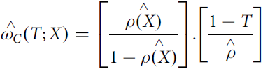 $$\mathop {{\omega _C}}\limits^ \wedge \left( {T;X} \right) = \left[ {{{\mathop {\rho \left( X \right)}\limits^ \wedge } \over {1 - \mathop {\rho \left( X \right)}\limits^ \wedge }}} \right].\left[ {{{1 - T} \over {\mathop \rho \limits^ \wedge }}} \right]$$
where T is either 1 or 0 and indicates whether the individual participates in group A (value 1) or B (value 0);  $\mathop \rho \limits^ \wedge $ is an estimator of the probability that a farmer has accessed rural credit (group A, or T = 1) given the characteristics vector X and may be estimated using a probability model such as Logit or Probit (Chi and Li, Reference Chi and Li2008).
After obtaining the reweighting factors, the RIF regressions for each group can be estimated by OLS:
 $$\mathop {{\beta _t}}\limits^ \wedge = {\left( {\sum\limits_{i \in t} {{\omega _t}.{X_i}.{{X'}_i}} } \right)^{ - 1}}.\sum\limits_{i \in t} {{{\mathop \omega \limits^ \wedge }_t}.\mathop {RIF}\limits^ \wedge } \left( {{y^{ti}};{\upsilon _t}} \right){X_i}$$
for t = A, B and for the counterfactual, the RIF is estimated as:
 $${\mathop \beta \limits^ \wedge {\!_C} = {\left( {\mathop \sum \limits_{i \in A} {{\mathop \omega \limits^ \wedge }_C}\left( {{X_i}} \right).{X_i}.X_i'} \right)^{ - 1}}.\mathop \sum \limits_{i \in A} {\mathop \omega \limits^ \wedge {\!_C}\left( {{X_i}} \right).\mathop {RIF}\limits^ \wedge \left( {{y^{Ai}};{\upsilon _C}} \right){X_i}$$
where the decomposition presented in equation (11) can be obtained as:
 $$\mathop {{\Delta ^\upsilon }}\limits^ \wedge = \left[ {{{\overline X}_B}.\mathop {{\beta _B}}\limits^ \wedge - {{\overline X}_C}.\mathop {{\beta _C}}\limits^ \wedge } \right] + \left[ {{{\overline X}_C}.\mathop {{\beta _C}}\limits^ \wedge - {{\overline X}_A}. \mathop {{\beta _A}}\limits^ \wedge } \right]}_{ \mathop {{\Delta ^\upsilon }}\limits^ \wedge = \mathop {\Delta _R^\upsilon }\limits^ \wedge + \mathop {\Delta _X^\upsilon }\limits^ \wedge $$
We can also identify the contribution of each covariate X k, where k = 1,…, K, on each of the effects obtained in equation (12) as in:
 $$\mathop {\Delta _X^\upsilon }\limits^ \wedge = \mathop \sum \limits_{k = 1}^K \left( {{{\overline X}_{ck}} - {{\overline X}_{Ak}}} \right){\mathop \beta \limits^ \wedge {\!_A}$$
 $$\mathop {\Delta _R^\upsilon }\limits^ \wedge = \left( {{{\mathop \beta \limits^ \wedge }_{B1}} - {{\mathop \beta \limits^ \wedge }_{C1}}} \right) + \mathop \sum \limits_{k = 2}^K {\overline X_{Bk}}\left( {{{\mathop \beta \limits^ \wedge }_{BK}} - {{\mathop \beta \limits^ \wedge }_{CK}}} \right)$$
where in equation (14), the first term (difference in the returns of the covariate k = 1) represents the difference in the intercepts of the regressions of groups A and B, while the second term represents the contribution of the return of each covariate in the total return effect. We used the codes rifreg and oaxaca8 in Stata 14®. In the next section, we present the results obtained using the two methods.
4. Results
In this section, we first present the results of the unconditional quantile regression followed by the results of the income decomposition. Finally, we provide a brief regional analysis of the decomposition of the income differential.
4.1. Influence of rural credit on rural income
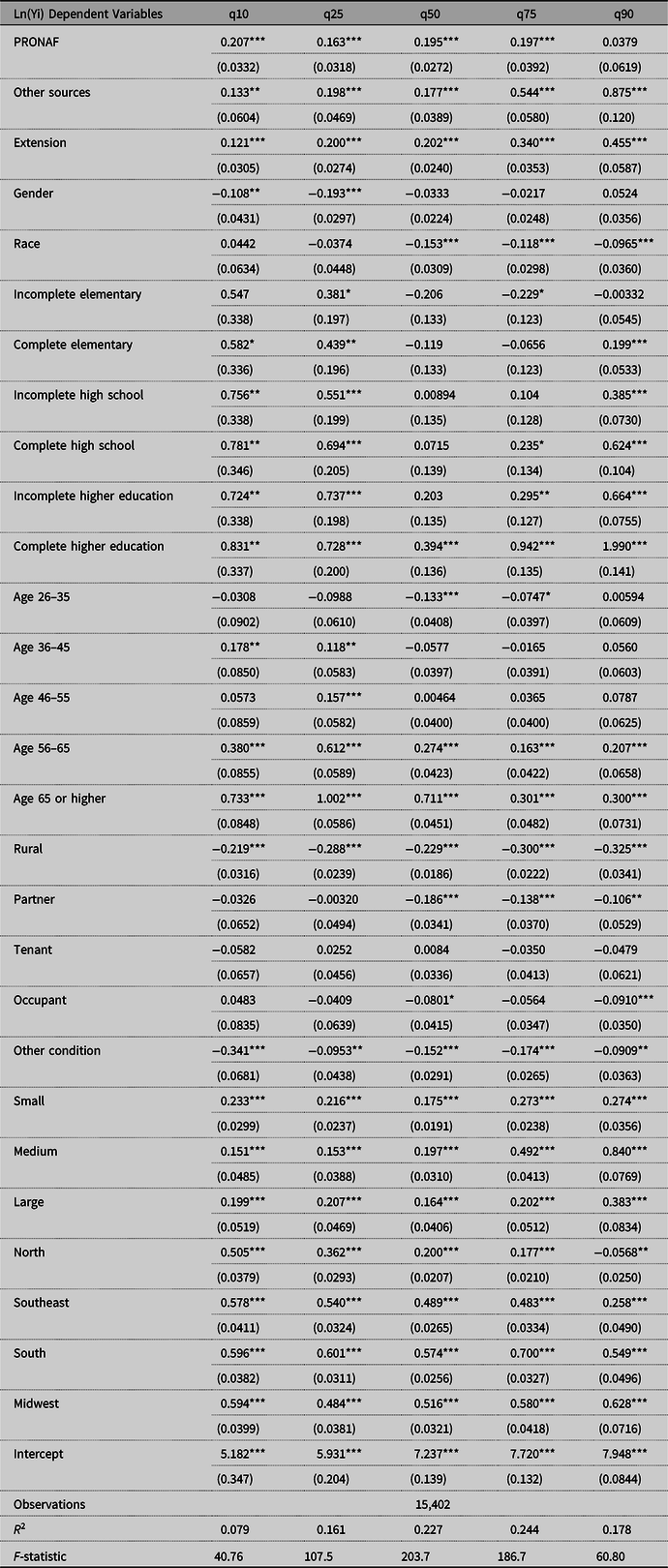
In this section, we present the results of the RIF regressions for the unconditional income distribution quantiles of the logarithm of monthly household income and of the OLS. The estimated coefficients have shown some variations along the income distribution quantiles with respect to the estimated coefficients obtained for the mean (see Figure 2). This result re-enforces the need to use the unconditional quantile regression approach. Table 2 and Figure 2 present the results of RIF regressions for the unconditional income distribution quantiles of the logarithm of monthly household income. Our results suggest households in the bottom two quantiles (q10 and q25) that had access to credit are associated with an income 18.9% (i.e., R$ 94.5 avg.) and 17.2% (i.e., R$ 145.68 avg.) higher than those who did not. This behavior become stronger for the top two quantiles—q75 and q90—at approximately 28.3% (i.e., R$ 805.98 avg.) and 24.6% (i.e., R$ 1,230.00 avg.), respectively.
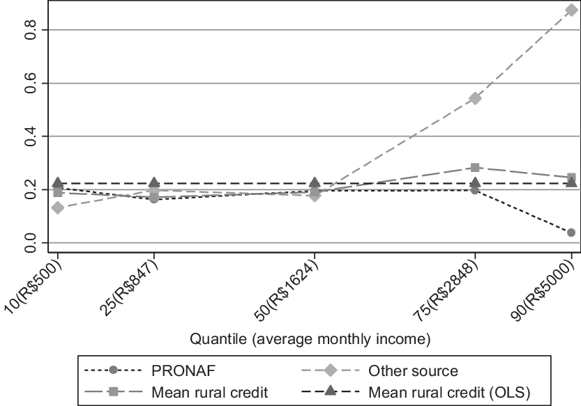
Figure 2. Effects of rural credit on the distribution of income in rural Brazil, 2014.
Table 2. Estimates of unconditional quantile regression, Brazil, 2014

Notes: ***significant at 1%, **significant at 5%, *significant at 10%; standard errors in parentheses; Wald test indicated statistical difference, at a level of 1% of significance, between coefficients of covariates at different monthly income quantiles.
Source: Own elaboration.
These results give us some indications that access to credit can be correlated with monthly household income and income inequality in rural areas of Brazil. It also makes us consider that access to credit is not achieving one of its intended goals. In Brazil, public policies on rural credit availability also aim to raise rural income by providing rural households with the opportunity to acquire more inputs, access new technologies, and reduce market imperfection effects (Alves et al., Reference Alves, Souza and Rocha2013; Leite, Reference Leite2013; Hartarska et al., Reference Hartarska, Nadolnyak and Shen2015; Garcias and Kassouf, Reference Garcias and Kassouf2016).
Variables capturing the effect of gender and race did not show different effects on household income quantiles. We only observed a difference at the bottom of the income distribution, where women have a higher income compared to men. Our results also suggest that household headed by black individuals observe lower incomes compared to other individuals. Experience, represented in this study by the age of the individual, has a stronger influence at the bottom of income distribution.
We found that variables related to a higher level of education (“complete elementary school,” “high school,” and “higher education”) increased household income compared to the base variable (“people who cannot read or write”). Costa et al. (Reference Costa, Costa and Mariano2016), Oliveira and Silveira Neto (Reference Oliveira and Silveira Neto2015), and Reis et al. (Reference Reis, Moreira and Cunha2017) have also identified positive effects of investments in human capital on income. We found that education can decrease income inequality, that is, great income returns to “high school” level in the bottom quantiles of the income distribution. Although “higher education” increases inequality, only 3.2% of the sample has a high education level.
As another public policy associated with agricultural production also observed in this sample, rural extension seeks to generate improvements to farm production and income by helping farmers to access new technologies and knowledge. This policy is traditionally connected with rural credit in Brazil. Our results suggest that access to rural extension is associated with higher income in all quantiles of the distribution. Along the top quantiles of the income distribution, q75 and q90, farmers that had access to rural credit obtained an income 34% and 45.5% higher than the others, respectively.
We found that farm ownership and living in urban areas might lead to higher household incomes. Farm owners have greater incentive to invest in innovations and long-term technologies that contribute to increased rural income. These farmers also have greater access to credit and other services, given that the land can be used as a tangible guarantee for the fulfillment of the financial obligations (Besley, Reference Besley1995). Living in urban areas might lead to greater access to information regarding market input and output, banking institutions, and other services.
Results also suggest that the greater the farm, the greater the income, and that households in the South, Midwest, and Southeast regions are better off compared to households in the North and Northeast (base). These household differences have also been identified in the literature (Assunção and Chein, Reference Assunção and Chein2007; Souza, Ponciano, Ney and Fornazier, Reference Souza, Ponciano, Ney and Fornazier2013; Oliveira and Silveira Neto, Reference Oliveira and Silveira Neto2015; Costa et al., Reference Costa, Costa and Mariano2016).
Access to credit could affect household income differently by source, be it PRONAF or others. To illustrate that, we also estimated the equations disaggregating the variable credit in these two sources. Results are displayed in Table 3 and Figure 2 (which include the average household income per quantile).
Table 3. Estimates of unconditional quantile regression—PRONAF and credit from other sources, Brazil, 2014
Notes: ***significant at 1%, **significant at 5%, *significant at 10%; standard errors in parentheses; Wald test indicated statistical difference, at a level of 1% of significance, between coefficients of covariates at different monthly income quantiles.
Source: Own elaboration.
These results have demonstrated that credit from other sources could be associated with higher rural income, namely by 54.4% (i.e., R$ 1,549.31 avg. in monthly household income quantile q75) compared to farmers that did not have access. It is relevant to point out that PRONAF’s guidelines suggest that this line of credit is designed for low-income families. Also, credit from other sources might provide larger contract values than PRONAFFootnote 10. Thus, comparisons of different sources of credit should consider this point. Access to PRONAF has a steady influence on household income (Figure 2) of approximately 0.2 and a non-significant effect on the top income quantile (due to the lower number of PRONAF borrowers). In summary, households in higher income quantiles experience superior improvements to their incomes when obtaining rural credit (not from PRONAF) compared to those in lower income quantiles. These results suggest the relevance of using the decomposition of income differentials to better understand the factors that explain such variations along the income quantiles.
4.2. Decomposition of income differentials
The data analysis indicates differences in the characteristics of farms with and without access to rural credit. The results presented in the previous subsection also indicate differences in the return to rural credit on income. In this section, we identify which factors explain this difference in income due to access to credit. The income decomposition method is used alongside the RIF regressions to evaluate how much of the income differences observed between the farm groups is attributed to the composition effect and return effect. The former effect represents differences in the distribution of the individuals’ characteristics, while the latter represents differences in the returns of these characteristics. It allows us to identify the contribution of each explanatory variable on each of the estimated effects. The outcome of this methodology is presented in Table 4 and summarized in Figures 3, 4, and 5.
Table 4. Decomposition of the income differentials: with rural credit and without rural credit, Brazil, 2014

Note: #Includes Gender and Race.
Source: Own elaboration.
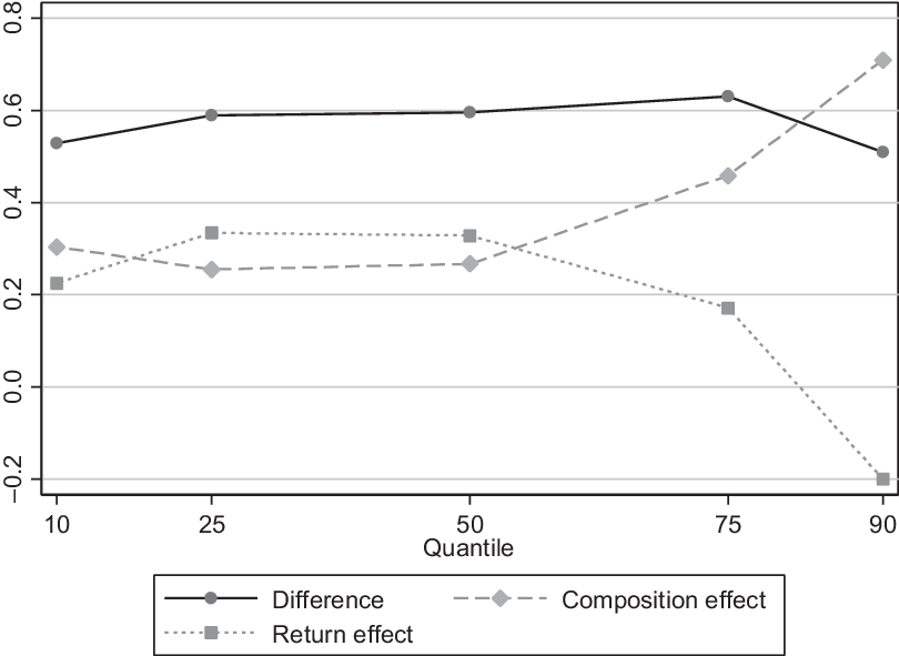
Figure 3. Decomposition of the income differential: with rural credit and without rural credit, Brazil, 2014.
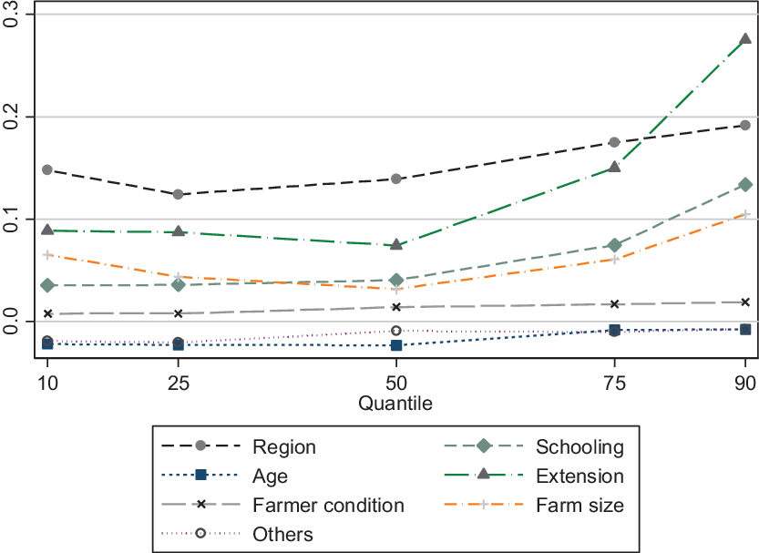
Figure 4. Detailed decomposition of the composition effect of income differential, Brazil, 2014.

Figure 5. Decomposition of the income differential: With rural credit—without rural credit, selected regions, Brazil, 2014.
Rural households (farms) that had access to rural credit obtained a positive income gain in all the quantiles considered compared to farmers that did not have access to these services (Figure 3). Overall, the composition effect governs the income differential in the income quantiles q10 and from q50 and above. This implies that the differences in individual characteristics such as schooling and access to rural extension explain nearly the entire income gap in these quantiles, especially from q75 and above (see Figure 4).
The return effect is steady over the distribution, except along the top quantiles. This implies that, for the top quantiles, the income differential is not explained by the difference on the return (effect on income) of household characteristics between those that had access to credit and those that did not, that is, for income quantiles lower than q75, the return effect is positive, which suggests that households that had access to credit obtained a higher return to household/individual characteristics on their income, such as education.
Figure 4 and Table 4 break down the composition effect. We found that access to rural extension, education, and the location of residence are the main factors explaining the higher level of income for farmers that had access to rural credit. This suggests a potential selection bias on the provision of rural credit, including PRONAF, which was also pointed out by Aquino and Schneider (Reference Aquino and Schneider2011). The negative influence of age and other characteristics (e.g., gender and race) indicate that these variables contribute to the reduction of income differential between farmers that had access to credit and those that did not. These results suggest that the effect of credit might be constrained for low-income farmers given the lack of education and access to rural extension. Higher education level also helps farmers to absorb information and implement technical recommendations more precisely (Freitas, Reference Freitas2017).
We also break down the return effect to better understand how the return to the characteristics affects household income (see Table 4). Although we observed an erratic influence of schooling on rural income, this variable contributes considerably to income in the two highest income quantiles (q75–q90). This result might be associated with the lower presence of farmers with high schooling levels in these quantiles, which leads to a higher return for this variable (marginal effect). The exact opposite is true for the lowest quantiles (q10–q50). In general, most of the variables have a similar influence on income differentials.
4.3. Regional analysis
Regional disparities remain a strong factor in Brazilian rural areas, as suggested by Azzoni (Reference Azzoni2001), Alves et al. (Reference Alves, Souza and Rocha2013), and Costa et al. (Reference Costa, Costa and Mariano2016). Figure 5 presents regional differences in income gap focusing on the return effect—the most prominent influence in the comparison between the regions. The models were re-estimated for selected pairs of Brazilian regions. The results suggest that a household in the Northeast region would obtain a much greater income effect from access to credit if they had the same characteristics as households in the Southeast, though not necessarily with a reduction in income inequality. A similar trend was observed in the comparison between the Northeast and South regions: if Northeastern farmers had the same characteristics as Southern farmers, they would obtain a greater income but now with an important influence of decreasing income inequality in Northeastern rural area.
5. Concluding remarks
The Brazilian agriculture segment has been growing exponentially in recent decades and has expanded its international market participation. However, Brazil continues to face a high level of rural inequality. In this paper, we sought to identify whether access to credit deepens or reduces inequality among rural households in Brazil. To obtain the effect of credit on household income, we used an income decomposition proposed by Firpo et al. (Reference Firpo2007) and the household survey of 2014 from the IBGE (National Household Sample Survey—PNAD).
Our results suggested that Brazilian rural credit policy was capable of increasing rural household income in all income quantiles, but this also increased income inequality. However, we observed a smaller influence of PRONAF on increasing inequality. Additionally, we found that the rural credit from other sources has a greater effect on rural income in the top income quantiles. An income differential decomposition has demonstrated that the difference in individual characteristics explains most of the income differential in the upper portion of the income distribution.
The results of the present study indicate that a higher level of education and access to rural extension may be associated with a greater influence of rural credit on household income, which implies that access to rural credit alone cannot raise the social welfare of low-income farmers. Our findings suggest that the design of a joint public policy incorporating rural credit, rural extension, and the promotion of human capital would have much a stronger effect on reducing income inequality in the rural areas of Brazil. This suggests the existence of synergy between public policies and public services linked to rural credit.
Additionally, it is important to note that the Northeast region of Brazil should receive greater focus in the context of receiving beneficial extension services and human capital increase policies. This would allow its farmers to perform similarly to farmers in the South and Southeast regions, which would boost the result of rural credit programs in this region.
Financial disclosure
This was supported by Climate Policy Initiative (CPI) in Brazil through a seed grant under the Land Use Initiative (Iniciativa pelo Uso da Terra—INPUT).
Conflicts of interest
None.


 Open access