


1. Introduction
This article is concerned with a variant of the isoperimetric problem, for which we investigate the optimal energy of an elastic inclusion of a fixed volume. Here the energy consists of an interfacial and a geometrically nonlinear elastic contribution. The latter is defined by an integral of the stored-energy density function over a domain. As usual, the stored-energy density depends on the strain and describes properties of the material. Physically, the problem is motivated by nucleation phenomena which arise, for instance, in shape-memory materials [Reference Bhattacharya9].
The set-up considered in this work is the geometrically nonlinear analogue of [Reference Knüpfer and Kohn42] where the isoperimetric problem for a geometrically linear elastic two-phase inclusion problem had been investigated. Our main aim is to deduce quantitative information on the nucleation problem by studying its scaling properties. The problem of determining the sharp form of the inclusion seems to be more complicated [Reference Müller60]. In addition to the presence of non-quasiconvexity as in [Reference Knüpfer and Kohn42], in the geometrically nonlinear setting under investigation, an additional difficulty is present in the form of the nonlinear gauge group ${\rm SO}(2)$ . We emphasize that nonlinear models are more general than linear ones and, therefore, should be considered primarily. Linearized elasticity correctly describes only very particular deformations that are close to elastic equilibria (cf. [Reference Bhattacharya8] for a comparison of the two theories). In order to deal with the nonlinear structure of the model, we hence rely on the geometrically nonlinear rigidity result from [Reference Conti and Schweizer28] in combination with the ideas from [Reference Knüpfer and Kohn42].
1.1 Model and statement of results
We consider the interior nucleation of a new phase in an elastic material in two space dimensions. More specifically, we consider a material for which two different phases (lattice structures) are energetically preferred. These are represented by the ${\rm SO}(2)$ orbit of the identity matrix $\operatorname {Id} \in \mathbb {R}^{2 \times 2}$
 and the ${\rm SO}(2)$
 orbit of another matrix $F \in \mathbb {R}^{2 \times 2}\backslash {\rm SO}(2)$
 . The deformation of the material is described by a function $v : \mathbb {R}^2 \to \mathbb {R}^2$
 . By the Cauchy–Born rule the energy of an elastic material can be represented in terms of the gradient of the deformation function $v$
 . Following the phenomenological theory of martensite and assuming Hooke's law, we study (volume-constrained) minimizers of the energy

Here $\chi : \mathbb {R}^2 \rightarrow \{ 0 , 1 \}$ encodes the location of the new, minority phase. Its variation i.e. the first integral in (1.1) is the interfacial energy, while the second integral is the elastic energy. Hence, our model includes penalizations of transitions between the phases and deviations from the corresponding material phase. We introduce $\mu >0$
 to denote the volume of the inclusion

for the region $M:=\{x\in \mathbb {R}^2: \ \chi (x)=1\}$ associated with the minority phase. In what follows, we will consider minimizers of the energy (1.1) for a prescribed volume of the minority phase. In order to rule out self-intersections, as the set ${\mathcal {A}}_m$
 of admissible functions we consider

Here bi-Lipschitz with constant $m\geq 1$ means that $v$
 is a homeomorphism and $v$
 and $v^{-1}$
 are Lipschitz continuous functions with Lipschitz constants $m\geq 1$
 . Seeking to model nucleation phenomena, we assume that the strain $F$
 is compatible with the identity matrix. In two dimensions this is equivalent to the condition $\det F = 1$
 . Our main result is the scaling of the minimal energy for prescribed inclusion volume:
Theorem 1.1 (Scaling of ground-state energy)
Suppose that $F \in \mathbb {R}^{2 \times 2}\backslash {\rm SO}(2)$ satisfies $\det F = 1$
 . Let $\mu$
 be as in (1.2). Let $m \geq \max \{ \|F\|_{}, \|F^{-1}\|_{} \} + C$
 for some sufficiently large constant $C>0$
 . Then for any $\mu >0$
 we have

Here, we write $A \sim B$ by which we mean that $cA \leq B \leq CB$
 for two constants $c,C > 0$
 which are independent of $\mu$
 but may depend on $F$
 . The first bound in Theorem 1.1 corresponds to the usual isoperimetric regime in which the surface energy dominates while the second estimate for $\mu \geq 1$
 captures the effect of the interaction of the surface and elastic energies. In particular, the role of anisotropy in the elastic contribution in the form of the two physical phenomena of compatibility and self-accommodation are captured in it. We do not track the dependence on $\| F\|$
 in the energy scaling behaviour.
The result of theorem 1.1 confirms the similar scalings which had been obtained in the framework of piecewise linear elasticity in [Reference Knüpfer and Kohn42]. In particular, the result shows that in the framework of geometrically nonlinear elasticity, the model imposes enough rigidity to ensure the same lower bound on the energy as in the geometrically linear model. This is in line with the fact that the only solution for the two-gradient problem for two compatible strains are twins in nonlinear elasticity theory [Reference Ball and James3, proposition 2] as well as in linear elasticity theory. If we allow for more variants of martensite, the situation is expected to become more intricate since in this case the corresponding many gradient problems possibly allow for a large number of non-trivial solutions and complicated microstructure [Reference Bhattacharya9, Reference Müller60].
1.2 Ideas of the proof
The proof of our main result can be split into two parts: an ansatz-free lower-bound estimate and an upper-bound construction.
On the one hand, in order to verify the lower bound, we observe that without loss of generality, we may assume the deformation $F$ to be symmetric and positive-definite after using the polar decomposition theorem. By a suitable choice of coordinates, $F$
 hence takes the form

With these normalization results on hand, in the small volume regime, the lower bound follows by the standard isoperimetric inequality. In the large volume setting, we deduce the lower bound by a combination of a segment rigidity argument from [Reference Conti and Schweizer28] (§ 2) and the localization argument from [Reference Knüpfer and Kohn42] (§ 4.1). Working with phase indicator energies as in [Reference Knüpfer and Kohn42] or [Reference Capella and Otto13], see (1.1), contrary to the energies in [Reference Conti and Schweizer28], we do not directly control the full second derivatives of the deformation $v$ . This additional degeneracy results in a number of small adaptations becoming necessary. For settings with full second-derivative control the key localized energy estimate in proposition 3.1 would directly follow from corollary 2.5 in [Reference Conti and Schweizer28]. Moreover, in this case also the higher-dimensional problem could be treated directly in parallel by invoking the results from [Reference Chermisi and Conti19] or [Reference Jerrard and Lorent37]. With our energies this would require adaptations of these strategies, e.g. in the associated rigidity results, which we do not pursue in the present article. The slightly stronger degeneracy of our energy which does not immediately yield the full second-derivative control, also accounts for one of the technical reasons for our bi-Lipschitz assumptions in the minimization problem; another reason being the use of approximation theory for bi-Lipschitz functions in § 3. Although more general deformations might be possibly considered at the expense of various technical difficulties, we would like to emphasize that bi-Lipschitz deformations automatically guarantee injectivity everywhere, that is essential in mathematical elasticity. Results ensuring almost everywhere injectivity rely on Hölder continuous deformations and orientation-preserving maps [Reference Ciarlet and Nečas23]. Additional control of the distortion is needed if we want to achieve injectivity everywhere [Reference Hencl and Koskela36].
On the other hand, the upper bound is derived by constructing a deformation $v$ corresponding to a well-known construction for a lens-shaped elastic inclusion (see e.g. [Reference Knüpfer and Kohn42]) which in our geometrically nonlinear setting leads to an orientation-preserving deformation.
1.3 Relation to the literature
Due to their physical significance and the intrinsic mathematical interest in ‘non-isotropic’ isoperimetric inequalities, nucleation problems for shape-memory materials have been studied in various settings: in a geometrically linearized framework the compatible and incompatible two-well problems (one variant of martensite and one variant of austenite) have been considered in [Reference Knüpfer and Kohn42], where a localization strategy was introduced. This also forms one of the two core ingredients of our result. Moreover, the nucleation behaviour for the geometrically linearized cubic-to-tetragonal phase transformation was studied in [Reference Knüpfer, Kohn and Otto43] in which Fourier theoretic arguments in the spirit of [Reference Capella and Otto12, Reference Capella and Otto13] were exploited. Fourier theoretic arguments also underlie the study of the nucleation of multiple phases without gauge invariance in [Reference Rüland and Tribuzio65]. Using related ideas, the nucleation behaviour at corners of martensite in an austenite matrix was investigated in [Reference Bella and Goldman6]. We also refer to [Reference Ball and Koumatos4, Reference Ball, Koumatos and Seiner5, Reference Kružík53] for the study of quasiconvexity at the boundary. Further, highly symmetric, low-energy nucleation mechanisms have been explored in [Reference Cesana, Della Porta, Rüland, Zillinger and Zwicknagl16, Reference Conti, Klar and Zwicknagl27] both in the geometrically linear and nonlinear theories in two dimensions. In the geometrically nonlinear settings substantially less is known in terms of nucleation properties due to the presence of the nonlinear gauge group. In this context, the incompatible two-well problem was studied in [Reference Chaudhuri and Müller18] in which an incompatible two-well analogue of the Friesecke–James–Müller rigidity result [Reference Friesecke, James and Müller35] was used. Moreover, the study of model singular perturbation problems for the analysis of austenite–martensite interfaces in terms of a surface energy parameter [Reference Kohn and Müller49, Reference Kohn and Müller50] laid the basis for an intensive, closely related research on singular perturbation problems for shape-memory alloys [Reference Chan and Conti17, Reference Chipot, Collins and Kinderlehrer20, Reference Chipot and Müller21, Reference Conti, Diermeier, Melching and Zwicknagl24, Reference Conti and Schweizer28, Reference Conti and Zwicknagl29, Reference Davoli and Friedrich31, Reference Lorent56, Reference Rüland63, Reference Rüland and Tribuzio64, Reference Rüland and Tribuzio66, Reference Zwicknagl68]. Contrary to the full nucleation problems, in these settings the phenomenon of compatibility plays the main role, while nucleation phenomena in addition require the analysis of the phenomenon of self-accommodation. Moreover, dynamic nucleation results have been considered in [Reference Della Porta32, Reference Della Porta, Rüland, Taylor and Zillinger33, Reference Kružík, Mielke and Roubíček54]. We refer to [Reference Kružík and Roubíček55, Reference Müller60] for further references on these and related results.
Nonlocal isoperimetric inequalities have also been investigated for the Ohta–Kawasaki energy and related models with Riesz interaction. For example, we refer to [Reference Alama, Bronsard, Topaloglu and Zuniga1, Reference Bonacini and Cristoferi10, Reference Bonacini, Knüpfer and Röger11, Reference Frank and Lieb34, Reference Julin38, Reference Julin39, Reference Knüpfer and Muratov45, Reference Knüpfer and Muratov46, Reference Lu and Otto57]. In these models, above a critical volume minimizers do not exist anymore and the scaling of the energy in terms of the mass is linear. Other related vectorial models where the energy includes both interface type energies as well as a (dipolar) nonlocal interaction are ferromagnetic systems. The nucleation of magnetic domains during magnetization reversal and corresponding optimal magnetization patterns have been investigated in [Reference Knüpfer and Muratov44, Reference Knüpfer and Nolte47, Reference Knüpfer and Stantejsky48], see also [Reference Otto and Viehmann61]. The competition between a nonlocal repulsive potential and an attractive confining term is found also in other problems, for example in models studying the interaction of dislocations [Reference Kimura and van Meurs41, Reference van Meurs67] or [Reference Carrillo, Mateu, Mora, Rondi, Scardia and Verdera14, Reference Carrillo, Mateu, Mora, Rondi, Scardia and Verdera15, Reference Mora, Rondi and Scardia59]. Another anisotropic and nonlocal repulsive energy that has been treated variationally using ansatz-free analysis is discussed in [Reference Carrillo, Mateu, Mora, Rondi, Scardia and Verdera15] (based on [Reference Carrillo, Mateu, Mora, Rondi, Scardia and Verdera14, Reference Mora, Rondi and Scardia59]). We finally briefly mention investigations of other physical settings where related nonlocal isoperimetric inequalities have been studied. This includes the works [Reference Kohn and Wirth51, Reference Kohn and Wirth52, Reference Potthoff and Wirth62] on compliance minimization, on epitaxial growth (e.g. [Reference Bella, Goldman and Zwicknagl7]), on dislocations (e.g. [Reference Conti, Garroni and Ortiz25]) and superconductors (e.g. [Reference Choksi, Conti, Kohn and Otto22, Reference Conti, Goldman, Otto and Serfaty26]). We emphasize that the above list of references is far from exhaustive.
1.4 Notation
We write $A \lesssim B$ if $A \leq C B$
 for some constant $C$
 which is independent of $\mu$
 , but may, for instance, depend on $F$
 . The Frobenius norm of a matrix $A\in \mathbb {R}^{d\times l}$
 is denoted by $\|A\|=\sqrt {\operatorname {tr}(A^tA)}$
 . For two matrices $A,B$
 we write ${\rm dist}(A,B) := \|A-B\|_{}$
 , where $\|\cdot \|_{}$
 is the Frobenius norm, analogously, we define ${\rm dist}(A,{\mathcal {K}}) := {\rm dist}_{K \in {\mathcal {K}}}(A,K)$
 for any ${\mathcal {K}} \subset \mathbb {R}^{2 \times 2}$
 .
.
By $B_R(x)$ we denote the ball of radius $R>0$
 centred at $x \in \mathbb {R}^2$
 and we write $B_R := B_R(0)$
 . We write $M:={\rm spt}\,\chi \subset \mathbb {R}^2$
 to denote the support of the minority phase. For $E\subset \mathbb {R}^2$
 and $v \in BV(E)$
 , the total variation of $v$
 is denoted by $\|\nabla v\|_E$
 .
.
2. Rigidity
The aim of this section is to find a ‘good’ set in the shape of a rhombus which fulfils a variant of the rigidity estimate from [Reference Conti and Schweizer28]. We first introduce some notation for the elastic energies for the deformation $v$ . We set

Then the elastic energy for a one-dimensional (1D) or two-dimensional subset $E \subset \mathbb {R}^2$ is defined as

and the total elastic energy is ${\mathcal {E}}_{\rm elast}[\chi, v] := {\mathcal {E}}_{\rm elast}[\chi, v,\mathbb {R}^2]$ . Similarly, we introduce

which we will use in order to deal with estimates for the inverse of $v$ . If the subset is 1D we integrate over the 1D Hausdorff measure instead of the Lebesgue measure.
Before stating the central rigidity estimate, we formulate two auxiliary lemmas. First, we note that there is a large set of non-singular points:
Lemma 2.1 (Non-singular points)
Let $f \in L^1(B_R)$ and $R>0$
 . Then for any $\theta > 0$
 there is $U \subset B_R$
 with $|B_R \backslash {U}| < \theta$
 and a constant $C = C(\theta )>0$
 such that for any $x_0 \in U$
 we have

Proof. This follows by an application of Fubini's theorem and since ${\rm dist}^{-1}{(\cdot,x_0)} \in L_{\rm loc}^1$ .
.
By our bi-Lipschitz assumption, bounds on $v$ can be translated into analogous bounds for its inverse:
Lemma 2.2 Let $R>0$ , $m\geq 1$
 and let $(\chi, v)\in {\mathcal {A}}_m$
 with $v(0)=0$
 and $v\in C^1(B_{mR})$
 . Assume that

Then for $\chi _1 :=\chi \circ (v^{-1})$ we have
(i) $\displaystyle {\|\chi _1\|_{L^{1}(B_{R})}} \leq m^2 \eta R^2;$

(ii) $\displaystyle \|\nabla (\chi _1)\|_{B_{R}} \leq m \eta R;$
(iii) $\displaystyle {\mathcal {E}}'_{\rm elast}[\chi _1, v^{-1}, B_R] \leq C {\mathcal {E}}_{\rm elast}[\chi, v, B_{mR}]$
for some constant $C=C(m, F)>0$.


Proof. By the transformation formula and since $v \in {\mathcal {A}}_m$ , (i) follows from

By the chain rule for BV functions (cf. theorem 3.16 in [Reference Ambrosio, Fusco and Pallara2]) this implies

The claim of (iii) follows by an application of the linear algebra fact from lemma A.2(ii). Indeed, using the pointwise identity

together with the inverse function theorem, the transformation theorem and with the notation $\tilde v := v^{-1}$ , we arrive at

for some constant $C=C(m, F)>0$ . This completes the proof.
We are now ready to give the key rigidity estimate. It is a variant of the two-well rigidity estimate from [Reference Conti and Schweizer28] and shows that we can find a sufficiently large rhombus such that we control the energy and the change of length on all six connecting lines between the corner points of this rhombus both for the transformation and its inverse:
Lemma 2.3 (Rigidity estimate): Let $R>0$ , $m\geq 1$
 , $\delta \in (0, R/{m})$
 . Then there are constants $\eta =\eta (\delta )>0$
 and $C = C(\delta,m,F)>0$
 such that the following holds: assume $(\chi, v)\in {\mathcal {A}}_m$
 satisfies $v\in C^1(\overline {B_R},\mathbb {R}^2)$
 ,
,

Then there exist four points ${\mathcal {C}} := \{ a, b, c, d \} \subset B_{{R}/{m}}\subset \mathbb {R}^2$ with $|a-b| \sim R/m$
 and $|c-d| \sim \delta R/m$
 , which form the end-points of a symmetric rhombus $T$
 such that for all $x,y\in {\mathcal {C}}$
 and with the notation $M = spt\, \chi$
 we have the following properties:
(i) $\displaystyle [x, y] \cap M = \emptyset$
;(ii) $\displaystyle {\mathcal {E}}_{\rm elast}[\chi,v,[x, y]] \leq \ \frac {C}{R} {\mathcal {E}}_{\rm elast}[\chi, v,B_R]$
;(iii) $\displaystyle \int _{B_R} e_{\rm {elast}}(\chi, v) \frac {{\rm d}z}{{\rm dist}(z,x)} \leq \frac {C}{R} {\mathcal {E}}_{\rm elast}[\chi, v, B_R]$
.


Furthermore, for $\chi _1 :=\chi \circ (v^{-1})$ we have
(iv) $\displaystyle [v(x), v(y)] \cap v(M) = \emptyset$
;(v) $\displaystyle {\mathcal {E}}_{\rm elast}'[\chi _1,v^{-1},[v(x), v(y)]] \leq \frac {C}{R} {\mathcal {E}}_{\rm elast}'[\chi _1, v^{-1},B_R]$
;(vi) there exist $Q\in {\rm SO}(2)$
and $p\in \mathbb {R}^2$ such that
\[ |v(x)-Qx-p|\leq C({\mathcal{E}}_{\rm elast}[\chi, v, B_R]^{1/2}+\eta^{1/2}). \]
Finally, we have rigidity on all six segments
(vii) $\displaystyle \left | 1 - \frac {|v(x)-v(y)|}{|x-y|} \right | \leq \ \frac {C}{R} {\mathcal {E}}_{\rm elast}[\chi, v, B_R]^{ 1/2}$
.


Proof. Without loss of generality, by scaling, we may assume that $R=m$ and $v(0)=0$
 . We further choose $\theta \in (0,1)$
 sufficiently small to be determined below. We argue in several steps based on averaging-type arguments.
Step 1: Identification of a symmetric cross satisfying (i) and (ii). We first construct horizontal and vertical segments forming a ‘cross’ satisfying (i) and (ii). For $\delta \in (0, 1/2)$ and $r \in (-\delta, \delta )$
 we define the horizontal line segment by $L_{\rm hor}(r) =[p_{-}(r),p_+(r)] \subset B_1$
 where $p_{\pm }(r):=(\pm 1/2,r)$
 . We first show that if $\eta >0$
 is sufficiently small, there exists a subset $E \subset (-\delta,\delta )$
 of volume fraction $1-\theta$
 such that

Indeed, for some $C=C(\delta, \theta )>0$ , we define

By Chebyshev's inequality and in view of (2.3) we have

by choosing $\eta = \eta (\delta,\theta )$ sufficiently small and $C = C(\delta,\theta )$
 sufficiently large. In particular, $|E| \geq 2\delta (1-\theta )$
 . Now, since for each $r\in E$
 , $\nabla \chi |_{L_{\rm hor}(r)}$
 is a discrete measure and since $\theta \in (0, 1)$
 , this implies $\nabla \chi |_{L_{\rm hor}(r)} = 0$
 for all $r\in E$
 . By definition of $E$
 we then have $\chi _{|L_{\rm hor}(r)} = 0$
 for $r \in E$
 (cf. [Reference Knüpfer and Kohn42, p. 701]). This shows that outside of volume fraction $\theta$
 , the horizontal segments $L_{\rm hor}(r)$
 have properties (i)–(ii).
Next, we repeat this argument along the vertical lines of the form $L_{\rm ver}(s)=[q_{-}(s),q_+(s)]$ with $q_{\pm }(s)=(s,\pm \delta )$
 for $s\in [-1/2, 1/2]$
 . Also for this set, we analogously find a volume fraction $\tilde {E}\subset [-1/2,1/2]$
 of size $1-\theta$
 such that these vertical line segments satisfy (i)–(ii).
Consider now the sets $\{L_{\rm hor}(r)\}_{r\in E}$ and $\{L_{\rm ver}(s)\}_{s\in \tilde {E}}$
 of all horizontal and vertical segments with properties (i)–(ii), respectively (see figure 1). Let $o(s,r) =L_{\rm hor}(r) \cap L_{\rm ver}(s)$
 be the intersection point of the corresponding horizontal and vertical line. The point $o(s,r)$
 divides both $L_{\rm hor}(r)$
 and $L_{\rm ver}(s)$
 into two segments denoted by $L_{\rm hor}^+(r)$
 and $L_{\rm hor}^-(r)$
 (also $L_{\rm ver}^+(s)$
 and $L_{\rm ver}^-(s)$
 ). Since $E$
 and $\tilde {E}$
 are sets of positive (close to one) volume fractions, there exist $r_0\in E$
 and $s_0\in \tilde {E}$
 such that $|L_{\rm hor}^+(r_0)|\sim |L_{\rm hor}^-(r_0)|$
 and $|L_{\rm ver}^+(s_0)|\sim |L_{\rm ver}^-(s_0)|$
 . Consequently, we choose $L_{\rm hor}'$
 and $L_{\rm ver}'$
 such that $o=L_{\rm hor}(r_0)\cap L_{\rm ver}(s_0)$
 is the midpoint of $L_{\rm hor}'$
 as well as the midpoint of $L_{\rm ver}'$
 . This can be done by (if necessary) cutting exceeding parts of $L_{\rm hor}(r_0)$
 and $L_{\rm ver}(s_0)$
 ; we note that such a modification preserves the conditions $|L_{\rm hor}'|\sim 1$
 and $|L_{\rm ver}'|\sim \delta$
 .
.
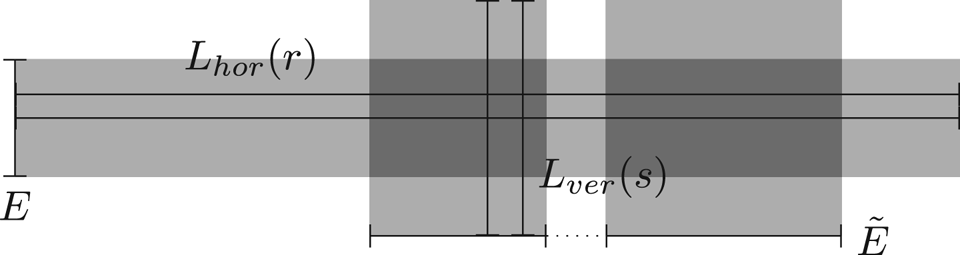
Figure 1. Grey rectangles represent sets of horizontal and vertical segments with properties (i)–(ii).
Step 2: Identification of a ‘good’ rhombus. Let $L_{\rm hor}'$ and $L_{\rm ver}'$
 be the segments forming a symmetric cross and satisfying (i)–(ii) as in the previous step. Let $\hat T$
 be the symmetric rhombus given by the convex hull of this cross. We denote by $\hat {T}_\rho$
 the homothetically shrunken rhombus with the self-similarity factor $\rho \in (0,1]$
 and the same centre point. For $\rho \in ({1}/{4},{3}/{4})=:I$
 , the diagonals (given by the corresponding shortened line segments of the originally constructed cross) of the resulting symmetric rhombi $\hat T_\rho$
 also satisfy (i)–(ii) by construction, see figure 2. After using a Fubini argument as in step 1, we obtain a subset $I_1$
 of $I$
 on which all sides of the rhombus fulfil properties (i)–(ii).
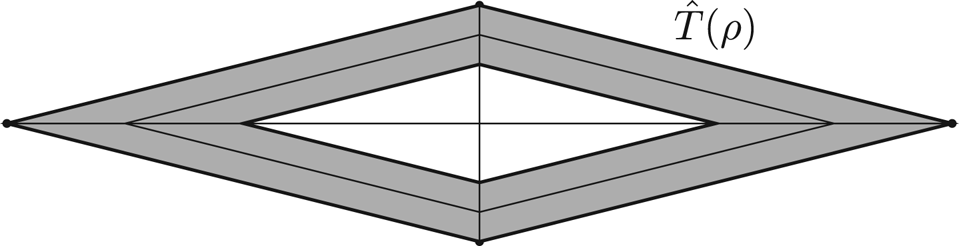
Figure 2. Sketch of a set of rhombi $\hat {T}(\rho )$ , $\rho \in ({1}/{4},{3}/{4})$
 .
.
Next, we seek to ensure that properties (iii)–(v) are also satisfied on the edges of some of these rhombi. Invoking lemma 2.1 together with another averaging argument, we obtain another set $I_2\subset I$ of positive volume fraction satisfying (iii). In addition to this, since $v$
 is bi-Lipschitz and by lemma 2.2(i)–(ii), we can repeat step 1 with the functions $v^{-1}$
 and $\chi _1$
 , the energy ${\mathcal {E}}'_{\rm elast}[\chi _1,v^{-1},B_m]$
 and for the line segments $[v(x),v(y)]$
 , where $x,y$
 form the endpoints of the rhombi $\hat T_\rho$
 for $\rho \in I$
 . Thus, noting that by the bi-Lipschitz property of $v$
 , the length of the lines $[v(x),v(y)]$
 is (up to a factor $m, m^{-1}$
 ) comparable to that of $[x,y]$
 and after possibly enlarging the constant $C>0$
 , we obtain a subset $I_3$
 of $I$
 with properties (iv)–(v). By choosing the intersection of these subsets of $I$
 , we arrive at a subset of $I$
 with positive volume fraction such that all sides of $\hat {T}_{\rho }$
 fulfil (i)–(v) for $\rho$
 in this subset, provided $\eta >0$
 is sufficiently small.
By the Friesecke–James–Müller rigidity theorem [Reference Friesecke, James and Müller35] and Poincaré's inequality, there exist $Q\in {\rm SO}(2)$ and $p\in \mathbb {R}^2$
 such that for constants $C_{\delta }, C_{F}>0$
 , we have

Again, the use of a Fubini argument implies that there are many values of $\rho$ such that the resulting rhombi $\hat {T}_\rho$
 are ‘good’, in the sense that all lines connecting the corner points of the rhombus satisfy properties (i)–(v) and that for some constant $C=C(F,\delta )>0$
 we have

Then by Sobolev's embedding theorem, we obtain

We choose one such ‘good’ rhombus and denote it by $T$ and define its endpoints as the points ${\mathcal {C}} := \{ a,b,c,d \}$
 (see figure 3). Since $v$
 is a continuous function, we obtain from inequality (2.4)

As a consequence, by construction properties (i)–(vi) are satisfied for these endpoints.
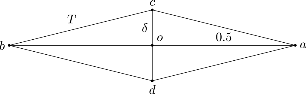
Figure 3. Sketch of the rhombus $T$ constructed in lemma 2.3.
Step 3: Proof of (vii). By the fundamental theorem of calculus, for any $x,y \in {\mathcal {C}}$ we have

Now, we apply the same argument to $v^{-1}(v(x))-v^{-1}(v(y))$ with $x,y \in {\mathcal {C}}$
 . Thus, in view of lemma 2.2, for a constant $C=C(\delta, m, F)>0$
 we obtain

Combining inequalities (2.5) and (2.6), we obtain the desired estimate (vii). This completes the proof of the lemma.
3. A lower bound for the elastic energy
In this section, we prove a local lower bound by exploiting the rigidity argument from lemma 2.3 and the ideas from the proof of lemma 2.3 in [Reference Conti and Schweizer28]. This local lower bound provides a geometrically nonlinear variant of the central lower bound from proposition 3.1 in [Reference Knüpfer and Kohn42]. In § 4.1 we will combine it with a covering argument as in [Reference Knüpfer and Kohn42] which will imply the lower bound of theorem 1.1.
Proposition 3.1 (Lower bound on elastic energy)
There is $\eta > 0$ such that for any $R > 0$
 the following holds: suppose that $(\chi, v)\in {\mathcal {A}}_m$
 satisfies

Then there are constants $\alpha = \alpha (m) \in (0,1)$ and $C = C(F,\alpha,m)>0$
 such that

Proof. This result essentially follows from an application of a variant of the two-well rigidity result from [Reference Conti and Schweizer28]. Here there are slight adaptations in steps 1 and 2 in the proof due to the choice of our energies (full gradient control in [Reference Conti and Schweizer28] vs. our phase-indicator energies), while steps 3 and 4 then follow essentially without changes as in [Reference Conti and Schweizer28]. For self-containedness, we repeat the argument for proposition 3.1.
By scaling we can assume $R=m$ and by the approximation results in [Reference Daneri and Pratelli30] for bi-Lipschitz functions we can further assume that $v \in C^1(\overline {B_m})$
 .
.
Following the argument in [Reference Conti and Schweizer28] in our proof we will construct a rhombus $T$ with $B_\alpha \subset T \subset B_1$
 and show that the corresponding estimate (3.1) holds for $T$
 replaced by $B_\alpha$
 for some $\alpha > 0$
 . We write $\mu := {\|\chi \|_{L^{1}(B_{\alpha })}}$
 and $\epsilon := {\mathcal {E}}_{\rm elast}[\chi,v,B_m]$
 . Moreover, we note that, without loss of generality, we can assume

Indeed, if $\epsilon$ is large e.g. $\epsilon ^{1/2}\geq \eta$
 , then by assumption we have $\|\chi \|_{L^1(B_1)}\leq \eta \leq \epsilon ^{1/2}$
 . Then inequality (3.1) follows immediately.
Step 1: Construction of a ‘good’ rhombus. Since $F \neq \operatorname {Id}$ and $\det F = 1$
 after a rotation of coordinates, we may assume that $|Fe_1|<1$
 . Hence, there exists $\delta >0$
 such that

Without loss of generality we can assume that $\delta \in (0, 1)$ so that the conditions of lemma 2.3 with $R = m$
 are satisfied. We then consider a rhombus $T$
 with corner points ${\mathcal {C}} := \{ a, b, c, d \}$
 as obtained in lemma 2.3, see figure 3. Since $|c-d|\sim \delta$
 and $|a-b| \sim 1$
 , in particular,

By lemma 2.3 we further have properties (i)–(vii) for this rhombus.
Step 2: We claim that there exist $Q\in {\rm SO}(2)$ and $p \in \mathbb {R}^2$
 such that $v(x)$
 is close to $Q x + p$
 for any point $x\in {\mathcal {C}}$
 up to an error of order $\epsilon ^{1/2}$
 . Indeed, by lemma 2.3(vii) the six lengths $|x-y|$
 for $x,y\in {\mathcal {C}}$
 are preserved by $v$
 up to errors of order $\varepsilon ^{ 1/2}$
 . This implies that there are two isometries $x\to Q_j x + p_j$
 with $Q_j \in \text {O}(2)$
 , $p_j\in \mathbb {R}^2$
 and $j\in \{1,2\}$
 such that for the constant $C=C(\delta,m,F)>0$
 from lemma 2.3 we have

It remains to argue that $Q_1, Q_2 \in {\rm SO}(2)$ and $p_1, p_2 \in \mathbb {R}^2$
 can be chosen to be equal, respectively.
We first argue that $Q_j \in {\rm SO}(2)$ . In [Reference Conti and Schweizer28] this follows from the second-gradient control and the pointwise estimates in the endpoints of the rhombus. Lacking the control of the full gradient, we here vary the argument slightly. The use of lemma 2.3(vi) and the triangle inequality implies that for some constant $C = C(F,\delta,m)>0$
 and for $Q\in {\rm SO}(2)$
 , $p\in \mathbb {R}^2$
 we have

For $\eta \in (0,1)$ (depending on $\delta >0$
 ) and $\epsilon >0$
 sufficiently small, this yields a contradiction, if $Q_1 \in \text {O}(2)\setminus {\rm SO}(2)$
 . Similarly, we also obtain that $Q_2 \in {\rm SO}(2)$
 . Moreover, since the triangles $\Delta _{cbd}$
 with vertices $c, b, d$
 and $\Delta _{acd}$
 with vertices $a, c, d$
 share a common line, we have that $Q_1$
 can be chosen equal to $Q_2$
 and that $p_1 = p_2$
 . A normalization further allows us to suppose that $p_1=p_2=0$
 and $Q_1 = Q_2 = \operatorname {Id}$
 . As a consequence, we may assume that

Step 3: Smallness estimate for $N$ : As in [Reference Conti and Schweizer28], we claim that

where the set $N$ denotes the region where the gradient is closer to the well ${\rm SO}(2)F$
 than to the parent gradient, i.e.

To this end, we use the upper length bounds on $v(t)$ , i.e. the fact that $v$
 is essentially not length increasing. Let $t$
 be any point of $[c, d]$
 . By the fundamental theorem of calculus and lemma 2.3(ii) we then get for some constant $C=C(\delta )>0$

Combining this with the triangle inequality and bound (3.4) applied to $x=c$ , we obtain

and for some constant $C=C(F,\delta, m)>0$ . We note that in view of (3.2) and for $\eta = \eta (\delta )$
 sufficiently small we can assume that

Next, we seek to use this to deduce lower bounds on $|a- v(t)| + |b - v(t)|$ for $t\in [c,d]$
 as above. To this end, we observe that in view of (3.8), the minimization problem

is attained on the line $[c,d]$ and is solved by $t^{\ast }:= t-r ({(c-d)}/{(|c-d|)})$
 for some $r$
 with $0< r< C\epsilon ^{{1}/{2}}$
 . Here, the error bound for $r$
 is a consequence of (3.7). Using $v(t)$
 as a competitor and inserting the bound for $r_{c,t}$
 implies

for all $t \in [c, d]$ . Using again (3.4) now for $x=a$
 and $x=b$
 , we infer the following lower bound on the length deformation for points $t\in [c,d]$
 :
:

We complement this with an upper bound on the length deformation along the segments $[a, t]$ and $[t, b]$
 , obtained by means of the fundamental theorem. In view of (3.3) and using

and for any $t\in [c,d]$ , where $K := {\rm SO}(2) \cup {\rm SO}(2)F$
 and $\chi _N$
 denotes the characteristic function of the set $N$
 (cf. (3.6)) we get

Subtracting these estimates from (3.9) we arrive at

We integrate all $t\in [c, d]$ and change variables from $(x_1,t_2)$
 to $(x_1,x_2)$
 by the transformation $\Psi (x_1,t_2) = (x_1,t_2 (1- {x_1}/{a_1}))$
 (where $t=(0,t_2)$
 , $a=(a_1,0)$
 ) and $\Phi = \Psi ^{-1}$
 to obtain an integration over the rhombus $T$
 . More precisely, denoting by $J_\Phi (x)$
 as the Jacobian determinant of the transformation $\Phi$
 , we infer

Since $|J_\Phi | \sim$ ${\rm dist}(x, \{a, b\})^{-1}$
 , and thus, in particular, $J_\Phi \geq 1$
 , on the left-hand side we can simply drop $J_\Phi$
 . For the right-hand side we invoke lemma 2.3(iii) which concludes the argument for (3.5).
Step 4: Conclusion. Last but not least, it remains to estimate $|B_{\alpha }\cap M|$ . For $\alpha :={\delta }/{4}$
 we have $B_\alpha \subset T$
 . By definition of $N$
 and the triangle inequality we then have

By [Reference Friesecke, James and Müller35, theorem 3.1], we have for some $W,Q\in L^{\infty }(B_{\alpha }, {\rm SO}(2))$ ,
,

Here $Q\in L^{\infty }(B_{\alpha },{\rm SO}(2))$ is such that ${\rm dist}(\nabla v, {\rm SO}(2)F)=\|\nabla v-QF\|$
 for almost every $x\in B_{\alpha }$
 . Hence, we obtain

for some constant $C=C(F,\delta, m)>0$ . This is the assertion of the theorem.
4. Proof of theorem 1.1
We are ready to give the proof of theorem 1.1. We split it into two parts and first discuss the lower bound and then provide a matching upper-bound construction.
4.1 Proof of the lower bound in theorem 1.1
In this section, we provide the proof of the lower bound. To this end, we first observe that in the small volume regime this directly follows from the isoperimetric inequality. It thus suffices to consider the large volume regime $\mu \geq 1$ . Although the proof follows the localization argument as in [Reference Knüpfer and Kohn42], for the convenience of the reader, we briefly recall its proof.
Proof of theorem 1.1, lower bound. Proof of theorem 1.1, lower bound
Step 1: Strategy. We argue by a localization and covering argument, seeking to invoke proposition 3.1. We consider a suitably chosen countable family of balls $\{B_{R_i}(x_i)\}_{i=1}^\infty$ covering $M:= spt\, \chi$
 (see step 2 below). By a Vitali covering argument, we may assume that $\{B_{R_i/5}(x_i)\}_{i=1}^\infty$
 are pairwise disjoint. Then, we can localize the energy as follows:

where ${\mathcal {E}}_{R_i}(x_i):= {\mathcal {E}}[\chi, v, B_{R_i}(x_i)]$ . Now, if we could bound ${\mathcal {E}}_{R_i/5}(x_i)$
 from below in terms of $|M\cap B_{R_i}(x_i)|^{2/3}$
 we could conclude the argument

It thus remains to argue that

We split this into two steps: following [Reference Knüpfer and Kohn42], we prove that


where $\alpha >0$ is the constant from proposition 3.1 and for suitably chosen balls $B_{R_i}(x_i)$
 . We note that all the estimates in this proof may depend on the constant $\alpha$
 .
.
Step 2: Choice of radii and centre points $x_i$ . To this end, without loss of generality, we may assume that all $x \in M$
 are points of density one of $M$
 . Now for any $x\in M$
 we set

where $\eta _0$ is sufficiently small constant, which will be fixed later on. By continuity in $r$
 and by considering the limit $r\rightarrow \infty$
 , we infer that $R(x)\leq {\mu ^{2/3}}/{\sqrt {\eta _0}}$
 . Therefore, $R(x)$
 is uniformly bounded in terms of $\mu$
 and the defining infimum actually is a minimum. Similarly as in [Reference Knüpfer and Kohn42], we note that $R=R(x)$
 satisfies one of the following conditions: either

or

Obviously, $M$ is covered by $\cup _{x\in M}B_{R(x)}$
 . Since the radii $R(x)$
 are uniformly bounded, by Vitali's covering lemma, there is an at most countable subset of points $x_i\in \mathbb {R}^2$
 such that the balls $\{B_{R_i/5}(x_i)\}_{i=1}^\infty$
 are pairwise disjoint while $M$
 is still covered by the balls $\{B_{R_i} (x_i)\}_{i=1}^\infty$
 . This yields the balls and radii from step 1.
Step 3: Proof of estimate (4.1). By the definition of $R$ , we obtain the following statements: if $|M\cap B_{R_i} (x_i)|\leq 1$
 and $|M\cap B_{\alpha R_i/5}(x_i)|\leq 1$
 , then

Analogously, if $|M\cap B_{R_i} (x_i)|> 1$ and $|M\cap B_{\alpha R_i/5}(x_i)|> 1$
 , then

Finally, if $|M\cap B_{\alpha R_i/5}(x_i)|\le 1< |M\cap B_{R_i} (x_i)|$ , then

The last three obtained estimates together yield bound (4.1).
Step 4: Proof of estimate (4.2). Here, we distinguish three cases: firstly, we assume that case (4.4) holds. Since the density of the minority phase is much smaller than one in $B_{R_i/5}(x_i)$ , the use of the isoperimetric inequality implies

Secondly, we suppose that case (4.5) and

Since $R_i \sim |M\cap B_{R_i} (x_i)|^{2/3}$ , we derive

Lastly, we assume that case (4.5) and

where $\ll$ means that this estimate requires a small universal constant.
Here, choosing $\eta _0$ small enough, the assumptions of proposition 3.1 are fulfilled on $B_{R_i/5}(x_i)$
 . The use of this proposition results in

as $R_i \sim |M\cap B_{R_i} (x_i)|^{2/3}$ . Then, inequality (4.2) follows from the above estimates, which concludes a proof of the lower bound in theorem 1.1.
4.2 Proof of the upper bound of theorem 1.1
We next give the proof of the upper bound in theorem 1.1. For this, we give an explicit construction for an optimal configuration. It suffices to consider the case $\mu \geq 1$ , since the case $\mu \leq 1$
 follows by simply considering $v(x)=x$
 and $\chi = \chi _B$
 where $B$
 is a ball with $|B| = \mu$
 . The estimate then follows by using the isoperimetric inequality and noting that $0<\mu \leq \mu ^{{1}/{2}}$
 if $\mu \leq 1$
 . We note that similar constructions are well established (e.g. [Reference Khachaturyan40]). An upper bound in the setting of geometrically linear elasticity has also been given in [Reference Knüpfer and Kohn42] for the geometrically linearized theory. We provide an analogous construction for the geometrically nonlinear case and check that the solutions are within our class of admissible functions. We first note that, by a rotation (see lemma A.1 for more details), we can assume that

In particular $e_2$ is one of the twinning directions for stress-free laminates between $Fx$
 and $x$
 .
.
As in [Reference Knüpfer and Kohn42] we consider an inclusion which approximately has the shape of a thin disc $Q_{T,R}$ with diameter $R$
 and thickness $T$
 where $T \ll R$
 . The disc is oriented such that the two large surfaces are aligned with the $e_2$
 twinning direction. To be more precise, let $x^{(1)},x^{(2)} \in \mathbb {R}^2$
 such that $x^{(1)}=-x^{(2)}$
 on the axis $x_1=0$
 with distance $d := |x^{(1)}-x^{(2)}|$
 . We define $\chi$
 by
by

where $Q_{T,R}$ is the lens with thickness of order $T$
 and diameter of order $R$
 given by the intersection $B_\rho (x^{(1)})\cap B_\rho (x^{(2)})$
 for some suitable $\rho = \rho (R,T)>0$
 . We choose $T$
 such that it fulfils the volume constraint (1.2), i.e. $|Q_{T,R}| = \mu$
 and in particular, $RT\sim \mu$
 .
.
We next define $u_0 :\mathbb {R}^2 \to \mathbb {R}^2$ such that $u_0(x)= (F - \operatorname {Id}) x$
 in $Q_{T,R}$
 . Furthermore, outside $Q_{T,R}$
 , $u_0$
 is constant on all lines which are normal to the surface $\partial Q_{T,R}$
 . Finally, $u_0 =0$
 in the remaining area which is neither in $Q_{T,R}$
 nor reached by any of these lines. The function is sketched in figure 4. Furthermore, let $\omega _R\in C^\infty (\mathbb {R},[0,\infty ])$
 be a cut-off function with $\omega _R(\xi )= 1$
 for $|\xi | \leq R$
 and $\omega _R(\xi ) = 0$
 for $|\xi | \ \geq \ 2R$
 with $|\nabla \omega _R|\leq {C}/{R}$
 for fixed $C>0$
 . We then define $v :\mathbb {R}^2 \to \mathbb {R}^2$
 by
by


Figure 4. Sketch of the construction of $u_0$ and $v=\omega _R u_0+x$
 .
.
Estimates: By construction we have

and $\|u_0\|_{L^\infty ({\mathbb {R}^2})} \lesssim T$ . Since $\nabla v = F$
 in $Q_{T,R}$
 and $\nabla v = \operatorname {Id}$
 in $B_{2R}^c$
 we get

By (4.7), since $RT \sim \mu$ and also including the interfacial part of the energy we obtain

The asserted upper bound then follows with the choice $R \sim \mu ^{2/3}$ .
.
Admissibility: We need to check that our construction satisfies $(\chi, v) \in {\mathcal {A}}_m$ . In fact, it is enough to check this condition for $\mu = \mu (F)$
 and correspondingly $R \sim \mu ^{2/3}$
 sufficiently large. We first note that $\chi \in BV(\mathbb {R}^2, \{ 0 , 1\})$
 and $\|\nabla v\|_{L^\infty } \leq C \|F\|$
 . We next consider $v$
 locally in the different regions defining it. We show that $v$
 is locally invertible and that $\|(\nabla v)^{-1}\|_{L^\infty }{} \leq m$
 . To this end, we recall that

For $x \not \in B_{2R}$ we have $\nabla v = \operatorname {Id}$
 . Hence, the restriction of $v$
 to the exterior of $B_{2R}$
 is invertible on its image and $\|(\nabla v)^{-1}\|_{} =\sqrt {2}\leq \|F\|$
 . By a similar argument, for $x \in Q_{T,R}$
 we have $\nabla v = F$
 which implies that $v$
 is locally invertible and $\|(\nabla v)^{-1}\|_{} \leq \|F^{-1}\|_{}$
 . It hence remains to estimate $(\nabla v)^{-1}(x)$
 for $x \in B_{2R} \backslash {Q}_{T,R}$
 . Let $(b_1(x),b_2(x))$
 for $x \in B_{2R} \backslash {Q}_{T,R}$
 be the mathematical positive-oriented basis where $b_2(x)$
 is the direction of the lines in $B_{2R} \backslash {Q}_{T,R}$
 where $u_0$
 is constant and with sign convention $b_2(x) \cdot e_2 > 0$
 . By construction we then have $|b_i(x) - e_i| \leq {\mathcal {O}}( T/R)$
 for $i = 1,2$
 . Since $\nabla u_0(x) b_2(x) = 0$
 we hence get $|\nabla u_0 e_2| \leq {(C \|F\| T)}/{R}$
 . Since $(F-\operatorname {Id})e_1 = 0$
 we also have $|\nabla u_0(x) b_1(x)| \leq {(C \|F\| T)}/{R}$
 . Together, this yields $\|\nabla u_0\|_{} \leq {(C \|F\| T)}/{R}$
 . Since $|\omega _R| \leq 1$
 and $|\nabla \omega _R| \lesssim 1/R$
 , this yields

In particular,

as $R\sim \mu ^{2/3}$ , $T\sim \mu ^{1/3}$
 and $\mu \geq 1$
 . As a consequence, a Neumann series argument then implies that the restriction of $v$
 to $B_{2R} \setminus Q_{T,R}$
 is invertible on its image and

for $R = R(\|F\|)$ sufficiently large.
Last but not least, we argue that with the observations for $\nabla v$ from above, we obtain that $v$
 is globally invertible. To this end, it suffices to prove that $v$
 is injective. Assuming that for some $x,y\in \mathbb {R}^2$
 we have that $v(x)=v(y)$
 , the fundamental theorem yields that

Since the arguments from above show that $\nabla v$ always is a perturbation of an upper triangular matrix, this can only be the case if $x=y$
 which hence implies the desired injectivity.
Acknowledgements
This work received funding from the Heidelberg STRUCTURES Excellence Cluster which is funded by the Deutsche Forschungsgemeinschaft (DFG, German Research Foundation) under Germany's Excellence Strategy EXC 2181/1 - 390900948. M.K. acknowledges funding by the GAČR project 21-06569K.
Two of the authors have recently changed affiliations and would like to acknowledge their current affiliations: Ibrokhimbek Akramov – Department of Mathematics, Samarkand State University, University Boulevard 15, 140104 Samarkand, Uzbekistan. Angkana Rüland – University of Bonn, Endenicher Allee 60, D-53115 Bonn, Germany.
Appendix A. Some auxiliary linear algebra facts
We collect some linear algebra facts which are used in the proofs of the main part of our text.
Lemma A.1 (Representation formula)
Let $F \in GL(2)$ be positive-definite, symmetric with $\det F=1$
 . Then the following results hold:
(i) There exist $R\in {\rm SO}(2)$
and $a,b\in \mathbb {R}^2$ such that
(A.1)\begin{equation} F=R+a\otimes b. \end{equation}
(ii) There exists $F'=\operatorname {Id}+\nu \otimes e_2$
with $\nu =(\nu _1, 0)\in \mathbb {R}^2$ such that
\[ {\rm dist}(\nabla v, {\rm SO}(2)F)={\rm dist}(\nabla v, {\rm SO}(2)F'). \]


Proof. (i) Since decomposition (A.1) does not change under the transformation $Q^tFQ$ with $Q\in {\rm SO}(2)$
 and $\det F=1$
 , we can assume that

Since $F$ is positive-definite, we have $\lambda >0$
 . In view of $0=\det (a\otimes b)=\det (R-F)$
 , a short calculation then yields $\cos {\varphi }={2}/{(\lambda +\lambda ^{-1})}\le 1$
 . It has a solution if and only if $\lambda >0$
 . It proves the claimed decomposition (i).
(ii) By using (i), we have

We multiply equation (A.2) by $R^{-1}$

Since $\det R^{-1}F=\det F=1$ , we have

Therefore, we have $c\perp b$ . So there exist a rotation $S\in {\rm SO}(2)$
 such that

It completes the proof of (ii).
For any $F\in {\rm GL}^+(2)$ by polar decomposition there is $R\in {\rm SO}(2)$
 and $U=U^t\in \mathbb {R}^{2\times 2}$
 positive-definite with $F=RU$
 . We give two formulas related to the distance to ${\rm SO}(2)$
 :
:
Lemma A.2 (Identities for distance to ${\rm SO}(2)$ )
)
(i) For $R\in {\rm SO}(2)$
and $U=U^t\in \mathbb {R}^{2\times 2}$ positive definite we have
\[ {\rm dist}(RU, {\rm SO}(2)) = \|U-{\rm Id}\|_{.} \]
(ii) Let $U \in GL(2)$
with $\max \{ \|U\|_{} , \|U^{-1}\|_{} \} \leq m$ for some $m\geq 1$. Assume $A\in \mathbb {R}^{2\times 2}$ is symmetric and positive-definite, then there exists a constant $C=C(A,m)>0$ such that
\[ {\rm dist}(U^{{-}1}, {\rm SO}(2) A^{{-}1}) \leq C {\rm dist}( U, {\rm SO}(2) A). \]


Proof. (i) This follows e.g. from [Reference Martins and Podio-Guidugli58] which states that $\|RU-Q\|\ge \|RU-R\|$ for all $Q\in {\rm SO}(2)$
 .
.
(ii) Without loss of generality, we can assume $U\in GL^+(2)$ , otherwise all distances are of order $1$
 up to a constant depending on $m$
 and $A$
 . Since $A\in \mathbb {R}^{2\times 2}$
 is symmetric, positive-definite and by (i), there exists $S\in {\rm SO}(2)$
 such that

where $\overline {U}:=\sqrt {U^tU}$ . Moreover, we have $\operatorname {tr}(S^tGS)=\operatorname {tr} G$
 , $\|A\|=\|A^t\|$
 and
and

Using the above last expressions and $\|SA\|=\|A\|$ , we hence obtain

for some constant $C=C(A,m)>0$ . Here we used $(AS^{-1}-\overline {U})^t=SA-\overline {U}$
 .
.


 Open access