Data source

Xinjiang Autonomous Region consists of five regions (Altay, Tarbagatay, Kashgar, Aksu, and Hotan), five autonomous prefectures (Ili, Bortala, Changji, Kizilsu, and Bayingol), and five cities (Urumqi, Karamay, Shihezi, Hami, and Turpan). The data on HFMD cases from 2008 to 2018 were sourced from [Reference Sun, Li, Hu and Huang10]. The meteorological data, including monthly average temperature, average precipitation, barometric pressure, sunshine hours, average humidity, and wind speed, are sourced from NASA (https://ladsweb.modaps.eosdis.nasa.gov).

Analysis of HFMD in 15 regions

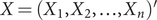
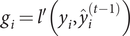
The average HFMD incidence is 38.84 per 100000 in the Xinjiang Autonomous Region from 2008 to 2018. Hereafter, all the following incidences are shown per 100000 population. The map in Figure 1 shows that the annual average HFMD incidence widely varied among different regions and is generated by the software ArcGIS 10.2 from http://eol.jsc.nasa.gov/ SearchPhotos/. The top two regions are Karamay and Urumqi, with incidence rates of 134.47 and 97.34, respectively. Hotan (0.50), Kashgar (0.67), Kizilsu (1.22), and Aksu (4.85) have relatively lower incidences.

Figure 1. The HFMD incidence in various regions of Xinjiang province.

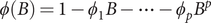
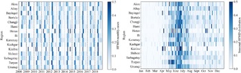
Based on the monthly reported data on HFMD cases, Figure 2 reflects the incidences of HFMD in 15 regions from 2008 to 2018. Further, the prevalence of HFMD has prominent seasonal characteristics in Xinjiang. It is concentrated between May and August, reaching 77.54% of the total cases.

Figure 2. The HFMD cases by the month of illness onset, standardized by the number of annual cases.

Analysis of meteorological factors

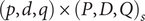
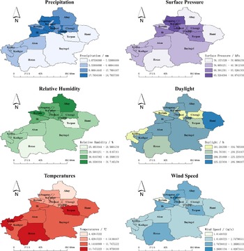
The monthly means ± standard error of the mean (SEM) of precipitation, temperature, sunshine hours, relative humidity, wind speed, and surface pressure of Xinjiang in 2008–2018 were (13.88 ± 16.13) mm, (10.33 ± 13.41)°C, (233.55 ± 80.83) h, (43.18 ± 16.01)%, (3.03 ± 0.73) m/s, and (89.73 ± 4.68) kPa, respectively. Figure 3 reflects each region’s monthly mean distribution of the above factors. We observe that there are regional variations of each meteorological factor. We use Moran’s $ I $ value to analyze the spatial autocorrelation of various meteorological factors in relation to HFMD incidence in Xinjiang from 2008 to 2018. The weight matrix of Moran’s $ I $ is generated by using the inverse distance weighting method. According to Table 1, Moran’s $ I $ values are all greater than 0. This indicates that the incidence of HFMD is spatially positively correlated in Xinjiang during the period 2008–2018. The $ p $ values are all less than 0.05 and statistically significant.

Figure 3. Monthly average values of meteorological indicators in Xinjiang regions.

Table 1. Spatial autocorrelation analysis of HFMD in Xinjiang from 2008 to 2018

The GTWR model is designed to analyze the influence of meteorological factors on HFMD transmission in time and space. The regression model is based on a weight matrix that integrates both temporal and spatial information [Reference Huang, Wu and Barry29]. Let $ X=\left({X}_1,{X}_2,\dots, {X}_n\right)^{\prime } $ , where $ {X}_i $ is the number of HFMD incidences in the $ i $ th region at time $ {t}_i $ , and let $ \left({u}_i,{v}_i\right) $ be the latitude and longitude coordinates of the $ i $ th region. The GTWR model is as follows:

(1) $$ {X}_i={\beta}_0\left({u}_i,{v}_i,{t}_i\right)+\sum \limits_{k=1}^p{\beta}_k\left({u}_i,{v}_i,{t}_i\right){C}_{ik}+{\varepsilon}_i,\hskip0.5em i=1,2,\dots, n, $$

where $ {C}_{ik} $ is the value of the $ k $ th meteorological variable in the $ i $ th region at time $ {t}_i $ , $ {\beta}_k\left({u}_i,{v}_i,{t}_i\right) $ is the corresponding weight, $ {\beta}_0 $ is the constant term and $ {\varepsilon}_i $ is the error term.

The coefficients $ {\beta}_k\left({u}_i,{v}_i,{t}_i\right) $ of meteorological factors can reflect the relationship between the HFMD incidence and meteorological variables. Through the weighted least square method and local linear geographical weighted regression, the estimates of the weight of the meteorological variables can be expressed as

(2) $$ \hat{\beta}\left({u}_i,{v}_i,{t}_i\right)={\left[{C}^T{W}_iC\right]}^{-1}{C}^T{W}_iX, $$

where $ {W}_i $ is the spatio-temporal weight matrix defined by spatio-temporal distance and bandwidth, and the elements in $ {W}_i $ are generated by

(3) $$ {\displaystyle \begin{array}{rcl}{w}_{ij}& =& \mathsf{\exp}\left\{-{\left(\frac{d_{ij}^{ST}}{h_{ST}}\right)}^2\right\}\\ {}& =& \mathsf{\exp}\left\{-\left(\frac{\lambda \left[{\left({u}_i-{u}_j\right)}^2+{\left({v}_i-{v}_j\right)}^2\right]+\mu {\left({t}_i-{t}_j\right)}^2}{h_{ST}^2}\right)\right\},\end{array}} $$

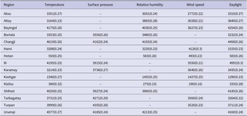
where $ {d}_{ij}^{ST} $ is the spatio-temporal distance between samples $ i $ and $ j $ , $ {h}^{ST} $ is the spatio-temporal bandwidth, $ \lambda $ , and $ \mu $ are scaling factors to determine the effects of spatial and temporal distances on the weights. After standardizing the HFMD data, Table 2 presents the average estimated values of the regression coefficients $ {\beta}_k\left({u}_i,{v}_i,{t}_i\right) $ .

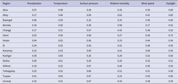
Table 2. The mean values of GTWR standardized coefficients of each meteorological variable

According to Table 2, the coefficients of precipitation are generally smaller than those of all factors. Therefore, this factor does not significantly affect the transmission of HFMD in each region. The effects of temperature and daylight are substantial in most regions. For different regions, other factors influencing the spread of HFMD vary significantly. For example, surface pressure is the most influential factor in Changji, Urumqi, and Tarbagatay, while it is insignificant in Hami and Hotan. Thus, these meteorological factors have significant spatial heterogeneity. The spread of HFMD transmission cannot be accurately described if meteorological factors are treated equally across all regions. Based on the above analysis, we conduct variable selection using the GTWR model. Then, the variables that have a significant impact on each region are incorporated into the prediction model.

SARIMA model

The SARIMA model can transform a non-stationary time series into stationary time ones. It is effective for studying time series with seasonal trends. To maintain the stationarity of the series, the trend and seasonality of HFMD incidence are eliminated using differencing [Reference Box, Jenkins, Reinsel and Ljung30]. Let $ {X}_t $ be the confirmed cases of HFMD at time $ t $ , and $ {\varepsilon}_t $ is the error term. A SARIMA model is defined as

(4) $$ {\displaystyle \begin{array}{r}\phi (B)\varPhi \left({B}^s\right){\left(1-{B}^s\right)}^D{\left(1-B\right)}^d{X}_t=\theta (B)\varTheta \left({B}^s\right){\varepsilon}_t,\end{array}} $$

where $ \phi (B)=1-{\phi}_1B-\cdots -{\phi}_p{B}^p $ and $ \theta (B)=1-{\theta}_1B-\cdots -{\theta}_q{B}^q, $ corresponding to the functions of the backshift operator $ B $ with $ {B}^l{X}_t={X}_{t-l} $ . Here, $ p $ is the autoregressive order, $ q $ is the moving average order, and $ d $ is the number of differencing operations. To eliminate seasonal variations, the SARIMA model uses seasonal differentials $ \left(1-{B}^s\right){X}_t $ , where $ s $ is the seasonal period of the data. The forms of $ \varPhi \left({B}^s\right) $ and $ \varTheta \left({B}^S\right) $ are as shown below:

$$ {\displaystyle \begin{array}{ccc}\varPhi ({B}^s)& =& 1-{\varPhi}_1{B}^s-\cdots -{\varPhi}_p{B}^{sP},\\ {}\Theta ({B}^s)& =& 1-{\Theta}_1{B}^s-\cdots -{\Theta}_Q{B}^{sQ},\end{array}} $$

where $ P $ is the seasonal autoregressive order, $ Q $ is the seasonal moving average order, and $ D $ is the number of seasonal differencing operations. We call (4) an SARIMA $ \left(p,d,q\right)\times {\left(P,D,Q\right)}_s $ model.

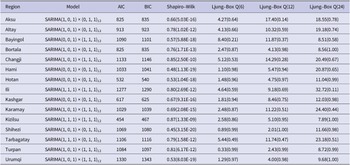
After removing the trend and seasonal components, the model fitting process includes order determination, parameter estimation, and diagnostic validation. The range of orders is determined by the autocorrelation function (ACF) and partial autocorrelation function (PACF). Within this range, multiple order combinations are traversed to obtain the optimal parameters that minimize the Akaike information criterion (AIC) and Bayesian information criterion (BIC) [Reference Burnham and Anderson31]. The parameters of the model are then estimated. In the diagnostic validation phase, the residuals are tested for normality and autocorrelation using the Shapiro–Wilk and Ljung–Box tests. The Shapiro–Wilk test, proposed by [Reference Shapiro and Wilk32], is a normality test as follows:

(5) $$ {\displaystyle \begin{array}{c}W=\frac{{\left({\varSigma}_{t=1}^N{a}_t{\varepsilon}_t\right)}^2}{\varSigma_{t=1}^N{\left({\varepsilon}_t-\overline{\varepsilon}\right)}^2},\end{array}} $$

where $ {\varepsilon}_t $ is the residual of the SARIMA model, $ \overline{\varepsilon} $ is the sample mean, and the coefficient $ {a}_t $ is the expected value of the standard normal statistic. Ljung–Box test [Reference Box and Pierce33, Reference Ljung and Box34] is expressed as

(6) $$ Q(m)=T\left(T+2\right)\sum \limits_{i=1}^m\frac{{\hat{\rho_i}}^2\left({\varepsilon}_t^2\right)}{T-i}, $$

where $ T $ is the sample size, i.e. the number of months included in the dataset, $ m $ is the maximum lagging order, $ {\varepsilon}_t $ is the residuals of the SARIMA model, and $ {\hat{\rho_i}}^2\left({\varepsilon}_t^2\right) $ is the $ i $ th order of the sample ACF. The Ljung–Box test reflects the autocorrelation of the series based on the autocorrelation coefficient of the series lagged at order $ k $ .

XGBoost algorithm

The XGBoost algorithm is an ensemble learning algorithm that incorporates a regularization term to control model complexity and avoid overfitting. Based on the classification and regression tree algorithm [Reference De’ath and Fabricius35], XGBoost is constructed by iteratively fitting the negative gradient values of the loss function to form a new model. As a result, it performs better in analyzing nonlinear data [Reference Ridgeway36]. Next, we review some basic concepts of the XGBoost algorithm [Reference Chen and Guestrin37]. Given $ n $ observations $ \left\{\left({\mathbf{x}}_i,{y}_i\right),i=1,2,\dots, n;{\mathbf{x}}_i\in {R}^d,{y}_i\in R\right\} $ , a tree ensemble model is established to predict the output where $ {f}_k $ is the kth decision tree, satisfying $ {f}_k\left(\mathbf{x}\right)={\omega}_{q\left(\mathbf{x}\right)} $ for $ \omega \in {R}^T $ and $ q:{R}^d\to T $ , $ T $ is the number of leaf nodes in the tree, and $ \omega $ is the weight vector of leaf nodes. The regularized objective function $ L\left(\phi \right) $ is composed of a loss function $ l\left({y}_i,{\hat{y}}_i\right) $ and a regular term $ \varOmega \left({f}_k\right) $ as follows:

$$ {\displaystyle \begin{array}{c}L\left(\phi \right)=\sum \limits_{i=1}^nl\left({y}_i,{\hat{y}}_i\right)+\sum \limits_{k=1}^K\varOmega \left({f}_k\right).\end{array}} $$

The second term $ \varOmega \left({f}_k\right) $ penalizes the complexity of regression three functions and is defined by 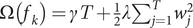$ \Omega \left({f}_k\right)=\gamma T+\frac{1}{2}\lambda {\sum}_{j=1}^T{w}_j^2 $ , where $ \gamma $ is the coefficient of the number of leaf nodes. Let $ {\hat{y}}_i^{(t)} $ be the prediction of the $ i $ th iteration. Since XGBoost uses the gradient-boosting decision tree pattern for the training set, it follows that 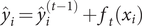$ {\hat{y}}_i={\hat{y}}_i^{\left(t-1\right)}+{f}_t\left({\boldsymbol{x}}_i\right) $ . Thus, we need to minimize the following objectives:

$$ {\displaystyle \begin{array}{c}{L}^{(t)}\left(\phi \right)=\sum \limits_{i=1}^nl\left({y}_i,{\hat{y}}_i^{\left(t-1\right)}+{f}_t\left({\boldsymbol{x}}_i\right)\right)+\varOmega \left({f}_t\right).\end{array}} $$

On the other hand, a second-order Taylor expansion at $ {\hat{y}}_i^{\left(t-1\right)} $ is derived from the loss function. Therefore, the loss function is rewritten as follows:

$$ l\left({y}_i,x\right)\approx {\displaystyle \begin{array}{l}l\left({y}_i,{\hat{y}}_i^{\left(t-1\right)}\right)+l^{\prime}\left({y}_i,{\hat{y}}_i^{\left(t-1\right)}\right)\left(x-{\hat{y}}_i^{\left(t-1\right)}\right)\\ {}+\hskip2px \frac{l^{{\prime\prime}}\left({y}_i,{\hat{y}}_i^{\left(t-1\right)}\right)}{2}{\left(x-{\hat{y}}_i^{\left(t-1\right)}\right)}^2.\end{array}} $$

Denote $ x={\hat{y}}_i^{\left(t-1\right)}+{f}_t\left({x}_i\right) $ , $ {g}_i=l^{\prime}\left({y}_i,{\hat{y}}_i^{\left(t-1\right)}\right) $ and $ {h}_i=l^{{\prime\prime}}\left({y}_i,{\hat{y}}_i^{\left(t-1\right)}\right) $ . The following objective can approximate the above objective function:

(7) $$ {\displaystyle \begin{array}{c}{L}^{(t)}\left(\phi \right)\approx \sum \limits_{i=1}^n\left[l\left({y}_i,{\hat{y}}_i^{\left(t-1\right)}\right)+{g}_i{f}_t\left({x}_i\right)+\frac{1}{2}{h}_i{f}_t^2\left({x}_i\right)\right]+\sum \limits_{k=1}^K\varOmega \left({f}_k\right).\end{array}} $$

The combined SARIMA-XGBoost model

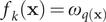
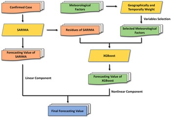
Through the analysis above, the SARIMA model can capture the historical patterns of HFMD prevalence well but cannot account for the endogenous factors affecting prevalence or capturing the complex factors of transmission due to its linear assumptions. To more accurately investigate the trend of HFMD cases, we introduce the XGBoost algorithm to effectively capture the nonlinear characteristics [Reference Zhang21]. We propose a combined SARIMA-XGBoost model to analyze both the linear and nonlinear components of the HFMD series. First, the SARIMA model is used to analyze the linear part of the series. Then, the residuals of the SARIMA model are considered the nonlinear part and are analyzed using the XGBoost model. Ignoring the effect of specific nonlinear factors can lead to poor performance in some situations. To address this, meteorological variables such as wind speed, relative humidity, and surface air pressure are included in the input layer of the XGBoost algorithm.

The flow chart of the SARIMA-XGBoost model is shown in Figure 4. Let $ {L}_t $ and $ {\hat{L}}_t $ be the true and fitting values from the SARIMA model (4) at time $ t $ , respectively. Suppose that the HFMD series is formed by the linear and nonlinear components:

$$ {\displaystyle \begin{array}{r}{X}_t={L}_t+{E}_t,\end{array}} $$

where $ {E}_t $ denotes the nonlinear part based on the XGBoost algorithm (7). The detailed process of the model is described as follows:

• (i) Through the SARIMA model (4), we obtain the corresponding residual values denoted by

  (8) $$ {\displaystyle \begin{array}{r}{e}_t={X}_t-{\hat{L}}_t.\end{array}} $$

• (ii) Analyze the meteorological factors for each region based on the GTWR model (1) and select the influential factors as meteorological variables denoted by $ {m}_1 $ , $ {m}_2 $ , $ \dots $ , $ {m}_n $ .

• (iii) Apply the XGBoost algorithm (7) to model the residuals (8). With n meteorological variables, the residual model is established as

  (9) $$ {\displaystyle \begin{array}{r}{e}_t=f\left({m}_1,{m}_2,\dots, {m}_n\right)+{\varepsilon}_t,\end{array}} $$

Figure 4. The flow chart of the combined SARIMA-XGBoost model.

where $ f $ is a nonlinear function determined by the XGBoost algorithm, and $ {\varepsilon}_t $ is the random error. Let $ {\hat{E}}_t $ be the estimated values of $ {e}_t $ . The estimator $ {\hat{X}}_t $ of $ {X}_t $ is

$$ {\displaystyle \begin{array}{r}{\hat{X}}_t={\hat{L}}_t+{\hat{E}}_t.\end{array}} $$

To ensure a comprehensive and balanced evaluation, we employ four indexes to assess the performance of the combined SARIMA-XGBoost model: the root mean square error (RMSE), coefficient of determination ( $ {R}^2 $ ), mean absolute error (MAE), and symmetric mean absolute percentage error (SMAPE). RMSE offers insights into the forecast’s accuracy by quantifying the average discrepancies between the actual and predicted values. $ {R}^2 $ , a measure of the model’s goodness of fit, indicates the percentage of variance in the dependent variable accounted for by the independent variables. MAE measures the mean magnitude of errors by averaging the absolute differences between observed and predicted values. In addition, SMAPE provides a relative error measurement, factoring in symmetric penalties for both overpredictions and underpredictions. The model’s accuracy is considered higher as $ {R}^2 $ approaches 1 and as RMSE, MAE, and SMAPE values decrease. The formulas to compute these metrics are as follows:

$$ {\displaystyle \begin{array}{r}\begin{array}{c}\mathrm{R}\mathrm{M}\mathrm{S}\mathrm{E}=\sqrt{\frac{1}{M}\sum \limits_{t=1}^M{({X}_t-{\hat{X}}_i)}^2},\\ {}\hskip1em {R}^2=1-\frac{\sum \limits_{i=1}^M{({X}_i-{\hat{X}}_i)}^2}{\sum \limits_{i=1}^M{({X}_i-{\overline{X}}_i)}^2},\\ {}\mathrm{M}\mathrm{A}\mathrm{E}=\frac{1}{M}\sum \limits_{i=1}^M|{\hat{X}}_i-{X}_i|,\\ {}\mathrm{S}\mathrm{M}\mathrm{A}\mathrm{P}\mathrm{E}=\frac{100\%}{M}\sum \limits_{i=1}^M\frac{|{X}_i-{\hat{X}}_i|}{(|{X}_i|+|{\hat{X}}_i|)/2},\end{array}\hskip2.00em \end{array}} $$

where $ {X}_i $ is the actual observed value, $ {\overline{X}}_i $ is the mean value of $ {X}_i $ , $ {\hat{X}}_i $ is the predicted value, and $ M $ denotes the number of samples.

Analysis of SARIMA-XGBoost model

In the SARIMA-XGBoost model, we first establish the SARIMA model determined by the following steps:

• • Apply the augmented Dickey–Fuller test to determine the stationarity of the HFMD incidence series in 15 regions of Xinjiang from 2008 to 2018. If the series is non-stationary, use differencing to transform it into a stationary series.

• • Determine six parameters $ p $ , $ d $ , $ q $ , $ P $ , $ D $ , and $ Q $ according to the ACF and PACF plots.

• • Based on the AIC and BIC criteria, conduct multiple order combinations to determine the optimal parameters.

The model residuals are analyzed through the Shapiro–Wilk and Ljung–Box tests to determine the effectiveness of the SARIMA model. The diagnosis of the model and the test results are shown in Table 3. All the $ p $ values exceed the significance level of 0.05, indicating that the residual series pass the Ljung–Box test. This suggests that the SARIMA model successfully captures the temporal autocorrelation in the HFMD incidence data. However, all $ p $ values of the Shapiro–Wilk test are less than 0.05, the residual series do not pass the normality test. This may indicate that the SARIMA model has not adequately captured the structure of the data, and there could be nonlinear trends present. Using the SARIMA model alone is less effective for analyzing HFMD trends in each region.

Table 3. Diagnosis of SARIMA (p, d, q) × (P, D, Q) _s model

To capture the nonlinear characteristics in the residuals, based on the SARIMA (p, d, q) × (P, D, Q) _s model listed in Table 3, meteorological variables corresponding to each region serve as input for the XGBoost algorithm, as introduced in equation (7). During the training of the XGBoost algorithm, the choice of parameters significantly affects the model’s effectiveness. Thus, parameters like the maximum number of iterations, maximum tree depth, and random sampling ratio are carefully considered. For instance, in Urumqi, the chosen parameters are a maximum of 4000 iterations, a maximum tree depth of 6, a learning rate of 0.1, and a random sampling ratio of 0.5. Details on the parameter-tuning process will follow:

• • Considering the different factors, we first normalize the meteorological data. Based on the standardized regression coefficient (Table 2) of the GTWR model, the four important factors are selected as input variables of the XGBoost algorithm for each region.

• • Determine the ‘booster’ to be ‘gbtree’; that is, the tree model is regarded as the base model. The objective parameter is selected as ‘reg:squarederror’, corresponding to a regression problem with minimizing MSE.

• • Take the learning rate to be 0.1, and then use the built-in ‘xgb.csv’ function. The ‘xgb.csv’ function will return the optimal maximum number of iterations.

• • For the remaining parameters, the range of parameters is first determined, and then the ‘GridSearchCV’ function is used to traverse and search the optimal parameters.

In the implementation of the XGBoost algorithm, a tree model is used as the base model. Within this tree model, input variables serve as split nodes and are associated with different gain values of the objective function. A higher gain value indicates a greater influence of the variable on the model. Therefore, the importance of each variable can be assessed by the frequency with which it is used as a split node. Table 4 presents the feature importance of the meteorological variables, measured by their use as split nodes during the training of the XGBoost algorithm. This provides insights into the impact of the selected meteorological factors on the incidence of HFMD in each region.

Table 4. The feature important and percentage of meteorological variables for each region

Compared with other models

In this section, we compare the performance of the SARIMA-XGBoost model to other models, such as SARIMA, XGBoost, long-/short-term memory (LSTM) networks, and support vector regression (SVR) models. The process for establishing the SARIMA-XGBoost model is described in the Section ‘The SARIMA-XGBoost model’. To provide effective information for the rational allocation of medical resources across various regions, we use a dataset comprising the number of HFMD patients in 15 regions of Xinjiang from 2008 to 2018. The first nine years of data serve as the training set, while the data from 2017 to 2018 is used as the test set. The regional incidence can also be predicted by dividing the number of patients by the total number of people in the area, which will help eliminate the effect of differences in population density and make comparisons between different regions fairer.

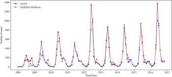
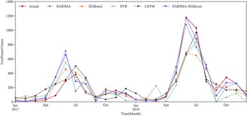
We use the prediction results for Urumqi as an example. Based on the critical meteorological factors outlined in Table 4, Figures 5 and 6 show the fitting result graph for the training set and the comparison of prediction in Urumqi. When comparing with other models, we individually optimize each model to ensure predictive accuracy. For example, given the XGBoost model’s strength in ensemble learning, we incorporate meteorological variables into its predictions. Numerical simulations show that the predictive accuracy of the LSTM model decreases when incorporating meteorological factors as input variables. Consequently, we use just the historical HFMD cases as the input feature for the LSTM model. It can be observed that the SARIMA-XGBoost model outperforms the other models. Specifically, the RMSE values for SARIMA, XGBoost, LSTM, and SVR are 147.51, 152.75, 129.43, and 167.01, respectively. The proposed SARIMA-XGBoost model has an RMSE of 112.51, which is significantly lower than those of the other models. The $ {R}^2 $ value for the SARIMA-XGBoost model is higher by 13.3%, 16.4%, 7.5%, and 25% when compared to SARIMA, XGBoost, LSTM, and SVR, respectively. Additionally, the SARIMA-XGBoost model exhibits the lowest values among the five models for both MAE and SMAPE metrics.

Figure 5. The fitting result graph for the training set in Urumqi.

Figure 6. The prediction results of Urumqi in five models.

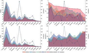
Figure 7 presents the RMSE, $ {R}^2 $ , MAE, and SMAPE values of five models used for predicting the 15 regions in Xinjiang during 2017–2018. Considering the above four metrics, the SARIMA-XGBoost model significantly outperforms other models in prediction. For example, the $ {R}^2 $ of the SARIMA-XGBoost model increases by 58.5%, 38.3%, 54%, and 111%, compared to the SARIMA model, XGBoost algorithm, LSTM, and SVR model, respectively. In regions with higher incidence, such as Changji, Urumqi, Bortala, Tarbagatay, and Karamay, the SARIMA-XGBoost model demonstrates minor deviations and greater robustness than other models, with a notable improvement in accuracy. However, for regions with lower incidence like Kizilsu, Kashgar, and Hotan, the prediction accuracy of the SARIMA-XGBoost model is comparatively lower. One of the primary reasons is that both SARIMA models and machine learning methods demand ample data to achieve accurate predictions, which is lacking in these regions with lower incidence. For instance, over the past decade in Hotan, around 73.5% of the months reported zero cases, and approximately 93.2% of the months reported fewer than five cases. This limited data poses challenges for precise predictions. Moreover, the differences and fluctuations of meteorological factors in regions with low incidence are not as pronounced. Despite these challenges, the SARIMA-XGBoost model still significantly enhances RMSE, $ {R}^2 $ , MAE, and SMAPE values compared with other models.

Figure 7. Evaluation results of different models for the prediction of 15 regions in Xinjiang.

Based on the above analysis, we can conclude that the proposed SARIMA-XGBoost model can achieve better performance in predicting HFMD.