2.1. Stratified shear layer

The problem of a temporally evolving stratified shear layer with uniform stratification is considered. A sketch of the shear layer with relevant initialization parameters is shown in figure 1. The flow is constructed with a streamwise velocity field given by

(2.1)\begin{equation} \langle u^* \rangle(z^*,t=0) ={-}\frac{{\Delta} U^*}{2} \tanh\left( \frac{2 z^*}{\delta^*_{\omega,0}}\right) , \end{equation}

where $\Delta U^*$ denotes the velocity difference across the shear layer and $\delta ^*_{\omega ,0} = \Delta U^*/(\mathrm {d}\langle u^*\rangle /\mathrm {d}z^*)_{{max}}$ is the initial vorticity thickness. Note that a superscript $*$ denotes a dimensional quantity while the $\langle \cdot \rangle$ operator indicates horizontal averaging.

Figure 1. Sketch of the stratified shear layer with constant stratification.

Motivated by atmospheric and ocean observations in which stratification extends beyond regions of shear (Fritts Reference Fritts1982; Smyth, Moum & Caldwell Reference Smyth, Moum and Caldwell2001), this work utilizes a spatially extensive stratification. The density profile is initialized by a time-invariant uniformly stratified background density profile ($\rho _b^*$). The background buoyancy frequency of the ambient fluid (${N_0^*}^2$) has a constant value given by ${N_0^*}^2=-(g^*/\rho ^*_0)\, \mathrm {d}\rho _b^*/\mathrm {d}z^*$, where $g^*$ is gravity and $\rho ^*_0$ is a reference density.

The governing equations for this problem are the three-dimensional Navier–Stokes equations for an unsteady, incompressible flow with the Boussinesq approximation. A Cartesian frame of reference is used to represent the streamwise, spanwise and vertical coordinates such that spatial orientation and velocities are given by $x_i=(x,y,z)$ and $u_i=(u,v,w)$, respectively. The density equation is solved for the non-dimensional density deviation ($\tilde {\rho }$) from the uniform background. Similarly, the pressure ($p$), which denotes the deviation from the pressure which is in hydrostatic balance with the background density ($\rho _b^*$), is solved for. The governing equations are non-dimensionalized using the following reference quantities: velocity difference ($\Delta U^*$), initial vorticity thickness ($\delta ^*_{\omega ,0}$) and a reference value for density deviation ($\Delta \rho ^*=\delta ^*_{\omega ,0}\,\mathrm {d}\rho _b^*/\mathrm {d}z^*$). The resulting non-dimensional equations are given by

(2.2a)\begin{gather} \frac{\partial u_j}{\partial x_j} = 0 , \end{gather}

(2.2b)\begin{gather}\frac{\partial u_i}{\partial t} + \frac{\partial (u_ju_i)}{\partial x_j} ={-}\frac{\partial p}{\partial x_i} +\frac{1}{Re}\frac{\partial^2 u_i}{\partial x_j \partial x_j} - Ri\tilde{\rho} g_i , \end{gather}

(2.2c)\begin{gather}\frac{\partial \tilde{\rho}}{\partial t} + \frac{\partial (u_j \tilde{\rho})}{\partial x_j} = \frac{1}{Re\, Pr}\frac{\partial^2 \tilde{\rho}}{\partial x_j \partial x_j} - w . \end{gather}

Non-dimensional parameters, namely the initial Reynolds number ($Re$), initial gradient Richardson number at the centre of the shear layer ($Ri$) and Prandtl number ($Pr$) are as follows:

(2.3a–c)\begin{equation} Re = \frac{\Delta U^* \delta^*_{\omega,0}}{\nu^*} , \quad Ri = \frac{N^{*2}_0 \delta^{*2}_{\omega,0}}{\Delta U^{*2}} , \quad Pr = \frac{\nu^*}{\kappa^*} . \end{equation}

Here, $\nu ^*$ and $\kappa ^*$ are the kinematic viscosity and thermal diffusivity, respectively.

2.2. Numerical methods and simulation set-up

Five DNS cases are simulated as listed in table 1. All cases have $Re=24\,000$ and $Pr=1$ while the strength of stratification is varied such that $Ri=[0.04, 0.08, 0.12, 0.16, 0.2]$ encompasses a wide range of background stability from weakly stratified at $Ri=0.04$ to strongly stratified at $Ri=0.2$.

Table 1. Parameters used to construct the computational domain: domain length ($L_x, L_y, L_z$), region with uniform grid spacing in the vertical direction ($L_{z,sl}$), number of grid points ($N_x, N_y, N_z$), grid spacing in the shear layer ($\varDelta$), grid spacing normalized by the smallest Kolmogorov length scale and peak wavenumber $k_0$ of the energy spectrum used to generate the initial velocity perturbations. The thickness of the upper TL ($\delta _{TL}$) at late time is given in the last column.

The numerical methods employed to solve the governing equations are similar to DNS of our previous work (Brucker & Sarkar Reference Brucker and Sarkar2007; Pham & Sarkar Reference Pham and Sarkar2010; VanDine, Chongsiripinyo & Sarkar Reference VanDine, Chongsiripinyo and Sarkar2018). The Williamson low-storage, third-order Runge–Kutta method is employed for time advancement while the discretization of spatial derivatives is achieved using a second-order, central finite difference scheme. The Poisson equation for pressure is solved using a parallel multigrid solver. The streamwise and spanwise directions have periodic boundary conditions. In the vertical direction, vertical velocity has a homogeneous Dirichlet boundary condition while homogeneous Neumann boundary conditions are enforced for horizontal velocity components, density deviation and pressure. In a sponge region near the vertical boundaries in the regions $z>10$ and $z<10$ (sufficiently far from the shear layer), a Rayleigh damping function gradually relaxes the density and velocities to their corresponding boundary values in order to damp propagating fluctuations and prevent reflections of features such as internal waves which have propagated far from the shear layer.

For this work, an isotropic grid is used in the central region of the shear layer with a grid spacing of $\Delta x=\Delta y=\Delta z=\varDelta$ as indicated in table 1. The streamwise and spanwise grids have uniform spacing while mild stretching is used in the vertical outside the shear layer. Throughout the entire grid, the grid spacing is less than $2.2\eta$, where $\eta =(\nu ^3/\varepsilon )^{1/4}$ ($\varepsilon$ denotes turbulent kinetic energy dissipation rate) is the Kolmogorov length scale, thus indicating appropriate resolution for capturing small-scale fluctuations. The number of grid points in the streamwise, spanwise and vertical directions are given by $(N_x,N_y,N_z)$ and the domain extent is given by $(L_x,L_y,L_z)$ as denoted in table 1. The computational domain is large enough to accommodate two wavelengths of the most unstable Kelvin–Helmholtz (K–H) mode in the streamwise direction and one wavelength in the spanwise direction. The sufficiently large spanwise domain is required in order to accurately capture the transition from two-dimensional K–H shear instability to three-dimensional turbulence and also to ensure good convergence of statistics. The spanwise domain size is about two times and the number of grid points is about four times larger than in the cases of Mashayek, Caulfield & Peltier (Reference Mashayek, Caulfield and Peltier2013) with the equivalent $Re$. Due to the different characteristic length and velocity scales used in the non-dimensionalization of the governing equations, the Reynolds number of 24 000 in the present study is equivalent to $Re = 6000$ in Mashayek & Peltier (Reference Mashayek and Peltier2013). We choose this value of $Re$ since their results suggest the influence of secondary instabilities on the rate of mixing is most profound when Re is at or larger than this value.

The flow is initialized using velocity perturbations for which the broadband spectrum is given by $E(k) \propto k^4 \exp [ -2 ( k/k_0 )^2]$, where the peak value of $E(k)$ is found at $k_0$ (values given in table 1) corresponding to the fastest growing mode of the K–H instability. The root mean square (r.m.s.) of each velocity component has a peak of 0.1 % $\Delta U$ at the centre of the shear layer. The following shape function, $F(z) = \exp [-( z/\delta _{\omega ,0} )^2]$, is used to confine the fluctuations to inside the shear layer.

2.3. Linear stability analysis of K–H shear instability

In order to construct the computational grid, linear stability analysis (LSA) is performed to search for the fastest growing normal mode of the K–H shear instability. Stability theory of a stratified shear layer with a two-layer hyperbolic density profile suggests a condition of $Ri < 0.25$ for the shear instability to develop. The growth rate ($\sigma$) of the fastest growing mode (FGM) is significantly reduced as $Ri$ increases toward 0.25 in an analysis (Hazel Reference Hazel1972) which assumes that the fluid is inviscid and that the shear layer is located inside an infinite domain.

Here, the LSA is performed, taking into account the effect of viscosity, diffusivity and a finite domain, to examine the FGM when the shear layer is uniformly stratified. The theory and numerical implementation of the LSA is given in Smyth, Moum & Nash (Reference Smyth, Moum and Nash2011). In the LSA, the Reynolds number, Prandtl number and domain size ($L_z$) have the same values as in the DNS. The grid spacing is $\Delta z=0.025$. Free-slip and fixed buoyancy conditions are used at the top and bottom boundaries. The LSA of the two-layer profile is also performed for comparison.

Figure 2(a,b) contrasts the mean profiles of the squared buoyancy frequency ($N^2$), squared rate of shear ($S^2$) and gradient Richardson number ($Ri_g$) in the two-layer shear layer to those in the linearly stratified shear layer. The same level of stratification at the centre of the shear layer, $N^2 = 0.12$, is used. Away from the centre, $N^2$ decreases to zero in the two-layer case while it remains constant in the other case. As a result, $Ri_g$ in the two-layer case is smaller than that in the case with linear stratification throughout the shear layer except at the centre where $Ri_g = 0.12$ in both cases. With the same amount of mean kinetic energy, e.g. the same velocity profile, the potential energy barrier inside the shear layer is significantly higher in the case with linear stratification, thereby reducing the growth rate of the K–H shear instability.

Figure 2. Effect of stratification on flow instability using LSA. Plots (a,c,e) correspond to the two-layer density profile and (b,d,f) to the linear density profile with uniform $N^2$. (a,b) Initial profiles of $S^2$, $N^2$ and $Ri_g$. (c,d) Contours of growth rate ($\sigma$) as a function of $Ri$ and wavenumber ($k$). (e,f) Plots showing $\sigma$($k$) in the five simulated $Ri$ cases. Dashed magenta lines in (c,d) mark the stability boundary, $Ri = k(1/2-k/4)$ (Hazel Reference Hazel1972) and $Ri = k^2(1/4-k^2/16)$ (Drazin Reference Drazin1958), respectively. Solid white lines in (c,d) indicate the location of the FGMs of the K–H instability.

Results of the LSA are shown in figure 2(c,d). In the two-layer case, the growth rate ($\sigma$) is similar to that of Hazel (Reference Hazel1972) in the region with low $k$ and $Ri$. However, as $k$ and $Ri$ increase, the growth rate becomes slightly smaller than the value from Hazel (Reference Hazel1972) due to the effect of viscosity, diffusivity and a finite domain. The location of FGMs (marked by a white line) in $k\delta _{\omega ,0} - Ri$ space indicates a significant difference between the two configurations. While the wavenumber of the K–H modes varies little with $Ri$ in the two-layer case, the K–H modes show a larger value of $k$ and thus a shorter wavelength as $Ri$ increases in the case with uniform stratification. Figure 2(e,f) contrasts the growth rate between the two cases for the five values of $Ri$ used in the DNS to be discussed. At the same $Ri$, the growth rate of the K–H mode is higher in the two-layer case which suggests the K–H shear instability in the case with uniform stratification is weaker.

2.4. Statistical analysis

The velocity, density and pressure fields are decomposed using Reynolds decomposition into mean (horizontal average) and fluctuating components denoted by $\langle \rangle$ and $'$, respectively. In later discussions, the turbulent kinetic energy (TKE) budget will be used to examine the routes to turbulence and is given by

(2.4)\begin{equation} \frac{\mathrm{D} K}{\mathrm{D} t} = {P} - \varepsilon + {B} - \frac{{\partial} {T}_3}{{\partial} z} , \end{equation}

with TKE (${K}$), production (${P}$), dissipation ($\varepsilon$), buoyancy flux (${B}$) and the transport term (${T}_3$) specified as

(2.5) \begin{equation} \left.\begin{gathered} {K} = \frac{1}{2} \left( \langle u'\rangle^2 + \langle v'\rangle^2 + \langle w'\rangle^2\right), \\ P = -\langle u'w' \rangle \frac{\partial \langle u \rangle}{\partial z}, \quad \varepsilon = \frac{2}{Re} \langle s_{ij}' s_{ij}' \rangle, \quad s_{ij}' = \frac{1}{2} \left( \frac{\partial u_i'}{\partial x_j} + \frac{\partial u_j'}{\partial x_i} \right), \\ {B} ={-}Ri \langle \rho' w' \rangle, \quad {T}_3 = \frac{1}{2} \langle w' u_i' u_i' \rangle + \frac{1}{\rho_0} \langle w'p' \rangle - \frac{2}{Re} \langle u_i' s_{3i}' \rangle. \end{gathered}\right\} \end{equation}

In order to calculate mixing efficiency, numerous studies have used a method which quantifies available and background potential energy by sorting the density field (Winters et al. Reference Winters, Lombard, Riley and D'Asaro1995). This method produces a bulk value of the mixing efficiency which is representative of the entire shear layer. Instead, we use the dissipation of the density field as a surrogate to the change in background potential energy such that the mixing efficiency ($E$) is given by

(2.6a,b)\begin{equation} {E} =\frac{\varepsilon_\rho}{\varepsilon+\varepsilon_\rho} , \quad \varepsilon_\rho=\frac{1}{Re\, Pr} \frac{g^2}{\rho_0^2 N^2_0} \left \langle \frac{\partial \rho'}{\partial x_i} \frac{\partial \rho'}{\partial x_i} \right\rangle , \end{equation}

where $\varepsilon _\rho$ is the dissipation rate of turbulent available potential energy ($\textrm {TAPE} = g^2\left \langle \rho '^2\right \rangle /2\rho _0^2N_0^2$). Scotti & White (Reference Scotti and White2014) have demonstrated that this method of computing the mixing efficiency produces accurate results for turbulence in a continuously stratified fluid. Furthermore, this method is able to provide the spatial variability of the mixing efficiency throughout the shear layer as opposed to a single bulk value.

3.1. Routes to turbulence: K–H shear instability and secondary instabilities

In a shear layer with inflectional shear it is understood that there is a strong primary instability in the form of a K–H shear instability. This instability manifests as a series of vortices which roll up over time (termed billows) and are connected by vorticity filaments (termed braids). As the K–H billows evolve, secondary instabilities develop throughout the shear layer (Mashayek & Peltier Reference Mashayek and Peltier2012a,b; Thorpe Reference Thorpe2012; Arratia, Caulfield & Chomaz Reference Arratia, Caulfield and Chomaz2013; Salehipour et al. Reference Salehipour, Peltier and Mashayek2015). In the following discussion we use the visualization of density and vorticity fields to illustrate that, as in the shear layer between two layers of constant density, the continuously stratified shear layer exhibits rich dynamics of secondary instabilities. In the present study we do not perform LSA for each type of instability since they are already discussed in depth in previous studies. Instead, we focus on the effect of the continuous stratification and the resulting mixing driven by the secondary instabilities. Our identification of secondary instabilities is based on visual inspection and comparison with previous work in the two-layer problem. It is also noted that pairing of K–H billows is not found at the high $Re$ of the present study. At sufficiently high $Re$, secondary instabilities break down the billows before their co-rotation and pairing as was found by Pham & Sarkar (Reference Pham and Sarkar2010) when $Re$ was increased to 5000 relative to their earlier work at $Re = 1280$.

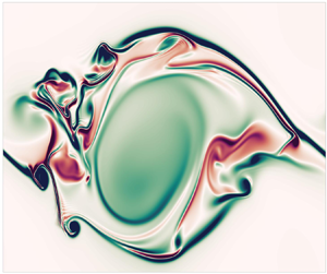
The $Ri=0.04$ case is used to outline the general development of the stratified shear layer, and differences between the various $Ri$ cases are discussed thereafter. Figure 3 shows cross-sectional snapshots of the density ($\rho$) and spanwise vorticity ($\omega _2=\partial u/\partial z - \partial w/\partial x$). Specific snapshots in time are shown where the time ($t$) represents the non-dimensional time, $S_0^* t^*$, where $S_0^*$ is the initial centreline shear. The primary shear instability is evident in figure 3(a) in the form of two K–H billows. As the billows grow vertically, they extract kinetic energy from the shear layer. Once they reach the maximum vertical extent, the K–H billows spread in the streamwise direction and deform into elliptical shape similar to the observation by Arratia (Reference Arratia2011). A spanwise variability also develops early to further disrupt the flow as indicated in the spanwise snapshots of $\rho$ and $\omega$ in figure 3(a). The billow continues to develop horizontal motions and r.m.s. spanwise velocity fluctuations (not shown) increase in this case. Note that there is no broadband turbulence as yet in the development. As small-scale fluctuations are allowed to develop due to low viscosity (high $Re$), the billows begin to break down by secondary instabilities. A counter-rotating vortex pair denoting secondary convective instability (SCI) is seen at $(x,z)\approx (7,0)$ in the streamwise snapshot of $\omega _2$ in figure 3(b). Multiple occurrences of SCI develop in the eyelids of the two billows. The spanwise snapshot of $\omega _2$ suggests the SCI is highly three dimensional unlike the two-dimensional K–H billows with little spanwise variability seen at the earlier time. Strong vortices which develop in the centre of the billow cores at $(x,z)\approx (3,0)$ and (8,0) also contribute towards transition to turbulence. In the DNS with uniform stratification at $Re = 10\,000$ and $Ri = 0.05$, Fritts et al. (Reference Fritts, Baumgarten, Werne and Lund2014) observed that secondary instabilities arise initially in the eyelid and the resulting turbulence spreads inward into the core. Here, we observe growth of SCI in the eyelids and strong vortices in the billow cores at the same time. Eventually, the breaking billows become localized patches of turbulence with the majority of overturning occurring at the core of each billow as shown in figure 3(c).

Figure 3. Cross-sectional snapshots of the density ($\rho$) and spanwise vorticity ($\omega _2$) fields for the $Ri=0.04$ case at (a) $t = 59$, (b) $t = 83$ and (c) $t = 86$. From left to right, the columns show a streamwise cross-section of $\rho$ at $y = L_y/2$, spanwise cross-section of $\rho$ along the dotted line shown in the first column, streamwise cross-section of $\omega _2$ at $y = L_y/2$ and a spanwise cross-section of $\omega _2$ along the dotted line shown in the third column. In this plot and henceforth, $x$, $y$ and $z$ are noted to be the streamwise, spanwise and vertical coordinates, respectively, made non-dimensional using $\delta _{\omega ,0}$.

The flow evolves differently at moderate stratification ($0.08 \leqslant Ri \leqslant 0.16$) with the K–H billows exhibiting smaller vertical growth followed by faster spreading in the streamwise direction and deformation into elliptical billows as illustrated in figure 4. Unlike the $Ri = 0.04$ case in which the SCI initiates the transition to three-dimensional turbulence, the streamwise snapshots of $\rho$ and $\omega _2$ in figure 4(a) indicates the secondary shear instability (SSI) also contributes to the transition. The negative-$\omega _2$ vortices which grow along the braids in the regions $1 < x < 2$ and $9.5 < x < 10.5$ are indicative of SSI. As $Ri$ increases, SSI overtakes SCI as the dominant mechanism that breaks down the K–H billows when contrasting figures 4(a) through 4(c). In $Ri = 0.08\text {--}0.16$ cases, vortices that grow at the top of the left billow are suggestive of secondary core deformation instability (SCDI). Mashayek & Peltier (Reference Mashayek and Peltier2012b) found SCDI is associated with an observable inflation of the core. They also suggested that the growth rate of SCDI decreases with increasing $Ri$. The vortices that break down the left billow in figure 4(a–c) are also less energetic as $Ri$ increases.

Figure 4. Cross-sectional snapshots of the density ($\rho$) and spanwise vorticity ($\omega _2$) fields for the four cases with $Ri \geqslant 0.08$. The column order is similar to figure 3: streamwise and spanwise cross-sections of $\rho$ followed by streamwise and spanwise cross-sections of $\omega _2$. Note that the panels have differing aspect ratios and cover different ranges of $x$ and $z$ coordinates.

Beside SCI, SSI and SCDI, we also observe the development of localized core vortex instability (LCVI). When the core vortex bands grow and achieve a sufficiently large magnitude of $\omega _2$, LCVIs form at the tips of the vorticity bands. The LCVI vortices and the bands from which they develop have spanwise vorticity with sign opposite to the background shear-layer vorticity (Mashayek & Peltier Reference Mashayek and Peltier2012b). The appearance of LCVI is particularly apparent at high $Re$ because the K–H billows roll-up faster and there is less time for the vorticity bands in the core to diffuse. The streamwise snapshot of $\omega _2$ shows positive (red) vortices at $(x,z)\approx (6,0)$ and $(7,0)$ in figure 4(a). The two vortices develop from the tips of the negative (green) vortex bands in the eyelid indicating the growth of a LCVI.

At the high stratification of the $Ri = 0.2$ case, the transition to turbulence is induced by SCDI and SCI. The multiple coherent vortices which develop in the lower half of the billow at $(x,z)\approx (6,-0.5)$ in the streamwise snapshots of figure 4(d) are indicative of SCDI. The vertical strips of positive density at $y = 2$ and negative density at $y = 4.2$ in the spanwise snaphot are indicative of SCI. The strips resemble mushroom-like structures, a typical morphology of convective instabilities. We note the use of a large aspect ratio in figure 4(d) which distorts the mushroom-like structures into the vertical strips. While the mushroom-like structures in the $Ri = 0.04$ case develop on the thin eyelid region of the K–H billows, the structures in this case with $Ri = 0.2$ are significantly larger and they penetrate across the entire vertical extent of the billow. The DNS of Fritts et al. (Reference Fritts, Baumgarten, Werne and Lund2014) at the same $Ri$ but with $Re = 10\,000$ shows the prevalence of secondary instabilities in the billow cores. The absence of SCDI in their study is possibly due to a low Reynolds number effect.

There are multiple modes that have similar vorticity manifestation such as the stagnation point instability (SPI) and secondary vortex band instability (SVBI). In fact, Mashayek & Peltier (Reference Mashayek and Peltier2013) found that SVBI is a combination of both SPI and LCVI. Therefore, it is difficult to differentiate LCVI from SVBI without performing the stability analysis. Furthermore, the growth of secondary instabilities is highly sensitive to the initial broadband velocity fluctuations (Dong et al. Reference Dong, Tedford, Rahmani and Lawrence2019). We have simulated the $Ri = 0.16$ case with two different choices for the initial velocity perturbations: one where the energy spectrum peaks at $k_0 = 1.13$ and another with a peak at $k_0 = 1.24$. The horizontal domain length is chosen to accommodate two wavelengths of the most energetic mode in the initial velocity perturbations. While the evolution of the shear layer is statistically similar between the two cases, we find SPI to develop in only the former simulation with $k_0 = 1.13$ and not the latter. The SPI manifests as a single vortex which develops at the stagnation point in the braid. Overall, with regard to the secondary instabilities, the transition to turbulence in the shear layer with uniform stratification is as dynamically rich as that observed in the case with a two-layer density profile. Readers should be aware that there are other secondary instabilities that have not been observed in either Mashayek & Peltier (Reference Mashayek and Peltier2013) or the present study such as knot and tube instabilities (Thorpe Reference Thorpe2012).

3.2. Effect of stratification on the growth of shear-layer thickness

The visualization of the evolving shear layer suggests that the thickness of the shear layer varies significantly with the stratification. Here, we quantify the thickness of the shear layer through two quantities: (1) the momentum thickness ($I_u$) and (2) the layer bounded by the outer edges of the TLs denoted by $L_{sl}$. The first quantity provides an integral length scale which is used to compute non-dimensional numbers such as the bulk Richardson number, an important parameter typically used in the parameterization of shear-driven turbulence (Smyth & Moum Reference Smyth and Moum2000; Mashayek, Caulfield & Peltier Reference Mashayek, Caulfield and Peltier2017a). In contrast, the second quantity includes the mixing region at the edges of the shear layer. In the present study we identify the TL as a region with enhanced stratification (i.e. $N^2/N_0^2 > 1$) formed at the edge of the shear layer due to vertical turbulent transport from the core of the shear layer to its edge. Figure 5 indicates a significant difference between the two quantities with $L_{sl}$ up to 60 % larger than $I_u$ in the $Ri = 0.16$ case at late time. In this section we focus the discussion on $I_u$ and defer consideration of $L_{sl}$ to the next section.

Figure 5. Temporal evolution of (a) momentum thickness ($I_u$) and (b) shear-layer thickness ($L_{sl}$) defined by the outer edges of the TL.

The momentum thickness, which is defined as

(3.1)\begin{equation} I_u=\int_{{-}10}^{10} \left[1-4\left\langle u\right\rangle^2\right] \mathrm{d}z \end{equation}

has the imprint of distinct flow regimes. At early time (approximately $30 < t < 60$ in the $Ri=0.04$ and $Ri=0.08$ cases, and $50< t<90$ in the $Ri=0.12$ case), the shear layer thickens rapidly due to the enlargement of the K–H billows. In all cases, except for the $Ri \geqslant 0.16$ cases, there is a period where the shear layer briefly shrinks or stops growing before resuming its growth (approximately $60< t<80$ in the $Ri=0.04$ and $Ri=0.08$ cases, and $100< t<110$ in the $Ri=0.12$ case). At $Ri = 0.12$, the layer does not contract significantly as in the $Ri=0.04$ and $Ri=0.08$ cases but its growth pauses. The contraction of the shear layer persists longer at smaller $Ri$ and is not seen at all in the $Ri \geqslant 0.16$ cases indicating a key link of stratification to this flow feature. The period of contraction occurs during the transition from flow dominated by two-dimensional K–H rollers to fully three-dimensional turbulence. After its contraction or pause, $I_u$ resumes growing before it asymptotes to a constant value at late time. At this time, buoyancy effects become sufficiently strong to cause turbulence decay and the shear layer can no longer thicken. Overall, the rate of growth decreases with increasing $Ri$. The ultimate thickness of the shear layer is also much smaller at higher $Ri$, e.g. barely 1.3 times its initial value in the $Ri=0.2$ case.

The contraction of the shear layer is linked to the energetics of turbulence. The momentum thickness, defined by (3.1), involves the mean kinetic energy (MKE) defined as $\bar {K} = (\langle u\rangle ^2)/{2}$. Therefore, the change in momentum thickness is given by

(3.2)\begin{equation} \frac{\mathrm{d} I_u}{\mathrm{d}t}=\int_{{-}10}^{10} -8\, \frac{\partial \bar{K}}{\partial t} \mathrm{d}z. \end{equation}

From the Navier–Stokes equation, the evolution of MKE is governed by

(3.3)\begin{equation} \frac{\mathrm{D} \bar{K}}{\mathrm{D} t} ={-}{P} - \bar{\varepsilon} - \frac{{\partial} \bar{{T}}_3}{{\partial} z} , \end{equation}

with viscous dissipation ($\bar {\varepsilon }$) and the transport term ($\bar {{T}}_3$) specified as

(3.4a,b)\begin{equation} \bar{\varepsilon} = \frac{1}{Re} \left(\frac{\partial \left\langle u\right\rangle}{\partial z}\right)^2 \quad \text{and} \quad \bar{{T}}_3 =\langle u\rangle \langle u' w'\rangle - \frac{1}{Re} \langle u\rangle \frac{\partial \left\langle u\right\rangle}{\partial z} . \end{equation}

The turbulent production (${P}$), which is defined previously in (2.4), acts as a transfer term between the MKE and TKE budgets. Equations (3.2) and (3.3) are combined to yield

(3.5)\begin{equation} \frac{\mathrm{d} I_u}{\mathrm{d}t}=\int_{{-}10}^{10} -8\, \frac{\partial \bar{K}}{\partial t} \, \mathrm{d}z \approx \int_{{-}10}^{10} 8{P}\, \mathrm{d}z, \end{equation}

where the small contribution of the viscous dissipation of MKE inside the shear layer as well as the small transport term at $z = \pm 10$ have been neglected. During the contraction of the shear layer when $\mathrm {d} I_u/\mathrm {d}t < 0$, MKE increases due to negative production as per (3.5).

Figure 6 illustrates the relationship between the MKE and $P$ during the contraction period. As the K–H billows develop, they transport heavy fluid upward and light fluid downward which stirs the density gradient. Consequently, density increases in the upper half of the shear layer while it decreases in the lower half, as shown in figure 6(a). As the shear layer contracts, the denser fluid in the upper half of the shear layer is displaced downward, releasing the available potential energy that was previously gained. During this period, the MKE shown in figure 6(b) increases notably at the edges of the shear layer ($z = \pm 1$). At the time when the shear layer begins to contract marked by the first vertical dotted white line in figure 6(c), the momentum flux ($-\langle u'w'\rangle$) changes sign from negative to positive values signifying a counter-gradient momentum transport (CGMT). The CGMT occurs when the momentum flux does not follow the mean velocity gradient (Hussain Reference Hussain1986; Moser & Rogers Reference Moser and Rogers1993). Prior to the contraction, both the momentum flux and the mean velocity gradient have negative values, so the transport is down-gradient and the shear production is positive. In contrast, while the mean velocity gradient remains negative during the contraction, the momentum flux is counter-gradient and, thus, the negative production. After the contraction, the momentum transport reverts back to down-gradient and the production has positive values. Gerz & Schumann (Reference Gerz and Schumann1996) suggested that the energy of CGMT motions is provided by conversion of available potential energy to kinetic energy in homogenous stratified shear flows. Takamure et al. (Reference Takamure, Ito, Sakai, Iwano and Hayase2018) also found CGMT and negative production to occur in coherent vortices which develop during the transition from laminar to turbulent regimes in an unstratified mixing layer. It should be noted that contraction and CGMT were not observed in the DNS of a uniformly stratified shear layer at $Re = 5000$ and $Ri = 0.05$ (Pham & Sarkar Reference Pham and Sarkar2010). It is interesting that the higher $Re = 24\,000$ in the present study would enhance the CGMT.

Figure 6. Evolution of the (a) density deviation from the initial profile, (b) MKE deviation from the initial profile, (c) momentum flux ($-\langle u'w'\rangle$) and (d) buoyancy flux ($B$) for the $Ri=0.04$ case. Dashed lines denote the boundaries of the shear layer defined as $z = \pm I_u/2$. Vertical dotted white lines mark the contraction period of the momentum thickness.

Komori & Nagata (Reference Komori and Nagata1996) showed that CGMT in stratified flows is often accompanied by counter-gradient buoyancy flux (CGBF). We also observe CGBF during the contraction period as shown in figure 6(d). Prior to the contraction, the buoyancy flux ($B$) is negative throughout the shear layer with a peak value locating at the centre of the shear layer. Once the shear layer contracts, the buoyancy flux switches sign from negative to positive values. The positive $B$ concentrates near the edges of the shear layer with the centre of the layer having smaller positive values. The positive $B$ supports the growth of SCI during the transition to turbulence. To better understand the roles of CGBF on the transition, figure 7 compares streamwise snapshots of the density and buoyancy flux before and during the contraction. As previously discussed, the primary K–H instability grows vertically until the potential energy barrier becomes too large, at which point, the billow contracts vertically and expands laterally in the streamwise direction. The deformation of the billows occurs coherently without inciting broadband turbulence. The change in vertical extent is clear between figures 7(a) and 7(d). Before the contraction at time $t = 66$, the instantaneous field of the buoyancy flux in figure 7(b) shows regions of both positive and negative values due to the stirring by the K–H billows. When averaged over the horizontal ($x$–$y$) plane, the net buoyancy flux (B) has negative values as shown in figure 7(c). As the K–H billows deform during the contraction at time $t = 78$, the spatial distribution of the buoyancy flux changes significantly. The regions with positive values in the billows extend wider than that with negative values. As a result, the horizontal averaged values become positive as shown in figure 7(f). A wider area of positive buoyancy flux implies a higher tendency for SCI to grow. For example, the patch of positive buoyancy flux at $(x,z) \approx (8, 0.5)$ in figure 7(e) induces the growth of the counter-rotating vortex pair at $(x,z)\approx (7,0)$ shown previously in figure 3(b). It is important to note that strong stratification inhibits CGMT and CGBF since the contraction does not occur in the $Ri \geqslant 0.12$ cases. This is consistent with the finding of Mashayek & Peltier (Reference Mashayek and Peltier2013) who suggested the role of SCI becomes less important than SSI during the transition to turbulence at large $Ri$.

Figure 7. Cross-sectional snapshots of density ($\rho$) and buoyancy flux $-Ri\rho'w'$ fields as well as the profiles of horizontally averaged buoyancy flux (B) in the $Ri=0.04$ case at two times: (a–c) before the contraction at $t=66$ and (d–f) during the contraction at $t=78$. The $x$–$z$ planes are extracted at $y= L_y/2$. Dashed lines show the isopycnal contour of $\rho =0$.

3.3. Effect of stratification on TKE budget and mixing efficiency

The evolution of depth-integrated terms in the TKE budget (figure 8) provides a comparison of turbulence energetics among the cases. The time for development of turbulence is substantially larger for the larger $Ri$, which is qualitatively consistent with the decrease of maximal growth rate with increasing $Ri$, shown previously in figure 2. The turbulent production $P$ exhibits multiple peaks as time progresses, e.g. two distinct peaks in the cases with $Ri \leqslant 0.12$. When the stratification is weak as in the $Ri = 0.04$ and $Ri=0.08$ cases, the integrated production (figure 8a) has significant negative values and the buoyancy flux (figure 8b) has significant positive values due to the CGMT and CGBF during the time interval of shear-layer contraction discussed in the previous section. It is after the contraction period that the shear layer becomes fully turbulent and the integrated $\varepsilon$ in figure 8(c) increases sharply. The largest peak value of integrated $\varepsilon$ occurs in the $Ri = 0.04$ case, while the peak values are comparable in the three cases with $0.08 \leqslant Ri \leqslant 0.16$. The peak value decreases significantly in the $Ri = 0.2$ case. Unlike the dissipation rate, the dissipation rate of the potential energy ($\varepsilon _\rho$) in figure 8(d) develops earlier and during the contraction period. Noting that $\varepsilon$ is insignificant during the contraction period, the flux coefficient has a high value (up to 0.7) during this period due to fine-scale coherent density structures inside the K–H billows. As previously shown, during the deformation of the K–H billows, density filaments/wisps inside the billows become significantly thinner. The filaments sharpen the density gradient in the shear layer down to the diffusive scale where it is dissipated by molecular diffusion. Interestingly, turbulence does not have a role in the mixing during this period despite the high Reynolds number. Furthermore, the peak values of $\varepsilon _\rho$ are comparable among the $Ri \leqslant 0.16$ cases unlike $\varepsilon$.

Figure 8. Evolution of the depth-integrated TKE budget and the potential energy dissipation: (a) production ($P$), (b) buoyancy flux ($B$), (c) TKE dissipation ($\varepsilon$) and (d) dissipation of the potential energy, ($\varepsilon _\rho$). Integration is performed over the region bounded by $z = \pm 10$.

The cumulative (time- and space-integrated) TKE budget terms ($P$, $B$, and $\varepsilon$) and the dissipation rate ($\varepsilon _\rho$) of the TAPE are shown in table 2. There is a large decrease of cumulative $P$, by approximately a factor of eight, with increasing $Ri$. The other quantities also decrease, but not proportionally, for instance, $P/\epsilon$ increases from the weakly stratified value of 1.5 to about 1.7 in the more stratified cases indicating that stratified shear-driven turbulence (under conditions which support its formation) is somewhat more dissipative than its neutral counterpart. The ratio of $-B/\epsilon$, known as the flux Richardson number ($Ri_f$), peaks in the $Ri = 0.12$ case similar to the flux coefficient ($\varGamma ^C$). There is significant difference between reversible and irreversible mixing since $Ri_f$ is substantially larger than $\varGamma ^C$. The difference, which is approximately 27 % in the $Ri = 0.04$ case, decreases with increasing $Ri$.

Table 2. Integrated TKE budget terms and TPE dissipation rate. The integration is taken over the region bounded by $z = \pm 10$ and over the simulation time period. All terms are normalized by $\Delta U^2 \delta _{\omega ,0}$.

We move to the mixing efficiency and examine its variation among the simulated cases. Figure 9(a) shows the cumulative mixing efficiency ($E^C$), obtained by integrating $\varepsilon _\rho$ and $\varepsilon$ over the time duration of the simulations. The maximum value of $E^C$ is approximately equal to 0.33 and occurs in the $Ri = 0.12$ case. The $Ri = 0.08$, $0.16$ and $0.2$ cases have slightly smaller values. The smallest value of 0.23 occurs in the case with weakest stratification $Ri = 0.04$. Relative to the results of Mashayek et al. (Reference Mashayek, Caulfield and Peltier2013) (denoted in figure 9 as MCP13) for the two-layer case, the peak value of $E^C$ in the present study is smaller. A key result of Mashayek et al. (Reference Mashayek, Caulfield and Peltier2013) is that there exists a narrow range of $Ri$ for which the mixing efficiency is optimal. They report optimal mixing to occur at $Ri = 0.16$. Unlike their study, we do not find a narrow range of optimal efficiency. The mixing efficiency is similar for a wide range of $Ri$ between $0.08$ to $0.2$. Furthermore, the values of $E^C$ are significantly larger in the two-layer problem, by almost 50 % at $Ri = 0.16$. There are a few reasons for the smaller mixing efficiency in the present study. First, the K–H billows in the present study with stratification external to the sheared zone do not grow as large as with the two-layer density profile. Second, the use of the larger spanwise domain here allows secondary spanwise instabilities to break down the K–H billows so that the billows cannot grow as large. It is noted that the larger spanwise domain allows the seeding of broadband velocity fluctuations at the initial time to include longer-wavelength spanwise perturbations which also influence the breakdown (e.g. see the spanwise snapshots in figure 3a). The study of Kaminski & Smyth (Reference Kaminski and Smyth2019) indicates that strong turbulence in the shear layer at initial time can reduce the growth of K–H billows. Smaller K–H billows result in less available potential energy which is important for the subsequent turbulent mixing.

Figure 9. Effect of stratification on mixing efficiency after depth integration: (a) $E^C$ computed by integrating $\varepsilon _\rho$ and $\varepsilon$ over the time duration of the simulations and (b) $E^C_{3d}$ computed by starting integration from the time of fully developed turbulence indicated by the peak integrated dissipation rate. The depth integration is performed over the region bounded by the computational domain excluding the sponge layers $z = \pm 10$ (black), thickness of the shear layer $L_{sl}$ (blue) and momentum thickness $\pm I_u/2$ (magenta). Mixing efficiency in the two-layer simulations (red) of Mashayek et al. (Reference Mashayek, Caulfield and Peltier2013) (denoted MCP13) is shown for comparison. Dashed lines indicate the upper-bound value for the mixing efficiency suggested by Osborn (Reference Osborn1980).

The mixing efficiency in the stage of three-dimensional turbulence ($E^C_{3d}$) is found by starting the integration from the time of peak integrated dissipation rate in figure 8(c). The maximum value of $E^C_{3d}$ of 0.29 occurs in the $Ri = 0.12$ and $0.16$ cases and is slightly smaller than the value seen in the two-layer problem. In the simulations with $Ri \ge 0.08$, when integrated across the shear layer and over time, the net dissipation rate decreases faster as $Ri$ increases than the net scalar dissipation rate. The low mixing efficiency seen in the $Ri = 0.04$ case is due to the uniquely high TKE dissipation rate. It is noted that the cumulative mixing efficiency ($E^C$) and that due to fully developed turbulence ($E^C_{3d}$) are not dramatically different as reported in Mashayek et al. (Reference Mashayek, Caulfield and Peltier2013). In other words, the mixing efficiency induced by the rich dynamics of the secondary shear instabilities during the transition to turbulence is only as significant as the subsequent fully developed turbulence. Nonetheless, both measures of the mixing efficiency are significantly larger than the upper-bound value of 1/6 proposed by Osborn (Reference Osborn1980). While the mixing efficiency $E^C$ is similar between the $Ri = 0.08$ and 0.2 cases, the integrated dissipation and scalar dissipation rates listed in table 2 are approximately seven times smaller in the case with stronger stratification. A large value of $E^C$ does not imply large net mixing by K–H billows or turbulence.

4.1. Development of the TL

Each of the two edges of the shear layer has a TL. For the purposes of this work, the boundaries of a TL are defined using the normalized squared buoyancy frequency, $N^2/N^2_0$, whose evolution is shown in figure 10. The inner and outer boundaries of the TL are demarcated by $N^2/N^2_0 = 1$ such that the interior of the TL has $N^2/N^2_0>1$. Since the layer of enhanced $N^2$ first develops near the centre of the shear layer during the early stage of growing K–H instability, we use $I_u/2$ to mark the inner boundary of the TL. Note that the location of maximum $N^2/N^2_0$ (magenta dashed line in figure 10) varies; it is closer to the inner boundary of the TL at early time and located more centrally between the two boundaries at late time. There is a sharp increase of $N^2/N^2_0$ in the lower half of the TL before and during the growth stagnation/contraction regime for the $Ri \le 0.12$ cases. In all cases, as the flow transitions from being dominated by two-dimensional instabilities to fully three-dimensional turbulence, there is a time period when the peak $N^2/N_0^2$ becomes smaller than before (approximately $80 < t < 110$ in the $Ri=0.04$ and 0.08 cases, $110< t<150$ in the $Ri=0.12$ case and $140< t<170$ in the $Ri=0.16$ case). After turbulence decays at late time, $N^2/N_0^2$ increases and concentrates at the centre of the TL. The overall value of $N^2/N_0^2$ decreases with strengthening background stratification ($N^2_0$) among cases due to the decreased turbulent mixing of momentum in the central shear layer when $N^2_0$ is increased. At late time, the flow has arranged itself into layers with varying $N^2/N_0^2$. Take the $Ri=0.16$ case of figure 10 in which this is most evident. As seen in the vertical profile panel to the right of figure 10(d), at late time ($t\approx 250$), there is a region at the centre of the shear layer where $N^2/N_0^2\approx 1$ above which is a layer with $N^2/N_0^2<1$. Moving outwards from this layer, there is a region of moderate $N^2/N_0^2$ before reaching the maximum value in the centre of the TL of $N^2/N_0^2\approx 1.6$. At the outer edge of the TL, $N^2/N_0^2$ is reduced and values of $O(1)$ are seen outside of the TL. In general, as background stratification increases, the TL becomes thinner as listed in table 1. The thickness is approximately half of the difference between the momentum thickness $I_u$ and the shear-layer thickness $L_{sl}$ shown previously in figure 5.

Figure 10. Evolution of the normalized squared buoyancy frequency ($N^2/N^2_0$) shown using $t-z$ contours for the (a) $Ri=0.04$, (b) $Ri=0.08$, (c) $Ri=0.12$ and (d) $Ri=0.16$ cases. The inner ($\textrm {TL}_i$) and outer ($\textrm {TL}_o$) TL boundaries are each identified using a black dashed line while the location of maximum $N^2/N_0^2$ inside the shear layer ($\textrm {TL}_m$) is shown with a magenta dashed line. Panels are given on the right for each case to illustrate vertical profiles of $N^2/N^2_0$ at $t\approx 250$ when the turbulence has subsided. The dotted white lines in all panels indicate the time of maximum dissipation rate ($t_{3d}$).

The evolution of the normalized squared rate of shear ($S^2/S^2_0$, where $S=\partial \langle u \rangle /\partial z$) for all simulated cases is given in figure 11 where the lines bounding the TL are also shown. The TL develops as shear is reduced inside the shear layer by the influence of K–H instabilities extracting kinetic energy from the mean flow at early time. However, at the peripheries of the shear layer, shear becomes elevated as turbulence induces momentum transport away from the centre of the shear layer outwards. As such, the strongest $S^2/S^2_0$ at late time is located in the TL, close to its inner boundary, with TL shear intensity among cases increasing with strengthening $N_0$. At early time in all cases, a region of strong shear directly corresponds to the region of large $N^2/N^2_0$ in the TL. The previously discussed reduction in $N^2/N^2_0$ coincides with a brief reduction in shear in the $Ri=0.04$ and $Ri=0.08$ cases. In the more strongly stratified cases there is less significant reduction in shear. At late time in the highly stratified cases, $S^2$ has a layered structure similar to $N^2$. The panel to the right of figure 11(d) shows the centre of the shear layer to have a region of moderate shear bounded by a layer of weaker shear. Farther from the centre, $S^2/S_0^2$ increases to a peak value of approximately 0.23 before becoming negligible outside the TL.

Figure 11. Similar to figure 10 but the contours show the normalized squared rate of shear ($S^2/S^2_0$).

Figure 12 shows the gradient Richardson number ($Ri_g = N^2/S^2$) which is a measure of the balance between buoyancy and shear. In all cases, the inner portion of the TL has lower $Ri_g$ than the outer half indicating that the inner portion is more influenced by effects of shear. As the flow evolves, turbulence mixes the density and momentum fields and $Ri_g$ increases exceeding the critical value of 0.25 from linear stability theory (Hazel Reference Hazel1972). In all cases, this behaviour is observed within the TL with $Ri_g$ beginning small and eventually becoming much larger than $Ri_c$. At late time, the interior of the shear layer is dominated by $Ri_g>0.5$ in all cases except for the $Ri=0.04$ case in which $Ri_g$ takes values between $Ri_c = 0.25$ and 0.5. In the $Ri=0.12$ case intermittent layers of $Ri_g > 0.75$ and $Ri_g > 1$ are observed, in contrast to the two-layer simulations of Mashayek & Peltier (Reference Mashayek and Peltier2013) who noted that $Ri_g\approx 0.5$ across the entire shear layer at late time in their comparable simulation. The higher $Ri_g$ found here is further evidence of the difference in the distribution of $S^2$ and $N^2$ between the present case of uniformly stratified background and the case with two constant-density layers.

Figure 12. Similar to figure 10 but the contours show the gradient Richardson number ($Ri_g$).

The development of small-scale fluctuations as the flow becomes fully turbulent leads to a rapid increase in the dissipation rate ($\varepsilon$ in figure 13). The time of peak $\varepsilon$, seen when the K–H billows breakdown to three-dimensional turbulence, is delayed with increasing background stratification ($N_0^2$) as follows: $t\approx 100$ in the $Ri=0.04$ and $Ri=0.08$ cases, $t\approx 126$ in the $Ri=0.12$ case and $t\approx 145$ in the $Ri=0.16$ case. Furthermore, as $N_0^2$ increases among cases, $\varepsilon$ tends to be elevated in the TL at late time. Dissipation is strongest at the periphery near the inner boundary of the TL due to the evolving late-time instabilities.

Figure 13. Similar to figure 10 but the contours show the dissipation rate ($\log _{10}(\varepsilon )$).

4.2. Internal wave flux across TLs

Simulations by Watanabe et al. (Reference Watanabe, Riley, Nagata, Onishi and Matsuda2018) at $Re = 6000$ and $Ri$ up to 0.08 suggest the internal wave flux, $\langle p'w'\rangle$, at the TNTI to be strong. They report that the wave energy flux at the TNTI can be comparable to the dissipation in the shear layer. It is of interest to compare the role of $\langle p'w'\rangle$ at the shear-layer edge as the Reynolds number increases from 6000 to 24 000. Figure 14(a) illustrates the evolution of $\langle p'w'\rangle$ in the $Ri = 0.08$ case in which its magnitude is largest during the transition from two-dimensional K–H billows to three-dimensional turbulence. As the billows grow, they create perturbations in the pressure and velocity fields that extend beyond the boundaries of the shear layer (denoted by the dashed lines in figure 14a). The perturbations generate evanescent waves whose amplitude decays exponentially with the distance away from the shear layer. The wave flux is initially positive in the upper shear layer and negative in the lower shear layer, and as a result, TKE is transported away from inside the shear layer to the outside during the growth of the K–H billows. It is noted that, since the waves are evanescent, energy does not propagate into the far field. As the shear layer grows in size, the energy that was previously transported outside contributes to the turbulent mixing in the TL. The internal wave flux in the TL is significantly weaker when the shear layer is turbulent.

Figure 14. Internal wave flux and its influence on the TKE budget for the $Ri = 0.08$ case: (a) temporal evolution of $\langle p'w'\rangle$), and (b) a comparison of the net internal wave flux across the upper and lower TLs (the dashed boundaries shown in (a)) given by $\langle p'w'\rangle _I$ with respect to the other terms in the integrated TKE budget. Dashed lines in (a) denote the outer edges of the TLs.

The role of the wave flux is further examined by integrating the TKE budget from the outer edge of the lower TL to that of the upper TL. The result is shown in figure 14(b) where $\langle p'w'\rangle _I = -\langle p'w'\rangle _{up} + \langle p'w'\rangle _{low}$ denotes the net wave energy that crosses the upper ($up$) and lower ($low$) TL interfaces. During the growth of the billows, waves transport energy outside the shear layer. As the shear layer becomes turbulent, the wave flux changes sign which deposits energy from the outside into the shear layer. During the period of turbulence, the peak inflow of the wave energy is approximately 33 % of the peak integrated dissipation rate, 22 % of the peak integrated production and 70 % of the peak integrated buoyancy flux. The wave flux seen in the present higher-$Re$ study is smaller than the value reported by Watanabe et al. (Reference Watanabe, Riley, Nagata, Onishi and Matsuda2018).