


1 Introduction
Understanding the propagation of shear Alfvén waves in multi-ion species plasmas, and the consequent interaction of the waves with the plasma, is important in space and astrophysical settings as well as in the laboratory. Each additional ion species in a magnetized plasma introduces a new resonance (at that ion's cyclotron frequency) and an associated cutoff for the shear Alfvén wave, leading to propagation in a series of frequency bands, one per ion species. Plasma in the Earth's magnetosphere is composed of protons as well as ionized heavier elements such as helium and oxygen. In that setting, shear Alfvén waves propagating in bands near or above the species’ gyrofrequencies are called electromagnetic ion cyclotron (EMIC) waves (Young et al. Reference Young, Perraut, Roux, de Villedary, Gendrin, Korth, Kremser and Jones1981; Roux et al. Reference Roux, Perraut, Rauch and de Villedary1982; Fraser & Nguyen Reference Fraser and Nguyen2001). EMIC waves play an important role in the Earth's radiation belts, where they can be excited by Doppler-shifted cyclotron resonance (DCR) with energetic ions and subsequently can interact with trapped relativistic electrons, causing scattering and precipitation (Cornwall, Coroniti & Thorne Reference Cornwall, Coroniti and Thorne1970; Summers & Thorne Reference Summers and Thorne2003; Eliasson & Papadopoulos Reference Eliasson and Papadopoulos2017). In magnetically confined plasmas for fusion energy research, such as tokamaks, Alfvén eigenmodes (AEs) can be excited by energetic particles that could be created by heating schemes (such as neutral beam injection or heating by radiofrequency (RF) waves) or by fusion reactions (e.g. deuterium–tritium fusion-generated alpha particles). AEs can, in turn, interact with and scatter these energetic particles, leading to their transport (Heidbrink et al. Reference Heidbrink, Strait, Chu and Turnbull1993). Although most current tokamak experiments typically utilize pure deuterium plasmas, fusion reactors are expected to have comparable densities of deuterium and tritium, leading to important changes to the properties of AEs and to wave–particle interactions that can cause transport and loss of energetic particles stuff (Oliver et al. Reference Oliver, Sharapov, Akers, Klimek and Cecc2014).
For plasmas with two ion species, a resonant frequency exists for perpendicularly propagating waves known as the ion–ion hybrid resonance. This resonant frequency was first predicted by Buchsbaum (Reference Buchsbaum1960) and later observed in experiments by Ono (Reference Ono1979). For waves with cross-field scale lengths comparable with the electron skin depth, it can be shown that the ion–ion hybrid resonance doubles as a cutoff frequency for shear wave propagation (Vincena, Morales & Maggs Reference Vincena, Morales and Maggs2010). One application of this is in magnetic fields with mirror-like boundary conditions, such as the magnetosphere, where the reflection of shear waves at the ion–ion cutoff boundary layer can trap waves, effectively creating an ion–ion hybrid wave resonator. Perraut et al. (Reference Perraut, Gendrin, Roux and de Villedary1984) investigated measurements taken by the GEOS spacecraft, and noted that the results were consistent with waves being reflected at the ion–ion hybrid cutoff boundary layer. A theoretical study by Guglielmi, Potapov & Russell (Reference Guglielmi, Potapov and Russell2000) concluded that the ion–ion hybrid resonator concept in the planetary magnetosphere was plausible, and this was later confirmed experimentally by Vincena et al. (Reference Vincena, Farmer, Maggs and Morales2011) in the Large Plasma Device (LAPD) at UCLA.
The ion–ion hybrid frequency is of interest in magnetized plasmas with two ion species, such as those found in fusion plasmas with comparable densities of deuterium–tritium, as it can be used as a diagnostic tool to resolve the ratio of ion densities. Although many diagnostics exist for measuring the total ion density in tokamaks, both via direct and indirect measurements, there exist few techniques for locally measuring the density profiles of individual ion species in a multi-ion species plasma. In § 2 we show that the ion–ion hybrid frequency,  $\omega _{ii}$, can be expressed analytically as a function of the ratio of ion densities. This means that a measurement of $\omega _{ii}$ in conjunction with an electron density measurement could be used to resolve the individual ion density profiles of a two-ion species quasineutral plasma. In addition, precise knowledge of the ratio of ion densities is valuable in the optimization of various tokamak heating schemes (JET Team 1992). This topic has been explored in great detail, both in mixed plasmas (Watson et al. Reference Watson, Heidbrink, Burrell and Kramer2004) as well as single-species plasmas containing impurities (Chen et al. Reference Chen, Dimonte, Christensen, Neil and Romesser1986). In addition, detection of $\omega _{ii}$ by fast wave reflectometry has been proposed as a diagnostic in deuterium–tritium tokamaks (Ikezi et al. Reference Ikezi, deGrassie, Pinsker and Snider1997).
Previous experiments on the LAPD have investigated the ion–ion hybrid frequency as a possible diagnostic for the mix ratio of a two-ion species plasma. A parallel cutoff frequency has previously been observed in the LAPD for two-ion species plasmas (Vincena et al. Reference Vincena, Morales and Maggs2010), and its potential as a diagnostic has also been explored (Vincena et al. Reference Vincena, Farmer, Maggs and Morales2013), the latter of which focused primarily on measuring the cutoff via the power spectrum of the wave. In this paper, we expand upon the work of previous authors by measuring the ion–ion cutoff frequency of two-ion shear Alfvén waves under a much wider range of conditions, using several different methods, in order to assess its viability as a diagnostic for measuring the ion density ratio.
The remainder of this paper is organized as follows. In § 2 we discuss the theory behind the two-ion cutoff frequency, and show that a diagnostic based around measuring  $\omega _{ii}$ is valid for all electron temperatures as well as ions with negligible finite Larmor radius (FLR) effects. In § 3, we describe the experimental set-up of launching and measuring shear Alfvén waves in the LAPD, which consists of a loop antenna and a series of magnetic induction (B-dot) probes. In § 4, we extend the work of Vincena et al. (Reference Vincena, Farmer, Maggs and Morales2013) by measuring $\omega _{ii}$ for a much wider range of plasma parameters. In addition, we propose a new diagnostic technique and accompanying algorithm in which the measured parallel wavenumber $k_\parallel$ is numerically fit to the predicted inertial Alfvén wave dispersion in order to resolve the local ion density ratio. A smaller loop antenna was constructed and used to launch shear waves at various radial positions in the LAPD, and is shown to be successful in resolving the local ion density ratio as a function of radius. A conclusion and summary of key results is presented in § 5.
2 Theory
A uniform magnetized plasma, subjected to a small monochromatic perturbation, may be described by the following system of equations:
 \begin{equation} \boldsymbol{\nabla}\times\boldsymbol{\nabla}\times\boldsymbol{E} = \left( \frac{\omega}{c} \right)^2\overset{\leftrightarrow}\varepsilon\boldsymbol{\cdot}\boldsymbol{E},\quad \overset{\leftrightarrow}\varepsilon = \begin{bmatrix} \varepsilon_\perp & \varepsilon_{xy} & 0 \\ -\varepsilon_{xy} & \varepsilon_\perp & 0 \\ 0 & 0 & \varepsilon_\parallel \\ \end{bmatrix}, \end{equation}
where  $\boldsymbol {E}$ is the electric field of the wave perturbation and $\overset {\leftrightarrow }\varepsilon$ is the dielectric tensor of the plasma. The cross-field currents due to polarization drift and $E \times B$ slippage are captured by $\varepsilon _\perp$ and $\varepsilon _{xy}$, respectively, whereas the tensor element $\varepsilon _\parallel$ consists primarily of the parallel electron response. It can be shown that for frequencies well below the ion cyclotron frequency, the $E \times B$ drift of the ions and electrons are nearly identical and the off-diagonal term $\varepsilon _{xy}$ is vanishingly small compared with the diagonal elements. As we are interested in the frequency band between the two ion cyclotron frequencies of a two-ion plasma, it is worth emphasizing that this is not true for our case, and so these dielectric elements must be preserved. For a cold, fluid-like plasma, the dielectric tensor elements can be expressed in Stix notation (Stix Reference Stix1962) as
 \begin{equation} \left.\begin{gathered} \varepsilon_\perp \equiv S = - \sum_{\textrm{ions}}\frac{\omega_{{pi}}^2}{\omega^2-\varOmega_{{ci}}^2}, \\ \varepsilon_{{xy}} \equiv -\textrm{i} D = -\textrm{i} \sum_{\textrm{ions}}\frac{\omega}{\varOmega_{{ci}}} \frac{\omega_{{pi}}^2}{\omega^2-\varOmega_{{ci}}^2}, \\ \varepsilon_\parallel \equiv P = - \frac{\omega_{{pe}}^2}{\omega (\omega + \textrm{i} \nu_e)}, \end{gathered}\right\} \end{equation}
where  $\varOmega _{{cj}}$ and $\omega _{{pj}}$ are the cyclotron and plasma frequencies of species $j$, respectively, and $\nu _e$ is the electron collision frequency. We have assumed $\omega \ll |\varOmega _{{ce}}|$, which allows us to drop the vacuum displacement current, as well as the cross-field electron and parallel ion currents. In addition, we invoked quasineutrality in order to express the electron $E \times B$ drift in terms of ion currents. The cold plasma dispersion relation can be found from the determinant of (2.1a,b) (once it has been Fourier transformed into $\boldsymbol {k}$-space), and is given by the following expression:
 \begin{equation} n_\parallel^2 = S \left( 1 - \frac{1}{2} \frac{n_\perp^2}{P}\right) - \frac{1}{2} n_\perp^2 \pm \sqrt{\left( \frac{n_\perp^2}{2}\right)^2 \left( 1 - \frac{S}{P} \right)^2 + D^2 \left( 1 - \frac{n_\perp^2}{P} \right)} , \end{equation}
where  $n_j \equiv (c/\omega )k_j$ is the refractive index for direction $j$, and $n_\perp ^2 = n_x^2 + n_y^2$. In the absence of collisions, and for the frequencies being considered, the quantity within the radical of (2.3) is positive-definite, meaning $k_\parallel$ must be either purely real or purely imaginary. In other words, the cold, collisionless fluid model does not permit damped propagating wave solutions, and any observed damping must be explained by effects outside the scope of this simple model. The two branches of (2.3) are commonly known as the fast and slow waves, owing to the relative magnitude of their respective phase velocities, and are the fundamental modes of a cold plasma. In the limit $k_\perp \rightarrow 0$, the two modes of (2.3) reduce to $n_\parallel ^2 = S \pm D$, whose field vectors correspond to right- and left-handed circularly polarized waves, respectively. In this limit, the wave is mediated entirely by cross-field currents, namely, the ion polarization current and $E \times B$ drift. When $k_\perp \ne 0$, in order to satisfy $\boldsymbol {\nabla } \boldsymbol {\cdot } \boldsymbol {J} = 0$, a parallel electron current is introduced. It is the interplay of all three of these currents that results in the dispersion relation of (2.3). For frequencies spanning the ion cyclotron regime, the fast wave is generally evanescent in the LAPD (Gekelman et al. Reference Gekelman, Vincena, Van Compernolle, Morales, Maggs, Pribyl and Carter2011), meaning the slow (or shear) Alfvén wave is the only cold plasma wave that can propagate.
Figure 1 shows the dispersion relation for the shear Alfvén wave in a 50 % He/50 % Ne plasma, at various values of  $k_\perp$ (normalized to the electron skin depth $\delta _e \equiv c/\omega _{{pe}}$). An electron density of $n_e = 10^{12}\ \textrm {cm}^{-3}$ and background field $B_0 = 1500$ G were assumed, as these are typical plasma conditions in the LAPD (Gekelman et al. Reference Gekelman, Pribyl, Lucky, Drandell, Leneman, Maggs, Vincena, Van Compernolle, Tripathi and Morales2016). Two propagation bands are observed in figure 1, with the lower band defined by $\omega < \varOmega _\textrm {Ne}$, and the upper band bound by $\omega _{\textrm {cut}} < \omega < \varOmega _\textrm {He}$, where $\omega _{\textrm {cut}}$ is a cutoff frequency that exists between the two ion cyclotron resonance frequencies. The addition of each new ion species to the plasma introduces an additional cutoff frequency and resonance, and so this cutoff frequency is unique to a plasma with two ion species. At sufficiently large $k_\perp$, we note in figure 1 that the cutoff frequency of the upper band converges towards a frequency that is independent of $k_\perp$.
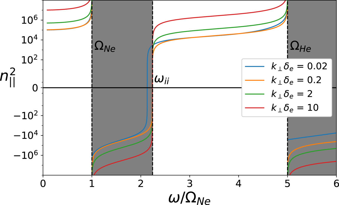
Figure 1. Dispersion relation of the shear Alfvén wave, for an evenly mixed He/Ne plasma. Dashed lines mark the locations of the ion cyclotron resonance frequencies and ion–ion hybrid cutoff frequency. At sufficiently large  $k_\perp$, the cutoff frequency converges to the ion–ion hybrid frequency $\omega _{ii}$. Greyed out regions indicate regions of evanescence in the large- $k_\perp$ limit.
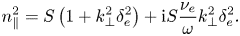
The cutoff frequency of the shear wave was numerically found from (2.3) for a wide range of  $k_\perp$, for several different mixes of He/Ne, and the results are shown in figure 2. It can be seen that at sufficiently large $k_\perp \delta _e$, the cutoff frequency converges to a fixed value, denoted by a dashed line. An analytic expression for the asymptotic limit of the cutoff frequency can be found by considering the limit where $n_\perp ^2 \gg |S|, |D|$, a condition that is easily satisfied in typical LAPD antenna experiments (aside from a narrow band of frequencies around either ion cyclotron resonance). In this limit, the shear wave branch of the dispersion relation given by (2.3) can be approximated by the following:
 \begin{equation} n_\parallel^2 = S \left( 1+ k_\perp^2 \delta_e^2 \right) + \textrm{i} S \frac{\nu_e}{\omega} k_\perp^2 \delta_e^2 . \end{equation}
An interesting observation of (2.4) is that, for the relatively large values of  $k_\perp$ assumed, the $E \times B$ slippage current plays a negligible role in the cross-field dynamics compared with the ion polarization current. Thus, in the limit of large $k_\perp$, the shear wave is mediated entirely by the ion polarization and parallel electron currents. Previous studies of shear waves (Morales, Loritsch & Maggs Reference Morales, Loritsch and Maggs1994) have shown that the $E \times B$ slippage current vanishes at low frequency (which can be seen by inspection of (2.2)), which physically corresponds to all particle species having the same $E \times B$ drift, resulting in no net current. Although this assumption is not true for the frequencies considered here (namely, in the upper band), the relatively large values of $k_\perp$ being imposed by our antenna results in the $E \times B$ current ultimately playing a similarly negligible role in the dispersion of the wave. Equation (2.4) is commonly known as the dispersion relation of the inertial Alfvén wave.
Figure 2. Cutoff frequency of the shear wave as a function of  $k_\perp$ in a two-ion species plasma, for several mixes of helium/neon. When $k_\perp \delta _e$ is sufficiently large, the cutoff frequency converges to an asymptotic value that is equal to the ion–ion hybrid frequency for that mix ratio (denoted by a dashed line).
For plasmas with weak collisionality ( $\nu _e \ll \omega$), the real parallel wavenumber $k_\parallel$ for a two-ion species inertial Alfvén wave can be written as follows:
 \begin{equation} k_\parallel^2 = \frac{\omega^2}{c^2} \frac{(\omega_{p1}^2+\omega_{p1}^2)(\omega^2 - \omega_{ii}^2)}{(\varOmega_{c1}^2-\omega^2)(\omega^2 - \varOmega_{c2}^2)} \left( 1+ \delta_e^2 k_\perp^2 \right),\quad \text{where} \ \omega_{ii}^2 = \frac{\varOmega_{c1}^2 \omega_{p2}^2 + \varOmega_{c2}^2 \omega_{p1}^2 }{\omega_{p1}^2 + \omega_{p2}^2} . \end{equation}
In (2.5),  $\omega _{ii}$ is the ion–ion hybrid frequency, and corresponds to the asymptotic limit of the cutoff frequency seen in figure 1. It was first discovered as a resonance for cross-field propagation (Buchsbaum Reference Buchsbaum1960), although in the context of parallel propagation we see that it acts as a cutoff. As $\omega _{ii}$ is found from the root of $S$, physically this corresponds to the frequency where the ion polarization currents of the two ion species are equal in magnitude and oscillate ${\rm \pi}$ out of phase, resulting in no net cross-field current. The ion–ion hybrid cutoff frequency is of interest to us as a potential diagnostic, and for singly charged ions it can be rewritten to be a function of the ion density ratio:
 \begin{equation} \frac{\omega_{ii}}{\varOmega_2} = \sqrt{ \displaystyle\frac{1+\displaystyle\frac{m_2}{m_1} \displaystyle\frac{n_2}{n_1}} {1+ \displaystyle\frac{m_1}{m_2} \displaystyle\frac{n_2}{n_1} } } . \end{equation}
As doubly charged ions have a different charge-to-mass ratio, they effectively contribute additional ion species to the plasma, although for the experimental conditions considered in this paper it is sufficient to assume only singly ionized particles are present in the plasma. Equation (2.6) suggests that measurement of the ion–ion hybrid cutoff frequency could, in principle, be used to resolve the ratio of ion densities. The ability to locally measure  $\omega _{ii}$ would provide a valuable diagnostic and is the primary motivation for the present study. This has been investigated previously by Vincena et al. (Reference Vincena, Farmer, Maggs and Morales2013) in a hydrogen–helium plasma, where the power spectrum was measured in order to infer the value of the cutoff frequency. In addition, previous investigations have attempted to measure $\omega _{ii}$ in the context of cross-field resonance, both as an impurity diagnostic (Chen et al. Reference Chen, Dimonte, Christensen, Neil and Romesser1986) as well as for evenly mixed plasmas (Watson et al. Reference Watson, Heidbrink, Burrell and Kramer2004).
Generally speaking, an antenna's power will be distributed across a continuous spectrum of  $k_\perp$ waves, each with their own respective cutoff frequency, as seen previously in figure 2. The full waveform is then found from the aggregate sum of these different $k_\perp$ waves. For an azimuthally symmetric wave, this can be expressed mathematically as follows:
 \begin{equation} E_j(r,z,t) = \exp({-\textrm{i}\omega t}) \int_0^\infty C(k_\perp) J_1(k_\perp r) \exp({\textrm{i} k_\parallel(k_\perp) z}) k_\perp \,\textrm{d} k_\perp + \textrm{c.c.}, \end{equation}
where  $C(k_\perp )$ is, in general, set by the boundary conditions of the antenna used to excite the wave (Morales et al. Reference Morales, Loritsch and Maggs1994; Morales & Maggs Reference Morales and Maggs1997). This would normally be problematic for an experimenter that wishes to measure the cutoff frequency, as each value of $k_\perp$ will contribute its own unique cutoff. If the majority of wave power imposed by an antenna, however, is contained at large values of $k_\perp$, where $\omega _{\textrm {cut}} \sim \omega _{ii}$, the cutoff frequency should be fairly robust as a measurable quantity. Deviations from the large $k_\perp$ limit, even in a small part of the antenna's $k_\perp$ spectrum, will result in some ‘filling in’ of the propagation gap seen in figure 1. Therefore, an idealized diagnostic for measuring the ion–ion hybrid cutoff frequency should be constructed such that it imparts nearly all of its power at values of $k_\perp$ which satisfy $n_\perp ^2 \gg |S|, |D|$, where the inertial Alfvén dispersion limit of (2.5) holds.
In the limit  $k_\perp \delta _e \rightarrow 0$, where our previous assertion $n_\perp ^2 \gg |S|,|D|$ breaks down, we see from figure 2 that the cutoff diverges from $\omega _{ii}$. In this limit, the inertial branch turns into the right-handed wave $n_\parallel ^2 = S+D$, which has no cutoff frequency in the ion cyclotron regime. The fast wave branch turns into the left-handed wave $n_\parallel ^2 = S - D$, which has the following cutoff frequency for a two-ion species plasma:
 \begin{equation} \omega_{\textrm{cut}} = \frac{\varOmega_{c1}^2 \omega_{p2}^2 + \varOmega_{c2}^2 \omega_{p1}^2 }{\varOmega_{c1}\omega_{p2}^2 + \varOmega_{c2} \omega_{p1}^2} . \end{equation}
Although the present study only considers waves whose energy is almost entirely contained in values of  $k_\perp$ where the inertial Alfvén wave dispersion holds, it is worth mentioning that (2.8) can similarly be written in terms of $n_2/n_1$ and therefore be used as a diagnostic as well. Watson et al. (Reference Watson, Heidbrink, Burrell and Kramer2004) explored this cutoff frequency as a diagnostic tool, although it was again in the context of cross-field propagation.
2.1 Kinetic considerations: thermal effects
The derivation of  $\omega _{ii}$ as a parallel cutoff frequency in the preceding section is predicated on the assumption that the plasma can be treated as a perfectly cold fluid. If we are to develop a diagnostic around measuring the ion–ion hybrid cutoff frequency, it is in our interest to determine under which plasma conditions $\omega _{ii}$ fails to accurately approximate the two-ion cutoff frequency. The purpose of this section is to determine the behaviour of the two-ion cutoff frequency when plasma effects outside the scope of the cold plasma model are considered.
In the context of kinetic theory, deviations from cold fluid theory fall under two major categories: ion FLR and thermal effects. We first consider a plasma with negligible FLR effects but arbitrary temperature, whose dielectric components can be written as follows:
 \begin{equation} \left.\begin{gathered} \varepsilon_\perp = \frac{1}{2}\sum_{s} \frac{\omega_{ps}^2}{\omega^2} \zeta_{0,s} \left[ Z(\zeta_{1,s}) + Z(\zeta_{-1,s}) \right], \\ \varepsilon_{xy} = \frac{i}{2}\sum_{s} \frac{\omega_{ps}^2}{\omega^2} \zeta_{0,s} \left[ Z(\zeta_{1,s}) - Z(\zeta_{-1,s}) \right], \\ \varepsilon_\parallel = - \sum_{s} \frac{\omega_{ps}^2}{\omega^2} \zeta_{0,s}^2 Z^{\prime}(\zeta_{0,s}), \end{gathered}\right\} \end{equation}
where  $\zeta _{n,s} \equiv (\omega - n \varOmega _{{cs}})/\sqrt {2} k_\parallel v_{{Th},s}$, $Z(\zeta )$ is the plasma dispersion function, and the summations are over all particle species $s$. We retrieve the cold plasma dielectric of (2.2) in the limit $|\zeta _{n,s}| \gg 1$. In many laboratory plasmas, such as those found in the LAPD, this is generally satisfied for the ions but not the electrons. In the cross-field direction, it can be shown that the electron contribution to $\varepsilon _\perp$ can be ignored so long as $|\varOmega _{{ce}}| \gg \sqrt {2} k_\parallel v_{{Th},e}$ is satisfied. In the parallel direction, the ion contribution can be ignored as well. Therefore, the only manifestation of kinetic electrons in the dielectric tensor is in modifying the parallel electron current, and the previously derived dispersion relation (2.4) can be generalized accordingly to give the following:
 \begin{equation} n_\parallel^2 = \varepsilon_\perp \left( 1 - \frac{n_\perp^2}{\varepsilon_\parallel} \right) = S \left( 1 + \frac{\delta_e^2 k_\perp^2}{\zeta_{0,e}^2 Z^\prime \left( \zeta_{0,e} \right) } \right) . \end{equation}
In the limit of hot, or adiabatic, electrons,  $|\zeta _{0,e}| \ll 1$ and $Z^\prime (\zeta ) \approx -2$. Substituting this expression into (2.10) and solving for $n_\parallel ^2$, we obtain the following dispersion for shear Alfvén waves in the limit of adiabatic electrons:
 \begin{equation} n_\parallel^2 = \frac{S}{1 + Sk_\perp^2 \lambda_{\textrm{De}}^2} , \end{equation}
where  $\lambda _{\textrm {De}}$ is the electron Debye length of the plasma. Equation (2.11) is known as the kinetic Alfvén wave. We see that the root of the kinetic Alfvén wave still corresponds to $S=0$, meaning $\omega _{ii}$ is still a valid approximation for the cutoff even in the limit of hot electrons. Next, we wish to determine the cutoff behaviour for intermediate values of $\zeta _{n,s}$, where kinetic effects such as Landau resonance are expected to play a larger role. Previous attempts to measure the parallel dispersion for shear waves with finite $k_\perp$ (Kletzing et al. Reference Kletzing, Thuecks, Skiff, Bounds and Vincena2010) found that a fully generalized complex kinetic solution had the best agreement with experimental data in the LAPD. For simplicity, we continue to assume our dispersion is mediated by cold ions across the field and kinetic electrons along the field, and focus on solving (2.10) numerically for $k_\parallel (\omega )$. The Newton–Raphson root-finding method was employed in order to solve (2.10) numerically (Ypma Reference Ypma1995). For most frequencies, the cold plasma dispersion (2.4) was found to be a satisfactory initial estimate of the root in order to allow the algorithm to converge. For frequency bands where $|\zeta | \ll 1$, however, the kinetic dispersion (2.11) was used as an initial estimate of the root instead.
Figure 3(a) shows  $k_\parallel (\omega )$, as found numerically from (2.10), alongside its inertial (2.4) and kinetic (2.11) limits. A 50 % He/50 % Ne plasma was considered, with $B_0 = 1500$ G, $T_e = 5$ eV, $n_e = 10^{12}\ \textrm {cm}^{-3}$ and $\lambda _\perp = 4$ cm. In the lower band, the numerical solution most closely matches the kinetic Alfvén wave dispersion. We see that the cutoff frequency is identical for all three dispersion relations, and that the exact solution converges with the inertial Alfvén wave close to the cutoff. This is expected, as the $|\zeta | \gg 1$ cold plasma limit is by definition always satisfied near the cutoff, because $k_\parallel \rightarrow 0$. A spatial damping, given by the imaginary part of $k_\parallel (\omega )$, is present at all frequencies and is indicated by the dashed lines in figure 3. Although the damping is small for most frequencies, it becomes substantial close to either resonance frequency and should be accounted for in a laboratory setting. Note that as we have not included ion cyclotron damping in our model, this damping is due entirely to parallel electron particle–wave interactions in response to the wave's large $k_\parallel$.
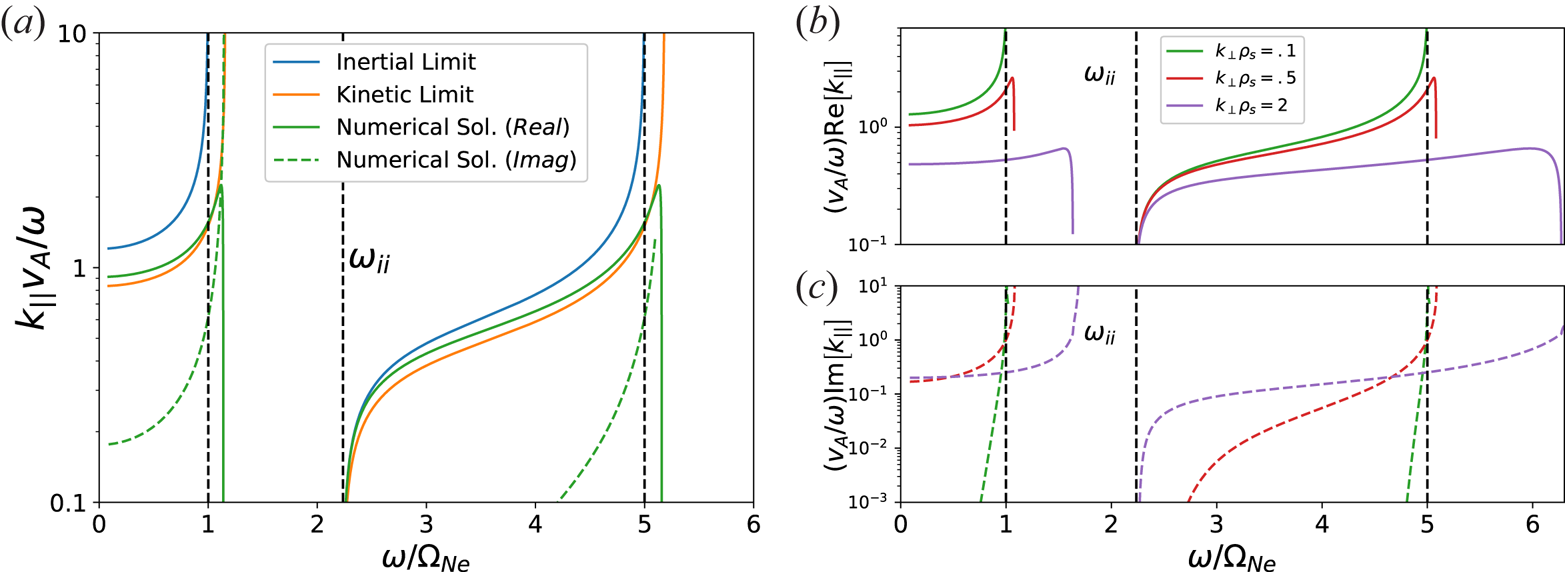
Figure 3. (a) Dispersion relation for a 50 % He/50 % Ne plasma with cold ions and warm electrons, compared with the cold and hot limits of the dispersion. Dashed lines mark the ion cyclotron resonance frequencies and ion–ion hybrid frequency. (b) Real parallel wavenumber and (c) spatial damping, for several different electron temperatures.
Figures 3(b) and 3(c) show the predicted wavenumber and spatial damping, respectively, for several different values of  $k_\perp \rho _s$, where $\rho _s$ is the root-mean-squared ion sound gyroradius of the system, defined by
 \begin{equation} \rho_s^2 \equiv \sum_{\textrm{ions}} f_i \rho_{s,i}^2 = \sum_{\textrm{ions}} \frac{n_i}{n_e} \frac{c_{s,i}^2}{\varOmega_{{ci}}^2} , \end{equation}
where  $f_i$ is the fractional ion concentration and $c_{s,i} = \sqrt {T_e/m_i}$ is the ion sound speed of species $i$. An interesting observation is that the existence of increasingly kinetic electrons pushes the boundary of both propagation bands past the ion cyclotron resonance frequencies. It can be seen in figure 3 that the upper bound of both propagation bands are identical for the kinetic Alfvén wave as well as the exact solution, although the inclusion of electron Landau damping smooths over the resonance and prevents it from diverging to infinity. Therefore, an analytic expression for the frequency shift of the resonance for either species can be found from the resonances of (2.11), and for small deviations from the ion cyclotron frequency are given by the following:
 \begin{equation} \omega_{\textrm{Res},i}^2 = \varOmega_{{ci}}^2 + k_\perp^2 f_i c_{s,i}^2 . \end{equation}
Although increased  $k_\perp \rho _s$ permits propagation at frequencies past the ion cyclotron frequencies, figure 3(c) suggests that waves in these regions will be heavily damped. But regardless of resonance behaviour, figure 3 shows that the cutoff frequency is unchanged in the presence of thermal electron effects, lending credence to its viability as a diagnostic for a wide range of electron temperatures.
2.2 Kinetic considerations: ion FLR effects
In this section we consider the behaviour of the two-ion cutoff frequency in a cold plasma, but with arbitrary ion FLR effects. FLR effects can be ignored when  $k_\perp \rho _i \ll 1$, where $\rho _i$ is the gyroradius of particle species $i$. This condition is usually satisfied in LAPD plasmas, but there are some plasma/antenna conditions where this inequality may not hold.
The inclusion of FLR effects means we must include the additional off-diagonal dielectric terms that were previously ignored in establishing (2.1a,b). As we showed in the previous section that the cutoff frequency is the same for all electron temperatures, we consider the ‘cold’ limit ( $Z(\zeta ) \rightarrow -1/\zeta$) for all particle species, while retaining ion FLR effects. The caveat to this assumption is that it is not valid for frequencies very close to the ion cyclotron resonance frequencies, although it is easily satisfied for frequencies in the vicinity of the cutoff. We continue to assume negligible electron FLR effects, as well as only considering frequencies $\omega \ll |\varOmega _{ce}|$. In addition, we rotate our coordinates such that $\boldsymbol {n} = n_\perp \hat {x} + n_\parallel \hat {z}$. The generalized version of (2.1a,b) can then be written as
 \begin{equation} \begin{bmatrix} \varepsilon_{xx} - n_\parallel^2 & \varepsilon_{xy} & \alpha n_\parallel + n_\perp n_\parallel \\ -\varepsilon_{xy} & \varepsilon_{yy} - n_\parallel^2 - n_\perp^2 & \beta n_\parallel \\ \alpha n_\parallel + n_\perp n_\parallel & -\beta n_\parallel & \varepsilon_{zz} - n_\perp^2 \end{bmatrix} \cdot \begin{pmatrix} E_x \\ E_y \\ E_z \end{pmatrix} = 0 , \end{equation}
where
 \begin{equation} \left.\begin{gathered} \varepsilon_{xx} = - 2 \sum_{\textrm{ions}} \omega_{{pi}}^2 \frac{\textrm{e}^{-\lambda_i}}{\lambda_i} \sum_{n=1}^{\infty} \frac{n^2 I_n}{\omega^2 - (n \varOmega_{{ci}})^2} ,\\ \varepsilon_{xy} = -\textrm{i}\frac{\omega_{{pe}}^2}{\omega \left| \varOmega_{{ce}} \right| } - 2 \textrm{i} \sum_{\textrm{ions}} \frac{\varOmega_{{ci}}}{\omega} \omega_{{pi}}^2 \, \textrm{e}^{-\lambda_i} \sum_{n=1}^{\infty} \frac{ n^2 (I_n^{\prime} - I_n)}{\omega^2 - (n \varOmega_{{ci}})^2} ,\\ \varepsilon_{yy} = \varepsilon_{xx} - 2 \frac{\omega_{{pe}}^2}{\omega^2} \frac{k_\perp^2 v_{{Th},e}^2}{\varOmega_{{ce}}^2} + 2 \sum_{\textrm{ions}} \frac{\omega_{{pi}}^2}{\omega} \lambda_i \,\textrm{e}^{-\lambda_i} \sum_{n=-\infty}^{\infty} \frac{I_n^{\prime} - I_n}{\omega - n\varOmega_{{ ci}}} ,\\ \varepsilon_{zz} = -\frac{\omega_{{ pe}}^2}{\omega^2} ,\\ \alpha = -\frac{4}{n_\perp} \sum_{\textrm{ions}} \omega_{{pi}}^2 \varOmega_{{ci}}^2 \,\textrm{e}^{-\lambda_i} \sum_{n=1}^{\infty} \frac{n^2 I_n}{\left[ \omega^2 - (n\varOmega_{{ci}})^2\right]^2} ,\\ \beta = -\textrm{i} n_\perp \frac{\omega_{{ pe}}^2 v_{{ Th},e}^2}{c^2 | \varOmega_{{ ce}}| \omega} + \textrm{i} k_\perp \sum_{\textrm{ions}} \frac{\omega_{{ pi}}^2 v_{{ Th},i}^2}{c \varOmega_{{ ci}}} \,\textrm{e}^{-\lambda_i} \sum_{n=-\infty}^{\infty} \frac{I_n^{\prime} - I_n}{(\omega - n\varOmega_{{ ci}})^2} , \end{gathered}\right\} \end{equation} $\lambda _i \equiv (k_\perp \rho _i / \varOmega _{{ ci}})^2$ and $I_n = I_n (\lambda _i)$ is the modified Bessel function of order $n$. Note that we redefined the dielectric terms $\varepsilon _{xz} \equiv \alpha n_\parallel$ and $\varepsilon _{yz} \equiv \beta n_\parallel$, where $\alpha$ and $\beta$ are independent of $k_\parallel$. In this way, all the terms defined in (2.15) are independent of $k_\parallel$ and the $n_\parallel$ dependence of (2.14) is shown explicitly. Although we chose to cast (2.14) in Cartesian coordinates, the system of equations is directly analogous to cylindrical coordinates via the variable substitutions $\hat {x} \rightarrow \hat {r}$ and $\hat {y} \rightarrow \hat {\theta }$, therefore any analysis performed in Cartesian coordinates is directly transferable to a cylindrical system with azimuthal symmetry.
The dispersion relation of the system is found by taking the determinant of (2.14), and the resulting characteristic equation is a quadratic in  $n_\parallel ^2$:
 \begin{equation} 0 = A n_\parallel^4 - B n_\parallel^2 + C , \end{equation}
where
 \begin{equation} \left.\begin{gathered} A = \varepsilon_{zz} + \alpha^2 - \beta^2 + 2 \alpha n_\perp ,\\ B = (\varepsilon_{yy} - n_\perp^2)(\varepsilon_{zz} + \alpha^2 + 2\alpha n_\perp) + \varepsilon_{xx}(\varepsilon_{zz} - n_\perp^2 - \beta^2) - 2\beta \varepsilon_{xy} (\alpha + n_\perp) ,\\ C = (\varepsilon_{zz} - n_\perp^2)\left[\varepsilon_{xx}(\varepsilon_{yy} - n_\perp^2) + \varepsilon_{xy}^2\right]. \end{gathered}\right\} \end{equation}
Equation (2.16) can then be readily solved for  $k_\parallel (\omega , k_\perp )$, using the definitions provided by (2.17) and (2.15), without having to resort to numerical root-finding methods.
Figure 4 shows the resulting dispersion relation for a 50 % He/50 % Ne plasma, where we have assumed the same plasma conditions as in figure 3 (in addition to  $T_i = 1$ eV for both ion species). This corresponds to $k_\perp \rho _i \sim 0.5$ for the heavier of the two ion species, and so FLR effects are expected to be present but not dominating. The first major change we see is the emergence of an additional propagating band, bounded by $1.73 \varOmega _\textrm {Ne} < \omega < 2\varOmega _\textrm {Ne}$, in a frequency regime that was evanescent previously. Hints of this propagation band have been observed in previous experiments (Vincena et al. Reference Vincena, Morales and Maggs2010, Reference Vincena, Farmer, Maggs and Morales2013), and was speculated to be due to an ion Bernstein mode-like feature. This feature effectively ‘fills in’ part of the previously evanescent region, defined by $\varOmega _\textrm {Ne} < \omega < \omega _{ii}$, which may make it difficult to experimentally identify the cutoff frequency. Additional frequency bands can be seen at higher harmonics of the neon cyclotron frequency.
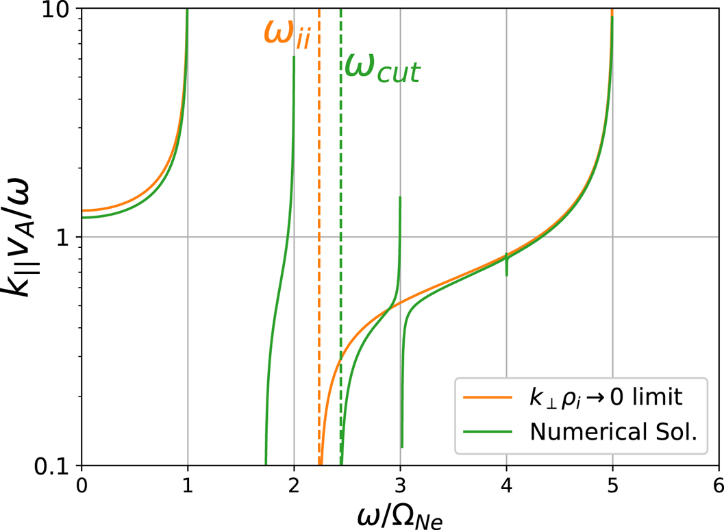
Figure 4. Real parallel wavenumber for the inertial Alfvén wave in a 50 % He/50 % Ne plasma, with and without ion FLR effects included in the dielectric tensor. Vertical dashed lines from, left to right, denote the ion–ion hybrid frequency and the shifted cutoff frequency in the presence of FLR effects.
An additional change to the dispersion relation in figure 4 is that the cutoff frequency is shifted, from  $\omega _{ii}$ ( ${\sim } 2.24 \varOmega _\textrm {Ne}$) to about $2.43 \varOmega _\textrm {Ne}$. If the mix ratio were calculated from this measured cutoff frequency without accounting for FLR effects (via (2.6)), the resulting estimate of the ion mix would be closer to $56\,\%$ neon, differing substantially from the actual mix ratio. Therefore FLR effects clearly have a severe impact on the accuracy of such a diagnostic. In the limit $k_\perp \rho _i \rightarrow \infty$ (which can be computed using the asymptotic form of $I_n \sim \textrm {e}^{\lambda _i}/\sqrt {2 {\rm \pi} \lambda _i}$), there is no cutoff frequency as all previously evanescent frequency bands can now facilitate propagation.
It is clear that FLR effects have a noticeable effect on the ion–ion cutoff frequency, and so our next goal is to explicitly determine the dependence of the cutoff frequency on  $k_\perp$. Assuming a parameter regime where $n_\perp ^2$ is much greater than the individual terms of the dielectric tensor (with the exception of the parallel dielectric $\varepsilon _{zz}$, which can be comparable with or greater than $n_\perp ^2$), we can expand (2.16) accordingly and derive an analytic expression for the dispersion relation to lowest order. The result is the following:
 \begin{equation} n_\parallel^2 = \varepsilon_{xx}\left( 1 + k_\perp^2 \delta_e^2\right) , \end{equation}
where  $\varepsilon _{xx}$ is defined in (2.15). Equation (2.18) is analogous to the inertial Alfvén dispersion, given by (2.4), and so can be thought of as the dispersion relation for inertial Alfvén waves with finite FLR effects.Footnote 1 The cutoff frequency corresponds to the root(s) of $\varepsilon _{xx}$, or
 \begin{equation} \sum_{\textrm{ions}} \omega_{{ pi}}^2 \frac{\textrm{e}^{-\lambda_i}}{\lambda_i} \sum_{n=1}^{\infty} \frac{n^2 I_n (\lambda_i)}{\omega^2 - (n\varOmega_{{ ci}})^2} = 0 . \end{equation}
Equation (2.19) will presumably contain multiple roots, owing to the higher harmonic resonances. As we are specifically interested in perturbations to the ion–ion cutoff frequency, we limit ourselves to finding the root within the frequency band bounded by the nearest harmonics above and below  $\omega _{ii}$ (i.e. for a 50 % He/50 % Ne plasma, where $\omega _{ii} \approx 2.24 \varOmega _\textrm {Ne}$, we would look for the cutoff in the frequency band $2 \varOmega _\textrm {Ne} < \omega < 3 \varOmega _\textrm {Ne}$).
Figure 5 shows the two-ion cutoff frequency ( $\omega _{\textrm {cut}}$) as a function of $k_\perp \rho _\textrm {Ne}$ in a helium–neon plasma, where $\rho _\textrm {Ne}$ is the neon gyroradius. Note that the values of $k_\perp \rho _\textrm {Ne}$ shown in figure 5 reside within the asymptotic region of figure 2, meaning any deviation of the cutoff from $\omega _{ii}$ (denoted by a horizontal dashed line) is entirely due to FLR effects, and is a separate phenomena from the $k_\perp \delta _e$ scaling that was discussed previously. For all three mixes shown in figure 5, the cutoff frequency approaches its respective ion–ion hybrid frequency in the $k_\perp \rho _\textrm {Ne} \rightarrow 0$ limit, as expected. In the intermediate region, where $k_\perp \rho _\textrm {Ne} \sim 1$, the cutoff frequency deviates significantly from the ion–ion hybrid frequency. In the limit where $k_\perp \rho _\textrm {Ne} \rightarrow \infty$, the cutoff frequency approaches the nearest ion cyclotron harmonic. In this limit, FLR effects completely fill in the evanescent gaps in the dispersion, allowing propagation at virtually all frequencies. Therefore, accurate measurement of the ion–ion hybrid frequency becomes significantly more challenging with increasing $k_\perp \rho _i$.
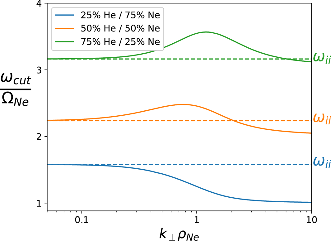
Figure 5. Two-ion cutoff frequency of the inertial Alfvén wave as a function of increasing FLR effects, for several mixes. The horizontal dashed line denotes the ion–ion hybrid frequency for its respective mix, which the cutoff frequency converges to in the limit  $k_\perp \rho _i \rightarrow 0$.
An interesting consequence of this analysis is that although  $\varepsilon _{xx} = 0$ gives the cutoff frequency as a function of $k_\perp$, it is also the dispersion relation for ion Bernstein waves (Schmitt Reference Schmitt1973). This suggests that an inertial Alfvén wave that is incident on an ion–ion hybrid cutoff layer in the plasma may spontaneously mode convert into an ion Bernstein wave (Swanson Reference Swanson1998). Ion Bernstein waves have been explored previously as a potential diagnostic for both ion temperature and ion minority concentration (Riccardi et al. Reference Riccardi, Fontanesi, Galassi and Sindoni1994).
2.3 Collisionality
Next we pose the question of how collisionality affects the ion–ion hybrid cutoff frequency. For simplicity, we again assume a cold, fluid-like plasma, in the regime where  $\omega _{ii}$ matches the cutoff frequency to good agreement. There are several types of ‘collisionality’, depending on the context: the kind we consider here is that responsible for bulk momentum transfer between particle species. To lowest order, the biggest change to the dielectric tensor is in adding an imaginary term to the parallel electron motion. This can be captured by modifying the parallel dielectric component to be $P = -\omega _{{ pe}}^2/\omega (\omega + \textrm {i} \nu _e)$, where $\nu _e$ is the total collision frequency for electrons with all other particle species, such as ions and neutrals.
As the cutoff frequency is found from either  $\varepsilon _{xx} = 0$ or $S = 0$, depending on whether FLR effects are taken into account or not, this suggests that, to lowest order, electron collisions have no effect on the two-ion cutoff frequency. Although collisions between ion species will modify the polarization current, and consequently the cutoff frequency, the ion–ion collision frequency in typical LAPD plasmas is well below the ion cyclotron frequencies and will thus have a negligible effect on wave damping.
2.4 Summary of theoretical results
To summarize the results of this section, we have demonstrated the existence of a cutoff frequency for parallel propagating waves in a two-ion species plasma, which exists between the two ion cyclotron resonance frequencies. For antennae of size of the order of the electron skin depth (i.e.  $k_\perp \delta _e \sim 1$) or smaller, this cutoff frequency can be approximated by the ion–ion hybrid frequency $\omega _{ii}$, which in turn can be expressed as a function of the ratio of ion densities. Therefore, the ion–ion hybrid frequency is of interest to us as a potential diagnostic tool in two-ion species plasmas.
The cutoff frequency was shown to be unchanged by electron thermal effects, suggesting that a diagnostic based on measuring  $\omega _{ii}$ would be valid for all (reasonable) electron temperatures. It was shown, however, that the cutoff frequency deviates from $\omega _{ii}$ when $k_\perp \rho _i \ll 1$ is not satisfied, where $\rho _i$ is the ion gyroradius. In the presence of large ion FLR effects, it was shown that the cutoff frequency deviates from $\omega _{ii}$ and becomes a function of $k_\perp$, making it more difficult to apply such a diagnostic. An additional caveat of large ion FLR effects is that they tend to excite additional propagation bands near the cutoff, which may mask the exact value of the cutoff frequency and further limit this diagnostic's accuracy. Finally, the cutoff frequency was shown to be largely unaffected by electron collisionality. These results suggest that a diagnostic based on measuring $\omega _{ii}$ would be fairly robust under a wide range of plasma conditions, and could serve as a valuable tool in two-ion species plasmas.
3 Experimental set-up
3.1 General overview of LAPD
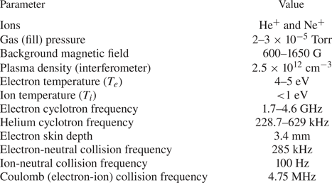
A series of experiments were conducted in the LAPD at UCLA. The LAPD is a cylindrical stainless steel chamber that is 18 m in length and 1 m in diameter. The chamber is surrounded by 56 electromagnets, capable of producing a highly uniform axial magnetic field  $(\delta B / B_0 < 0.5\,\%)$ up to 3000 G (Gekelman et al. Reference Gekelman, Pribyl, Lucky, Drandell, Leneman, Maggs, Vincena, Van Compernolle, Tripathi and Morales2016). A DC discharge is applied to a barium oxide (BaO)-coated cathode, located on one end of the machine. This produces a stream of primary electrons that pass through a 50 % transparent mesh anode, located 52 cm away, ionizing the gas throughout the rest of the chamber. The discharge lasts 12 ms, and is fired at a rate of 1 Hz to create a highly reproducible plasma. An overview of general plasma parameters for this experiment is listed in table 1.
Table 1. Range of plasma parameters considered in this experiment.
A gas feed system is installed in the centre of the machine, capable of supplying the chamber with steady rates of hydrogen, helium, neon and argon. Each gas is connected to its own mass flow controller (MFC), allowing precise control over the gas mix, and the partial pressures of each gas is measured using a residual gas analyser (RGA). This experiment explores the behaviour of shear Alfvén waves for various mix ratios of helium and neon. Throughout this paper, the neutral pressure ratio is used as a proxy for estimating the ion density ratio of the plasma. Although it is not assumed (or even expected) that these two quantities be equal, it serves as a satisfactory reference point as we investigate different mixes.
3.2 Antenna and probes
Shear Alfvén waves were excited using the rotating magnetic field (RMF) antenna (figure 6), originally designed to study circularly polarized waves (Gigliotti et al. Reference Gigliotti, Gekelman, Pribyl, Vincena, Karavaev, Shao, Sharma and Papadopoulos2009). The experiments described in this paper utilized only the horizontal loop of the antenna, which has a diameter of roughly 9 cm. The antenna was aligned such that the plane of the loop laid in the  $XZ$ plane. Previous experiments have shown that similar antenna configurations excite two antiparallel electron current channels, centred on either end of the loop. At frequencies well below the ion cyclotron resonance frequency, the induced magnetic field of this current configuration creates a plasma wave with a strong linearly polarized magnetic field $B_y$ along the background field line passing through the midpoint of the loop. A second dipole loop antenna was constructed with similar geometry, consisting of a 2.5 cm diameter insulated loop of wire mounted on a movable probe drive, and was used to launch shear Alfvén waves at varying radial positions in the plasma.

Figure 6. RMF antenna used to launch shear Alfvén waves, with cathode visible at the far end. Inset: Schematic of the antenna.
The antenna was driven by a sinusoidal waveform generator which was then fed through an RF amplifier to deliver several amps of current to the antenna. The amplitudes of the resulting Alfvén waves (measured several metres away) are of the order of tens of milligauss. Background fluctuations in the field due to plasma turbulence are typically of the order of tens of microgauss, resulting in a strong signal-to-noise ratio for the excited waves. Previous studies (Drozdenko & Morales Reference Drozdenko and Morales2001) on the LAPD have shown that large enough amplitude shear Alfvén waves can lead to wave current filamentation as well as modifications to the plasma density due to ponderomotive forces, but these nonlinear effects are only significant for wave magnitudes exceeding 10 % of the background field. Therefore, we are justified in using the linearized theory outlined in § 2.
Magnetic field fluctuations were measured with four three-axis magnetic induction (B-dot) probes, located at various axial positions in the plasma. Each component of the probes contains two, oppositely wound 25-turn coils, which were fed through a differential amplifier to subtract out any electrostatic pickup in the coil (Everson et al. Reference Everson, Pribyl, Constantin, Zylstra, Schaeffer, Kugland and Niemann2009). The locations of the probes, as well as the antenna, are shown in figure 7.
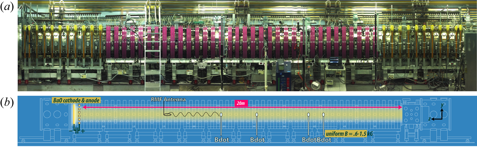
Figure 7. (a) Photograph and (b) schematic of LAPD, showing the location of the RMF antenna and probes.
4 Experimental results
4.1 General results
A series of frequency scans were performed under a wide range of plasma conditions, using the horizontal loop of the RMF antenna to excite a shear wave along the radial centre of the machine. The following measurements were taken with a series of B-dot probes, placed at various axial positions in the plasma along the radial centre of the machine (which we refer to as  $r=0$). In order to isolate the antenna-driven signal from the naturally occurring background turbulence of the plasma, the following formula is used throughout this paper to calculate the filtered power spectrum:
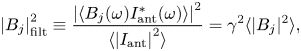 \begin{equation} \left| B_j \right|_{\textrm{filt}}^2 \equiv \frac{\left| \langle B_j(\omega) I_{\textrm{ant}}^* (\omega) \rangle \right|^2 }{\langle \left| I_{\textrm{ant}} \right|^2 \rangle} = \gamma^2 \langle | B_j |^2 \rangle , \end{equation}
where  $B_j$ is the measured (Fourier-transformed) B-dot signal in direction $j$,
$j$,  $I_{\textrm {ant}}$ is the antenna current and $\gamma (\omega )$ is the coherence between the B-dot signal and antenna current. An asterisk superscript denotes a complex conjugate, whereas the brackets denote an ensemble average. When background fluctuations are small relative to the antenna-driven signal, $\gamma \sim 1$ and the filtered power spectrum is identical to the regular power spectrum. Equation (4.1) is used in all power spectrum calculations that follow in this paper, and so the filt subscript is dropped in our notation. In addition, the spectra throughout this paper are normalized to the antenna current $I_{\textrm {Ant}}$, as the current provided by the RF power supply was not constant for all frequencies.
Figure 8 shows the power spectrum of the wave as a function of frequency, for varying background field strengths, at two axial positions. All cases are for a plasma with equal fill pressures of helium and neon. Assuming the ion density ratio is equal to the fill pressure ratio, (2.6) predicts the ion–ion hybrid cutoff frequency to be  $\omega _{ii} = 2.24 \varOmega _\textrm {Ne}$, which is labelled in the plots by a vertical dashed line. Two distinct frequency bands are observed, which is in agreement with the predicted dispersion of figure 1. The measured normalized cutoff frequency is largely unvarying with changing background field, which is consistent with the predicted scaling given by (2.6). The low-frequency side of the propagation gap begins to fill in at 900 G, and even more so for the 600 G case. This is consistent with our theoretical prediction from figure 3(b), which says that as electrons become increasingly kinetic, the upper bounds of the propagation bands can push past their respective ion cyclotron resonance frequencies. Meanwhile, the high-frequency side of the propagation gap also experiences some ‘filling in’ around the expected cutoff. This is speculated to be attributed to the contribution from smaller- $k_\perp$ waves which have cutoff frequencies below $\omega _{ii}$ (which can be seen in figure 2), resulting in a leakage of some power below the ion–ion hybrid cutoff.
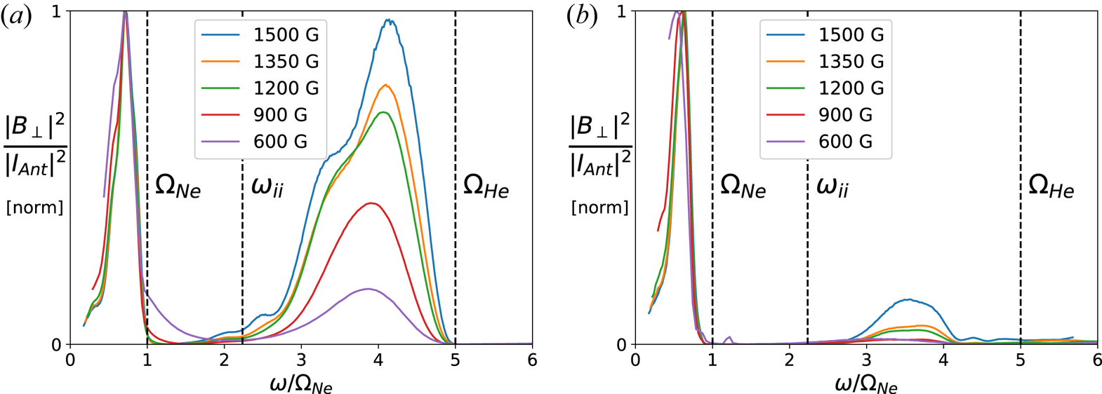
Figure 8. Normalized power spectrum of the perturbed magnetic field at (a) 3 m and (b) 9 m from the antenna, for various background fields, in a plasma with equal neutral pressures of helium and neon. Dashed lines, from left to right, mark the locations of the neon cyclotron resonance, ion–ion hybrid cutoff frequency (predicted value for a 50/50 mix), and helium cyclotron resonance.
Both the upper and lower frequency bands begin to lose power as they approach their respective resonance. This is consistent with our theoretical prediction in figure 3, which suggested that significant kinetic damping is expected just before either ion cyclotron resonance. In addition, previous studies (Morales et al. Reference Morales, Loritsch and Maggs1994) have shown that the ratio of perpendicular to parallel group velocities increases rapidly near the resonances, leading to a radial spreading of wave energy and consequently a smaller measured signal by the B-dot probe along  $r=0$. This behaviour has been observed in previous antenna experiments, both in the LAPD (Gekelman et al. Reference Gekelman, Leneman, Maggs and Vincena1994) as well as in a toroidal device (Borg et al. Reference Borg, Brennan, Cross, Giannone and Donnelly1985).
Having established the existence of a cutoff frequency which scales as expected with background field, our next objective is to vary the mix ratio of the plasma and see whether the cutoff frequency varies consistently with the scaling predicted by (2.6). Figures 9(a) and 9(b) show the power spectrum of the wave and parallel wavenumber, respectively, for various neutral fill pressure ratios in a background field of  $B_0 = 1500$ G. From (2.6), it is expected that $\omega _{ii}$ approaches $\varOmega _\textrm {He}$ with increasing neon concentration, and vice versa for increasing helium. This trend can be seen clearly in the power spectra of figure 9(a), where we have labelled the estimated cutoff frequencies with a coloured $X$. The measured spectra contain a small amount of power at all frequencies in the propagation gap, and so there is some ambiguity in identifying the location of the cutoff frequency. The cutoff frequency was identified either by a local minimum in the spectra, or the point where the slope is observed to rapidly increase. The upper band becomes weaker with decreasing helium (relative to the lower band), suggesting that the total power of the two propagating bands scale differently with ion mass. This is likely due to the fact that neon suffers higher collisional damping at these frequencies than helium. Several peaks can be seen in the spectra, especially for the majority-helium mixes. This has been observed before in the LAPD (Mitchell et al. Reference Mitchell, Vincena, Maggs and Gekelman2001), and it is suspected that this is due to backwards-propagating waves reflecting off the cathode and interfering with the forward propagating wave. Calculations using the phase velocity of the wave at these frequencies support this claim.
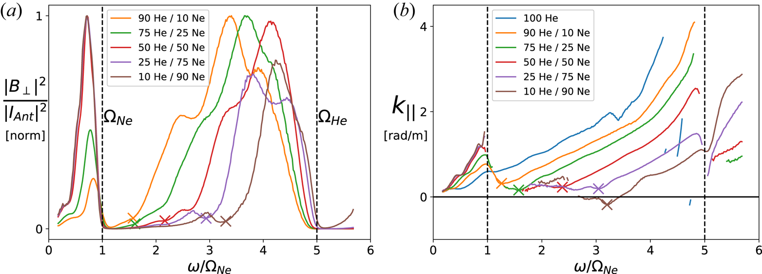
Figure 9. (a) Normalized power spectra and (b) parallel wavenumber, for various mix ratios of helium/neon for  $B_0 = 1500$ G. The crosses mark the estimated cutoff frequency, and were separately identified from both the measured spectra and dispersion. The different mix ratios shown are based on the neutral fill pressure of the gas, and not the ionized density ratio.
Figure 9(b) shows the parallel wavenumber, which was calculated from the cross-phase of two probes spaced 2.24 m apart axially (Smith & Powers Reference Smith and Powers1973), for various mix ratios.  $B_y$ was used to calculate the phase difference, as this component of the field had the strongest signal-to-noise ratio, but similar results are achieved using $B_x$. Data points which failed to meet a minimum coherence threshold of $\gamma ^2 > 0.9$ between the two probes were deemed too noisy and omitted from the plot. The results are in qualitative agreement with the predicted dispersion plotted in figure 1. Looking at the upper band in particular, we see $k_\parallel$ begin to increase past a certain frequency (presumably the cutoff frequency), rising rapidly and then eventually dropping as it approaches the ion cyclotron resonance. The cutoff frequency for each mixed case was estimated from the local minimum in the dispersion relation, and again labelled with an $X$. We observe that most of the measured wavenumbers do not actually cross the zero axis, but rather bottom out at a value above zero. This is speculated to be due to the finite length of the plasma column imposing a minimum fundamental eigenmode on the parallel wavelength, as discussed in Mitchell et al. (Reference Mitchell, Vincena, Maggs and Gekelman2001).
The two methods described previously, of inferring the cutoff from the local minima of either the power spectra or parallel dispersion, are successful in getting a rough estimate of the ion density ratio. Previous experiments on the LAPD have similarly determined the mix ratio of plasmas by looking at the measured power spectra (Vincena et al. Reference Vincena, Morales and Maggs2010). As we have shown in figures 8 and 9, however, there is a fair amount of subjectivity in these methods which severely limit the precision of the resulting measurements. In addition, data points in the vicinity of the cutoff are much more susceptible to noise, as the antenna-driven signal will, by definition, be close to zero. In § 4.3, we propose a much more rigorous method of determining the ion density ratio, which is done by numerically fitting the measured parallel wavenumber to the predicted dispersion curve.
4.2 Estimating the  $k_\perp$ spectrum from radial lines

A more rigorous method of determining  $\omega _{ii}$ would be to numerically fit the inertial Alfvén wave dispersion relation to the measured parallel wavenumber, as shown in figure 9. Before doing so, however, we would like some idea of the values of $k_\perp$ imposed by the antenna, which can be obtained from radial profiles of the wavefront.
Figure 10 shows the power spectrum of a wave launched in a 50 % He/50 % Ne plasma, measured at different radial offsets from the centre of the antenna. Owing to symmetry, the majority of wave power along this line is in  $B_y$, and so only the vertical component of the field is considered here. For the frequencies of interest, the peak power of the wavefront is located at the centre of the antenna. This is reassuring from a diagnostic point of view (and one of the reasons a magnetic loop antenna was chosen for this diagnostic), as there is no ambiguity in deciding where the B-dot probes should be placed relative to the antenna. The radial structure of the wavefronts seen in figure 10 is reminiscent of previous antenna experiments, in which two electrostatic disks were driven ${\rm \pi}$ out of phase with each other to drive two antiparallel electron current channels (Gekelman et al. Reference Gekelman, Leneman, Maggs and Vincena1994). Similarly, the RMF antenna induces two electron current channels running antiparallel to one another, located along the field lines passing through either side of the loop at $x = \pm 4.5$ cm. The resulting azimuthal field adds up constructively in between the two current channels, resulting in a strong vertically polarized wave at the midpoint of the antenna. This has been observed previously both in experiments (Gigliotti et al. Reference Gigliotti, Gekelman, Pribyl, Vincena, Karavaev, Shao, Sharma and Papadopoulos2009) with the same antenna as well as three-dimensional simulations (Karavaev et al. Reference Karavaev, Gumerov, Papadopoulos, Shao, Sharma, Gekelman, Wang, Van Compernolle, Pribyl and Vincena2011).
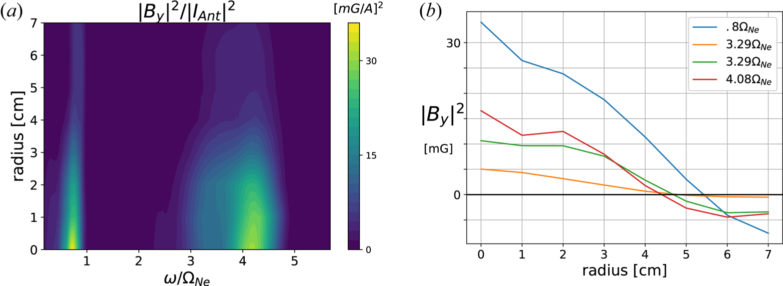
Figure 10. (a) Power spectrum of the wave 3 m from the antenna, for a 50 % He/50 % Ne plasma at 1500 G, measured at various radial distances from the centre of the plasma column. (b) Radial profiles of the vertical  $B$-field for several frequencies, taken at a time corresponding to the peak of the signal at $r = 0$.
Next, we wish to determine  $k_\perp$, as a function of $\omega$, from the radial profiles of figure 10. For simplicity, we assume the majority of the wave's power to be confined to a small range of $k_\perp$, such that the radial structure of the wavefront can be thought of as the superposition of two first-order Bessel functions centred on $R=\pm 4.5$ cm. Invoking the addition theorem of Bessel functions, we can express the net field of the two sources (along the horizontal plane) as being proportional to the following:
 \begin{equation} J_1\left(k_\perp\left(x+R\right)\right) - J_1\left(k_\perp\left(x-R\right)\right) = 4 \sum_{1,3,5\ldots} J_n\left(k_\perp R \right) J_n^\prime \left( k_\perp x \right) , \end{equation}
where  $x$ is the horizontal distance from the centre of the antenna and $R$ is the antenna's radius. To lowest order, the field is then given by $4J_1 (k_\perp R)J_1^\prime (k_\perp x)$, whose lowest root is approximately where $k_\perp x \approx 1.841$. From this, we are able to formulate a simple linear approximation for finding $\lambda _\perp$:
 \begin{equation} \lambda_\perp \approx 3.4126 x_0 , \end{equation}
where  $x_0$ is the horizontal position at which the vertical field of the wave crosses zero. Numerically, (4.3) was found to be accurate within 10 % for $k_\perp R <2.5$. Our method for estimating the value of $\lambda _\perp$, then, is as follows: find the time-instantaneous radial profile of the wave field (at a time corresponding to the peak of the wave), measure the position at which the field crosses zero and then use (4.3) to calculate $\lambda _\perp$. The results can be seen in figure 11(a), in which we have plotted the estimated $\lambda _\perp$ as a function of frequency. Figures 11(b) and 11(c) show a comparison of the measured radial profile to the profile predicted by (4.3), for two frequencies which are close to the peaks of the power spectra in the lower and upper band, respectively. It is straightforward to show that the condition $n_\perp ^2 \gg |S|, |D|$ is easily satisfied for nearly all measured values of $k_\perp$, and so the inertial Alfvén wave dispersion given by (2.4) holds.
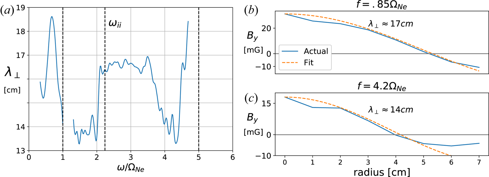
Figure 11. (a) Perpendicular wavelength versus frequency, estimated from the radial profiles of the field. Comparison of the measured radial profile to the predicted profile for (b)  $f = 0.85 \varOmega _\textrm {Ne}$ and (c) $f = 4.2 \varOmega _\textrm {Ne}$.
4.3 Determining the ion density ratio by fitting the measured parallel wavenumber
In this section we present a robust algorithm for efficiently fitting measured data of the parallel wavenumber to the theoretical prediction in order to determine the local ion density ratio. Consider an inertial Alfvén wave in a weakly collisional two-ion species plasma. The real parallel wavenumber, found from (2.5), can be written as follows:
 \begin{equation} k_\parallel \left( \bar{\omega} \right)^2 = - \frac{\omega_{p1}^2 + \omega_{p2}^2}{c^2} \frac{\bar{\omega}^2 \left(\bar{\omega}^2 - \bar{\omega}_{ii}^2\right)}{\left(\bar{\omega}^2 - 1\right)\left(\bar{\omega}^2 - m_{21}^2\right)} \left[1 + k_\perp^2 \delta_e^2\right], \end{equation}
where  $\bar {\omega } = \omega /\varOmega _{2}$ and $m_{21} = m_2/m_1$. We assume that $m_2$ refers to the mass of the heavier ion species, although the derivation that follows in this section works equally well if the opposite is assumed. Equation (4.4) can be rewritten in terms of the ion density ratio $\alpha = n_2/n_1$ as follows:
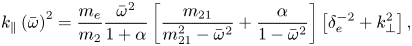 \begin{equation} k_\parallel \left(\bar{\omega}\right)^2 = \frac{m_e}{m_2} \frac{\bar{\omega}^2}{1+\alpha}\left[\frac{m_{21}}{m_{21}^2 - \bar{\omega}^2} + \frac{\alpha}{1-\bar{\omega}^2}\right]\left[\delta_e^{-2} + k_\perp^2\right], \end{equation}
where in deriving (4.5) we made use of the definition  $\bar {\omega }_{ii}^2 = m_{21}(1+m_{21}\alpha )/(m_{21}+\alpha )$, given by (2.6). Finally, we define the quantity $\beta ^2 = (m_e/m_2)(\delta _e^{-2} + k_\perp ^2)$ and rewrite our dispersion relation in the following form:
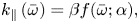 \begin{equation} k_\parallel \left(\bar{\omega}\right) = \beta f (\bar{\omega};\alpha), \end{equation}
where
 \begin{equation} f(\bar{\omega}; \alpha) = \frac{\bar{\omega}}{\sqrt{1+\alpha}}\left[\frac{m_{21}}{m_{21}^2 - \bar{\omega}^2} + \frac{\alpha}{1 - \bar{\omega}^2}\right]^{1/2} . \end{equation}
We have rewritten our dispersion relation in terms of two free parameters  $\alpha$ and $\beta$. We would like to find the values of $\alpha$ and $\beta$ which give us the best fit of (4.6) to the experimentally measured parallel wavenumber. We choose to quantify the fit using the least-squares error function, given by the following:
 \begin{equation} J = \frac{1}{N}\sum_{i} \left(y_i - k_\parallel\left(\bar{\omega}_{i}\right) \right)^2 , \end{equation}
where  $y_i$ is the measured parallel wavenumber, $k_\parallel (\bar {\omega }_i)$ is the predicted dispersion given by (4.6) and the sum is over all measured frequencies. At this point, the problem can be solved numerically in order to find the right combination of $\alpha$ and $\beta$ that minimizes the value of $J$ given previously. The problem can be simplified substantially, however, by solving for $\beta$ analytically. A common technique in regression problems is to take the partial derivative of the error function with respect to the free parameters and set it equal to zero in order to find the local minimum of the error function. Using (4.8), we can solve $\partial J/\partial \beta = 0$ to obtain the following expression for $\beta$:
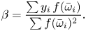 \begin{equation} \beta = \frac{\sum y_i\, f(\bar{\omega}_i)}{\sum f(\bar{\omega}_i)^2} . \end{equation}
By combining (4.9) with (4.6) and (4.7), we can express the predicted dispersion curve  $k_\parallel (\bar {\omega })$ in terms of a single free parameter $\alpha$. The final step, then, is to numerically find the value of $\alpha$ that minimizes the error function given by (4.8). A big advantage of this algorithm is that the dependence on the electron density and $k_\perp$ is contained entirely in the free parameter $\beta$, which we were able to solve for analytically. Therefore, we have developed an algorithm that is able to predict the ion density ratio without requiring any knowledge about the plasma density or $k_\perp$ spectrum. In addition, knowledge of the distance between the two probes is unnecessary as well, as this information can also be absorbed into our $\beta$ parameter.
Figure 12(a) shows the result of employing our best-fit algorithm to the measured dispersion for a 50 % He/50 % Ne plasma. Included in the plot is the numerical solution to the dispersion relation with kinetic effects included (found from (2.10)), to show that the inertial Alfvén wave dispersion is a more than acceptable approximation for the assumed plasma conditions. The best fit curve is obtained for a value of  $\alpha = 1.23$, or around 55.2 % neon. The best fit algorithm was applied only to the upper frequency band, that is, $\varOmega _{2} < \omega < \varOmega _{1}$). Two steps were taken in order to filter out noise before applying the best fit algorithm. The first step was to remove data points which had a low coherence with the antenna current (for this example, a threshold of $\gamma ^2 = 0.95$ was chosen). Second, frequencies where either one of the B-dot probe's power was less than 1 % of the maximum of the full-power spectrum (shown in figures 8a and 9a) were omitted from the fit as well. These two filtering steps ensure that only data points with a high signal-to-noise ratio are being used in order to fit the predicted dispersion. In addition, the parts of the spectrum below either ion cyclotron resonance where a drop in the measured wavenumber is observed were ignored, as these dips are not predicted by the cold plasma model and would otherwise add a large amount of unwanted error to the least-squares error function.
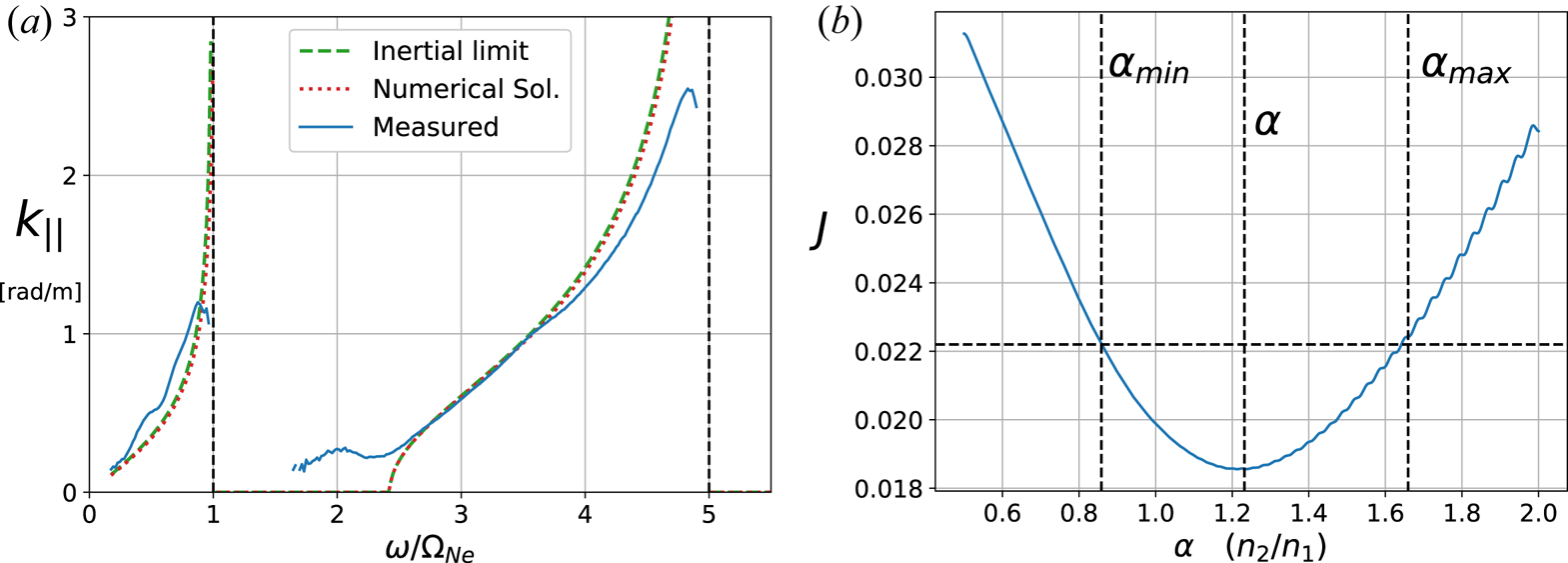
Figure 12. (a) Comparison of the measured dispersion, for a plasma with equal fill pressures of He/Ne, to the predicted dispersion relation of a shear Alfvén wave (both exact and in the cold limit). (b) Least-squares error function versus ion density ratio for the 50 % He/50 % Ne plasma. The error function is minimized for  $\alpha \approx 1.23$, corresponding to an ionized mix of 55.2 % neon. A 20 % increase from the minimum is used to estimate uncertainty, and gives error bars of 46–62 %.
In order to account for uncertainty in the measurements obtained by this algorithm, we propose the following technique. From the local minimum in the least-squares error function, find the values of  $\alpha$ on either side corresponding to a 20 % increase from the local minimum. These values determine the bounds of the error bars for the $\alpha$ measurement. Error functions with a sharp valley will have small error bars as a result, whereas error functions which are slow to find a minimum value will convey this information by having larger error bars. Figure 12(b) shows the error function versus $\alpha$ for the 50 % He/50 % Ne plasma. The predicted value of $\alpha$ as well as the minimum and maximum error bar values are denoted by dashed vertical lines. Note that the 20 % threshold that was used is arbitrary: although this value was found to give reasonable results for the dataset shown here, a different percentage threshold could be chosen if more or less error is desired.
Figure 13 shows how the method of least-squares fitting compares with the previously discussed methods of estimating the cutoff from the minimum of the power spectrum and dispersion. We see that the ion density ratios predicted from our best-fit algorithm scale consistently with what we would expect, validating the use of this method. The method was not able to find an adequate fit for the 90 % neon case, however, suggesting that this technique might struggle in situations where one of the ions is a minority species. However, for the other mix cases, this algorithm was successful in measuring an ion density ratio that is consistent with other methods and theoretical predictions.
Figure 13. Comparison of the three different methods discussed for finding the ion mix. The solid black line is the percentage of neon corresponding to if the ionized density ratio were to equal the neutral fill pressure.
4.4 Radial diagnostic for determining the ion density ratio
In this section we employ the algorithm derived in § 4.3 for determining the ion density ratio from the least-squares fit of the measured parallel wavenumber. A scaled down magnetic loop antenna was constructed, approximately 2.5 cm in diameter, and was used to launch shear waves at various radial positions in the plasma. At each radial position, the parallel wavenumber is measured and fit to the predicted dispersion curve to find the value of  $\alpha = n_2/n_1$ that yields the minimum least-squares error.
Figure 14 shows the result of applying our best-fit algorithm, outlined in the preceding section, to various radial positions in the plasma. The algorithm is performed by taking the predicted dispersion, given by (4.6), (4.7) and (4.9), and numerically finding the value of  $\alpha$ ( ${=}n_2/n_1$) that minimizes the least-squares error function given by (4.8). Only the frequencies in the upper band were considered for the fitting algorithm. We can see that the measured parallel wavenumbers for the first few positions in the plasma are in excellent agreement with the predicted dispersion curves. For positions near the edge of the plasma (around $r = 28$ cm), the fit is not as good although it is still able to estimate the ion density ratio in this region, although with greater uncertainty.
Figure 14. Measured parallel wavenumbers and the corresponding best-fit predicted dispersion, for various radial positions. Dashed vertical lines denote the corresponding location of the predicted ion–ion hybrid cutoff.
Figure 15 shows the estimated neon mix concentration versus radius in the plasma, for a plasma with equal fill pressures of helium and neon. Error bars were calculated from the values of  $\alpha$ corresponding to a 20 % increase from the local minimum in the least-squares error function. For positions $x \leqslant 20$ cm, the computed error bars are fairly small as the best fit plots are in excellent agreement with the measured parallel wavenumbers, as can be seen in figure 14. Figure 15 suggests that there is more ionized neon in the plasma (up to 65–70 % neon in the core) than the neutral pressure would suggest, which makes intuitive sense given that neon has a lower ionization potential than helium. The error bars are larger for positions $x > 24$ cm, which is understandable given the corresponding best-fit curves seen in figure 14. Overall, this diagnostic was successful in determining the ion density ratio as a function of position with relatively low error in the core of the plasma, while still giving reasonable estimates out in the edge.
Figure 15. Estimated percentage of ionized neon as a function of radius in the plasma, for a plasma with 50 % He/50 % Ne neutral pressure.
It should be noted that the reason the ionized density ratio in figure 15 differs so much from the 50 % He/50 % Ne case shown in figure 12 is that these measurements were taken in two different plasmas, several months apart, and although care was taken to reproduce similar plasma conditions, they are not expected to be identical.
5 Conclusion
The original purpose of this study was to investigate the ion–ion hybrid cutoff frequency of shear Alfvén waves in a two-ion species plasma, and evaluate its viability as a diagnostic for determining the ion density ratio. In § 2, theoretical work was done in order to expand the parameter regime in which such a diagnostic could be applied. We showed that for sufficiently large  $k_\perp \delta _e$, the cutoff frequency is identical to the ion–ion hybrid frequency $\omega _{ii}$, which can be expressed as a function of the ratio of ion densities. Numerical calculations demonstrated that this cutoff frequency was unchanged by kinetic thermal electron effects and very weakly varying with collisions, allowing this diagnostic to potentially be used in a wide range of plasmas. In plasmas with significant ion FLR effects (i.e.where $k_\perp \rho _i \ll 1$ is not satisfied), we showed that the cutoff frequency deviates from $\omega _{ii}$ and becomes a function of $k_\perp$, making it more difficult to apply such a diagnostic. An additional caveat of large ion FLR effects is that they tend to excite additional propagation bands near the cutoff, which may mask the exact value of the cutoff frequency and further limit this diagnostic's accuracy.
Shear Alfvén waves were systematically launched in a helium/neon plasma for a wide range of conditions in the LAPD. In § 4, we were able to demonstrate the existence of two distinct propagation bands bounded by  $\omega < \varOmega _\textrm {Ne}$ and $\omega _{ii}<\omega <\varOmega _\textrm {He}$. The cutoff frequency was measured from the local minima of both the power spectrum and parallel dispersion $k_\parallel ( \omega )$, and found to scale consistently with theory. Both methods of identifying the cutoff are limited in their precision, owing to the fact that the signal-to-noise ratio approaches zero near the cutoff frequency. In addition, non-ideal effects, such as filling in of the propagation gap due to low- $k_\perp$ waves, tend to obscure the precise value of the measured cutoff frequency. A robust algorithm was developed, which works by fitting the predicted dispersion relation to the measured $k_\parallel$ via minimization of the least-squares error, and finding the ion density ratio that yields the best fit. One of the advantages of this algorithm is that knowledge of the electron density, $k_\perp$ spectrum, or distance between probes is not required: a measurement of $k_\parallel$ as well as the background magnetic field is all that is required in order to determine the ion density ratio at a given position.
A diagnostic consisting of a magnetic loop antenna and two B-dot probes was applied in order to measure the parallel wavenumber as a function of radius in the plasma, and the least-squares fitting algorithm was applied in order to extract the radial profile of the ion species mix. These radially resolved measurements showed that for plasmas with equal helium and neon fill pressures, the ionized neon concentration was 65–70 % of the total ion density in the core, dropping to 50–60 % in the edge. Error bars were estimated by determining the ion density ratios that would result in an increase of 20 % of the goodness-of-fit parameter with respect to the local minimum of the least-squares error. Overall, this diagnostic was successfully applied in order to obtain radially localized measurements of the ion density ratio, and could be beneficial in many two-ion magnetized plasmas in which knowledge of the ion density ratio is desired.
Editor Hartmut Zohm thanks the referees for their advice in evaluating this article.
Declaration of interests
The authors report no conflict of interest.


 Open access