


1 Introduction
A great deal of interesting and beautiful mathematics has been devoted to understanding the fundamental dichotomy in three-dimensional contact geometry: the subdivision of contact structures into tight and overtwisted. Overtwisted structures are determined by homotopical data and thus may be addressed by tools from algebraic topology. In contrast, tight contact structures do not satisfy an h-principle, and many existence and classification questions for tight contact structures are still open. Tight structures are nevertheless extremely natural objects of study, as they include the contact structures arising as the boundary of a complex or symplectic manifold.
Many of the recent advances in classifying tight contact structures were made possible by the advent of Heegaard Floer homology in the early 2000s and the subsequent development of Floer-theoretic contact invariants. Using open books, Ozsváth and Szabó defined an invariant of closed contact three-manifolds [Reference Ozsváth and SzabóOS05]. Given a closed, contact manifold $(M,\xi )$
, this invariant is a class
$(M,\xi )$
, this invariant is a class $c(\xi )$
in the Heegaard Floer homology
$c(\xi )$
in the Heegaard Floer homology $\widehat {\mathit {HF}}(-M)$
. In [Reference Honda, Kazez and MatićHKM09b], Honda, Kazez and Matić gave an alternative description of
$\widehat {\mathit {HF}}(-M)$
. In [Reference Honda, Kazez and MatićHKM09b], Honda, Kazez and Matić gave an alternative description of $c(\xi )$
, again using open books. This ‘contact class’ was used to show that knot Floer homology detects both genus [Reference Ozsváth and SzabóOS04] and fiberedness [Reference GhigginiGhi08, Reference NiNi07]. It gives information about overtwistedness: If
$c(\xi )$
, again using open books. This ‘contact class’ was used to show that knot Floer homology detects both genus [Reference Ozsváth and SzabóOS04] and fiberedness [Reference GhigginiGhi08, Reference NiNi07]. It gives information about overtwistedness: If $\xi $
is overtwisted, then
$\xi $
is overtwisted, then $c(\xi ) = 0$
, whereas if
$c(\xi ) = 0$
, whereas if $\xi $
is Stein fillable, then
$\xi $
is Stein fillable, then $c(\xi )\neq 0$
[Reference Ozsváth and SzabóOS05]. The contact class was also used to distinguish notions of fillability: Ghiggini used it to construct examples of strongly symplectically fillable contact three-manifolds which do not have Stein fillings [Reference GhigginiGhi05].
$c(\xi )\neq 0$
[Reference Ozsváth and SzabóOS05]. The contact class was also used to distinguish notions of fillability: Ghiggini used it to construct examples of strongly symplectically fillable contact three-manifolds which do not have Stein fillings [Reference GhigginiGhi05].
Contact manifolds with convex boundary can be partitioned by the equivalence class of the dividing set on their boundary. Given a contact manifold M with convex boundary and dividing set $\Gamma $
, Honda, Kazez and Matić used partial open books to define an invariant
$\Gamma $
, Honda, Kazez and Matić used partial open books to define an invariant $c(M, \Gamma , \xi )$
of the equivalence class in the sutured Floer homology
$c(M, \Gamma , \xi )$
of the equivalence class in the sutured Floer homology $\mathit {SFH}(-M, -\Gamma )$
[Reference Honda, Kazez and MatićHKM09a]. They also defined a gluing map for sutured Floer homology that respects the contact invariants [Reference Honda, Kazez and MatićHKM08]. This map requires the Heegaard diagrams to satisfy a number of technical conditions, collectively referred to as ‘contact-compatibility.’ Establishing contact-compatibility for specific examples is difficult, so in practice, computations with the gluing map are rarely possible. As a result, most applications of this gluing map have relied only on its formal properties.
$\mathit {SFH}(-M, -\Gamma )$
[Reference Honda, Kazez and MatićHKM09a]. They also defined a gluing map for sutured Floer homology that respects the contact invariants [Reference Honda, Kazez and MatićHKM08]. This map requires the Heegaard diagrams to satisfy a number of technical conditions, collectively referred to as ‘contact-compatibility.’ Establishing contact-compatibility for specific examples is difficult, so in practice, computations with the gluing map are rarely possible. As a result, most applications of this gluing map have relied only on its formal properties.
Gluing techniques – and Heegaard Floer theory more broadly – benefited soon after from the introduction of bordered Floer homology, a new theory for manifolds with boundary defined by Lipshitz, Ozsváth and Thurston in [Reference Lipshitz, Ozsvath and ThurstonLOT18]. Although bordered Floer theory has produced a wide variety of new results, (e.g., [Reference Hanselman, Rasmussen, Rasmussen and WatsonHRRW20, Reference HanselmanHan17, Reference LevineLev12, Reference LevineLev16, Reference HomHom13, Reference PetkovaPet13, Reference Alishahi and LipshitzAL19]), applications to contact topology remain mostly uncharted territory.
To a three-manifold with parametrized boundary, bordered Floer homology associates an $\mathcal A_{\infty }$
-module (or type A structure) or, equivalently, a type D structure over a differential graded algebra associated to the parametrization. When manifolds are glued along compatible parameterized boundaries, the derived tensor product of their bordered invariants recovers the Heegaard Floer homology of the closed three-manifold, up to homotopy equivalence. Zarev introduced a generalization, bordered sutured Floer homology, which is an invariant of three-manifolds whose boundary is ‘part sutured, part parametrized’ [Reference ZarevZar09]. Bordered sutured Floer homology similarly associates to a bordered sutured manifold a type A structure and a type D structure such that taking derived tensor products recovers the sutured Floer homology of the manifold formed by gluing along the parameterized parts of the boundary.
$\mathcal A_{\infty }$
-module (or type A structure) or, equivalently, a type D structure over a differential graded algebra associated to the parametrization. When manifolds are glued along compatible parameterized boundaries, the derived tensor product of their bordered invariants recovers the Heegaard Floer homology of the closed three-manifold, up to homotopy equivalence. Zarev introduced a generalization, bordered sutured Floer homology, which is an invariant of three-manifolds whose boundary is ‘part sutured, part parametrized’ [Reference ZarevZar09]. Bordered sutured Floer homology similarly associates to a bordered sutured manifold a type A structure and a type D structure such that taking derived tensor products recovers the sutured Floer homology of the manifold formed by gluing along the parameterized parts of the boundary.
1.1 Results
In this paper, we define a contact invariant in the bordered sutured Heegaard Floer homology of a contact three-manifold with boundary. We consider contact manifolds whose convex boundary is equipped with a certain type of singular foliation. As shown in [Reference Licata and VértesiLV20], to any such contact manifold with foliated boundary, one may associate a topological decomposition known as a foliated open book. Intuitively, foliated open books are constructed by cutting ordinary open books along separating convex surfaces. The pages and binding of the resulting pair of foliated open books are simply the restrictions of the pages and binding of the original open book to the corresponding piece. The intersection of the cutting surface with the pages determines an ordered signed singular foliation, here called the boundary foliation. This induced ‘open book foliation’ is closely related to the characteristic foliation of a supported contact structure and has been extensively studied in the work of Ito–Kawamuro, for example, [Reference Ito and KawamuroIK14a, Reference Ito and KawamuroIK14b]. Under mild technical hypotheses, the topological data of the resulting foliated open book uniquely determine the restriction of the original contact structure to each piece, up to isotopy.
We associate to a foliated contact three-manifold $(M,\xi , \mathcal {F})$
a bordered sutured manifold
$(M,\xi , \mathcal {F})$
a bordered sutured manifold $(M, \mathsf {\Gamma }, \mathcal {Z})$
. We then show that the data of a sorted foliated open book for
$(M, \mathsf {\Gamma }, \mathcal {Z})$
. We then show that the data of a sorted foliated open book for $(M,\xi , \mathcal {F})$
give rise to an admissible bordered sutured Heegaard diagram for the manifold
$(M,\xi , \mathcal {F})$
give rise to an admissible bordered sutured Heegaard diagram for the manifold $(M, \mathsf {\Gamma }, \mathcal {Z})$
, and so via dualizing, an admissible bordered sutured Heegaard diagram for
$(M, \mathsf {\Gamma }, \mathcal {Z})$
, and so via dualizing, an admissible bordered sutured Heegaard diagram for $(-M,\mathsf {\Gamma },\overline {\mathcal Z})$
, which we will call
$(-M,\mathsf {\Gamma },\overline {\mathcal Z})$
, which we will call $\mathcal H$
. Moreover, we define preferred generators
$\mathcal H$
. Moreover, we define preferred generators $\mathbf {x}_D$
and
$\mathbf {x}_D$
and $\mathbf {x}_A$
in
$\mathbf {x}_A$
in $\widehat {\mathit {BSD}}(\mathcal H)$
and
$\widehat {\mathit {BSD}}(\mathcal H)$
and $\widehat {\mathit {BSA}}(\mathcal H)$
, respectively. The structures
$\widehat {\mathit {BSA}}(\mathcal H)$
, respectively. The structures $\widehat {\mathit {BSD}}(\mathcal H)$
and
$\widehat {\mathit {BSD}}(\mathcal H)$
and $\widehat {\mathit {BSA}}(\mathcal H)$
give invariants of
$\widehat {\mathit {BSA}}(\mathcal H)$
give invariants of $(-M,\mathsf {\Gamma },\overline {\mathcal Z})$
up to homotopy equivalence. (Some further algebraic properties of these elements may be found in Proposition 3.5.) We further define an equivalence between elements of two homotopy equivalent type A structures or between elements of two homotopy equivalent type D structures in Section 2.2.2. Our main result is that these preferred generators are invariants of the contact structure up to this equivalence.
$(-M,\mathsf {\Gamma },\overline {\mathcal Z})$
up to homotopy equivalence. (Some further algebraic properties of these elements may be found in Proposition 3.5.) We further define an equivalence between elements of two homotopy equivalent type A structures or between elements of two homotopy equivalent type D structures in Section 2.2.2. Our main result is that these preferred generators are invariants of the contact structure up to this equivalence.
Theorem 1. Let $(M,\xi , \mathcal {F})$
be a foliated contact three-manifold with associated bordered sutured manifold
$(M,\xi , \mathcal {F})$
be a foliated contact three-manifold with associated bordered sutured manifold $(M, \mathsf {\Gamma }, \mathcal {Z})$
. Given admissible bordered sutured Heegaard diagrams
$(M, \mathsf {\Gamma }, \mathcal {Z})$
. Given admissible bordered sutured Heegaard diagrams $\mathcal H$
and
$\mathcal H$
and $\mathcal H'$
for
$\mathcal H'$
for $(-M,\mathsf {\Gamma },\overline {\mathcal Z})$
with preferred generators
$(-M,\mathsf {\Gamma },\overline {\mathcal Z})$
with preferred generators $\mathbf {x}_A\in \widehat {\mathit {BSA}}(\mathcal H)$
and
$\mathbf {x}_A\in \widehat {\mathit {BSA}}(\mathcal H)$
and $\mathbf {x}^{\prime }_A\in \widehat {\mathit {BSA}}(\mathcal H')$
, there is a homotopy equivalence between
$\mathbf {x}^{\prime }_A\in \widehat {\mathit {BSA}}(\mathcal H')$
, there is a homotopy equivalence between $\widehat {\mathit {BSA}}(\mathcal H)$
and
$\widehat {\mathit {BSA}}(\mathcal H)$
and $\widehat {\mathit {BSA}}(\mathcal H')$
induced by Heegaard moves, under which
$\widehat {\mathit {BSA}}(\mathcal H')$
induced by Heegaard moves, under which $\mathbf {x}_A$
and
$\mathbf {x}_A$
and $\mathbf {x}^{\prime }_A$
are equivalent; an analogous statement holds for the preferred generators
$\mathbf {x}^{\prime }_A$
are equivalent; an analogous statement holds for the preferred generators $\mathbf {x}_D\in \widehat {\mathit {BSD}}(\mathcal H)$
and
$\mathbf {x}_D\in \widehat {\mathit {BSD}}(\mathcal H)$
and $\mathbf {x}^{\prime }_D\in \widehat {\mathit {BSD}}(\mathcal H')$
. We refer to these type A and type D equivalence classes as
$\mathbf {x}^{\prime }_D\in \widehat {\mathit {BSD}}(\mathcal H')$
. We refer to these type A and type D equivalence classes as $c_A(M,\xi , \mathcal {F})$
and
$c_A(M,\xi , \mathcal {F})$
and $c_D(M,\xi , \mathcal {F})$
, respectively.
$c_D(M,\xi , \mathcal {F})$
, respectively.
More precisely, we show that varying the choices made in our construction induces homotopy equivalences between the bordered sutured Floer homologies associated to the resulting Heegaard diagrams; these maps carry the preferred generator of one module to the preferred generator of the other module.
An ordered signed singular foliation on the convex boundary of a contact manifold determines a dividing set, but such foliations also induce a finer partition on the set of contact manifolds with convex boundary. These additional data improve the compatibility with cut-and-paste operations, as the ordered signed singular foliation carries data about both the contact structure and the foliated open book near the boundary. Given a pair of foliated contact three-manifolds $(M^L, \xi ^L, \mathcal {F}^L)$
and
$(M^L, \xi ^L, \mathcal {F}^L)$
and $(M^R, \xi ^R, \mathcal {F}^R)$
whose foliated boundaries agree in an appropriate sense, there is a canonical perturbation of the contact structure near the boundary so that the pieces glue to a closed contact three-manifold
$(M^R, \xi ^R, \mathcal {F}^R)$
whose foliated boundaries agree in an appropriate sense, there is a canonical perturbation of the contact structure near the boundary so that the pieces glue to a closed contact three-manifold $(M, \xi )$
. In fact, the foliated open books supporting these manifolds also glue to an open book for the resulting closed contact manifold; see Section 2.3.6. Because our bordered sutured contact invariant is sensitive not only to the dividing set of a convex boundary but also to the singular foliation, it behaves nicely with respect to these cut-and-paste operations.
$(M, \xi )$
. In fact, the foliated open books supporting these manifolds also glue to an open book for the resulting closed contact manifold; see Section 2.3.6. Because our bordered sutured contact invariant is sensitive not only to the dividing set of a convex boundary but also to the singular foliation, it behaves nicely with respect to these cut-and-paste operations.
We prove that the contact invariants of the two foliated contact three-manifolds pair to recover the contact invariant of $(M, \xi )$
.
$(M, \xi )$
.
Theorem 2. The tensor product $c_D(M^L,\xi ^L,\mathcal {F}^L)\boxtimes c_A(M^R,\xi ^R,\mathcal {F}^R)$
recovers the contact invariant
$c_D(M^L,\xi ^L,\mathcal {F}^L)\boxtimes c_A(M^R,\xi ^R,\mathcal {F}^R)$
recovers the contact invariant $c(M,\xi )$
.
$c(M,\xi )$
.
A more precise version of this statement on the level of generators is given in Theorem 5.1.
One may also choose to forget the singular foliation and retain only the data of the dividing set on the convex boundary; this is captured by a natural map from a foliated open book to a partial open book. On the level of Heegaard diagrams, this corresponds to converting a bordered sutured Heegaard diagram to a sutured Heegaard diagram; the procedure to do so was described by Zarev in [Reference ZarevZar10] and induces an isomorphism
 $$\begin{align*}\mathit{SFH}(-M,-\Gamma(\mathcal{F}))\cong H_\ast\left(\widehat{\mathit{BSA}}(-M,\mathsf {\Gamma },\overline{\mathcal Z})\right)\cdot \iota_+,\end{align*}$$
where $\iota _+$
is an idempotent naturally determined by the foliation data. We show that under Zarev’s isomorphism the bordered sutured invariant associated to a foliated open book maps to the contact invariant in the sutured Floer homology associated to the corresponding partial open book.
$\iota _+$
is an idempotent naturally determined by the foliation data. We show that under Zarev’s isomorphism the bordered sutured invariant associated to a foliated open book maps to the contact invariant in the sutured Floer homology associated to the corresponding partial open book.
Theorem 3. Under the above isomorphism, $c_A(M,\xi , \mathcal {F})\cdot \iota _+$
is identified with the contact invariant
$c_A(M,\xi , \mathcal {F})\cdot \iota _+$
is identified with the contact invariant $\mathrm {EH}(M,\Gamma (\mathcal {F}), \xi )$
from [Reference Honda, Kazez and MatićHKM09a].
$\mathrm {EH}(M,\Gamma (\mathcal {F}), \xi )$
from [Reference Honda, Kazez and MatićHKM09a].
In particular, $EH(M,\Gamma (\mathcal {F}), \xi )$
vanishes in
$EH(M,\Gamma (\mathcal {F}), \xi )$
vanishes in $\mathit {SFH}(-M,-\Gamma (\mathcal {F}))$
if and only if
$\mathit {SFH}(-M,-\Gamma (\mathcal {F}))$
if and only if $c_A(M,\xi , \mathcal {F})\cdot \iota _+$
is zero in
$c_A(M,\xi , \mathcal {F})\cdot \iota _+$
is zero in $H_\ast \left (\widehat {\mathit {BSA}}(-M,\mathsf {\Gamma },\overline {\mathcal Z})\right )\cdot \iota _+$
. Since
$H_\ast \left (\widehat {\mathit {BSA}}(-M,\mathsf {\Gamma },\overline {\mathcal Z})\right )\cdot \iota _+$
. Since $c_A(M,\xi ,\mathcal {F})=c_A(M,\xi , \mathcal {F})\cdot \iota _+$
and the differential of
$c_A(M,\xi ,\mathcal {F})=c_A(M,\xi , \mathcal {F})\cdot \iota _+$
and the differential of $\widehat {\mathit {BSA}}(-M,\mathsf {\Gamma },\overline {\mathcal Z})$
respects the splitting by the idempotents, the class
$\widehat {\mathit {BSA}}(-M,\mathsf {\Gamma },\overline {\mathcal Z})$
respects the splitting by the idempotents, the class $c_A(M,\xi , \mathcal {F})\cdot \iota _+$
being zero in
$c_A(M,\xi , \mathcal {F})\cdot \iota _+$
being zero in $H_\ast \left (\widehat {\mathit {BSA}}(-M,\mathsf {\Gamma },\overline {\mathcal Z})\right )\cdot \iota _+$
is equivalent to the class
$H_\ast \left (\widehat {\mathit {BSA}}(-M,\mathsf {\Gamma },\overline {\mathcal Z})\right )\cdot \iota _+$
is equivalent to the class $c_A(M,\xi , \mathcal {F})$
being zero in
$c_A(M,\xi , \mathcal {F})$
being zero in $H_\ast \left (\widehat {\mathit {BSA}}(-M,\mathsf {\Gamma },\overline {\mathcal Z})\right )$
, which together with [Reference Ghiggini, Honda and Van Horn-MorrisGHVHM07, Theorem 1] and [Reference Honda, Kazez and MatićHKM09a, Corollary 4.3 and Theorem 4.9] implies the following two corollaries.
$H_\ast \left (\widehat {\mathit {BSA}}(-M,\mathsf {\Gamma },\overline {\mathcal Z})\right )$
, which together with [Reference Ghiggini, Honda and Van Horn-MorrisGHVHM07, Theorem 1] and [Reference Honda, Kazez and MatićHKM09a, Corollary 4.3 and Theorem 4.9] implies the following two corollaries.
Corollary 4. If $(M,\xi ,\mathcal {F})$
is overtwisted or has positive
$(M,\xi ,\mathcal {F})$
is overtwisted or has positive $2\pi $
-torsion, then the class
$2\pi $
-torsion, then the class $c_A(M,\xi , \mathcal {F})$
is zero in
$c_A(M,\xi , \mathcal {F})$
is zero in $H_\ast \left (\widehat {\mathit {BSA}}(-M,\mathsf {\Gamma },\overline {\mathcal Z})\right )$
.
$H_\ast \left (\widehat {\mathit {BSA}}(-M,\mathsf {\Gamma },\overline {\mathcal Z})\right )$
.
Corollary 5. If $c_A(M,\xi , \mathcal {F})$
is zero in
$c_A(M,\xi , \mathcal {F})$
is zero in $H_\ast \left (\widehat {\mathit {BSA}}(-M,\mathsf {\Gamma },\overline {\mathcal Z})\right )$
, then
$H_\ast \left (\widehat {\mathit {BSA}}(-M,\mathsf {\Gamma },\overline {\mathcal Z})\right )$
, then $(M,\xi ,\mathcal {F})$
does not embed into any closed contact manifold
$(M,\xi ,\mathcal {F})$
does not embed into any closed contact manifold $(N,\xi ')$
with nonvanishing contact invariant.
$(N,\xi ')$
with nonvanishing contact invariant.
1.2 Further directions
The results in this paper establish a framework for studying foliated open books via Heegaard Floer homology in concert with other combinatorial representations of contact manifolds. This is an essential first step towards developing cut-and-paste technology for the Heegaard Floer contact invariant, and we briefly note further avenues for developing this theory.
The defining data of a contact manifold with foliated boundary includes a choice of a distinguished leaf in the foliation, which plays an essential role in constructing the associated Heegaard diagram. It is natural to ask how the invariant depends on this choice; accordingly, this dependence is the subject of planned future work. We anticipate that the foliation on $\partial M$
may be reparameterized by the addition of a suitable foliated open book for
$\partial M$
may be reparameterized by the addition of a suitable foliated open book for $\partial M\times I$
. This is a special case of the more general process of gluing a boundary-parallel layer onto
$\partial M\times I$
. This is a special case of the more general process of gluing a boundary-parallel layer onto $\partial M$
. We hope to understand the maps induced by such gluings in general and to compare our gluing operation to the sutured Floer homology gluing map from [Reference Honda, Kazez and MatićHKM09a].
$\partial M$
. We hope to understand the maps induced by such gluings in general and to compare our gluing operation to the sutured Floer homology gluing map from [Reference Honda, Kazez and MatićHKM09a].
Theorems 1 and 2 are phrased terms of equivalences of elements, rather than elements. This subtlety arises because as of this writing there is not a naturality result for the bordered variants of Heegaard Floer homology; hence, the type D bordered sutured invariant associated to $(M,\mathsf {\Gamma },\mathcal Z)$
is the type D homotopy equivalence class of
$(M,\mathsf {\Gamma },\mathcal Z)$
is the type D homotopy equivalence class of $\widehat {\mathit {BSD}}(M,\mathsf {\Gamma },\mathcal Z)$
, as defined in Section 2.2.2. An analogue of Juhász, Thurston and Zemke’s proof of the naturality of the Heegaard Floer homology of closed three-manifolds [Reference Juhász, Thurston and ZemkeJTZ21] for bordered sutured Floer homology would immediately upgrade our invariants.
$\widehat {\mathit {BSD}}(M,\mathsf {\Gamma },\mathcal Z)$
, as defined in Section 2.2.2. An analogue of Juhász, Thurston and Zemke’s proof of the naturality of the Heegaard Floer homology of closed three-manifolds [Reference Juhász, Thurston and ZemkeJTZ21] for bordered sutured Floer homology would immediately upgrade our invariants.
Organization
Section 2 reviews some necessary background in contact geometry and Heegaard Floer homology. Section 2.1 discusses assumed background in contact geometry while Section 2.2 contains a rapid review of Heegaard Floer homology and bordered sutured Heegaard Floer homology; in particular, Section 2.2.2 introduces a notion of equivalence between elements in bordered sutured Heegaard Floer homology under homotopy equivalences of type A and type D structures. Finally, Section 2.3 summarizes the relevant material from [Reference Licata and VértesiLV20] concerning foliated open books. In Section 3, we associate a bordered sutured manifold $(M, \mathsf {\Gamma }, \mathcal {Z})$
to a foliated contact three-manifold. We then show how the data of a sorted foliated open book give rise to an admissible bordered Heegaard diagram
$(M, \mathsf {\Gamma }, \mathcal {Z})$
to a foliated contact three-manifold. We then show how the data of a sorted foliated open book give rise to an admissible bordered Heegaard diagram $\mathcal {H}$
for
$\mathcal {H}$
for $(-M, \mathsf {\Gamma }, \overline {\mathcal {Z}})$
and we identify preferred generators
$(-M, \mathsf {\Gamma }, \overline {\mathcal {Z}})$
and we identify preferred generators $\mathbf {x}_A$
and
$\mathbf {x}_A$
and $\mathbf {x}_D$
in the associated bordered Floer homology modules
$\mathbf {x}_D$
in the associated bordered Floer homology modules $\widehat {\mathit {BSA}}(\mathcal {H})$
and
$\widehat {\mathit {BSA}}(\mathcal {H})$
and $ \widehat {\mathit {BSD}}(\mathcal {H})$
. Section 4 proves Theorem 1, namely invariance of
$ \widehat {\mathit {BSD}}(\mathcal {H})$
. Section 4 proves Theorem 1, namely invariance of $\mathbf {x}_A$
and
$\mathbf {x}_A$
and $\mathbf {x}_D$
up to the choices made in their definitions. Section 5 proves Theorem 2, showing that we recover the ordinary contact invariants after gluing. Finally, Section 6 discusses the relationship of our invariants to the invariant in sutured Floer homology, proving Theorem 3.
$\mathbf {x}_D$
up to the choices made in their definitions. Section 5 proves Theorem 2, showing that we recover the ordinary contact invariants after gluing. Finally, Section 6 discusses the relationship of our invariants to the invariant in sutured Floer homology, proving Theorem 3.
2 Preliminaries
This section provides the background required to read the rest of the paper. We provide references for various classical objects in contact geometry in Section 2.1 and Heegaard Floer theory in Section 2.2, along with more in-depth summaries of partial open books and the contact invariants in various flavors of Floer homology. Because we are concerned with the relationships between various theories, we pay particular attention to the conventions for bordered, sutured, and bordered sutured versions. Finally, Section 2.3 gives an efficient introduction to foliated open books.
2.1 Assumed background in contact geometry
Throughout this article, we assume familiarity with many standard definitions in three-dimensional contact geometry, including contact structures; characteristic foliations; convex surfaces and dividing sets; open book decompositions for closed three-manifolds, as in, for example, [Reference GeigesGei08] and other standard references. Although we will introduce foliated open books carefully in Section 2.3 below, we briefly first recall the definition of a partial open book supporting a contact structure on a manifold with boundary.
Definition 2.1. A partial open book is a triple $(S, P, h)$
, where
$(S, P, h)$
, where
-
1. S is a compact, oriented, connected surface with boundary;
-
2. $P=\cup P_i$
is a subsurface of S such that the surface S is obtained from
$\overline {S\setminus P}$
by successively attaching one-handles
$P_i$
; and
$P=\cup P_i$
is a subsurface of S such that the surface S is obtained from
$\overline {S\setminus P}$
by successively attaching one-handles
$P_i$
; and -
3.
$h \colon \thinspace P\rightarrow S$
is an embedding which is the identity along
$\partial P\cap \partial S$
.


To a partial open book, we can associate a sutured manifold $(M, \Gamma )$
, as follows. (See [Reference Honda, Kazez and MatićHKM09a] or [Reference Etgü and OzbagciEO11] for more details.) Let
$(M, \Gamma )$
, as follows. (See [Reference Honda, Kazez and MatićHKM09a] or [Reference Etgü and OzbagciEO11] for more details.) Let $H=S\times [-1,0]$
with the identification
$H=S\times [-1,0]$
with the identification $(x,t)\sim (x,t')$
for
$(x,t)\sim (x,t')$
for $x\in \partial S$
and
$x\in \partial S$
and $t, t'\in [-1,0]$
. Similarly, let
$t, t'\in [-1,0]$
. Similarly, let $N=P\times [0,1]$
with the identification
$N=P\times [0,1]$
with the identification $(x,t)\sim (x,t')$
for
$(x,t)\sim (x,t')$
for $x\in \partial P\cap \partial S$
and
$x\in \partial P\cap \partial S$
and $t, t'\in [0,1]$
. Then
$t, t'\in [0,1]$
. Then $M=H\cup N$
where we identify
$M=H\cup N$
where we identify $P\times \{0\}\subset \partial H$
with
$P\times \{0\}\subset \partial H$
with $P\times \{0\}\subset \partial N$
and
$P\times \{0\}\subset \partial N$
and $h(P)\times \{-1\}\subset \partial H$
with
$h(P)\times \{-1\}\subset \partial H$
with $P\times \{1\}\subset \partial N$
. The suture
$P\times \{1\}\subset \partial N$
. The suture $\Gamma $
on
$\Gamma $
on $\partial M$
can be given as the union of oriented closed curves obtained by gluing the following arcs, modulo identifications:
$\partial M$
can be given as the union of oriented closed curves obtained by gluing the following arcs, modulo identifications:
 $$\begin{align*}\Gamma = \overline{\partial S \setminus \partial P}\times \{0\}\cup - \overline{\partial P\setminus \partial S}\times \{1/2\}.\end{align*}$$
Definition 2.2. A contact structure $\xi $
is compatible with the partial open book
$\xi $
is compatible with the partial open book $(S,P,h)$
if for the corresponding sutured manifold
$(S,P,h)$
if for the corresponding sutured manifold $(M=H\cup N, \Gamma )$
, the following hold:
$(M=H\cup N, \Gamma )$
, the following hold:
-
1.
$\xi $
is tight on H and N; -
2.
$\partial H$
is a convex surface in
$(M, \xi )$
with dividing set
$\partial S\times \{0\}$
; -
3.
$\partial N$
is a convex surface in
$(M, \xi )$
with dividing set
$\partial P\times \{1/2\}$
.


2.2 Heegaard Floer theories
We assume familiarity with the various Heegaard Floer theories and provide only a brief review to establish notation and review details related to the contact invariants defined in [Reference Ozsváth and SzabóOS05, Reference Honda, Kazez and MatićHKM09a, Reference Honda, Kazez and MatićHKM09b].
2.2.1 Earlier Heegaard Floer theoretic contact invariants
Using open books, Ozsváth and Szabó defined a Heegaard Floer invariant of a closed contact three-manifold [Reference Ozsváth and SzabóOS05]. For a contact manifold $(M,\xi )$
, this invariant is a class
$(M,\xi )$
, this invariant is a class $c(\xi )$
in the Heegaard Floer homology
$c(\xi )$
in the Heegaard Floer homology $\widehat {\mathit {HF}}(-M)$
. In [Reference Honda, Kazez and MatićHKM09b], Honda, Kazez and Matić gave an alternative description of
$\widehat {\mathit {HF}}(-M)$
. In [Reference Honda, Kazez and MatićHKM09b], Honda, Kazez and Matić gave an alternative description of $c(\xi )$
. Their construction again uses open books and goes roughly as follows. An open book
$c(\xi )$
. Their construction again uses open books and goes roughly as follows. An open book $(S,h)$
for
$(S,h)$
for $(M,\xi )$
induces a Heegaard splitting of M into
$(M,\xi )$
induces a Heegaard splitting of M into
![]() and
and
![]() with Heegaard surface
with Heegaard surface $\Sigma =(S\times \{1/2\})\cup _B-(S\times \{0\})$
. Let
$\Sigma =(S\times \{1/2\})\cup _B-(S\times \{0\})$
. Let $\{a_i\}$
be a collection of properly embedded arcs on S that cut S into a disk. For all i, let
$\{a_i\}$
be a collection of properly embedded arcs on S that cut S into a disk. For all i, let $b_i$
be a small perturbation of
$b_i$
be a small perturbation of $a_i$
that moves the endpoints in the positive direction along
$a_i$
that moves the endpoints in the positive direction along $\partial S$
so that
$\partial S$
so that $b_i$
intersects
$b_i$
intersects $a_i$
in one point. Fix a basepoint z on
$a_i$
in one point. Fix a basepoint z on $\partial S$
away from the thin strips cobounded by the
$\partial S$
away from the thin strips cobounded by the $\{a_i\}$
and
$\{a_i\}$
and $\{b_i\}$
. It is clear that
$\{b_i\}$
. It is clear that $\Sigma = \partial U_1 = -\partial U_2$
and that the
$\Sigma = \partial U_1 = -\partial U_2$
and that the $\alpha _i := \partial (a_i\times \left [0,1/2\right ])$
bound compressing disks for
$\alpha _i := \partial (a_i\times \left [0,1/2\right ])$
bound compressing disks for $U_1$
and the
$U_1$
and the $\beta _i := \partial (b_i\times \left [1/2,1\right ])$
bound compressing disks for
$\beta _i := \partial (b_i\times \left [1/2,1\right ])$
bound compressing disks for $U_2$
. Thus,
$U_2$
. Thus, $(\Sigma , \boldsymbol {\alpha }, \boldsymbol {\beta }, z)$
is a Heegaard diagram for M. One can see the curves as
$(\Sigma , \boldsymbol {\alpha }, \boldsymbol {\beta }, z)$
is a Heegaard diagram for M. One can see the curves as
 $$ \begin{align*} \alpha_i &= a_i\cup -a_i \subset (S\times \{1/2\})\cup_B-(S\times\{0\}),\\ \beta_i &= b_i\cup -h(b_i) \subset (S\times \{1/2\})\cup_B-(S\times\{0\}). \end{align*} $$
Then $c(\xi )\in \widehat {\mathit {HF}}(-M)$
is defined as the homotopy equivalence class of the unique generator of
$c(\xi )\in \widehat {\mathit {HF}}(-M)$
is defined as the homotopy equivalence class of the unique generator of $\widehat {\mathit {CF}}(\Sigma , {\boldsymbol {\beta }}, {\boldsymbol {\alpha }}, z)$
fully supported on
$\widehat {\mathit {CF}}(\Sigma , {\boldsymbol {\beta }}, {\boldsymbol {\alpha }}, z)$
fully supported on $S\times \{1/2\}$
.
$S\times \{1/2\}$
.
Using partial open books, Honda, Kazez and Matić then extended the above construction to define an invariant $EH(M, \Gamma , \xi )$
of contact three-manifolds with convex boundary. In this construction, one begins with a partial open book
$EH(M, \Gamma , \xi )$
of contact three-manifolds with convex boundary. In this construction, one begins with a partial open book $(S,P, h)$
for
$(S,P, h)$
for $(M, \Gamma , \xi )$
, where S is built up from
$(M, \Gamma , \xi )$
, where S is built up from $\overline {S\setminus P}$
by the addition of one-handles
$\overline {S\setminus P}$
by the addition of one-handles $P_i$
, as in Definition 2.1. The roles of
$P_i$
, as in Definition 2.1. The roles of $U_1$
and
$U_1$
and $U_2$
are now played by
$U_2$
are now played by $\big (P\times [-1/2,0]\big )\cup \big (S\times [0,1/2]\big )/\sim $
and
$\big (P\times [-1/2,0]\big )\cup \big (S\times [0,1/2]\big )/\sim $
and $\big (S\times [1/2,1]\big )\cup \big (P\times [-1,-1/2]\big )/\sim $
, respectively, and the curves
$\big (S\times [1/2,1]\big )\cup \big (P\times [-1,-1/2]\big )/\sim $
, respectively, and the curves $\{a_i\}$
are the cocores of the one-handles
$\{a_i\}$
are the cocores of the one-handles $P_i$
. The rest of the construction is as above, except that the final generator supported on
$P_i$
. The rest of the construction is as above, except that the final generator supported on $P\times \{-1/2\}$
defines an element in the sutured Floer homology
$P\times \{-1/2\}$
defines an element in the sutured Floer homology $\mathit {SFH}(-M, -\Gamma )$
. Under certain technical conditions, the authors also defined a gluing map for sutured Floer homology that respects the contact invariants [Reference Honda, Kazez and MatićHKM08].
$\mathit {SFH}(-M, -\Gamma )$
. Under certain technical conditions, the authors also defined a gluing map for sutured Floer homology that respects the contact invariants [Reference Honda, Kazez and MatićHKM08].
Before briefly reviewing bordered sutured Floer homology, we discuss a straightforward generalization of the contact invariant to multipointed Heegaard diagrams. We begin by constructing a Heegaard diagram analogous to the one above, except that we allow additional arcs $\{a_i\}$
that cut S into n disks. We place a basepoint in each of the disks thus obtained. This results in a multipointed Heegaard diagram
$\{a_i\}$
that cut S into n disks. We place a basepoint in each of the disks thus obtained. This results in a multipointed Heegaard diagram $(\Sigma , {\boldsymbol {\alpha }}, {\boldsymbol {\beta }}, \mathbf {z})$
for M. The unique generator
$(\Sigma , {\boldsymbol {\alpha }}, {\boldsymbol {\beta }}, \mathbf {z})$
for M. The unique generator $\mathbf {x}$
on
$\mathbf {x}$
on $S\times \{1/2\}$
defines an element in
$S\times \{1/2\}$
defines an element in ${\mathrm {\widetilde {HF}}}(\Sigma , {\boldsymbol {\beta }}, {\boldsymbol {\alpha }}, \mathbf {z}) \cong \widehat {\mathit {HF}}(-M)\otimes H_*(T^{n-1})$
. Here,
${\mathrm {\widetilde {HF}}}(\Sigma , {\boldsymbol {\beta }}, {\boldsymbol {\alpha }}, \mathbf {z}) \cong \widehat {\mathit {HF}}(-M)\otimes H_*(T^{n-1})$
. Here, ${\mathrm {\widetilde {HF}}}$
is the homology with respect to the differential that avoids all basepoints, and
${\mathrm {\widetilde {HF}}}$
is the homology with respect to the differential that avoids all basepoints, and $H_*(T^{n-1}) \cong H_*(S^1)^{\otimes (n-1)}$
is the ordinary singular homology of
$H_*(T^{n-1}) \cong H_*(S^1)^{\otimes (n-1)}$
is the ordinary singular homology of $T^{n-1}$
.
$T^{n-1}$
.
An adaptation of the argument of part (5) of [Reference Baldwin, Vela-Vick and VértesiBVVV13, Theorem 3.1] shows the following.
Proposition 2.3. Let $(S,h)$
and
$(S,h)$
and $(S',h')$
be two open book decompositions compatible with
$(S',h')$
be two open book decompositions compatible with $(M,\xi )$
. Let
$(M,\xi )$
. Let $\{a_i\}$
and
$\{a_i\}$
and $\{a_i'\}$
be sets of cutting arcs that cut up S and
$\{a_i'\}$
be sets of cutting arcs that cut up S and $S'$
into n and
$S'$
into n and $n'$
disks, respectively, with
$n'$
disks, respectively, with $n<n'$
. The graded isomorphism between the Heegaard Floer homologies induced by Heegaard moves, including index
$n<n'$
. The graded isomorphism between the Heegaard Floer homologies induced by Heegaard moves, including index $0$
and
$0$
and $3$
stabilizations,
$3$
stabilizations,
 $$\begin{align*}{\mathrm {\widetilde{HF}}}(\Sigma', {\boldsymbol{\beta}}', {\boldsymbol{\alpha}}', \mathbf{z}') \otimes H_*(T^{n'-n}) \to {\mathrm {\widetilde{HF}}}(\Sigma, {\boldsymbol{\beta}}, {\boldsymbol{\alpha}}, \mathbf{z}) \end{align*}$$
maps the homology class to $[\mathbf {x}'] \otimes \theta ^{\otimes {(n'-n)}}$
to
$[\mathbf {x}'] \otimes \theta ^{\otimes {(n'-n)}}$
to $[\mathbf {x}]$
, where
$[\mathbf {x}]$
, where $\theta $
corresponds to the lower-degree generator of
$\theta $
corresponds to the lower-degree generator of $H_*(S^1)$
.
$H_*(S^1)$
.
This means that up to homotopy equivalence, the multipointed contact invariant is simply $c(\xi )\otimes \theta ^{\otimes {(n-1)}}$
, where n is the number of basepoints.
$c(\xi )\otimes \theta ^{\otimes {(n-1)}}$
, where n is the number of basepoints.
We will also make use of the fact that the multipointed Heegaard Floer homology for a closed three-manifold M can be interpreted as the sutured Floer homology of M with balls removed, as follows. Let $(\Sigma , {\boldsymbol {\alpha }}, {\boldsymbol {\beta }}, \mathbf {z})$
be a multipointed Heegaard diagram for M with n basepoints, and for each basepoint
$(\Sigma , {\boldsymbol {\alpha }}, {\boldsymbol {\beta }}, \mathbf {z})$
be a multipointed Heegaard diagram for M with n basepoints, and for each basepoint $z\in \mathbf {z}$
, let
$z\in \mathbf {z}$
, let $D^2_z$
be a disk neighborhood of z. Then
$D^2_z$
be a disk neighborhood of z. Then $(\Sigma \setminus \cup _{\mathbf {z}} D^2_z, {\boldsymbol {\alpha }}, {\boldsymbol {\beta }})$
is a sutured Heegaard diagram for
$(\Sigma \setminus \cup _{\mathbf {z}} D^2_z, {\boldsymbol {\alpha }}, {\boldsymbol {\beta }})$
is a sutured Heegaard diagram for $M(n) = (M\setminus \cup _{z\in \mathbf {z}}B^3_{z}, \cup _{z\in \mathbf {z}}\partial D^2_z)$
. As the two Heegaard diagrams are identical outside the basepointed/sutured regions, the chain complex
$M(n) = (M\setminus \cup _{z\in \mathbf {z}}B^3_{z}, \cup _{z\in \mathbf {z}}\partial D^2_z)$
. As the two Heegaard diagrams are identical outside the basepointed/sutured regions, the chain complex ${\mathrm {\widetilde {CF}}}(\Sigma , {\boldsymbol {\alpha }}, {\boldsymbol {\beta }}, \mathbf {z})$
is isomorphic to the chain complex
${\mathrm {\widetilde {CF}}}(\Sigma , {\boldsymbol {\alpha }}, {\boldsymbol {\beta }}, \mathbf {z})$
is isomorphic to the chain complex ${\mathrm {SFC}}(\Sigma \setminus \cup _{\mathbf {z}} D^2_z, {\boldsymbol {\alpha }}, {\boldsymbol {\beta }})$
. Thus, we can compute the multipointed Heegaard Floer homology
${\mathrm {SFC}}(\Sigma \setminus \cup _{\mathbf {z}} D^2_z, {\boldsymbol {\alpha }}, {\boldsymbol {\beta }})$
. Thus, we can compute the multipointed Heegaard Floer homology ${\mathrm {\widetilde {HF}}}(\Sigma , {\boldsymbol {\beta }}, {\boldsymbol {\alpha }}, \mathbf {z})$
as the sutured Floer homology
${\mathrm {\widetilde {HF}}}(\Sigma , {\boldsymbol {\beta }}, {\boldsymbol {\alpha }}, \mathbf {z})$
as the sutured Floer homology $\mathit {SFH}(\Sigma \setminus \cup _{\mathbf {z}} D^2_z, {\boldsymbol {\alpha }}, {\boldsymbol {\beta }})$
. See also [Reference JuhászJuh06, Proposition 9.14].
$\mathit {SFH}(\Sigma \setminus \cup _{\mathbf {z}} D^2_z, {\boldsymbol {\alpha }}, {\boldsymbol {\beta }})$
. See also [Reference JuhászJuh06, Proposition 9.14].
2.2.2 Bordered sutured Floer homology
Lipshitz, Oszváth and Thurston refine Heegaard Floer homology to a bordered variant associated to a three-manifold with parametrized boundary [Reference Lipshitz, Ozsvath and ThurstonLOT18, Reference Lipshitz, Ozsváth and ThurstonLOT11], and Zarev [Reference ZarevZar09, Reference ZarevZar10] further refines the invariant to an invariant of sutured manifolds with partially parameterized boundary. We briefly discuss Zarev’s constructions [Reference ZarevZar10, Section 3]. Note that the following description is indicative, rather than complete; for a review of the algebraic definitions involved, see [Reference Lipshitz, Ozsvath and ThurstonLOT18, Section 2].
Recall that an arc diagram $\mathcal Z = (Z,a,m)$
consists of a finite collection of oriented line segments Z, commonly called arcs in the literature, a collection of points
$\mathcal Z = (Z,a,m)$
consists of a finite collection of oriented line segments Z, commonly called arcs in the literature, a collection of points $a=(a_1,\cdots , a_{2k})$
on Z, a matching m of the points in a into pairs and a ‘type,’
$a=(a_1,\cdots , a_{2k})$
on Z, a matching m of the points in a into pairs and a ‘type,’ $\alpha $
or
$\alpha $
or $\beta $
. To every arc diagram
$\beta $
. To every arc diagram $\mathcal Z$
one associates an
$\mathcal Z$
one associates an $\mathcal A_{\infty }$
-algebra
$\mathcal A_{\infty }$
-algebra $\mathcal A(\mathcal Z)$
generated by tuples of oriented arcs in
$\mathcal A(\mathcal Z)$
generated by tuples of oriented arcs in $[0,1]\times Z$
such that each arc connects some
$[0,1]\times Z$
such that each arc connects some $(0,a_i)$
to some
$(0,a_i)$
to some $(1, a_j)$
with
$(1, a_j)$
with $a_j\geq a_i$
, up to an equivalence relation imposed by the matching. The ground ring of idempotents
$a_j\geq a_i$
, up to an equivalence relation imposed by the matching. The ground ring of idempotents $\mathcal I(\mathcal Z)$
of this algebra consists of elements
$\mathcal I(\mathcal Z)$
of this algebra consists of elements $\iota $
corresponding to tuples of horizontal strands
$\iota $
corresponding to tuples of horizontal strands $[0,1]\times \{a_k\}$
in
$[0,1]\times \{a_k\}$
in $[0,1]\times Z$
. One further associates to
$[0,1]\times Z$
. One further associates to $\mathcal Z$
a graph
$\mathcal Z$
a graph $G(\mathcal Z)$
and a surface
$G(\mathcal Z)$
and a surface $F(\mathcal Z)$
. The graph is constructed by beginning with Z and adding an edge between each pair of matched points, while
$F(\mathcal Z)$
. The graph is constructed by beginning with Z and adding an edge between each pair of matched points, while $F(\mathcal Z)$
is constructed from
$F(\mathcal Z)$
is constructed from $Z \times \left [0,1\right ]$
by attaching one-handles to neighborhoods of the matched points on
$Z \times \left [0,1\right ]$
by attaching one-handles to neighborhoods of the matched points on $Z\times \{0\}$
.
$Z\times \{0\}$
.
A bordered sutured manifold $(M,\mathsf {\Gamma },\mathcal Z)$
consists of the following:
$(M,\mathsf {\Gamma },\mathcal Z)$
consists of the following:
-
• a three-manifold M whose boundary decomposes as a bordered part F and a sutured part T;
-
• an arc diagram
$\mathcal {Z}=(Z,a,m)$
and an identification of F with
$F(\mathcal Z)$
; -
• a dividing set
$\mathsf {\Gamma }$
which is a properly embedded, oriented one-manifold in T with boundary
$\partial \mathsf {\Gamma } = -\partial (Z\times \{\frac 1 2 \})$
so that
$\mathsf {\Gamma }$
decomposes T into the union of
$R_+(\mathsf {\Gamma })$
and
$R_-(\mathsf {\Gamma })$
with
$\partial R_{\pm }(\mathsf {\Gamma })\setminus \partial F=\pm \mathsf {\Gamma }$
.


The components of the dividing set are also referred to as sutures.
A $\beta $
-bordered Heegaard diagram
$\beta $
-bordered Heegaard diagram $\mathcal {H}=(\Sigma , {\boldsymbol {\alpha }}, {\boldsymbol {\beta }}, \mathcal Z)$
consists of a compact surface
$\mathcal {H}=(\Sigma , {\boldsymbol {\alpha }}, {\boldsymbol {\beta }}, \mathcal Z)$
consists of a compact surface $\Sigma $
with no closed components; a collection of pairwise disjoint, properly embedded circles
$\Sigma $
with no closed components; a collection of pairwise disjoint, properly embedded circles ${\boldsymbol {\alpha }}$
; a collection of pairwise disjoint, properly embedded circles
${\boldsymbol {\alpha }}$
; a collection of pairwise disjoint, properly embedded circles ${\boldsymbol {\beta }}^{c}$
and of properly embedded arcs
${\boldsymbol {\beta }}^{c}$
and of properly embedded arcs ${\boldsymbol {\beta }}^{a}$
, with
${\boldsymbol {\beta }}^{a}$
, with ${\boldsymbol {\beta }} = {\boldsymbol {\beta }}^a \cup {\boldsymbol {\beta }}^c$
and an arc diagram
${\boldsymbol {\beta }} = {\boldsymbol {\beta }}^a \cup {\boldsymbol {\beta }}^c$
and an arc diagram $\mathcal Z$
of
$\mathcal Z$
of $\beta $
-type, together with an embedding
$\beta $
-type, together with an embedding $G(\mathcal Z)\rightarrow \Sigma $
which maps Z to a subset of
$G(\mathcal Z)\rightarrow \Sigma $
which maps Z to a subset of $\partial \Sigma $
and the edges of
$\partial \Sigma $
and the edges of $G(\mathcal Z)$
connecting matched points to the arcs
$G(\mathcal Z)$
connecting matched points to the arcs ${\boldsymbol {\beta }}^c$
. One also requires that the maps
${\boldsymbol {\beta }}^c$
. One also requires that the maps $\pi _0(\partial \Sigma \setminus Z)\to \pi _0(\Sigma \setminus {\boldsymbol {\alpha }})$
and
$\pi _0(\partial \Sigma \setminus Z)\to \pi _0(\Sigma \setminus {\boldsymbol {\alpha }})$
and $\pi _0(\partial \Sigma \setminus Z)\to \pi _0(\Sigma \setminus {\boldsymbol {\beta }})$
be surjective. (An
$\pi _0(\partial \Sigma \setminus Z)\to \pi _0(\Sigma \setminus {\boldsymbol {\beta }})$
be surjective. (An $\alpha $
-bordered diagram is defined similarly, mutatis mutandis.) One constructs a bordered sutured manifold
$\alpha $
-bordered diagram is defined similarly, mutatis mutandis.) One constructs a bordered sutured manifold $(M,\mathsf {\Gamma },\mathcal Z)$
from
$(M,\mathsf {\Gamma },\mathcal Z)$
from $\mathcal {H}$
as follows. The three-manifold M is obtained by attaching two-handles to
$\mathcal {H}$
as follows. The three-manifold M is obtained by attaching two-handles to $\Sigma \times [0,1]$
along
$\Sigma \times [0,1]$
along ${\boldsymbol {\alpha }} \times \{1\}$
and
${\boldsymbol {\alpha }} \times \{1\}$
and ${\boldsymbol {\beta }}^c\times \{0\}$
circles; the dividing set
${\boldsymbol {\beta }}^c\times \{0\}$
circles; the dividing set $\mathsf {\Gamma }$
appears as
$\mathsf {\Gamma }$
appears as $\mathsf {\Gamma } = (\partial \Sigma \setminus Z) \times \left \{\frac {1}{2}\right \}$
, and
$\mathsf {\Gamma } = (\partial \Sigma \setminus Z) \times \left \{\frac {1}{2}\right \}$
, and $F(\mathcal Z)$
is a neighborhood of
$F(\mathcal Z)$
is a neighborhood of $(Z \times [0,1])\cup ({\boldsymbol {\beta }}^a\times \{0\})$
. Another way to view
$(Z \times [0,1])\cup ({\boldsymbol {\beta }}^a\times \{0\})$
. Another way to view $(M,\mathsf {\Gamma },\mathcal Z)$
as coming from
$(M,\mathsf {\Gamma },\mathcal Z)$
as coming from $\mathcal {H}$
, which fits better with Morse theory, is to also attach ‘halves of two-handles’ along
$\mathcal {H}$
, which fits better with Morse theory, is to also attach ‘halves of two-handles’ along ${\boldsymbol {\beta }}^a \times \{0\}$
and see
${\boldsymbol {\beta }}^a \times \{0\}$
and see $F(\mathcal Z)$
as
$F(\mathcal Z)$
as $Z\times [0,1]$
together with the intersection of the thickened cores of the partial two-handles with
$Z\times [0,1]$
together with the intersection of the thickened cores of the partial two-handles with $\partial M$
.
$\partial M$
.
Let $\textbf {x}$
and
$\textbf {x}$
and $\textbf {y}$
denote tuples of intersection points between the
$\textbf {y}$
denote tuples of intersection points between the ${\boldsymbol {\alpha }}$
and
${\boldsymbol {\alpha }}$
and ${\boldsymbol {\beta }}$
such that each
${\boldsymbol {\beta }}$
such that each $\alpha $
-circle is used exactly once, each
$\alpha $
-circle is used exactly once, each $\beta $
-circle is used exactly once, and each
$\beta $
-circle is used exactly once, and each $\beta $
-arc is used no more than once; these will ultimately be the generators of the bordered sutured modules. We recall that the set of homology classes
$\beta $
-arc is used no more than once; these will ultimately be the generators of the bordered sutured modules. We recall that the set of homology classes $\pi _2(\textbf {x}, \textbf {y})$
connecting
$\pi _2(\textbf {x}, \textbf {y})$
connecting $\textbf {x}$
to
$\textbf {x}$
to $\textbf {y}$
is defined as follows. We let
$\textbf {y}$
is defined as follows. We let $I_s =[0,1]$
and
$I_s =[0,1]$
and $I_t = [-\infty , \infty ]$
be intervals and consider the relative homology group
$I_t = [-\infty , \infty ]$
be intervals and consider the relative homology group
 $$\begin{align*}H_2(\Sigma \times I_s \times I_t, (({\boldsymbol{\alpha}} \times \{1\}) \cup ({\boldsymbol{\beta}} \times \{0\}) \cup (Z \times I_s))\times I_t), (\textbf{x}\times I_s\times \{-\infty\}) \cup (\textbf{y} \times I_s \times \{\infty\})).\end{align*}$$
The set $\pi _2(\textbf {x}, \textbf {y})$
denotes elements of this group which are sent to the fundamental class of
$\pi _2(\textbf {x}, \textbf {y})$
denotes elements of this group which are sent to the fundamental class of $(\textbf {x}\times I_s)\cup (\textbf {y}\times I_s)$
by the map which applies the boundary homomorphism and then collapses the remainder of the boundary. Any homology class has a unique corresponding domain, that is, a linear combination of the components of
$(\textbf {x}\times I_s)\cup (\textbf {y}\times I_s)$
by the map which applies the boundary homomorphism and then collapses the remainder of the boundary. Any homology class has a unique corresponding domain, that is, a linear combination of the components of $\Sigma \setminus ({\boldsymbol {\alpha }} \cup {\boldsymbol {\beta }})$
obtained by projection. A domain is provincial if its boundary has no intersection with Z.
$\Sigma \setminus ({\boldsymbol {\alpha }} \cup {\boldsymbol {\beta }})$
obtained by projection. A domain is provincial if its boundary has no intersection with Z.
The set $\pi _2(\textbf {x}, \textbf {x})$
is the set of periodic domains. We recall that
$\pi _2(\textbf {x}, \textbf {x})$
is the set of periodic domains. We recall that $\mathcal {H}$
is said to be provincially admissible if every provincial periodic domain has both positive and negative coefficients and admissible if every periodic domain has both positive and negative coefficients.
$\mathcal {H}$
is said to be provincially admissible if every provincial periodic domain has both positive and negative coefficients and admissible if every periodic domain has both positive and negative coefficients.
To a provincially admissible $\beta $
-bordered Heegaard diagram
$\beta $
-bordered Heegaard diagram $\mathcal {H}=(\Sigma , {\boldsymbol {\alpha }}, {\boldsymbol {\beta }}, \mathcal Z)$
equipped with an admissible almost complex structure, Zarev associates a left type D module
$\mathcal {H}=(\Sigma , {\boldsymbol {\alpha }}, {\boldsymbol {\beta }}, \mathcal Z)$
equipped with an admissible almost complex structure, Zarev associates a left type D module $\widehat {\mathit {BSD}}(\mathcal {H})$
over
$\widehat {\mathit {BSD}}(\mathcal {H})$
over $\mathcal A(-\mathcal Z)$
and right type A module
$\mathcal A(-\mathcal Z)$
and right type A module $\widehat {\mathit {BSA}}(\mathcal {H})$
over
$\widehat {\mathit {BSA}}(\mathcal {H})$
over $\mathcal A(\mathcal Z)$
. In both cases, the generators are tuples of intersection points as described above.Footnote
1
The type A chain homotopy equivalence class of
$\mathcal A(\mathcal Z)$
. In both cases, the generators are tuples of intersection points as described above.Footnote
1
The type A chain homotopy equivalence class of $\widehat {\mathit {BSA}}(\mathcal {H})$
is an invariant of the associated bordered sutured manifold
$\widehat {\mathit {BSA}}(\mathcal {H})$
is an invariant of the associated bordered sutured manifold $(M, \mathsf {\Gamma }, \mathcal Z)$
, written
$(M, \mathsf {\Gamma }, \mathcal Z)$
, written $\widehat {\mathit {BSA}}(M, \mathsf {\Gamma }, \mathcal Z)$
. More precisely, given bordered sutured Heegaard diagrams
$\widehat {\mathit {BSA}}(M, \mathsf {\Gamma }, \mathcal Z)$
. More precisely, given bordered sutured Heegaard diagrams $\mathcal {H}$
and
$\mathcal {H}$
and $\mathcal {H}'$
for
$\mathcal {H}'$
for $(M, \mathsf {\Gamma }, \mathcal Z)$
, there is a sequence of Heegaard moves connecting them as in [Reference ZarevZar09, Proposition 4.5], which induce a type A homotopy equivalence f from
$(M, \mathsf {\Gamma }, \mathcal Z)$
, there is a sequence of Heegaard moves connecting them as in [Reference ZarevZar09, Proposition 4.5], which induce a type A homotopy equivalence f from $\widehat {\mathit {BSA}}(\mathcal {H})$
to
$\widehat {\mathit {BSA}}(\mathcal {H})$
to $\widehat {\mathit {BSA}}(\mathcal {H}')$
. This type A homotopy equivalence is a collection of maps
$\widehat {\mathit {BSA}}(\mathcal {H}')$
. This type A homotopy equivalence is a collection of maps
 $$\begin{align*}f_i:\widehat{\mathit{BSA}}(\mathcal{H})\otimes \mathcal A(\mathcal Z)^{\otimes(i-1)}\to \widehat{\mathit{BSA}}(\mathcal{H}')\end{align*}$$
indexed by $i\ge 1$
, satisfying certain conditions (see [Reference Lipshitz, Ozsvath and ThurstonLOT18, Section 2]). Consider
$i\ge 1$
, satisfying certain conditions (see [Reference Lipshitz, Ozsvath and ThurstonLOT18, Section 2]). Consider $\mathbf {x}\in \widehat {\mathit {BSA}}(\mathcal {H})$
and
$\mathbf {x}\in \widehat {\mathit {BSA}}(\mathcal {H})$
and $\mathbf {x}'\in \widehat {\mathit {BSA}}(\mathcal {H}')$
so that
$\mathbf {x}'\in \widehat {\mathit {BSA}}(\mathcal {H}')$
so that
 $$\begin{align*}m_{i+1}(\mathbf{x},a_1,\cdots,a_i)=0\quad\quad\text{and}\quad\quad m_{i+1}(\mathbf{x}',a_1,\cdots,a_i)=0\end{align*}$$
for all $i\ge 0$
and
$i\ge 0$
and $a_i\in \mathcal {A}(\mathcal Z)$
. We say
$a_i\in \mathcal {A}(\mathcal Z)$
. We say $\mathbf {x}$
and
$\mathbf {x}$
and $\mathbf {x}'$
are equivalent if there exists a homotopy equivalence f from
$\mathbf {x}'$
are equivalent if there exists a homotopy equivalence f from $\widehat {\mathit {BSA}}(\mathcal {H})$
to
$\widehat {\mathit {BSA}}(\mathcal {H})$
to $\widehat {\mathit {BSA}}(\mathcal {H}')$
so that
$\widehat {\mathit {BSA}}(\mathcal {H}')$
so that $f_1(\mathbf {x})=\mathbf {x}'$
and
$f_1(\mathbf {x})=\mathbf {x}'$
and $f_{i+1}(\mathbf {x},a_1,\dots ,a_i)=0$
for all
$f_{i+1}(\mathbf {x},a_1,\dots ,a_i)=0$
for all $i>0$
and
$i>0$
and $a_i\in \mathcal {A}(\mathcal Z)$
. Similarly, there is a type D homotopy equivalence from
$a_i\in \mathcal {A}(\mathcal Z)$
. Similarly, there is a type D homotopy equivalence from $\widehat {\mathit {BSD}}(\mathcal {H})$
to
$\widehat {\mathit {BSD}}(\mathcal {H})$
to $\widehat {\mathit {BSD}}(\mathcal {H}')$
. If
$\widehat {\mathit {BSD}}(\mathcal {H}')$
. If $\mathbf {x}\in \widehat {\mathit {BSD}}(\mathcal {H})$
and
$\mathbf {x}\in \widehat {\mathit {BSD}}(\mathcal {H})$
and $\mathbf {x}'\in \widehat {\mathit {BSD}}(\mathcal {H}')$
are both closed elements (meaning that
$\mathbf {x}'\in \widehat {\mathit {BSD}}(\mathcal {H}')$
are both closed elements (meaning that $\delta ^1(\mathbf {x})=\delta ^1(\mathbf {x}')=0$
), we say
$\delta ^1(\mathbf {x})=\delta ^1(\mathbf {x}')=0$
), we say $\mathbf {x}$
and
$\mathbf {x}$
and $\mathbf {x}'$
are equivalent if there is a homotopy equivalence from
$\mathbf {x}'$
are equivalent if there is a homotopy equivalence from $\widehat {\mathit {BSD}}(\mathcal {H})$
to
$\widehat {\mathit {BSD}}(\mathcal {H})$
to $\widehat {\mathit {BSD}}(\mathcal {H}')$
that maps
$\widehat {\mathit {BSD}}(\mathcal {H}')$
that maps $\mathbf {x}$
to
$\mathbf {x}$
to $\mathbf {x}'$
.
$\mathbf {x}'$
.
Given two bordered sutured manifolds $(M_1, \mathsf {\Gamma }_1, \mathcal Z)$
and
$(M_1, \mathsf {\Gamma }_1, \mathcal Z)$
and $(M_2, \mathsf {\Gamma }_2, -\mathcal Z)$
, we may glue along
$(M_2, \mathsf {\Gamma }_2, -\mathcal Z)$
, we may glue along $\mathcal Z$
to obtain a sutured manifold
$\mathcal Z$
to obtain a sutured manifold $(M, \Gamma )$
. Given
$(M, \Gamma )$
. Given $\beta $
-bordered sutured Heegaard diagrams
$\beta $
-bordered sutured Heegaard diagrams $\mathcal {H}_1 = (\Sigma _1, {\boldsymbol {\alpha }}_1, {\boldsymbol {\beta }}_1, \mathcal Z)$
for
$\mathcal {H}_1 = (\Sigma _1, {\boldsymbol {\alpha }}_1, {\boldsymbol {\beta }}_1, \mathcal Z)$
for $(M_1, \mathsf {\Gamma }_1, \mathcal Z)$
and
$(M_1, \mathsf {\Gamma }_1, \mathcal Z)$
and $\mathcal {H}_2 = (\Sigma _2, {\boldsymbol {\alpha }}_2, {\boldsymbol {\beta }}_2, -\mathcal Z)$
for
$\mathcal {H}_2 = (\Sigma _2, {\boldsymbol {\alpha }}_2, {\boldsymbol {\beta }}_2, -\mathcal Z)$
for $(M_1, \mathsf {\Gamma }_1, -\mathcal Z)$
, there is a glued Heegaard diagram
$(M_1, \mathsf {\Gamma }_1, -\mathcal Z)$
, there is a glued Heegaard diagram $\mathcal {H} = (\Sigma , {\boldsymbol {\alpha }}, {\boldsymbol {\beta }})$
, where
$\mathcal {H} = (\Sigma , {\boldsymbol {\alpha }}, {\boldsymbol {\beta }})$
, where $\Sigma = \Sigma _1 \bigcup _{Z} \Sigma _2$
; the set
$\Sigma = \Sigma _1 \bigcup _{Z} \Sigma _2$
; the set ${\boldsymbol {\alpha }}$
is the union of
${\boldsymbol {\alpha }}$
is the union of ${\boldsymbol {\alpha }}_1$
and
${\boldsymbol {\alpha }}_1$
and ${\boldsymbol {\alpha }}_2$
and the set
${\boldsymbol {\alpha }}_2$
and the set ${\boldsymbol {\beta }}$
is the union of
${\boldsymbol {\beta }}$
is the union of ${\boldsymbol {\beta }}_1$
and
${\boldsymbol {\beta }}_1$
and ${\boldsymbol {\beta }}_2$
, together with the circles formed by gluing the arcs in
${\boldsymbol {\beta }}_2$
, together with the circles formed by gluing the arcs in ${\boldsymbol {\beta }}_1^a$
and
${\boldsymbol {\beta }}_1^a$
and ${\boldsymbol {\beta }}_2^a$
along their endpoints on Z.
${\boldsymbol {\beta }}_2^a$
along their endpoints on Z.
When at least one of the two diagrams is admissible, there is a gluing map
 $$\begin{align*}\widehat{\mathit{BSA}}(\mathcal{H}_1) \boxtimes_{\mathcal{A}(\mathcal Z)} \widehat{\mathit{BSD}}(\mathcal{H}_2) \rightarrow \mathit{SFC}(\mathcal{H}) \end{align*}$$
which induces a chain homotopy equivalence of vector spaces. Chain homotopy equivalences of type A and type D modules induce chain homotopy equivalences of the box tensor product, so there is a well-defined equivalence class of $\mathbb F_2$
vector spaces
$\mathbb F_2$
vector spaces
and an equivalence of chain homotopy equivalence classes of vector spaces
2.3 Abstract foliated open books
In this section, we provide an overview of the essential definitions and properties of foliated open books that we will rely on in the remainder of this article. Readers are encouraged to see [Reference Licata and VértesiLV20] for more detail.
Definition 2.4. [Reference Licata and VértesiLV20, Definition 3.14] An abstract foliated open book is a tuple $(\{S_i\}_{i=0}^{2k}, h)$
, where
$(\{S_i\}_{i=0}^{2k}, h)$
, where $S_i$
is a surface with boundary
$S_i$
is a surface with boundary $\partial S_i=B\cup A_i$
Footnote
2
and corners at
$\partial S_i=B\cup A_i$
Footnote
2
and corners at $E=B\cap A_i$
such that
$E=B\cap A_i$
such that
-
1. for all i,
$A_i$
is a union of intervals; -
2. with the boundary orientation, each component I of
$A_i$
is oriented from a corner labeled
$e_+ = e_+(I)\in E_+$
to a corner labeled
$e_- = e_-(I)\in E_-$
, and
$E=E_+\cup E_-$
; -
3. the surface
$S_{i}$
is obtained from
$S_{i-1}$
by either-
- (add): attaching a one-handle along two points
$\{p_{i-1}, q_{i-1}\}\in A_{i-1}$
, or -
- (cut): cutting
$S_{i-1}$
along a properly embedded arc
$\gamma _{{i}}$
with endpoints in
$A_{{i-1}}$
and then smoothing.Footnote
3
-


Furthermore, $h \colon S_{2k}\rightarrow S_0$
is a diffeomorphism between cornered surfaces that preserves B pointwise.
$h \colon S_{2k}\rightarrow S_0$
is a diffeomorphism between cornered surfaces that preserves B pointwise.
We denote by $H_+$
(resp.
$H_+$
(resp. $H_-$
) the set of indices i for which
$H_-$
) the set of indices i for which $S_{i}$
is obtained from
$S_{i}$
is obtained from $S_{i-1}$
by cutting (resp. adding) so that we have a partition
$S_{i-1}$
by cutting (resp. adding) so that we have a partition $[2k]=H_+\cup H_-$
. (Here
$[2k]=H_+\cup H_-$
. (Here $[n]$
denotes the set
$[n]$
denotes the set $\{1,\dots , n\}$
.)
$\{1,\dots , n\}$
.)
Note that the operations (add) and (cut) are inverses of each other. Let $\gamma $
denote the cocore of a handle attached along points p and q. Then cutting along
$\gamma $
denote the cocore of a handle attached along points p and q. Then cutting along $\gamma $
cancels the handle attachment and vice versa. We will use the following notation to describe this:
$\gamma $
cancels the handle attachment and vice versa. We will use the following notation to describe this:
 $$\begin{align*}S\xrightarrow[{p,q}]{{\textbf{add}}} S' \text{ and } S'\xrightarrow[{\gamma}]{{\textbf{cut}}}S.\end{align*}$$
Example 2.5. Figure 2.1 shows a first example of a foliated open book. The complete set of labels is shown for the indicative page $S_0$
, while the attaching spheres and cutting arcs are shown on all pages to the right. The binding is shown in bold. The monodromy
$S_0$
, while the attaching spheres and cutting arcs are shown on all pages to the right. The binding is shown in bold. The monodromy $h \colon S_4\rightarrow S_0$
is the identity, and we have the partition
$h \colon S_4\rightarrow S_0$
is the identity, and we have the partition $H_-=\{2,4\}$
,
$H_-=\{2,4\}$
, $H_+=\{1, 3\}$
.
$H_+=\{1, 3\}$
.

Figure 2.1 A foliated open book with $k=2$
.
$k=2$
.
2.3.1 Supported contact structures
The construction of a compact manifold is natural from the data of a foliated open book: Pairs of successive pages define cornered cobordisms. As described in more detail below, we concatenate these to form a manifold with boundary and collapse the resulting components of $B\times I$
to circles and intervals again labeled B. The final page glues to the initial page via h. The resulting manifold M associated to the foliated open book
$B\times I$
to circles and intervals again labeled B. The final page glues to the initial page via h. The resulting manifold M associated to the foliated open book $(\{S_i\}_{i=0}^{2k}, h)$
retains partial information about the sequence of cuts and adds in the abstract data. This information is encoded in the form of boundary decorations on
$(\{S_i\}_{i=0}^{2k}, h)$
retains partial information about the sequence of cuts and adds in the abstract data. This information is encoded in the form of boundary decorations on $\partial M$
, and we introduce the kind of foliation we will consider before explaining how it arises.
$\partial M$
, and we introduce the kind of foliation we will consider before explaining how it arises.
Definition 2.6. A signed singular foliation is an equivalence class of smooth vector fields (up to multiplication by smooth positive functions) that vanish at only finitely many isolated points, called singular points. The complement of the singular points has an open cover such that in each ball, the integral curves of the vector field are a product of oriented intervals, while elliptic and four-pronged hyperbolic singularities patch these charts together. Elliptic singularities may be classified as positive (sources) or negative (sinks), and the hyperbolic singularities have signs determined by input external to the defining vector field.
See Figure 2.2 for local models of the integral curves.

Figure 2.2 Left: a hyperbolic singularity. Center: a positive elliptic singularity. Right: a regular foliation on an open set.
As is standard, leaves that enter (or exit) the hyperbolic singularities are called stable (or unstable) separatrices.
Each elliptic point e induces a cyclic order on the subset of hyperbolic points with separatrices terminating at e. If e is positive (respectively, negative), the order increases as the separatrices are encountered in a counterclockwise (clockwise) path around e.
Definition 2.7. A signed singular foliation is ordered if there is a cyclic order on the set of all hyperbolic points which is compatible with the cyclic orders associated to each of its elliptic points.
Beginning with an abstract foliated open book, we now build a manifold whose boundary is naturally equipped with an ordered signed singular foliation. Each pair of successive pages defines an elementary cobordism $M_i$
from
$M_i$
from $S_{i-1}$
to
$S_{i-1}$
to $S_{i}$
with vertical boundary
$S_{i}$
with vertical boundary $(B\times I)\cup V_i$
, where
$(B\times I)\cup V_i$
, where $V_i$
is the union of a single saddle and of the collection of products
$V_i$
is the union of a single saddle and of the collection of products $A_{i-1}\times I$
for any components
$A_{i-1}\times I$
for any components $A_{i-1}$
that are left unchanged. More specifically, the saddle connects either the components of
$A_{i-1}$
that are left unchanged. More specifically, the saddle connects either the components of $A_{i-1}$
containing the endpoints of
$A_{i-1}$
containing the endpoints of $\gamma _{i}$
or the component(s) containing
$\gamma _{i}$
or the component(s) containing $p_{i-1}$
and
$p_{i-1}$
and $q_{i-1}$
with the obtained component(s) of
$q_{i-1}$
with the obtained component(s) of $A_i$
that have the same endpoints. See Figure 2.3.
$A_i$
that have the same endpoints. See Figure 2.3.
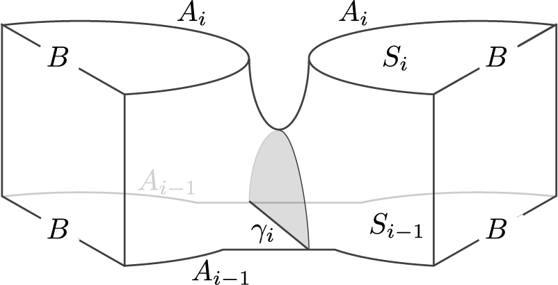
Figure 2.3 The elementary cobordism associated to cutting $S_{i-1}$
along
$S_{i-1}$
along $\gamma _i$
, shown before collapsing
$\gamma _i$
, shown before collapsing $B\times I$
.
$B\times I$
.
Concatenating these $M_i$
and gluing the final
$M_i$
and gluing the final $S_{2k}$
to the initial
$S_{2k}$
to the initial $S_0$
via h yields a manifold with boundary
$S_0$
via h yields a manifold with boundary $(B\times S^1) \cup V$
, where V is the (circular) union of the
$(B\times S^1) \cup V$
, where V is the (circular) union of the $V_i$
. The singular foliation on V has
$V_i$
. The singular foliation on V has $2k$
singular points associated to the transitions between topological types of the pages, while the regular leaves may be identified with curves of the form
$2k$
singular points associated to the transitions between topological types of the pages, while the regular leaves may be identified with curves of the form $A_i\times \{t\}$
. If
$A_i\times \{t\}$
. If $S_{i-1}\xrightarrow {{\textbf {add}}} S_{i}$
, then the corresponding hyperbolic point
$S_{i-1}\xrightarrow {{\textbf {add}}} S_{i}$
, then the corresponding hyperbolic point $h_i$
is negative; otherwise, it is positive. We denote the set of hyperbolic points with respect to this partition
$h_i$
is negative; otherwise, it is positive. We denote the set of hyperbolic points with respect to this partition $H=H_+\cup H_-$
. The signs match the partition of
$H=H_+\cup H_-$
. The signs match the partition of $[2k]$
introduced after Definition 2.4. Collapsing the components
$[2k]$
introduced after Definition 2.4. Collapsing the components $B\times S^1$
to a single copy of B yields a manifold with foliated boundary
$B\times S^1$
to a single copy of B yields a manifold with foliated boundary $(M, \partial M, \mathcal {F})$
. (See Definition 2.9, below, for a precise definition of this term.) Each endpoint of B labeled
$(M, \partial M, \mathcal {F})$
. (See Definition 2.9, below, for a precise definition of this term.) Each endpoint of B labeled $e_+$
becomes a positive elliptic point of the foliation, which we again denote by
$e_+$
becomes a positive elliptic point of the foliation, which we again denote by $e_+$
; likewise, an endpoint
$e_+$
; likewise, an endpoint $e_-$
becomes a negative elliptic point
$e_-$
becomes a negative elliptic point $e_-$
.
$e_-$
.
Example 2.8. We return to the foliated open book introduced in the first example. The associated smooth manifold is the solid torus shown in Figure 2.4. The images of $A_1$
and
$A_1$
and $A_2$
are shown in green and blue, respectively, on both the manifold on the left and in the associated boundary foliation on the right.
$A_2$
are shown in green and blue, respectively, on both the manifold on the left and in the associated boundary foliation on the right.

Figure 2.4 The smooth manifold (a solid torus) associated to the foliated open book from Figure 2.1 together with the foliation $\mathcal {F}$
on
$\mathcal {F}$
on $\partial M$
.
$\partial M$
.
In order to define the compatibility between contact structures and foliated open books, we examine the boundary foliation $\mathcal {F}$
more closely. To any smooth manifold constructed as above, we may associate an
$\mathcal {F}$
more closely. To any smooth manifold constructed as above, we may associate an $S^1$
-valued Morse function
$S^1$
-valued Morse function $\pi \colon M \setminus B \rightarrow S^1$
whose level sets are the pages of the open book and which restricts to the boundary as an
$\pi \colon M \setminus B \rightarrow S^1$
whose level sets are the pages of the open book and which restricts to the boundary as an $S^1$
-valued Morse function
$S^1$
-valued Morse function ${\widetilde {\pi }}:=\pi |_{\partial M}\colon \partial M\setminus E\to S^1$
with the same critical points as
${\widetilde {\pi }}:=\pi |_{\partial M}\colon \partial M\setminus E\to S^1$
with the same critical points as $\pi $
. The function
$\pi $
. The function $\pi $
has only index 1 and 2 critical points, and all of these are index 1 critical points for
$\pi $
has only index 1 and 2 critical points, and all of these are index 1 critical points for ${\widetilde {\pi }}$
. The index with respect to
${\widetilde {\pi }}$
. The index with respect to $\pi $
is visible in the sign of these hyperbolic points: index 2 critical points of
$\pi $
is visible in the sign of these hyperbolic points: index 2 critical points of $\pi $
give positive hyperbolic points of the foliation, while index 1 critical points of
$\pi $
give positive hyperbolic points of the foliation, while index 1 critical points of $\pi $
give negative hyperbolic points of the foliation. Heuristically, this means that the interesting features of
$\pi $
give negative hyperbolic points of the foliation. Heuristically, this means that the interesting features of $\pi $
may all be seen from the foliation on the boundary. One may build a signed singular foliation simply by patching together the local models of Figure 2.2, but in the context of this paper we will only encounter ordered signed singular foliations; equivalently, these are signed singular foliations that can be induced by an
$\pi $
may all be seen from the foliation on the boundary. One may build a signed singular foliation simply by patching together the local models of Figure 2.2, but in the context of this paper we will only encounter ordered signed singular foliations; equivalently, these are signed singular foliations that can be induced by an $S^1$
-valued Morse function. We therefore consider the map
$S^1$
-valued Morse function. We therefore consider the map ${\widetilde {\pi }}$
to be an essential part of the data and we write
${\widetilde {\pi }}$
to be an essential part of the data and we write $\mathcal {F}=({\widetilde {\pi }}, H=H_-\cup H_+, E=E_-\cup E_+)$
. We may also assume that
$\mathcal {F}=({\widetilde {\pi }}, H=H_-\cup H_+, E=E_-\cup E_+)$
. We may also assume that $0$
is a regular value of
$0$
is a regular value of ${\widetilde {\pi }}$
, and we further require that
${\widetilde {\pi }}$
, and we further require that ${\widetilde {\pi }}=\pm \phi $
on an
${\widetilde {\pi }}=\pm \phi $
on an $(r, \phi )$
-disk neighborhood of each elliptic point
$(r, \phi )$
-disk neighborhood of each elliptic point $e\in E$
, where the sign depends on the sign of the elliptic point. Here,
$e\in E$
, where the sign depends on the sign of the elliptic point. Here, $(r,\phi )$
is the standard polar coordinate system on
$(r,\phi )$
is the standard polar coordinate system on $D^2$
. By construction, the foliation on a manifold constructed from an abstract foliated open book has only elliptic and four-pronged hyperbolic singularities, with signs inherited from the partitions of E and H.
$D^2$
. By construction, the foliation on a manifold constructed from an abstract foliated open book has only elliptic and four-pronged hyperbolic singularities, with signs inherited from the partitions of E and H.
Definition 2.9. A manifold with foliated boundary is a compact oriented three-manifold equipped with an ordered signed singular foliation $\mathcal {F}=({\widetilde {\pi }}, H=H_-\cup H_+, E=E_-\cup E_+)$
on its boundary. We denote this collection of data by
$\mathcal {F}=({\widetilde {\pi }}, H=H_-\cup H_+, E=E_-\cup E_+)$
on its boundary. We denote this collection of data by $(M, \partial M, \mathcal {F})$
.
$(M, \partial M, \mathcal {F})$
.
We recall that these data include the $S^1$
-valued Morse function
$S^1$
-valued Morse function ${\widetilde {\pi }}$
, and we require that a diffeomorphism
${\widetilde {\pi }}$
, and we require that a diffeomorphism $f:(M_1, \partial M_1, \mathcal {F}_1) \rightarrow (M_2, \partial M_2, \mathcal {F}_2)$
between manifolds with foliated boundary must satisfy
$f:(M_1, \partial M_1, \mathcal {F}_1) \rightarrow (M_2, \partial M_2, \mathcal {F}_2)$
between manifolds with foliated boundary must satisfy ${\widetilde {\pi }}_2\circ f= {\widetilde {\pi }}_1$
.
${\widetilde {\pi }}_2\circ f= {\widetilde {\pi }}_1$
.
We have seen that an abstract foliated open book gives rise to a diffeomorphism class of manifolds with foliated boundary; we say a manifold with foliated boundary is compatible with $(\{S_i\}, h)$
if it is diffeomorphic to an output of this construction. A fixed manifold with foliated boundary will admit many different functions
$(\{S_i\}, h)$
if it is diffeomorphic to an output of this construction. A fixed manifold with foliated boundary will admit many different functions $\pi $
extending the Morse function
$\pi $
extending the Morse function ${\widetilde {\pi }}$
on the boundary, but compatibility identifies an equivalence class of such functions whose level sets are diffeomorphic to the pages
${\widetilde {\pi }}$
on the boundary, but compatibility identifies an equivalence class of such functions whose level sets are diffeomorphic to the pages $\{S_i\}$
.
$\{S_i\}$
.
Definition 2.10. Suppose that $\mathcal {F}=({\widetilde {\pi }}, H=H_-\cup H_+, E=E_-\cup E_+)$
is a signed singular foliation with no
$\mathcal {F}=({\widetilde {\pi }}, H=H_-\cup H_+, E=E_-\cup E_+)$
is a signed singular foliation with no $S^1$
leaves. We define
$S^1$
leaves. We define $R_+(\mathcal {F})$
to be a closed neighborhood of the union of the stable separatrices of hyperbolic points in
$R_+(\mathcal {F})$
to be a closed neighborhood of the union of the stable separatrices of hyperbolic points in $H_+$
, and let
$H_+$
, and let $R_-(\mathcal {F})=\overline {M\setminus R_+(\mathcal {F})}$
. The dividing curve
$R_-(\mathcal {F})=\overline {M\setminus R_+(\mathcal {F})}$
. The dividing curve $\Gamma (\mathcal {F})$
of
$\Gamma (\mathcal {F})$
of $\mathcal {F}$
is
$\mathcal {F}$
is $\partial R_+(\mathcal {F})=-\partial R_-(\mathcal {F})$
.
$\partial R_+(\mathcal {F})=-\partial R_-(\mathcal {F})$
.
Note that the serifed symbol $\Gamma $
used here is distinct from the sans-serif symbol
$\Gamma $
used here is distinct from the sans-serif symbol $\mathsf {\Gamma }$
introduced in Section 2.2.2 as part of the defining data of a bordered sutured manifold. The above construction of
$\mathsf {\Gamma }$
introduced in Section 2.2.2 as part of the defining data of a bordered sutured manifold. The above construction of $\Gamma (\mathcal {F})$
follows the construction of Giroux [Reference GirouxGir00] for dividing curves of characteristic foliations of convex surfaces and in our case too
$\Gamma (\mathcal {F})$
follows the construction of Giroux [Reference GirouxGir00] for dividing curves of characteristic foliations of convex surfaces and in our case too $\Gamma (\mathcal {F})$
indeed divides
$\Gamma (\mathcal {F})$
indeed divides $\mathcal {F}$
:
$\mathcal {F}$
: $\Gamma (\mathcal {F})$
is positively transverse to the leaves of
$\Gamma (\mathcal {F})$
is positively transverse to the leaves of $\mathcal {F}$
and it separates
$\mathcal {F}$
and it separates $\partial M\setminus \Gamma (\mathcal {F})$
into two parts, one of which contains all the positive singular points, while the other part contains all the negative singular points.Footnote
4
These properties in fact specify
$\partial M\setminus \Gamma (\mathcal {F})$
into two parts, one of which contains all the positive singular points, while the other part contains all the negative singular points.Footnote
4
These properties in fact specify $\Gamma (\mathcal {F})$
up to isotopy transverse to
$\Gamma (\mathcal {F})$
up to isotopy transverse to $\mathcal {F}$
, and we will often work with its equivalence class, only specifying the representative when needed. The choice of the representative then changes
$\mathcal {F}$
, and we will often work with its equivalence class, only specifying the representative when needed. The choice of the representative then changes $R_+(\mathcal {F})$
and
$R_+(\mathcal {F})$
and $R_-(\mathcal {F})$
accordingly, while still preserving the condition that
$R_-(\mathcal {F})$
accordingly, while still preserving the condition that $\Gamma (\mathcal {F})=\partial R_+(\mathcal {F})=-\partial R_-(\mathcal {F})$
. Note that distinct foliations on
$\Gamma (\mathcal {F})=\partial R_+(\mathcal {F})=-\partial R_-(\mathcal {F})$
. Note that distinct foliations on $\partial M$
may induce isotopic dividing sets; see Figure 2.5.
$\partial M$
may induce isotopic dividing sets; see Figure 2.5.

Figure 2.5 Left: A foliation on $S^2$
with four elliptic points and two hyperbolic points. Right: A foliation on
$S^2$
with four elliptic points and two hyperbolic points. Right: A foliation on $S^2$
with two elliptic points. The dividing set for each foliation is a circle.
$S^2$
with two elliptic points. The dividing set for each foliation is a circle.
Definition 2.11. Two ordered signed singular foliations $\mathcal {F}_1$
and
$\mathcal {F}_1$
and $\mathcal {F}_2$
on a surface
$\mathcal {F}_2$
on a surface $\Sigma $
are strongly topologically conjugate if there is an isotopy taking
$\Sigma $
are strongly topologically conjugate if there is an isotopy taking $\mathcal {F}_1$
to
$\mathcal {F}_1$
to $\mathcal {F}_2$
which respects the cyclic orders on the hyperbolic points.
$\mathcal {F}_2$
which respects the cyclic orders on the hyperbolic points.
The term ‘topological’ refers to the fact that the above isotopy may not be smooth. In fact, in the next definition, the isotopy cannot be chosen to be smooth.
Definition 2.12. [Reference Licata and VértesiLV20, Definition 3.8, 3.10] A contact structure $\xi _0$
on a manifold with foliated boundary
$\xi _0$
on a manifold with foliated boundary $(M, \partial M, \mathcal {F})$
is strictly supported by the abstract foliated open book
$(M, \partial M, \mathcal {F})$
is strictly supported by the abstract foliated open book $(\{S_i\}, h)$
if there is a diffeomorphism
$(\{S_i\}, h)$
if there is a diffeomorphism $f\colon (M', \partial M', \mathcal {F'})\to (M, \partial M, \mathcal {F})$
, where
$f\colon (M', \partial M', \mathcal {F'})\to (M, \partial M, \mathcal {F})$
, where $(M', \partial M', \mathcal {F'})$
is a manifold constructed from
$(M', \partial M', \mathcal {F'})$
is a manifold constructed from $(\{S_i\}, h)$
as above such that the pullback
$(\{S_i\}, h)$
as above such that the pullback $f^{\ast }\xi $
is the kernel of some contact one-form
$f^{\ast }\xi $
is the kernel of some contact one-form $\alpha $
on
$\alpha $
on $M'$
satisfying the following conditions:
$M'$
satisfying the following conditions:
-
1.
$\alpha (TB)>0$
; -
2. for all t,
$d\alpha |_{\pi ^{-1}(t)}$
is an area form; and -
3. for each pair of consecutive hyperbolic points at times
$t_1$
and
$t_2$
, there is a time
$t_*$
such that
$t_1<t_*<t_2$
with the property that the regular leaf
${\widetilde {\pi }}^{-1}(t_*)$
of
$\mathcal {F}$
is Legendrian.


A contact structure $\xi _1$
is supported by
$\xi _1$
is supported by $(\{S_i\}, h)$
if there exists a path of contact structures
$(\{S_i\}, h)$
if there exists a path of contact structures $\xi _t$
such that
$\xi _t$
such that $\xi _0$
is strictly supported by
$\xi _0$
is strictly supported by $(\{S_i\}, h)$
and for all t, the characteristic foliation
$(\{S_i\}, h)$
and for all t, the characteristic foliation $\mathcal {F}_{\xi _t}$
is strongly topologically conjugate to the characteristic foliation
$\mathcal {F}_{\xi _t}$
is strongly topologically conjugate to the characteristic foliation $\mathcal {F}_{\xi _0}$
.
$\mathcal {F}_{\xi _0}$
.
Definition 2.13. A foliated contact three-manifold $(M, \xi , \mathcal {F})$
is a manifold with foliated boundary together with a contact structure
$(M, \xi , \mathcal {F})$
is a manifold with foliated boundary together with a contact structure $\xi $
on M such that
$\xi $
on M such that $\mathcal {F}$
is strongly topologically conjugate to
$\mathcal {F}$
is strongly topologically conjugate to $\mathcal {F}_{\xi }$
.
$\mathcal {F}_{\xi }$
.
Theorem 2.14. [Reference Licata and VértesiLV20, Theorems 3.12, 7.1, 7.2] Any foliated open book with circle-free boundary foliation supports a unique isotopy class of contact structures, and any foliated contact three-manifold $(M,\xi ,\mathcal {F})$
admits a supporting foliated open book.
$(M,\xi ,\mathcal {F})$
admits a supporting foliated open book.
Remark 2.15. Because the signed singular foliation $\mathcal {F}$
data include a function
$\mathcal {F}$
data include a function $\widetilde {\pi }$
, a foliated contact three-manifold has a distinguished
$\widetilde {\pi }$
, a foliated contact three-manifold has a distinguished $t=0$
leaf, which we always assume to be regular.
$t=0$
leaf, which we always assume to be regular.
Distinct foliations may induce isotopic dividing sets, as illustrated in the following example.
Example 2.16. Let $(B^3, \xi _1, \mathcal {F}_1)$
and
$(B^3, \xi _1, \mathcal {F}_1)$
and $(B^3, \xi _2, \mathcal {F}_2)$
be two foliated contact three-balls with
$(B^3, \xi _2, \mathcal {F}_2)$
be two foliated contact three-balls with $\xi _1$
and
$\xi _1$
and $\xi _2$
tight, and with the foliations
$\xi _2$
tight, and with the foliations $\mathcal {F}_1$
and
$\mathcal {F}_1$
and $\mathcal {F}_2$
on the boundaries as in Figure 2.5. The two three-balls are equivalent in the sense that there is a contact embedding of one into the other with the property that the image of the embedded boundary is convexly isotopic to the boundary of the target manifold. This notion is an equivalence relation on contact manifolds with boundary, yet the given balls are distinct as foliated contact manifolds.
$\mathcal {F}_2$
on the boundaries as in Figure 2.5. The two three-balls are equivalent in the sense that there is a contact embedding of one into the other with the property that the image of the embedded boundary is convexly isotopic to the boundary of the target manifold. This notion is an equivalence relation on contact manifolds with boundary, yet the given balls are distinct as foliated contact manifolds.
2.3.2 Stabilization
Although each foliated open book supports a unique isotopy class of contact structures, there are many foliated open books which support the same class. Next, we define an operation which changes a foliated open book while preserving the contactomorphism class of the associated contact manifold.
Definition 2.17. Let $\gamma \subset S_0$
be a properly embedded arc with
$\gamma \subset S_0$
be a properly embedded arc with $\partial \gamma \subset B$
. The stabilization of
$\partial \gamma \subset B$
. The stabilization of $(\{S_i\}, h)$
along
$(\{S_i\}, h)$
along $\gamma $
is the foliated open book
$\gamma $
is the foliated open book $(\{S^{\prime }_i\}, h')$
defined as follows:
$(\{S^{\prime }_i\}, h')$
defined as follows:
-
•
$S_i'=S_i\cup H$
, where H is a one-handle attached along
$\partial \gamma $
; and -
•
$h'=\tau \circ \overline {h}$
, where
$\tau $
is a positive Dehn twist along the circle formed by
$\gamma $
and the core of H. (Here,
$\overline {h}$
denotes the extension of h to H by the identity.)


In order to define stabilization along some arc in a page besides $S_0$
, we first describe an operation on foliated open books which preserves the contactomorphism type of the associated manifold.
$S_0$
, we first describe an operation on foliated open books which preserves the contactomorphism type of the associated manifold.
Definition 2.18. [Reference Licata and VértesiLV20, Definition 3.16] The $1$
-shift of an abstract foliated open book
$1$
-shift of an abstract foliated open book $(\{S_i\}_{i=0}^{2k},h)$
is the foliated open book
$(\{S_i\}_{i=0}^{2k},h)$
is the foliated open book
 $$\begin{align*}(\{S_i[1]\}_{i=0}^{2k},h[1])=(\{S_1,S_2,\dots,S_{2k},S_1'\},h'),\end{align*}$$
where
-
- if
$S_{0}\xrightarrow [\gamma _{1}]{{\textbf {cut}}} S_1$
, then
$S_1'$
is defined by the relation
$S_{2k}\xrightarrow [{h^{-1}(\gamma _{1})}]{{\textbf {cut}}} S_1'$
and
$h'$
is the restriction of h to
$S_1'$
; -
- if
$S_{0}\xrightarrow [{p_0, q_0}]{{\textbf {add}}} S_1$
, then
$S_1'$
is defined by the relation
$S_{2k}\xrightarrow [{ h^{-1}(p_0), h^{-1}(q_0) }]{{\textbf {add}}} S_1'$
and
$h'$
is h extended by the identity on the added one-handle.


An r-fold iteration of the shift operation is called an r-shift and denoted by $(\{S_i[r]\}_{i=0}^{2k},h[r])$
. One can analogously define r-shifts for
$(\{S_i[r]\}_{i=0}^{2k},h[r])$
. One can analogously define r-shifts for $r<0$
.
$r<0$
.
Shifts correspond to postcomposing $\pi $
with a diffeomorphism of
$\pi $
with a diffeomorphism of $S^1$
.
$S^1$
.
Definition 2.19. Let $\gamma \subset S_r$
be a properly embedded arc with
$\gamma \subset S_r$
be a properly embedded arc with $\partial \gamma \subset B$
. The stabilization of
$\partial \gamma \subset B$
. The stabilization of $(\{S_i\}, h)$
along
$(\{S_i\}, h)$
along $\gamma \subset S_r$
is the foliated open book
$\gamma \subset S_r$
is the foliated open book $(\{S^{\prime }_i\}, h')$
defined as follows:
$(\{S^{\prime }_i\}, h')$
defined as follows:
-
1. first perform an r-shift of
$(\{S_i\},h)$
to
$(\{S_i[r]\},h[r])$
; -
2. stabilize as in Definition 2.17 along the image of
$\gamma \subset S_0[r]$
; -
3. perform a
$(-r)$
-shift to obtain
$(\{S_i'\},h')$
, where
$S_i'$
is still obtained from
$S_i$
by a handle attachment along p and q.


It is easy to see that stabilizing does not change the underlying manifold with foliated boundary.
Theorem 2.20. [Reference Licata and VértesiLV20, Proposition 6.8, Theorem 6.9] Let $(\{S_i\}, h)$
be a foliated open book and
$(\{S_i\}, h)$
be a foliated open book and $(\{S_i'\}, h')$
be a positive stabilization of
$(\{S_i'\}, h')$
be a positive stabilization of $(\{S_i\}, h)$
. Then the corresponding contact three-manifolds are contactomorphic. Furthermore, if two foliated open books support contactomorphic foliated contact three-manifolds, then they admit a common positive stabilization.
$(\{S_i\}, h)$
. Then the corresponding contact three-manifolds are contactomorphic. Furthermore, if two foliated open books support contactomorphic foliated contact three-manifolds, then they admit a common positive stabilization.
2.3.3 Sorted foliated open books
Next, we introduce some additional bookkeeping to record the cutting arcs and cocore arcs on all possible pages of the foliated open book. This additional information corresponds to a choice of a gradient-like vector field for $\pi $
on the associated smooth manifold, as we will describe in Section 2.3.4.
$\pi $
on the associated smooth manifold, as we will describe in Section 2.3.4.
If $S_{{i-1}}\xrightarrow {{\textbf {add}}} S_{i}$
, then for all
$S_{{i-1}}\xrightarrow {{\textbf {add}}} S_{i}$
, then for all $j\geq {i}$
, decorate
$j\geq {i}$
, decorate $S_{j}$
with a cocore of the added handle and label this cocore
$S_{j}$
with a cocore of the added handle and label this cocore $\gamma _i^-$
. If
$\gamma _i^-$
. If $S_{{i-1}}\xrightarrow {{\textbf {cut}}} S_{i}$
along
$S_{{i-1}}\xrightarrow {{\textbf {cut}}} S_{i}$
along $\gamma \subset S_{{i-1}}$
, then for all
$\gamma \subset S_{{i-1}}$
, then for all $j\leq {i-1}$
, decorate
$j\leq {i-1}$
, decorate $S_j$
with the cutting curve and label it
$S_j$
with the cutting curve and label it $\gamma _i^+$
.
$\gamma _i^+$
.
We call the $\gamma _i^\pm $
sorting arcs. Note that by an abuse of notation we use a single label
$\gamma _i^\pm $
sorting arcs. Note that by an abuse of notation we use a single label $\gamma _i^\pm $
to refer to distinct copies of the sorting arcs on multiple
$\gamma _i^\pm $
to refer to distinct copies of the sorting arcs on multiple $S_j$
. In general, sorting arcs may intersect (and consequently some sorting arcs may appear as a union of disconnected intervals on some pages). We will shortly restrict to the subclass of sorted foliated open books [Reference Licata and VértesiLV20, Section 5.3], which are characterized by the requirement that the sorting arcs are disjoint on all pages, together with a prescribed ordering of the intersections between sorting arcs and regular leaves. In the sorted case, we enhance the notation for describing a foliated open book to reflect these additional choices.
$S_j$
. In general, sorting arcs may intersect (and consequently some sorting arcs may appear as a union of disconnected intervals on some pages). We will shortly restrict to the subclass of sorted foliated open books [Reference Licata and VértesiLV20, Section 5.3], which are characterized by the requirement that the sorting arcs are disjoint on all pages, together with a prescribed ordering of the intersections between sorting arcs and regular leaves. In the sorted case, we enhance the notation for describing a foliated open book to reflect these additional choices.
Definition 2.21. An abstract foliated open book $(\{S_i\}, h, \{\gamma _i^\pm \})$
is sorted if the following properties hold:
$(\{S_i\}, h, \{\gamma _i^\pm \})$
is sorted if the following properties hold:
-
1. On each page
$S_i$
and for each component I of
$A_i$
with
$\partial I=\{e_+, e_-\}$
, there exist disjoint subintervals
$I_+$
and
$I_-$
such that
$I_+$
contains
$e_+\cup \bigcup _j \big (\gamma ^+_j\cap I\big )$
and
$I_{-}$
contains
$e_-\cup \bigcup _j \big (\gamma ^-_j\cap I\big )$
. -
2. For
$i {<} j< l$
, on each component of
$A_i$
any endpoint of
$\gamma _l^+$
is closer to
$e_+$
than any endpoint of
$\gamma _j^+ $
; -
3. For
$j<l\leq i$
, on each component of
$A_i$
any endpoint of
$\gamma _l^-$
lies closer to
$e_+$
than any endpoint of
$\gamma _j^-$
; -
4. On each page, the sorting arcs are connected, properly embedded, and disjoint.


See Figure 2.7 in Example 2.24 for an illustration of the ordering conventions given above. Sorted foliated open books are useful because of their close relation to partial open books, which will be described in Section 2.3.5. Below, we show that a foliated open book need not be sorted.
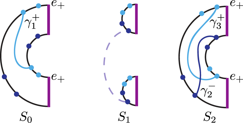
Figure 2.6 The first three pages of the foliated open book from Example 2.5.

Figure 2.7 The stabilization arc $\gamma \subset S_0$
is chosen to have one endpoint on each interval of the binding B so that it crosses each of of the intersecting sorting arcs in Figure 2.6 exactly once. There is a right-handed Dehn twist identifying the two copies of the
$\gamma \subset S_0$
is chosen to have one endpoint on each interval of the binding B so that it crosses each of of the intersecting sorting arcs in Figure 2.6 exactly once. There is a right-handed Dehn twist identifying the two copies of the $S_2'$
page, while the monodromy
$S_2'$
page, while the monodromy $h' \colon \thinspace S_4'\to S_0'$
is translation in the plane of the page. The sorting arcs
$h' \colon \thinspace S_4'\to S_0'$
is translation in the plane of the page. The sorting arcs $\gamma ^+$
are shown in light blue, and the sorting arcs
$\gamma ^+$
are shown in light blue, and the sorting arcs $\gamma ^-$
are shown in dark blue. Subintervals
$\gamma ^-$
are shown in dark blue. Subintervals $I_\pm \subset A_0$
are highlighted in green and orange on
$I_\pm \subset A_0$
are highlighted in green and orange on $S_0$
and may be chosen analogously on the other pages.
$S_0$
and may be chosen analogously on the other pages.
Example 2.22. The foliated open book from Example 2.5 is not sorted. To see this, we start on the $S_0$
page and attempt to decorate each successive page with cutting arcs which realize the topological transitions between pages and whose endpoints also satisfy the ordering conditions of Definition 2.21.
$S_0$
page and attempt to decorate each successive page with cutting arcs which realize the topological transitions between pages and whose endpoints also satisfy the ordering conditions of Definition 2.21.
Cutting along $\gamma _1^+$
on
$\gamma _1^+$
on $S_0$
yields
$S_0$
yields $S_1$
, while attaching a handle to
$S_1$
, while attaching a handle to $S_1$
gives rise to
$S_1$
gives rise to $S_2$
, which is decorated with the new cocore
$S_2$
, which is decorated with the new cocore $\gamma _2^-$
. However, any cutting arc associated to
$\gamma _2^-$
. However, any cutting arc associated to $h_3$
necessarily intersects
$h_3$
necessarily intersects $\gamma _2^-$
on
$\gamma _2^-$
on $S_2$
, as the endpoints of
$S_2$
, as the endpoints of $\gamma _3^+$
must lie closer to the positive ends of
$\gamma _3^+$
must lie closer to the positive ends of $A_2$
than the endpoints of
$A_2$
than the endpoints of $\gamma _2^-$
. Thus, the foliated open book is not sorted. See Figure 2.6.
$\gamma _2^-$
. Thus, the foliated open book is not sorted. See Figure 2.6.
We may always stabilize a foliated open book to obtain a sorted one.
Theorem 2.23. Any foliated contact three-manifold $(M,\xi ,\mathcal {F})$
admits a supporting sorted foliated open book. If two sorted foliated open books support the same foliated contact three-manifold, then we can stabilize each through sorted foliated open books to obtain a common sorted foliated open book. Moreover, all of these stabilizations can be assumed to be performed on the
$(M,\xi ,\mathcal {F})$
admits a supporting sorted foliated open book. If two sorted foliated open books support the same foliated contact three-manifold, then we can stabilize each through sorted foliated open books to obtain a common sorted foliated open book. Moreover, all of these stabilizations can be assumed to be performed on the $S_0$
page as in Definition 2.17.
$S_0$
page as in Definition 2.17.
Proof. The first two statements are taken from [Reference Licata and VértesiLV20, Theorem 3.12, Proposition 8.4, Theorem 8.14]. The final claim that the necessary stabilizations may be assumed to occur on the $S_0$
page is implicit in [Reference Licata and VértesiLV20], as explained next; we include the brief argument here, although it relies on the connection between foliated and partial open books described in Section 2.3.5. Specifically, the proof of [Reference Licata and VértesiLV20, Proposition 8.6] explains why stabilizations on the
$S_0$
page is implicit in [Reference Licata and VértesiLV20], as explained next; we include the brief argument here, although it relies on the connection between foliated and partial open books described in Section 2.3.5. Specifically, the proof of [Reference Licata and VértesiLV20, Proposition 8.6] explains why stabilizations on the $S_0$
page suffice to turn an arbitrary sorted foliated open book into a sufficiently stabilizedFootnote
5
foliated open book. The proof that two sufficiently stabilized open books admit a common stabilization relies on Giroux correspondence for the associated partial open books and, hence, leads again to stabilizations on
$S_0$
page suffice to turn an arbitrary sorted foliated open book into a sufficiently stabilizedFootnote
5
foliated open book. The proof that two sufficiently stabilized open books admit a common stabilization relies on Giroux correspondence for the associated partial open books and, hence, leads again to stabilizations on $S_0$
.
$S_0$
.
Example 2.24. Figure 2.7 shows that the foliated open book from Example 2.5 may be stabilized to a sorted foliated open book. Starting from index $S_0$
, the first obstruction to being sorted occurred as an intersection between
$S_0$
, the first obstruction to being sorted occurred as an intersection between $\gamma _2^-$
and
$\gamma _2^-$
and $\gamma _3^+$
on
$\gamma _3^+$
on $S_2$
. This intersection may be removed by stabilizing ‘at’ the
$S_2$
. This intersection may be removed by stabilizing ‘at’ the $S_2$
page; that is, by shifting twice and then stabilizing at the new
$S_2$
page; that is, by shifting twice and then stabilizing at the new $S_0$
. Each new page is obtained from the corresponding old page by attaching a one-handle with one attaching interval on each binding component. The new final maps to the new initial page by a positive Dehn twist; after shifting back, this becomes a positive Dehn twist identifying the two copies of the
$S_0$
. Each new page is obtained from the corresponding old page by attaching a one-handle with one attaching interval on each binding component. The new final maps to the new initial page by a positive Dehn twist; after shifting back, this becomes a positive Dehn twist identifying the two copies of the $S_2'$
page, as shown. Thus,
$S_2'$
page, as shown. Thus, $\gamma _2^-$
changes by a positive Dehn twist as it ascends to higher-index pages, while
$\gamma _2^-$
changes by a positive Dehn twist as it ascends to higher-index pages, while $\gamma _3^+$
changes by a negative Dehn twist as it descends to lower-index pages.
$\gamma _3^+$
changes by a negative Dehn twist as it descends to lower-index pages.
When depicting a sequence of pages, there is an implicit identification by translation in the page unless otherwise noted. In this example, the one nontranslation occurs at $S_2'$
while the map from
$S_2'$
while the map from $S^{\prime }_4$
to
$S^{\prime }_4$
to $S_0'$
remains translation in the plane of the page, as seen on Figure 2.7. The result is a sorted foliated open book for the original contact manifold with foliated boundary.
$S_0'$
remains translation in the plane of the page, as seen on Figure 2.7. The result is a sorted foliated open book for the original contact manifold with foliated boundary.
2.3.4 Gradient flows on foliated open books
As in Section 2.3.1, we consider the smooth manifold with foliated boundary $(M, \partial M, \mathcal {F})$
constructed from a foliated open book. The initial abstract data determines an equivalence class of circle-valued Morse functions
$(M, \partial M, \mathcal {F})$
constructed from a foliated open book. The initial abstract data determines an equivalence class of circle-valued Morse functions $\pi \colon \thinspace M\setminus B\rightarrow S^1$
[Reference Licata and VértesiLV20, Section 5.2]. The level sets of
$\pi \colon \thinspace M\setminus B\rightarrow S^1$
[Reference Licata and VértesiLV20, Section 5.2]. The level sets of $\pi $
are the pages, and the restriction
$\pi $
are the pages, and the restriction ${\widetilde {\pi }} \colon \thinspace \partial M\setminus B \rightarrow S^1$
is again a circle-valued Morse function with the same set of critical points. In this setting, one may consider the critical submanifolds of a gradient-like vector field for
${\widetilde {\pi }} \colon \thinspace \partial M\setminus B \rightarrow S^1$
is again a circle-valued Morse function with the same set of critical points. In this setting, one may consider the critical submanifolds of a gradient-like vector field for $\pi $
parallel to
$\pi $
parallel to $\partial M$
, which thus restricts to a gradient-like vector field for
$\partial M$
, which thus restricts to a gradient-like vector field for ${\widetilde {\pi }}$
. The intersection of the critical submanifolds with the regular level sets of
${\widetilde {\pi }}$
. The intersection of the critical submanifolds with the regular level sets of $\pi $
determines sorting arcs on the pages of the corresponding abstract foliated open book [Reference Licata and VértesiLV20, Section 5.3]. Thus, a foliated open book is sorted when a gradient-like vector field on
$\pi $
determines sorting arcs on the pages of the corresponding abstract foliated open book [Reference Licata and VértesiLV20, Section 5.3]. Thus, a foliated open book is sorted when a gradient-like vector field on $\partial M$
that satisfies the ordering conditions for sorting arcs extends to a gradient-like vector field on M whose critical submanifolds are disjoint.
$\partial M$
that satisfies the ordering conditions for sorting arcs extends to a gradient-like vector field on M whose critical submanifolds are disjoint.
Any surface with an open book foliation decomposes along regular leaves into square tiles that each contain precisely one hyperbolic singularity. Figure 2.8 shows the flowlines of a preferred $\nabla {\widetilde {\pi }}$
on such a tile; these flowlines satisfy the ordering conditions in Definition 2.21, although ensuring their extension to M yields a sorted foliated open book may require stabilization.
$\nabla {\widetilde {\pi }}$
on such a tile; these flowlines satisfy the ordering conditions in Definition 2.21, although ensuring their extension to M yields a sorted foliated open book may require stabilization.

Figure 2.8 The tile of $\mathcal {F}$
shows purple flowlines of
$\mathcal {F}$
shows purple flowlines of $\nabla {\widetilde {\pi }}$
which satisfy the sorted ordering conditions.
$\nabla {\widetilde {\pi }}$
which satisfy the sorted ordering conditions.
The Morse perspective is useful not only for building geometric intuition but also for relating the boundary decorations to those in the interior of the manifold. For example, a sorting arc $\gamma ^{+}_i$
is isotopic through the associated stable critical submanifold of
$\gamma ^{+}_i$
is isotopic through the associated stable critical submanifold of $\nabla \pi $
to the stable submanifold of
$\nabla \pi $
to the stable submanifold of $\nabla {\widetilde {\pi }}$
on
$\nabla {\widetilde {\pi }}$
on $\partial M$
which passes through the corresponding positive hyperbolic point
$\partial M$
which passes through the corresponding positive hyperbolic point $h_i$
. Likewise, a sorting arc
$h_i$
. Likewise, a sorting arc $\gamma ^{-}_i$
is isotopic through the associated unstable critical submanifold of
$\gamma ^{-}_i$
is isotopic through the associated unstable critical submanifold of $\nabla \pi $
to the unstable submanifold of
$\nabla \pi $
to the unstable submanifold of $\nabla {\widetilde {\pi }}$
on
$\nabla {\widetilde {\pi }}$
on $\partial M$
which passes through the corresponding negative hyperbolic point
$\partial M$
which passes through the corresponding negative hyperbolic point $h_i$
. Conditions 1, 2 and 3 in Definition 2.21 are chosen so that the graphs formed by the (un)stable separatrices of positive (negative) hyperbolic points with respect to
$h_i$
. Conditions 1, 2 and 3 in Definition 2.21 are chosen so that the graphs formed by the (un)stable separatrices of positive (negative) hyperbolic points with respect to $\mathcal {F}$
and with respect to
$\mathcal {F}$
and with respect to $\nabla {\widetilde {\pi }}$
are isotopic. See [Reference Licata and VértesiLV20, Lemma 8.8]. In the next section, this will allow us to define certain subsurfaces as neighborhoods of either graph.
$\nabla {\widetilde {\pi }}$
are isotopic. See [Reference Licata and VértesiLV20, Lemma 8.8]. In the next section, this will allow us to define certain subsurfaces as neighborhoods of either graph.
2.3.5 Sufficiently stabilized foliated open books and the associated partial open book
Sorted foliated open books are closely related to partial open books, and [Reference Licata and VértesiLV20] introduced the technical designation of a ‘sufficiently stabilized’ foliated open book. In this section, we recall this definition and show that a sufficiently stabilized foliated open book naturally has a companion partial open book. Throughout this section, we will let $(\{S_i\}_{i=0}^{2k},h,\{\gamma _i^\pm \})$
be a sorted foliated open book and
$(\{S_i\}_{i=0}^{2k},h,\{\gamma _i^\pm \})$
be a sorted foliated open book and $(M, \xi , \mathcal {F})$
be the supported foliated contact three-manifold. We further assume that either
$(M, \xi , \mathcal {F})$
be the supported foliated contact three-manifold. We further assume that either $k>0$
or
$k>0$
or $|\partial M|>1$
; the only foliated open books this excludes are those formed from an honest open book by removing a neighborhood of a single point on the binding.
$|\partial M|>1$
; the only foliated open books this excludes are those formed from an honest open book by removing a neighborhood of a single point on the binding.
Set
 $$\begin{align*}R_i=N_{\lrcorner}\big(A_i \cup\big(\bigcup_{i < j}\gamma_j^+\big)\cup\big(\bigcup_{i\geq j}\gamma_j^-\big)\big) \subset S_i,\\[-17pt]\end{align*}$$
where $N_{\lrcorner }$
denotes a ‘cornered’ neighborhood of
$N_{\lrcorner }$
denotes a ‘cornered’ neighborhood of $A_i \cup (\bigcup _{i < j}\gamma _j^+)\cup (\bigcup _{i\geq j}\gamma _j^-)$
, with corners at E so that
$A_i \cup (\bigcup _{i < j}\gamma _j^+)\cup (\bigcup _{i\geq j}\gamma _j^-)$
, with corners at E so that $R_i$
meets B only at E. Furthermore, define
$R_i$
meets B only at E. Furthermore, define
 $$\begin{align*}P_i=\overline{S_i\setminus R_i},\end{align*}$$
as shown on the left in Figure 2.9. Since only the $R_i$
change with i, we can identify all the
$R_i$
change with i, we can identify all the $P_i$
with each other by the flow of the gradient-like vector field. We denote the composition of these identifications from
$P_i$
with each other by the flow of the gradient-like vector field. We denote the composition of these identifications from $P_0\subset S_0$
onto
$P_0\subset S_0$
onto $P_{2k}\subset S_{2k}$
by
$P_{2k}\subset S_{2k}$
by $\iota $
. Let
$\iota $
. Let $\widetilde {S}=S_{0}$
,
$\widetilde {S}=S_{0}$
, $\widetilde {P}=P_{0}$
and
$\widetilde {P}=P_{0}$
and $\tilde {h}=h\vert _{P_{2k}}\circ \iota $
.
$\tilde {h}=h\vert _{P_{2k}}\circ \iota $
.

Figure 2.9 The shaded regions show the cornered neighborhoods $R_i''$
in each page of the sufficiently stabilized open book. As in Example 2.24, successive pages are identified by translation except for the right-handed Dehn twist
$R_i''$
in each page of the sufficiently stabilized open book. As in Example 2.24, successive pages are identified by translation except for the right-handed Dehn twist $\tau $
at
$\tau $
at $S_2''$
.
$S_2''$
.
Definition 2.25. [Reference Licata and VértesiLV20, Proof of Proposition 8.6] The sorted foliated open book $(\{S_i\}_{i=0}^{2k}, h, \{\gamma _i\})$
is sufficiently stabilized if each component of
$(\{S_i\}_{i=0}^{2k}, h, \{\gamma _i\})$
is sufficiently stabilized if each component of $P_0$
intersects the boundary of
$P_0$
intersects the boundary of $R_0$
in at least two intervals.
$R_0$
in at least two intervals.
This condition ensures that $(\widetilde {S}, \widetilde {P}, \tilde {h})$
is a partial open book whose pages embed into the pages of
$(\widetilde {S}, \widetilde {P}, \tilde {h})$
is a partial open book whose pages embed into the pages of $(\{S_i\}_{i=0}^{2k}, h, \{\gamma _i\})$
. As the term suggests, this condition may always be achieved by a sequence of positive stabilizations, and in fact, these may be chosen to occur on the
$(\{S_i\}_{i=0}^{2k}, h, \{\gamma _i\})$
. As the term suggests, this condition may always be achieved by a sequence of positive stabilizations, and in fact, these may be chosen to occur on the $S_0$
page.
$S_0$
page.
Theorem 2.26. [Reference Licata and VértesiLV20, Proposition 8.10] With the notation above, the partial open book $(\widetilde {S},\widetilde {P},\widetilde {h})$
is compatible with a contact manifold
$(\widetilde {S},\widetilde {P},\widetilde {h})$
is compatible with a contact manifold $(\widetilde {M},\widetilde {\xi })$
which is contactomorphic to
$(\widetilde {M},\widetilde {\xi })$
which is contactomorphic to $(M,\xi )$
. Furthermore, under this contactomorphism, the image of the dividing set of the characteristic foliation of
$(M,\xi )$
. Furthermore, under this contactomorphism, the image of the dividing set of the characteristic foliation of $\xi $
on
$\xi $
on $\partial M$
divides
$\partial M$
divides $\widetilde {\mathcal {F}}$
.
$\widetilde {\mathcal {F}}$
.
Example 2.27. In this example, we return to the foliated open book of Example 2.24, which is not sufficiently stabilized. Recall that $R^{\prime }_0$
is constructed as a cornered neighborhood of the sorting arcs together with
$R^{\prime }_0$
is constructed as a cornered neighborhood of the sorting arcs together with $A^{\prime }_0$
. Observe that
$A^{\prime }_0$
. Observe that $P^{\prime }_0:=S_0'\setminus R_0'$
consists of two bigons, each with an edge on B and an edge on the annular
$P^{\prime }_0:=S_0'\setminus R_0'$
consists of two bigons, each with an edge on B and an edge on the annular $\partial R^{\prime }_0$
. It follows that
$\partial R^{\prime }_0$
. It follows that $S^{\prime }_0$
cannot be built up from
$S^{\prime }_0$
cannot be built up from $R^{\prime }_0$
by adding one-handles, which is the topological requirement for the surface/subsurface pair to define a partial open book.
$R^{\prime }_0$
by adding one-handles, which is the topological requirement for the surface/subsurface pair to define a partial open book.
Figure 2.9 shows a sufficiently stabilized foliated open book for the same manifold, built by stabilizing along the dotted arc which connected the two components of the binding. The new monodromy is the composition of the original monodromy with a positive Dehn twist along the circle formed by the core of the added handle and the stabilizing arc.
The new $P^{\prime \prime }_0:=S_0''\setminus R_0''$
is a single disk whose boundary intersects
$P^{\prime \prime }_0:=S_0''\setminus R_0''$
is a single disk whose boundary intersects $\partial R^{\prime \prime }_0$
along two intervals; this ensures that
$\partial R^{\prime \prime }_0$
along two intervals; this ensures that $(\widetilde {S}'', \widetilde {P}'', \widetilde {h}'')$
is a partial open book. In order to understand
$(\widetilde {S}'', \widetilde {P}'', \widetilde {h}'')$
is a partial open book. In order to understand $\widetilde {h}''$
, we first examine the flow of
$\widetilde {h}''$
, we first examine the flow of $P_0''$
through the manifold. Recall from Example 2.24 that the only nontrivial identification between successive pages is a right-handed Dehn twist at the
$P_0''$
through the manifold. Recall from Example 2.24 that the only nontrivial identification between successive pages is a right-handed Dehn twist at the $S_2''$
page before the cut yielding
$S_2''$
page before the cut yielding $S_3''$
. The twist is along the core of the annular
$S_3''$
. The twist is along the core of the annular $R_2''$
, so
$R_2''$
, so $P_4''$
is isotopic, relative to
$P_4''$
is isotopic, relative to $A_4''=A_0''$
, to
$A_4''=A_0''$
, to $P_0''$
. Thus, the partial open book monodromy is simply the restriction of the foliated open book monodromy to
$P_0''$
. Thus, the partial open book monodromy is simply the restriction of the foliated open book monodromy to $P_4''$
.
$P_4''$
.
As shown in [Reference Licata and VértesiLV20, Lemma 8.12], the cornered diffeomorphism type of the subsurfaces $R_i\subset S_i$
depends only on the foliation
$R_i\subset S_i$
depends only on the foliation $\mathcal {F}$
, rather than on the pages
$\mathcal {F}$
, rather than on the pages $S_i$
. Construct the corresponding contact three-manifold
$S_i$
. Construct the corresponding contact three-manifold $(M,\xi ,\mathcal {F})$
for a sorted abstract foliated open book
$(M,\xi ,\mathcal {F})$
for a sorted abstract foliated open book $(\{S_i\},h,\{\gamma _i^\pm \})$
. Recall from Definition 2.10 that the subsurface
$(\{S_i\},h,\{\gamma _i^\pm \})$
. Recall from Definition 2.10 that the subsurface $R_+(\mathcal {F})$
(respectively
$R_+(\mathcal {F})$
(respectively $R_-(\mathcal {F})$
) of
$R_-(\mathcal {F})$
) of $\partial M$
is a closed neighborhood of the (un)stable separatrices corresponding to positive (negative) hyperbolic points of
$\partial M$
is a closed neighborhood of the (un)stable separatrices corresponding to positive (negative) hyperbolic points of $\mathcal {F}$
.
$\mathcal {F}$
.
As noted in Section 2.3.4, the graph of positive separatrices of $\nabla {\widetilde {\pi }}$
from positive hyperbolic points on
$\nabla {\widetilde {\pi }}$
from positive hyperbolic points on $\partial M$
is (nonsmoothly) isotopic to the graph of positive separatrices of
$\partial M$
is (nonsmoothly) isotopic to the graph of positive separatrices of $\mathcal {F}$
from positive hyperbolic points on
$\mathcal {F}$
from positive hyperbolic points on $\partial M$
. On the other hand, the former is isotopic through the stable critical submanifolds to a neighborhood of the sorting arcs
$\partial M$
. On the other hand, the former is isotopic through the stable critical submanifolds to a neighborhood of the sorting arcs $\cup _{H_+}\gamma ^+_i$
on
$\cup _{H_+}\gamma ^+_i$
on $S_0$
. This yields an identification between
$S_0$
. This yields an identification between $R_+(\mathcal {F})\subset \partial M$
and
$R_+(\mathcal {F})\subset \partial M$
and $R_0\subset S_0$
. Similarly, studying negative separatrices of negative hyperbolic points and unstable critical submanifolds yields an identification between
$R_0\subset S_0$
. Similarly, studying negative separatrices of negative hyperbolic points and unstable critical submanifolds yields an identification between $R_-(\mathcal {F})\subset \partial M$
and
$R_-(\mathcal {F})\subset \partial M$
and $R_{2k}\subset S_{2k}$
.
$R_{2k}\subset S_{2k}$
.
Similarly, all the $R_i$
can be identified with surfaces described only using the foliation
$R_i$
can be identified with surfaces described only using the foliation $\mathcal {F}$
, independently of the foliated open book, as follows. Recall that
$\mathcal {F}$
, independently of the foliated open book, as follows. Recall that $R_i$
is the (cornered) neighborhood of the union of
$R_i$
is the (cornered) neighborhood of the union of $A_i$
and the intersection of all stable and unstable submanifolds of
$A_i$
and the intersection of all stable and unstable submanifolds of $\nabla \pi $
with
$\nabla \pi $
with $S_i$
. Each of these intersections can be pushed up (or down) onto
$S_i$
. Each of these intersections can be pushed up (or down) onto $\partial M$
along the corresponding stable (or unstable) submanifolds. While performing these isotopies we push the half-neighborhood of
$\partial M$
along the corresponding stable (or unstable) submanifolds. While performing these isotopies we push the half-neighborhood of $A_i$
up along
$A_i$
up along $I_+$
and down along
$I_+$
and down along $I_-$
; the surface obtained after the isotopy is not a submanifold of
$I_-$
; the surface obtained after the isotopy is not a submanifold of $\partial M$
, as it has a half twist in the middle of each component I of
$\partial M$
, as it has a half twist in the middle of each component I of $A_i$
which extends into the interior of M. See Figure 2.10.
$A_i$
which extends into the interior of M. See Figure 2.10.

Figure 2.10 The blue region on the left-hand picture is the cornered neighborhood $R_i\subset S_i$
. On the right-hand figure,
$R_i\subset S_i$
. On the right-hand figure, $R_i$
has been isotoped through M in the direction of the indicated arrows to lie mostly on
$R_i$
has been isotoped through M in the direction of the indicated arrows to lie mostly on $\partial M$
. The small arrow indicates the half twist which extends into the interior of M. Note that B has been blown up to
$\partial M$
. The small arrow indicates the half twist which extends into the interior of M. Note that B has been blown up to $B\times I$
for clarity.
$B\times I$
for clarity.
2.3.6 Gluing foliated open books
In order to glue foliated open books, we describe the matching conditions imposed upon their boundary foliations. Recall that a foliation $\mathcal {F}$
on a surface F always refers to the data of a signed foliation together with the function
$\mathcal {F}$
on a surface F always refers to the data of a signed foliation together with the function ${\widetilde {\pi }}\colon F\setminus E\to S^1$
whose level sets are the leaves of
${\widetilde {\pi }}\colon F\setminus E\to S^1$
whose level sets are the leaves of $\mathcal {F}$
.
$\mathcal {F}$
.
Definition 2.28. The reverse of a foliation $\mathcal {F}$
on F is the foliation on
$\mathcal {F}$
on F is the foliation on $-F$
which is equal to
$-F$
which is equal to $\mathcal {F}$
pointwise but with the leaf orientations and signs of singular points reversed.
$\mathcal {F}$
pointwise but with the leaf orientations and signs of singular points reversed.
The main advantage of foliated open books is that they are well suited for gluing. Suppose that $(M^L,\xi ^L,\mathcal {F}^L)$
and
$(M^L,\xi ^L,\mathcal {F}^L)$
and $(M^R,\xi ^R,\mathcal {F}^R)$
are foliated contact three-manifolds such that there exists an orientation-reversing diffeomorphism
$(M^R,\xi ^R,\mathcal {F}^R)$
are foliated contact three-manifolds such that there exists an orientation-reversing diffeomorphism $\psi \colon \partial M^L \to \partial M^R$
that maps the reverse of the foliation
$\psi \colon \partial M^L \to \partial M^R$
that maps the reverse of the foliation $\mathcal {F}^L$
onto
$\mathcal {F}^L$
onto $\mathcal {F}^R$
.
$\mathcal {F}^R$
.
Recall that by hypothesis, the boundary foliations are divided, so the boundaries $\partial M^{\bullet }$
are convex with respect to
$\partial M^{\bullet }$
are convex with respect to $\xi ^{\bullet }$
. (Here, and throughout this section,
$\xi ^{\bullet }$
. (Here, and throughout this section, $\bullet $
will be an element of the set
$\bullet $
will be an element of the set $\{R, L\}$
.) Since the contact structures are I-invariant near the boundaries,
$\{R, L\}$
.) Since the contact structures are I-invariant near the boundaries, $\psi $
determines a closed contact three-manifold
$\psi $
determines a closed contact three-manifold
 $$\begin{align*}(M,\xi)=(M^L\cup_\psi M^R,\xi^L\cup_\psi\xi^R).\end{align*}$$
If the initial contact manifolds were supported by foliated open books $(\{S^L_i\},h^L)$
and
$(\{S^L_i\},h^L)$
and $(\{S^R_i\},h^R)$
, respectively, then
$(\{S^R_i\},h^R)$
, respectively, then $(M,\xi )$
naturally inherits a supporting open book whose pages and binding are built by gluing the pages and bindings of the constituent pieces. More precisely, recall that
$(M,\xi )$
naturally inherits a supporting open book whose pages and binding are built by gluing the pages and bindings of the constituent pieces. More precisely, recall that $\partial S^{\bullet }_i=A_i^{\bullet }\cup B^{\bullet }$
, where all the
$\partial S^{\bullet }_i=A_i^{\bullet }\cup B^{\bullet }$
, where all the $B^{\bullet }$
are identified when forming the manifolds
$B^{\bullet }$
are identified when forming the manifolds $M^{\bullet }$
. The map
$M^{\bullet }$
. The map $\psi $
identifies the intervals
$\psi $
identifies the intervals $A_i^L$
and
$A_i^L$
and $-A_i^R$
for all i, forming the surfaces
$-A_i^R$
for all i, forming the surfaces
 $$\begin{align*}S_i=S_i^L\bigcup_{A_i^L\xrightarrow{\psi}-A_i^R} S_i^R\end{align*}$$
with boundary $B=B^L\cup B^R$
. Observe that a cut to
$B=B^L\cup B^R$
. Observe that a cut to $S_i^R$
pairs with a handle addition to
$S_i^R$
pairs with a handle addition to $S_i^L$
, and vice versa, so the surfaces
$S_i^L$
, and vice versa, so the surfaces $S_i$
are diffeomorphic for all i. This allows us to identify
$S_i$
are diffeomorphic for all i. This allows us to identify $S_0\cong S_1 \cong \cdots \cong S_{2k}$
, and we denote the composition of these identifications by
$S_0\cong S_1 \cong \cdots \cong S_{2k}$
, and we denote the composition of these identifications by $\iota \colon S_0\to S_{2k}$
. Note that
$\iota \colon S_0\to S_{2k}$
. Note that $\iota $
fixes B, and it restricts to
$\iota $
fixes B, and it restricts to $P_{0}^\bullet $
as the identification
$P_{0}^\bullet $
as the identification $\iota ^\bullet :P_0^\bullet \rightarrow P_{2k}^\bullet $
defined in Section 2.3.5. Letting
$\iota ^\bullet :P_0^\bullet \rightarrow P_{2k}^\bullet $
defined in Section 2.3.5. Letting $S:=S_0$
, the monodromy
$S:=S_0$
, the monodromy $h\colon S\to S$
for the glued-up open book can be obtained as the composition of
$h\colon S\to S$
for the glued-up open book can be obtained as the composition of $\iota $
with
$\iota $
with $h^L\cup h^R\colon S_{2k}=S_{2k}^L\cup S_{2k}^R\to S_{0}^L\cup S_{0}^R=S_0$
. By construction, h fixes B, as required.
$h^L\cup h^R\colon S_{2k}=S_{2k}^L\cup S_{2k}^R\to S_{0}^L\cup S_{0}^R=S_0$
. By construction, h fixes B, as required.
Theorem 2.29. [Reference Licata and VértesiLV20, Theorem 6.2] Suppose that the foliated open books $(\{S_i^L\},h^L)$
and
$(\{S_i^L\},h^L)$
and $(\{S_i^R\},h^R)$
define the three-manifolds with foliated boundary
$(\{S_i^R\},h^R)$
define the three-manifolds with foliated boundary $(M^L,\mathcal {F}^L)$
and
$(M^L,\mathcal {F}^L)$
and $(M^R,\mathcal {F}^R)$
, and assume that there is an orientation-reversing diffeomorphism
$(M^R,\mathcal {F}^R)$
, and assume that there is an orientation-reversing diffeomorphism $\varphi \colon \partial M^L\to \partial M^R$
that takes the reverse of the foliation
$\varphi \colon \partial M^L\to \partial M^R$
that takes the reverse of the foliation $\mathcal {F}^L$
onto
$\mathcal {F}^L$
onto $\mathcal {F}^R$
.
$\mathcal {F}^R$
.
Then there are contact structures $\xi ^L$
and
$\xi ^L$
and $\xi ^R$
supported by
$\xi ^R$
supported by $(\{S_i^L\},h^L)$
and
$(\{S_i^L\},h^L)$
and $(\{S_i^R\},h^R)$
, respectively, so that
$(\{S_i^R\},h^R)$
, respectively, so that $\xi =\xi ^L\cup _\varphi \xi ^R$
is a contact structure
$\xi =\xi ^L\cup _\varphi \xi ^R$
is a contact structure $\xi $
on the manifold
$\xi $
on the manifold $M=M^L\cup _\varphi M^R$
that is supported by the honest open book
$M=M^L\cup _\varphi M^R$
that is supported by the honest open book $(S,h)$
constructed by pagewise gluing, as defined above.
$(S,h)$
constructed by pagewise gluing, as defined above.
Since $\iota \colon S_0\to S_{2k}$
is given as a sequence of identifications, the monodromy h may be difficult to reconstruct in a complicated case, and the above construction does not automatically give a factorization in terms of Dehn twists. For sorted open books, however, there is a straightforward way to describe
$\iota \colon S_0\to S_{2k}$
is given as a sequence of identifications, the monodromy h may be difficult to reconstruct in a complicated case, and the above construction does not automatically give a factorization in terms of Dehn twists. For sorted open books, however, there is a straightforward way to describe $\iota $
(and thus h) as follows. Suppose now, that
$\iota $
(and thus h) as follows. Suppose now, that $(\{S^L_i\},h^L, \{\gamma _i^{\pm ,L}\})$
and
$(\{S^L_i\},h^L, \{\gamma _i^{\pm ,L}\})$
and $(\{S^R_i\},h^R,\{\gamma _i^{\mp ,R}\})$
are sorted foliated open books compatible with
$(\{S^R_i\},h^R,\{\gamma _i^{\mp ,R}\})$
are sorted foliated open books compatible with $(M^L,\xi ^L,\mathcal {F}^L)$
and
$(M^L,\xi ^L,\mathcal {F}^L)$
and $(M^R,\xi ^R,\mathcal {F}^R)$
, respectively. Recall that each page
$(M^R,\xi ^R,\mathcal {F}^R)$
, respectively. Recall that each page $S_i^{\bullet }$
decomposes as the union of a ‘constant’ part
$S_i^{\bullet }$
decomposes as the union of a ‘constant’ part $P_i^{\bullet }$
and an i-dependent part
$P_i^{\bullet }$
and an i-dependent part $R_i^{\bullet }$
which is determined by the foliation
$R_i^{\bullet }$
which is determined by the foliation $\mathcal {F}^{\bullet }$
. By construction,
$\mathcal {F}^{\bullet }$
. By construction, $P_0^{\bullet }\cong P_1^{\bullet }\cong \cdots \cong P_{2k}^{\bullet }$
. These diffeomorphisms are explicit in the construction of the pages
$P_0^{\bullet }\cong P_1^{\bullet }\cong \cdots \cong P_{2k}^{\bullet }$
. These diffeomorphisms are explicit in the construction of the pages $S_i^{\bullet }$
, and together they determine
$S_i^{\bullet }$
, and together they determine $\iota \vert _{P_0^L\cup P_0^R}=\iota ^L\cup \iota ^R\colon P_0^L\cup P_0^R\to P_{2k}^L\cup P_{2k}^R$
.
$\iota \vert _{P_0^L\cup P_0^R}=\iota ^L\cup \iota ^R\colon P_0^L\cup P_0^R\to P_{2k}^L\cup P_{2k}^R$
.
As described earlier, sorted foliated open books have the property that $R_0^L$
is isotopic in
$R_0^L$
is isotopic in $M^L$
to
$M^L$
to $R_+(\mathcal {F}^L)$
. This surface is mapped by
$R_+(\mathcal {F}^L)$
. This surface is mapped by $\psi $
onto
$\psi $
onto $R_-(\mathcal {F}^R)$
, which in turn is isotopic in
$R_-(\mathcal {F}^R)$
, which in turn is isotopic in $M^R$
to
$M^R$
to $R_{2k}^R$
. The composition of these three maps gives
$R_{2k}^R$
. The composition of these three maps gives $\iota \vert _{R_0^L}\colon R_0^L\to R_{2k}^R$
, and we can similarly obtain
$\iota \vert _{R_0^L}\colon R_0^L\to R_{2k}^R$
, and we can similarly obtain $\iota \vert _{R_0^R}\colon R_0^R\to R_{2k}^L$
. This yields a concrete description of the entire map
$\iota \vert _{R_0^R}\colon R_0^R\to R_{2k}^L$
. This yields a concrete description of the entire map $\iota $
on the remaining parts
$\iota $
on the remaining parts $R_{2k}^L\cup R_{2k}^L$
. Together, the above maps determine h everywhere.
$R_{2k}^L\cup R_{2k}^L$
. Together, the above maps determine h everywhere.
3 Construction of the contact invariant
3.1 Bordered manifold associated to a triple
Let $(M,\xi ,\mathcal {F})$
be a foliated contact three-manifold with signed singular foliation
$(M,\xi ,\mathcal {F})$
be a foliated contact three-manifold with signed singular foliation $\mathcal {F}=({\widetilde {\pi }}, H=H_-\cup H_+,E = E_-\cup E_+)$
. Set
$\mathcal {F}=({\widetilde {\pi }}, H=H_-\cup H_+,E = E_-\cup E_+)$
. Set $\mathsf {\Gamma }:={\widetilde {\pi }}^{-1}(0)$
so that
$\mathsf {\Gamma }:={\widetilde {\pi }}^{-1}(0)$
so that $\mathsf {\Gamma }$
is a disjoint union of oriented leaves connecting positive to negative elliptic points. For each leaf I, let
$\mathsf {\Gamma }$
is a disjoint union of oriented leaves connecting positive to negative elliptic points. For each leaf I, let $e_+(I)$
and
$e_+(I)$
and $e_-(I)$
be the corresponding positive and negative elliptic points, respectively. Choose
$e_-(I)$
be the corresponding positive and negative elliptic points, respectively. Choose $\epsilon>0$
small enough so that
$\epsilon>0$
small enough so that $\widetilde {\pi }^{-1}[-\epsilon , \epsilon ]$
contains no critical points of
$\widetilde {\pi }^{-1}[-\epsilon , \epsilon ]$
contains no critical points of ${\widetilde {\pi }}$
. Note that then
${\widetilde {\pi }}$
. Note that then ${\widetilde {\pi }}^{-1}[0,\epsilon ]$
is a union of disks, one disk containing each leaf
${\widetilde {\pi }}^{-1}[0,\epsilon ]$
is a union of disks, one disk containing each leaf $I\subset \mathsf {\Gamma }$
and denoted by
$I\subset \mathsf {\Gamma }$
and denoted by $R_+(I)$
. Similarly, denote the connected component of
$R_+(I)$
. Similarly, denote the connected component of ${\widetilde {\pi }}^{-1}[-\epsilon ,0]$
containing I by
${\widetilde {\pi }}^{-1}[-\epsilon ,0]$
containing I by $R_-(I)$
. Write
$R_-(I)$
. Write $R_+(\mathsf {\Gamma })= \bigcup _{I\subset \mathsf {\Gamma }} R_{+}(I)$
and
$R_+(\mathsf {\Gamma })= \bigcup _{I\subset \mathsf {\Gamma }} R_{+}(I)$
and $R_-(\mathsf {\Gamma })= \bigcup _{I\subset \mathsf {\Gamma }} R_{-}(I)$
. Set
$R_-(\mathsf {\Gamma })= \bigcup _{I\subset \mathsf {\Gamma }} R_{-}(I)$
. Set $F=\partial M\setminus (R_+(\mathsf {\Gamma })\cup R_-(\mathsf {\Gamma }))$
.
$F=\partial M\setminus (R_+(\mathsf {\Gamma })\cup R_-(\mathsf {\Gamma }))$
.
Next, we use the foliation to define a natural parametrization of F via an arc diagram $\mathcal Z=(Z,a,m)$
. For each hyperbolic point
$\mathcal Z=(Z,a,m)$
. For each hyperbolic point $h_i$
, let
$h_i$
, let $\delta _i$
be the union of the two stable separatrices at
$\delta _i$
be the union of the two stable separatrices at $h_i$
if
$h_i$
if $h_i$
is positive or the union of the two unstable separatrices at
$h_i$
is positive or the union of the two unstable separatrices at $h_i$
if
$h_i$
if $h_i$
is negative. Let
$h_i$
is negative. Let $Z(I)$
be a pushoff of
$Z(I)$
be a pushoff of ${\widetilde {\pi }}^{-1}(-\epsilon )\cap R_-(I)\subset \partial F$
into F satisfying the following:
${\widetilde {\pi }}^{-1}(-\epsilon )\cap R_-(I)\subset \partial F$
into F satisfying the following:
-
•
$\partial Z(I)=\left (-e_-(I)\right )\cup e_+(I)$
. -
• If
$\delta _i$
has an endpoint at
$e_\pm (I)$
, then
$Z(I)$
intersects
$\delta _i$
in a unique point; otherwise,
$\delta _i$
and
$ Z(I)$
are disjoint.


Let $Z=\sqcup _{I\subset \mathsf {\Gamma }} Z(I)$
. Define a to be the set of all intersection points of Z with the union of the
$Z=\sqcup _{I\subset \mathsf {\Gamma }} Z(I)$
. Define a to be the set of all intersection points of Z with the union of the $\delta _i$
, and let m be the pairing induced on the points in a by
$\delta _i$
, and let m be the pairing induced on the points in a by $\delta _i$
. See Figure 3.1. Observe that Z divides F into two subsurfaces: a surface containing all hyperbolic points (shown in white on Figure 3.1) and a union of disks (shown in dark red on Figure 3.1). Let
$\delta _i$
. See Figure 3.1. Observe that Z divides F into two subsurfaces: a surface containing all hyperbolic points (shown in white on Figure 3.1) and a union of disks (shown in dark red on Figure 3.1). Let $e_i$
be the curve that is the intersection of
$e_i$
be the curve that is the intersection of $\delta _i$
with the white surface. Note that after removing the disks bounded by the circles
$\delta _i$
with the white surface. Note that after removing the disks bounded by the circles $I\cup Z(I)$
from F, and decomposing the resulting surface along the union of
$I\cup Z(I)$
from F, and decomposing the resulting surface along the union of $e_i$
, we get a disjoint union of disks so that each one of them contains exactly one of the leaves in
$e_i$
, we get a disjoint union of disks so that each one of them contains exactly one of the leaves in $\pi ^{-1}(\epsilon )$
on its boundary. Thus,
$\pi ^{-1}(\epsilon )$
on its boundary. Thus, $\mathcal Z=(Z,a,m)$
parametrizes F as a
$\mathcal Z=(Z,a,m)$
parametrizes F as a $\beta $
-type arc diagram as defined in [Reference ZarevZar10, Definition 3.2]; that is, F can be identified with
$\beta $
-type arc diagram as defined in [Reference ZarevZar10, Definition 3.2]; that is, F can be identified with $F(\mathcal {Z})$
.
$F(\mathcal {Z})$
.

Figure 3.1 In this picture, $R_+(\mathsf {\Gamma })$
and
$R_+(\mathsf {\Gamma })$
and $R_-(\mathsf {\Gamma })$
are colored in light blue and light red, respectively. Thus, F is the union of the dark red and white regions. The green curves are
$R_-(\mathsf {\Gamma })$
are colored in light blue and light red, respectively. Thus, F is the union of the dark red and white regions. The green curves are $\mathsf {\Gamma }$
, the blue curves are the
$\mathsf {\Gamma }$
, the blue curves are the $\delta _i$
so that their intersections with the white surface are the
$\delta _i$
so that their intersections with the white surface are the $e_i$
. Furthermore, dark red may be identified with
$e_i$
. Furthermore, dark red may be identified with $Z\times [0,1/2]$
under the identification of F with
$Z\times [0,1/2]$
under the identification of F with $F(\mathcal Z)$
, and the
$F(\mathcal Z)$
, and the $e_i$
may be identified with the parametrizing arcs for
$e_i$
may be identified with the parametrizing arcs for $\mathcal Z$
.
$\mathcal Z$
.
Definition 3.1. The triple $(M,\mathsf {\Gamma },\mathcal Z)$
described above is the bordered sutured manifold associated to the foliated contact three-manifold
$(M,\mathsf {\Gamma },\mathcal Z)$
described above is the bordered sutured manifold associated to the foliated contact three-manifold $(M,\xi ,\mathcal {F})$
.
$(M,\xi ,\mathcal {F})$
.
3.2 Adapted bordered Heegaard diagram
Let $(\{S_i\}_{i=0}^{2k},h, \{\gamma _i^\pm \})$
be an abstract sorted foliated open book compatible with the foliated contact three-manifold
$(\{S_i\}_{i=0}^{2k},h, \{\gamma _i^\pm \})$
be an abstract sorted foliated open book compatible with the foliated contact three-manifold $(M,\xi ,\mathcal {F})$
. In what follows, we will describe a generator in a bordered sutured Heegaard diagram
$(M,\xi ,\mathcal {F})$
. In what follows, we will describe a generator in a bordered sutured Heegaard diagram $\mathcal {H} = (\Sigma , {\boldsymbol {\beta }},{\boldsymbol {\alpha }}, \mathcal Z)$
constructed from the data of
$\mathcal {H} = (\Sigma , {\boldsymbol {\beta }},{\boldsymbol {\alpha }}, \mathcal Z)$
constructed from the data of $(\{S_i\},h, \{\gamma _i^\pm \})$
. Let
$(\{S_i\},h, \{\gamma _i^\pm \})$
. Let $g_i$
be the genus of
$g_i$
be the genus of $S_i$
, and let
$S_i$
, and let $n_i$
be the number of boundary components of
$n_i$
be the number of boundary components of $S_i$
. Recall that the boundary of the cornered surface
$S_i$
. Recall that the boundary of the cornered surface $S_i$
is
$S_i$
is $B\cup A_i$
, where B is a union of circles and arcs, and
$B\cup A_i$
, where B is a union of circles and arcs, and $A_i$
is a union of intervals only.
$A_i$
is a union of intervals only.
We let $\Sigma =S_{0}\cup _{B}-S_{0}$
. In order to distinguish the two copies, we will write
$\Sigma =S_{0}\cup _{B}-S_{0}$
. In order to distinguish the two copies, we will write
 $$\begin{align*}\Sigma=S_{\epsilon}\cup_{B}-S_{0},\end{align*}$$
but we emphasize that $S_\epsilon $
can be identified with
$S_\epsilon $
can be identified with $S_0$
. The surface
$S_0$
. The surface $\Sigma $
has genus
$\Sigma $
has genus $2g_0+n_0-1$
and
$2g_0+n_0-1$
and $|A_0|$
boundary components. For
$|A_0|$
boundary components. For $i\in H_+$
, let
$i\in H_+$
, let $\gamma _i^+$
be the
$\gamma _i^+$
be the $S_{\epsilon }$
copy of the associated sorting arc. The endpoints of
$S_{\epsilon }$
copy of the associated sorting arc. The endpoints of $\gamma _i^+$
lie near the
$\gamma _i^+$
lie near the $E_+$
end of intervals of
$E_+$
end of intervals of $A_\epsilon $
. Isotope the arcs
$A_\epsilon $
. Isotope the arcs $\{\gamma _i^+\}$
(simultaneously, to preserve disjointness) near the endpoints by pushing them along
$\{\gamma _i^+\}$
(simultaneously, to preserve disjointness) near the endpoints by pushing them along $\partial \Sigma $
in the direction opposite the orientation of the boundary until the endpoints all lie in
$\partial \Sigma $
in the direction opposite the orientation of the boundary until the endpoints all lie in $I_+\subset A_0$
; the isotopy stops after crossing
$I_+\subset A_0$
; the isotopy stops after crossing $E_+$
and before encountering
$E_+$
and before encountering $\cup _{j\in H_-}h(\gamma _j^-)\subset S_0$
. Call the resulting arcs
$\cup _{j\in H_-}h(\gamma _j^-)\subset S_0$
. Call the resulting arcs $\beta _i^a$
.
$\beta _i^a$
.
For $i\in H_-$
, consider the
$i\in H_-$
, consider the $S_{2k}$
copies of the sorting arcs
$S_{2k}$
copies of the sorting arcs $\gamma _i^-$
, and let
$\gamma _i^-$
, and let $\beta _i^a = h(\gamma _i^-)$
on
$\beta _i^a = h(\gamma _i^-)$
on $S_0$
. Write
$S_0$
. Write ${\boldsymbol {\beta }}^a = \{\beta _1^a, \ldots , \beta _{2k}^a\}$
. For convenience, instead of
${\boldsymbol {\beta }}^a = \{\beta _1^a, \ldots , \beta _{2k}^a\}$
. For convenience, instead of $\beta _i^a$
we will sometimes write
$\beta _i^a$
we will sometimes write $\beta _i^{\pm }$
if
$\beta _i^{\pm }$
if $i\in H_{\pm }$
.
$i\in H_{\pm }$
.
For $i\in H_{+}$
, let
$i\in H_{+}$
, let $b_i^+ = \beta _i^a\cap S_{\epsilon }$
. That is,
$b_i^+ = \beta _i^a\cap S_{\epsilon }$
. That is, $b_i^+$
is the arc
$b_i^+$
is the arc $\beta _i^a$
with the two end segments that lie on
$\beta _i^a$
with the two end segments that lie on $-S_0$
removed so that
$-S_0$
removed so that $\partial b_i^+$
lies on B. We claim that after cutting
$\partial b_i^+$
lies on B. We claim that after cutting $S_{\epsilon }$
along the arcs
$S_{\epsilon }$
along the arcs $b_i^+$
, each connected component contains at least one interval of
$b_i^+$
, each connected component contains at least one interval of $A_{\epsilon }$
.
$A_{\epsilon }$
.
Lemma 3.2. Each component of $S_{\epsilon }\setminus \cup _{i\in H_+}b_i^+$
contains an interval component of
$S_{\epsilon }\setminus \cup _{i\in H_+}b_i^+$
contains an interval component of $A_{\epsilon }$
, and hence at least one point in
$A_{\epsilon }$
, and hence at least one point in $E_+$
, and, equivalently, at least one point in
$E_+$
, and, equivalently, at least one point in $E_-$
.
$E_-$
.
Proof. Recall that moving along any given interval of $A_{\epsilon }$
, we encounter curves
$A_{\epsilon }$
, we encounter curves $\gamma _i^+$
indexed in decreasing order. Thus, after the isotopy, moving along any given interval of B, we encounter curves
$\gamma _i^+$
indexed in decreasing order. Thus, after the isotopy, moving along any given interval of B, we encounter curves $b_i^+$
indexed in decreasing order as well. Now, suppose there is a component C of
$b_i^+$
indexed in decreasing order as well. Now, suppose there is a component C of $S_{\epsilon }\setminus \cup _{i\in H_+}b_i^+$
that does not intersect
$S_{\epsilon }\setminus \cup _{i\in H_+}b_i^+$
that does not intersect $A_{\epsilon }$
. Then the boundary of C consists of possibly some complete binding circles and at least one circle that alternates between intervals of B and entire arcs
$A_{\epsilon }$
. Then the boundary of C consists of possibly some complete binding circles and at least one circle that alternates between intervals of B and entire arcs $b_i^+$
. Since C is a subsurface of
$b_i^+$
. Since C is a subsurface of $S_{\epsilon }$
, the orientation on B agrees with the orientation on
$S_{\epsilon }$
, the orientation on B agrees with the orientation on $\partial C$
. When traversing this circle of
$\partial C$
. When traversing this circle of $\partial C$
, it follows that each interval of B starts at an intersection point with some
$\partial C$
, it follows that each interval of B starts at an intersection point with some $b_i^+$
and ends at an intersection point with some
$b_i^+$
and ends at an intersection point with some $b_j^+$
, where
$b_j^+$
, where $j<i$
, thus inducing a circular
$j<i$
, thus inducing a circular $<$
ordering on integral indices, which is a contradiction.
$<$
ordering on integral indices, which is a contradiction.
Let ${\boldsymbol b} = \{b_1, \ldots , b_{2g_0+n_0+|A_0|-k-2}\}$
be a set of cutting arcs for
${\boldsymbol b} = \{b_1, \ldots , b_{2g_0+n_0+|A_0|-k-2}\}$
be a set of cutting arcs for $P_{\epsilon }\subset S_{\epsilon }$
disjoint from
$P_{\epsilon }\subset S_{\epsilon }$
disjoint from ${\boldsymbol {\beta }}^a$
and with endpoints on B so that each connected component of
${\boldsymbol {\beta }}^a$
and with endpoints on B so that each connected component of $S_{\epsilon }\setminus ({\boldsymbol b}\cup {\boldsymbol {\beta }}^a) = S_{\epsilon }\setminus ({\boldsymbol b}\cup \{b_i^+\}_{i\in H_+})$
is a disk with exactly one interval of
$S_{\epsilon }\setminus ({\boldsymbol b}\cup {\boldsymbol {\beta }}^a) = S_{\epsilon }\setminus ({\boldsymbol b}\cup \{b_i^+\}_{i\in H_+})$
is a disk with exactly one interval of $A_{\epsilon }$
on its boundary. Note that Lemma 3.2 guarantees this can be achieved. In other words,
$A_{\epsilon }$
on its boundary. Note that Lemma 3.2 guarantees this can be achieved. In other words, ${\boldsymbol b}$
is a basis for
${\boldsymbol b}$
is a basis for $H_1(P_\epsilon , B)$
. Recalling the identification
$H_1(P_\epsilon , B)$
. Recalling the identification $S_\epsilon =S_0$
, we may push
$S_\epsilon =S_0$
, we may push $b_i\subset S_0$
through M to lie on
$b_i\subset S_0$
through M to lie on $S_0$
again and define
$S_0$
again and define
 $$\begin{align*}\beta_i=b_i\cup -h\circ \iota(b_i)\subset S_{\epsilon}\cup_{B}-S_{0},\end{align*}$$
where $\iota $
is the identification of
$\iota $
is the identification of $P_0$
with
$P_0$
with $P_{2k}$
from Section 2.3.5. Write
$P_{2k}$
from Section 2.3.5. Write ${\boldsymbol {\beta }}^c=\{\beta _1, \dots , \beta _{2g_0+n_0+|A_0|-k-2}\}$
.
${\boldsymbol {\beta }}^c=\{\beta _1, \dots , \beta _{2g_0+n_0+|A_0|-k-2}\}$
.
Note that by modifying the isotopy that transforms $\{\gamma _i^+\}$
into
$\{\gamma _i^+\}$
into $\{\beta _i^+\}$
, possibly forcing it to happen in a smaller neighborhood of
$\{\beta _i^+\}$
, possibly forcing it to happen in a smaller neighborhood of $E_+$
, we may assume that all curves in
$E_+$
, we may assume that all curves in ${\boldsymbol {\beta }}^a \cup {\boldsymbol {\beta }}^c$
are pairwise disjoint.
${\boldsymbol {\beta }}^a \cup {\boldsymbol {\beta }}^c$
are pairwise disjoint.
For each cutting arc $b_i\in \boldsymbol b$
on
$b_i\in \boldsymbol b$
on $S_\epsilon $
, let
$S_\epsilon $
, let $a_i$
be an isotopic curve formed by pushing the endpoints negatively along the boundary so that
$a_i$
be an isotopic curve formed by pushing the endpoints negatively along the boundary so that $a_i$
and
$a_i$
and $b_i$
intersect once transversely. Similarly, for each arc
$b_i$
intersect once transversely. Similarly, for each arc $b_j^+$
, let
$b_j^+$
, let $\tilde a_j$
be an isotopic curve formed by pushing the endpoints negatively along the boundary so that
$\tilde a_j$
be an isotopic curve formed by pushing the endpoints negatively along the boundary so that $\tilde a_j$
and
$\tilde a_j$
and $b_j^+$
intersect once transversely. We ‘double’ each of these arcs to form the
$b_j^+$
intersect once transversely. We ‘double’ each of these arcs to form the $\alpha $
-circles which define the handlebody
$\alpha $
-circles which define the handlebody $S_0\times [0,\epsilon ]$
. Namely, define
$S_0\times [0,\epsilon ]$
. Namely, define
 $$ \begin{align*} \alpha_i &= a_i\cup -a_i \subset S_{\epsilon}\cup_{B}-S_{0}\\ \widetilde{\alpha}_j &= \tilde a_j\cup -\tilde a_j \subset S_{\epsilon}\cup_{B}-S_{0}, \end{align*} $$
and write ${\boldsymbol {\alpha }} = \{\widetilde \alpha _i\}_{i\in H_+}\cup \{\alpha _1, \dots , \alpha _{2g_0+n_0+|A_0|-k-2}\}$
. Finally, let
${\boldsymbol {\alpha }} = \{\widetilde \alpha _i\}_{i\in H_+}\cup \{\alpha _1, \dots , \alpha _{2g_0+n_0+|A_0|-k-2}\}$
. Finally, let
 $$\begin{align*}Z=\left(\bigcup_{I\subset A_{\epsilon}}(I_+\cup I_-)\right)\cup -A_0\subset \partial(S_{\epsilon}\cup_{B}-S_{0}) = \partial\Sigma.\end{align*}$$
We obtain $\mathcal Z = (Z, \partial {\boldsymbol {\beta }}, m)$
, where m matches a pair of points if they belong to the same
$\mathcal Z = (Z, \partial {\boldsymbol {\beta }}, m)$
, where m matches a pair of points if they belong to the same $\beta $
-arc, and we get an identification of
$\beta $
-arc, and we get an identification of $G(\mathcal Z)$
with
$G(\mathcal Z)$
with $Z\cup {\boldsymbol {\beta }}^a\subset \Sigma $
.
$Z\cup {\boldsymbol {\beta }}^a\subset \Sigma $
.
We say that a bordered sutured Heegaard diagram constructed as above is adapted to the sorted abstract foliated open book $(\{S_i\},h, \{\gamma _i^\pm \})$
.
$(\{S_i\},h, \{\gamma _i^\pm \})$
.
Let $\mathcal {H} = (\Sigma , {{\boldsymbol {\alpha }}}, {{\boldsymbol {\beta }}},\mathcal Z)$
be a bordered sutured Heegaard diagram adapted to
$\mathcal {H} = (\Sigma , {{\boldsymbol {\alpha }}}, {{\boldsymbol {\beta }}},\mathcal Z)$
be a bordered sutured Heegaard diagram adapted to $(\{S_i\},h, \{\gamma _i^\pm \})$
. Using the notation introduced above, define the set
$(\{S_i\},h, \{\gamma _i^\pm \})$
. Using the notation introduced above, define the set
 $$\begin{align*}\mathbf{x} = \{x_1, \ldots, x_{2g_0+n_0+|A_0|-k-2}\} \cup \{x_i^+ \mid i\in H_+\}\end{align*}$$
as the unique intersection points
 $$ \begin{align*} x_i &= a_i\cap b_i \in S_{\epsilon}\subset \Sigma\\ x_i^+ &= \tilde a_i\cap b_i^+\in S_{\epsilon} \quad \textrm{ if } i\in H_+. \end{align*} $$
Example 3.3. We show the step-by-step construction of the bordered sutured Heegaard diagram adapted to the sorted foliated open book from Example 2.24. To simplify notation, we write $S_i$
and h instead of the
$S_i$
and h instead of the $S_i'$
and
$S_i'$
and $h'$
labels used in Example 2.24.
$h'$
labels used in Example 2.24.
In Figure 3.2, we see the sorting arcs $\gamma _i^+$
and their images
$\gamma _i^+$
and their images $\beta _i^+$
after the isotopy taking their endpoints to
$\beta _i^+$
after the isotopy taking their endpoints to $I_+\subset A_0$
. The arcs
$I_+\subset A_0$
. The arcs $b_i^+$
are the intersections
$b_i^+$
are the intersections $\beta _i^+ \cap S_\epsilon $
.
$\beta _i^+ \cap S_\epsilon $
.

Figure 3.2 The sorting arcs $\gamma _i^+$
(on the left) and their images
$\gamma _i^+$
(on the left) and their images $\beta _i^+$
(on the right) after the isotopy taking their endpoints to the highlighted subintervals
$\beta _i^+$
(on the right) after the isotopy taking their endpoints to the highlighted subintervals $I_+\subset A_0$
. The parts of
$I_+\subset A_0$
. The parts of $\beta _i^+$
lying on
$\beta _i^+$
lying on $S_\epsilon $
are
$S_\epsilon $
are $b_i^+$
.
$b_i^+$
.
Figure 3.3 shows the sorting arcs $\gamma _{i}^-$
on
$\gamma _{i}^-$
on $S_0$
and, after mirroring, their images
$S_0$
and, after mirroring, their images $\beta _i^- = -h(\gamma _{i}^-)$
on
$\beta _i^- = -h(\gamma _{i}^-)$
on $-S_0$
; recall that in this example h is the identity. Recall that
$-S_0$
; recall that in this example h is the identity. Recall that ${\boldsymbol {\beta }}^a = \{\beta _i^{+} \mid i\in H_+\}\cup \{\beta _i^{-} \mid i\in H_-\}$
.
${\boldsymbol {\beta }}^a = \{\beta _i^{+} \mid i\in H_+\}\cup \{\beta _i^{-} \mid i\in H_-\}$
.

Figure 3.3 The sorting arcs $\gamma _i^-$
and their images
$\gamma _i^-$
and their images $\beta _i^- = -h(\gamma _{i}^-)$
on
$\beta _i^- = -h(\gamma _{i}^-)$
on $-S_0$
.
$-S_0$
.
Observe that in this example we do not need any cutting arcs $\boldsymbol b$
because
$\boldsymbol b$
because $S_\epsilon \setminus \{b_i^+\}_{i=1,3}$
consists of two disks, each with exactly one interval of
$S_\epsilon \setminus \{b_i^+\}_{i=1,3}$
consists of two disks, each with exactly one interval of $A_\epsilon $
on its boundary; see Figure 3.4. Therefore,
$A_\epsilon $
on its boundary; see Figure 3.4. Therefore, ${\boldsymbol {\beta }}^c$
is empty, and we have no
${\boldsymbol {\beta }}^c$
is empty, and we have no $a_i$
arcs, either.
$a_i$
arcs, either.
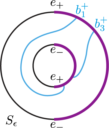
Figure 3.4 Cutting $S_{\epsilon }$
along
$S_{\epsilon }$
along $b_i^+$
yields two disks, each with exactly one interval of
$b_i^+$
yields two disks, each with exactly one interval of $A_\epsilon $
on its boundary. Therefore, we do not need any more cutting arcs.
$A_\epsilon $
on its boundary. Therefore, we do not need any more cutting arcs.
We next define $\tilde a_i$
by pushing the endpoints of
$\tilde a_i$
by pushing the endpoints of $b_i^+$
negatively along the boundary so that
$b_i^+$
negatively along the boundary so that $\tilde a_i$
and
$\tilde a_i$
and $b_i^+$
intersect once transversely. Figure 3.5 shows the arcs
$b_i^+$
intersect once transversely. Figure 3.5 shows the arcs $\tilde a_i$
on
$\tilde a_i$
on $S_\epsilon $
and their mirror images on
$S_\epsilon $
and their mirror images on $-S_0$
. Glued together, they form
$-S_0$
. Glued together, they form $\widetilde {\alpha }_i$
. Since this example has no
$\widetilde {\alpha }_i$
. Since this example has no $\alpha _i$
curves, we have
$\alpha _i$
curves, we have ${\boldsymbol {\alpha }}= \{\widetilde \alpha _i\}_{i\in H_+}$
.
${\boldsymbol {\alpha }}= \{\widetilde \alpha _i\}_{i\in H_+}$
.

Figure 3.5 The $\widetilde {\alpha }_i$
curves obtained from the
$\widetilde {\alpha }_i$
curves obtained from the $b_i^+$
arcs.
$b_i^+$
arcs.
Finally, Figure 3.6 illustrates the bordered sutured Heegaard diagram adapted to the sorted foliated open book of Example 2.24. In this example, the set of intersection points $\mathbf {x}$
consists only of
$\mathbf {x}$
consists only of $x_i^+ = \tilde a_i\cap b_i^+\in S_{\epsilon }$
for
$x_i^+ = \tilde a_i\cap b_i^+\in S_{\epsilon }$
for $i\in H_+$
.
$i\in H_+$
.

Figure 3.6 The bordered sutured Heegaard diagram adapted to the sorted foliated open book of Example 2.24. The intersection points $x_i^+ = \tilde a_i\cap b_i^+\in S_{\epsilon }$
for
$x_i^+ = \tilde a_i\cap b_i^+\in S_{\epsilon }$
for $i\in H_+$
are marked as black dots. The black portion of the resulting boundary is Z, while the green is
$i\in H_+$
are marked as black dots. The black portion of the resulting boundary is Z, while the green is $\partial \Sigma \setminus Z$
.
$\partial \Sigma \setminus Z$
.
We will use $\mathbf {x}$
to define two contact invariants in bordered sutured Floer homology. In order to do that, we first show that
$\mathbf {x}$
to define two contact invariants in bordered sutured Floer homology. In order to do that, we first show that $\mathcal {H}$
is an admissible diagram for the bordered sutured manifold associated to
$\mathcal {H}$
is an admissible diagram for the bordered sutured manifold associated to $(M,\xi ,\mathcal {F})$
.
$(M,\xi ,\mathcal {F})$
.
Proposition 3.4. Let $(\{S_i\},h, \{\gamma _i^\pm \})$
be a sorted abstract foliated open book supporting a foliated contact three-manifold
$(\{S_i\},h, \{\gamma _i^\pm \})$
be a sorted abstract foliated open book supporting a foliated contact three-manifold $(M,\xi ,\mathcal {F})$
. Suppose
$(M,\xi ,\mathcal {F})$
. Suppose $\mathcal {H} = (\Sigma , {\boldsymbol {\alpha }},{\boldsymbol {\beta }},\mathcal Z)$
is a bordered sutured Heegaard diagram adapted to
$\mathcal {H} = (\Sigma , {\boldsymbol {\alpha }},{\boldsymbol {\beta }},\mathcal Z)$
is a bordered sutured Heegaard diagram adapted to $(\{S_i\},h, \{\gamma _i^\pm \})$
. Then
$(\{S_i\},h, \{\gamma _i^\pm \})$
. Then $\mathcal {H}$
gives an admissible bordered Heegaard diagram for the bordered sutured manifold
$\mathcal {H}$
gives an admissible bordered Heegaard diagram for the bordered sutured manifold $(M,\mathsf {\Gamma },\mathcal Z)$
associated to
$(M,\mathsf {\Gamma },\mathcal Z)$
associated to $(M,\xi ,\mathcal {F})$
.
$(M,\xi ,\mathcal {F})$
.
Proof. Starting from a sorted foliated open book $(\{S_i\},h, \{\gamma _i^\pm \})$
, we may either first construct a foliated contact manifold
$(\{S_i\},h, \{\gamma _i^\pm \})$
, we may either first construct a foliated contact manifold $(M,\xi ,\mathcal {F})$
as in Section 2.3.1 and an associated bordered sutured manifold
$(M,\xi ,\mathcal {F})$
as in Section 2.3.1 and an associated bordered sutured manifold $(M,\mathsf {\Gamma },\mathcal Z)$
as in Section 3.1, or we may start by constructing a bordered sutured Heegaard diagram
$(M,\mathsf {\Gamma },\mathcal Z)$
as in Section 3.1, or we may start by constructing a bordered sutured Heegaard diagram $\mathcal {H} = (\Sigma , {\boldsymbol {\alpha }},{\boldsymbol {\beta }},\mathcal Z)$
as above. To temporarily distinguish between the two constructions of the set of matched arcs, we will in fact temporarily replace this notation with
$\mathcal {H} = (\Sigma , {\boldsymbol {\alpha }},{\boldsymbol {\beta }},\mathcal Z)$
as above. To temporarily distinguish between the two constructions of the set of matched arcs, we will in fact temporarily replace this notation with $\mathcal {H} = (\Sigma , {\boldsymbol {\alpha }},{\boldsymbol {\beta }},\mathcal Z')$
, with
$\mathcal {H} = (\Sigma , {\boldsymbol {\alpha }},{\boldsymbol {\beta }},\mathcal Z')$
, with $Z'$
the set of arcs in
$Z'$
the set of arcs in $\mathcal Z'$
. We may then use the construction of Section 2.2.2 to produce a bordered sutured manifold. We wish to verify that the bordered sutured manifold arising this way is
$\mathcal Z'$
. We may then use the construction of Section 2.2.2 to produce a bordered sutured manifold. We wish to verify that the bordered sutured manifold arising this way is $(M, \mathsf {\Gamma }, \mathcal Z)$
.
$(M, \mathsf {\Gamma }, \mathcal Z)$
.
Recall that the foliated contact manifold $(M, \xi , \mathcal {F})$
is built via saddle cobordisms specified by the sorting arcs. We intend for the
$(M, \xi , \mathcal {F})$
is built via saddle cobordisms specified by the sorting arcs. We intend for the $\alpha $
curves to specify the handlebody from
$\alpha $
curves to specify the handlebody from $S_0$
to
$S_0$
to $S_{\epsilon }$
and for the
$S_{\epsilon }$
and for the $\beta $
curves to specify the handlebody from
$\beta $
curves to specify the handlebody from $S_{\epsilon }$
to
$S_{\epsilon }$
to $S_0$
. We will start by modifying the graph
$S_0$
. We will start by modifying the graph $G(\mathcal Z')\subset \Sigma $
and the bordered sutured structure on
$G(\mathcal Z')\subset \Sigma $
and the bordered sutured structure on $\partial M$
via isotopy, allowing us to identify the Heegaard surface
$\partial M$
via isotopy, allowing us to identify the Heegaard surface $\Sigma $
with the surface
$\Sigma $
with the surface $S_\epsilon \cup _B-S_0$
in M in such a way that
$S_\epsilon \cup _B-S_0$
in M in such a way that $\partial \Sigma \setminus Z'$
is identified with
$\partial \Sigma \setminus Z'$
is identified with $\mathsf {\Gamma }$
. (This is equivalent to recovering
$\mathsf {\Gamma }$
. (This is equivalent to recovering $\mathsf {\Gamma }$
as
$\mathsf {\Gamma }$
as $(\partial \Sigma \setminus Z') \times \{\frac {1}{2}\}$
in a thickened copy of the surface
$(\partial \Sigma \setminus Z') \times \{\frac {1}{2}\}$
in a thickened copy of the surface $\Sigma \times [0,1]$
.) Recall that we chose
$\Sigma \times [0,1]$
.) Recall that we chose $Z'$
to be the union of
$Z'$
to be the union of $A_0$
with the arcs
$A_0$
with the arcs $\bigcup _{I\subset A_{\epsilon }}(I_+\cup I_-)$
; the purpose of this choice is to enable a simple discussion of gluing in Section 5. However, we may isotope
$\bigcup _{I\subset A_{\epsilon }}(I_+\cup I_-)$
; the purpose of this choice is to enable a simple discussion of gluing in Section 5. However, we may isotope $Z'$
inward along the arcs
$Z'$
inward along the arcs $I_{\pm }$
to
$I_{\pm }$
to $A_0$
. On
$A_0$
. On $\partial M$
, we may isotope Z (resp.
$\partial M$
, we may isotope Z (resp. $\mathsf {\Gamma }$
) through the disks bounded between Z and
$\mathsf {\Gamma }$
) through the disks bounded between Z and $A_0$
(resp.
$A_0$
(resp. $A_0$
and
$A_0$
and $A_\epsilon $
) and identify it with
$A_\epsilon $
) and identify it with $A_0$
(resp.
$A_0$
(resp. $A_\epsilon $
). This isotopy can be chosen so that it carries the matched points on Z to the matched points on
$A_\epsilon $
). This isotopy can be chosen so that it carries the matched points on Z to the matched points on $Z'$
(as identified with
$Z'$
(as identified with $A_0$
). Note that under this isotopy the edges
$A_0$
). Note that under this isotopy the edges $e_i$
of the graph
$e_i$
of the graph $G(\mathcal Z)$
will twist near their endpoints around the elliptic points.
$G(\mathcal Z)$
will twist near their endpoints around the elliptic points.
Next, $\{\widetilde {a}_i\}_{i\in H_+}\cup \{a_1,\cdots ,a_{2g_0+n_0+|A_0|-k-2}\}$
is a cut system for
$\{\widetilde {a}_i\}_{i\in H_+}\cup \{a_1,\cdots ,a_{2g_0+n_0+|A_0|-k-2}\}$
is a cut system for $S_{\epsilon }$
. At each time
$S_{\epsilon }$
. At each time $0\leq t\leq \epsilon $
, we may consider the image of each of these arcs on
$0\leq t\leq \epsilon $
, we may consider the image of each of these arcs on $\pi ^{-1}(t)$
coming from applying the flow of
$\pi ^{-1}(t)$
coming from applying the flow of $\pi $
; for each arc, the union of these images is a disk with boundary the corresponding
$\pi $
; for each arc, the union of these images is a disk with boundary the corresponding $\alpha $
-circle. (We say that these arcs trace out disks in time
$\alpha $
-circle. (We say that these arcs trace out disks in time $[0,\epsilon ]$
whose boundaries are the
$[0,\epsilon ]$
whose boundaries are the $\alpha $
-circles.) So,
$\alpha $
-circles.) So, ${\boldsymbol {\alpha }}$
specifies the handlebody from
${\boldsymbol {\alpha }}$
specifies the handlebody from $S_0$
to
$S_0$
to $S_{\epsilon }$
. Similarly, the cutting arcs
$S_{\epsilon }$
. Similarly, the cutting arcs $\{b_1,\cdots ,b_{2g_0+n_0+|A_0|-k-2}\}$
for
$\{b_1,\cdots ,b_{2g_0+n_0+|A_0|-k-2}\}$
for $P_\epsilon $
will trace out disks in time
$P_\epsilon $
will trace out disks in time $[\epsilon ,2\pi ]$
, whose boundaries under the identification of
$[\epsilon ,2\pi ]$
, whose boundaries under the identification of $S_{2\pi }$
with
$S_{2\pi }$
with $S_0$
using monodromy h are the
$S_0$
using monodromy h are the $\beta $
-circles on
$\beta $
-circles on $\Sigma $
.
$\Sigma $
.
Finally, for each $i\in H_-$
, flowing backward from time
$i\in H_-$
, flowing backward from time $t=i\pi /k$
to
$t=i\pi /k$
to $t=\epsilon $
, the sorting arc
$t=\epsilon $
, the sorting arc $\gamma _i^-$
traces out a disk corresponding to the cocore of the handle addition. The boundary of this disk is the arc
$\gamma _i^-$
traces out a disk corresponding to the cocore of the handle addition. The boundary of this disk is the arc $\beta ^-_i$
together with the twisted and truncated copy of the separatrix
$\beta ^-_i$
together with the twisted and truncated copy of the separatrix $\delta _i$
, that is, with the twisted arc
$\delta _i$
, that is, with the twisted arc $e_i$
. These are the disks attached along the arcs
$e_i$
. These are the disks attached along the arcs $\beta ^-_i$
. Likewise, for
$\beta ^-_i$
. Likewise, for $i\in H_+$
, flowing forward from
$i\in H_+$
, flowing forward from $t=i\pi /k$
to
$t=i\pi /k$
to $t=2\pi $
, the sorting arc
$t=2\pi $
, the sorting arc $\gamma _i^+$
traces out a disk corresponding to the cutting arc for the handle subtraction, whose boundary under the identification of
$\gamma _i^+$
traces out a disk corresponding to the cutting arc for the handle subtraction, whose boundary under the identification of $S_{2\pi }$
with
$S_{2\pi }$
with $S_0$
via the monodromy h is the arc
$S_0$
via the monodromy h is the arc $\beta _i^+$
together with the twisted and truncated copy of the separatrix
$\beta _i^+$
together with the twisted and truncated copy of the separatrix $\delta _i$
. These are the disks attached along the arcs
$\delta _i$
. These are the disks attached along the arcs $\beta ^+_i$
.
$\beta ^+_i$
.
As for admissibility, we notice that just as in the closed or sutured cases, admissibility is automatic: Every periodic domain with an $\alpha $
-circle on its boundary crosses the only intersection of that circle with
$\alpha $
-circle on its boundary crosses the only intersection of that circle with ${\boldsymbol {\beta }}$
curves or circles on
${\boldsymbol {\beta }}$
curves or circles on $S_{\epsilon }$
, at which point the sign of the connected component of
$S_{\epsilon }$
, at which point the sign of the connected component of $\Sigma \setminus ({\boldsymbol {\alpha }}\cup {\boldsymbol {\beta }})$
must change.
$\Sigma \setminus ({\boldsymbol {\alpha }}\cup {\boldsymbol {\beta }})$
must change.
If $\mathcal {H}$
is a bordered sutured Heegaard diagram adapted to a sorted abstract foliated open book
$\mathcal {H}$
is a bordered sutured Heegaard diagram adapted to a sorted abstract foliated open book $(\{S_i\},h, \{\gamma _i^\pm \})$
and
$(\{S_i\},h, \{\gamma _i^\pm \})$
and $(\{S_i\},h, \{\gamma _i^\pm \})$
is compatible with the foliated contact three-manifold
$(\{S_i\},h, \{\gamma _i^\pm \})$
is compatible with the foliated contact three-manifold $(M,\xi ,\mathcal {F})$
, we say that
$(M,\xi ,\mathcal {F})$
, we say that $\mathcal {H}$
is adapted to
$\mathcal {H}$
is adapted to $(M,\xi ,\mathcal {F})$
.
$(M,\xi ,\mathcal {F})$
.
By Proposition 3.4 and [Reference ZarevZar10, Section 3.4], the diagram ${\overline {\mathcal H}=(\Sigma , {\boldsymbol {\beta }},{\boldsymbol {\alpha }},\overline {\mathcal Z})}$
obtained by exchanging the roles of the two sets of curves and formally replacing the arc diagram
${\overline {\mathcal H}=(\Sigma , {\boldsymbol {\beta }},{\boldsymbol {\alpha }},\overline {\mathcal Z})}$
obtained by exchanging the roles of the two sets of curves and formally replacing the arc diagram $\mathcal Z$
of
$\mathcal Z$
of $\beta $
-type (which is to say, parametrized by arcs which are part of the second set of curves) with the identical arc diagram
$\beta $
-type (which is to say, parametrized by arcs which are part of the second set of curves) with the identical arc diagram $\overline {\mathcal Z}$
of
$\overline {\mathcal Z}$
of $\alpha $
-type (parametrized by arcs which are part of the first set of curves) is a bordered sutured diagram for
$\alpha $
-type (parametrized by arcs which are part of the first set of curves) is a bordered sutured diagram for $(-M,\mathsf {\Gamma },\overline {\mathcal Z})$
. Write
$(-M,\mathsf {\Gamma },\overline {\mathcal Z})$
. Write $\overline {\mathcal Z}=(Z, a, m)$
. We have the following proposition.
$\overline {\mathcal Z}=(Z, a, m)$
. We have the following proposition.
Proposition 3.5. The above $\mathbf {x}$
gives a well-defined generator
$\mathbf {x}$
gives a well-defined generator
 $$\begin{align*}\mathbf{x}_D := \mathbf{x}\in \widehat{\mathit{BSD}}(\overline{\mathcal{H}}) \end{align*}$$
with $I_D(\mathbf {x}) = I(H_-)$
and
$I_D(\mathbf {x}) = I(H_-)$
and $\delta ^1(\mathbf {x}_D) = 0$
, and a well-defined generator
$\delta ^1(\mathbf {x}_D) = 0$
, and a well-defined generator
 $$\begin{align*}\mathbf{x}_A := \mathbf{x}\in \widehat{\mathit{BSA}}(\overline{\mathcal{H}}) \end{align*}$$
with $I_A(\mathbf {x}_A) = I(H_+)$
and
$I_A(\mathbf {x}_A) = I(H_+)$
and $m_{i+1}(\mathbf {x}_A, a(\boldsymbol \rho _1), \ldots , a(\boldsymbol \rho _i))=0$
for all
$m_{i+1}(\mathbf {x}_A, a(\boldsymbol \rho _1), \ldots , a(\boldsymbol \rho _i))=0$
for all $i\geq 0$
and all sets of Reeb chords
$i\geq 0$
and all sets of Reeb chords $\boldsymbol \rho _j$
in
$\boldsymbol \rho _j$
in $(Z, a)$
.
$(Z, a)$
.
Proof. Since each of the intersections in the definition of $\mathbf {x}$
is unique, the two generators are well defined. The idempotents are as stated since the
$\mathbf {x}$
is unique, the two generators are well defined. The idempotents are as stated since the $\beta $
-arcs occupied by
$\beta $
-arcs occupied by $\mathbf {x}$
are indexed by
$\mathbf {x}$
are indexed by $H_+$
, whereas the unoccupied
$H_+$
, whereas the unoccupied $\beta $
-arcs are indexed by
$\beta $
-arcs are indexed by $H_-$
. Last, consider regions of
$H_-$
. Last, consider regions of $\Sigma \setminus ({\boldsymbol {\alpha }}\cup {\boldsymbol {\beta }})$
that have a point
$\Sigma \setminus ({\boldsymbol {\alpha }}\cup {\boldsymbol {\beta }})$
that have a point $x\in \mathbf {x}$
as a corner vertex. Each such region either has an interval of
$x\in \mathbf {x}$
as a corner vertex. Each such region either has an interval of $\partial \Sigma \setminus Z$
on its boundary or it has some corner near which it agrees with one of the thin strips obtained by perturbing the
$\partial \Sigma \setminus Z$
on its boundary or it has some corner near which it agrees with one of the thin strips obtained by perturbing the $b_i$
and
$b_i$
and $b_j^+$
arcs to
$b_j^+$
arcs to $a_i$
and
$a_i$
and $\tilde a_j$
arcs. The positively oriented boundary of such a thin strip near x has a segment of a
$\tilde a_j$
arcs. The positively oriented boundary of such a thin strip near x has a segment of a $\beta $
curve ending at x, and a segment of an
$\beta $
curve ending at x, and a segment of an $\alpha $
curve starting at x. Such a region cannot be in the projection
$\alpha $
curve starting at x. Such a region cannot be in the projection $\pi _{\Sigma }\circ u$
of an index
$\pi _{\Sigma }\circ u$
of an index $1$
holomorphic map
$1$
holomorphic map
 $$\begin{align*}u:(S, \partial S) \to (\operatorname{\mathrm{Int}}(\Sigma)\times \mathbb D \times \mathbb{R}, ({\boldsymbol{\beta}}\times \{1\}\times \mathbb{R})\cup ({\boldsymbol{\alpha}}\times \{0\}\times \mathbb{R}))\end{align*}$$
satisfying [Reference ZarevZar10, Section 5.2, Conditions (1)-(11)] and asymptotic to $\mathbf {x}\times [0,1]$
at
$\mathbf {x}\times [0,1]$
at $-\infty $
. Thus,
$-\infty $
. Thus, $\delta ^1(\mathbf {x}_D) = 0$
, and
$\delta ^1(\mathbf {x}_D) = 0$
, and $m_{i+1}(\mathbf {x}_A, a_1, \ldots , a_i)=0$
for all
$m_{i+1}(\mathbf {x}_A, a_1, \ldots , a_i)=0$
for all $i\geq 0$
and all
$i\geq 0$
and all $a_j\in \mathcal A(\partial \overline {\mathcal {H}})$
.
$a_j\in \mathcal A(\partial \overline {\mathcal {H}})$
.
4 Invariance
In this section, we complete the proof of Theorem 1. Specifically, we show that given two different sets of choices made in constructing a bordered sutured Heegaard diagram for the bordered sutured three-manifold ${(-M,\mathsf {\Gamma }, \overline {\mathcal Z})}$
associated to a foliated contact three-manifold
${(-M,\mathsf {\Gamma }, \overline {\mathcal Z})}$
associated to a foliated contact three-manifold $(M,\xi , \mathcal {F})$
resulting in Heegaard diagrams
$(M,\xi , \mathcal {F})$
resulting in Heegaard diagrams $\mathcal H$
and
$\mathcal H$
and $\mathcal H'$
with associated type A bordered sutured Floer homologies
$\mathcal H'$
with associated type A bordered sutured Floer homologies $\widehat {\mathit {BSA}}(\mathcal H)$
and
$\widehat {\mathit {BSA}}(\mathcal H)$
and $\widehat {\mathit {BSA}}(\mathcal H')$
, the contact elements
$\widehat {\mathit {BSA}}(\mathcal H')$
, the contact elements $\mathbf {x}_A$
and
$\mathbf {x}_A$
and $\mathbf {x}^{\prime }_A$
are equivalent in the sense of Section 2.2.2 and likewise for
$\mathbf {x}^{\prime }_A$
are equivalent in the sense of Section 2.2.2 and likewise for $\mathbf {x}_D$
and
$\mathbf {x}_D$
and $\mathbf {x}_D'$
. We prove equivalence of these classes under
$\mathbf {x}_D'$
. We prove equivalence of these classes under
-
1. isotopy of the monodromy h of the foliated open book
$(\{S_i\},h, \{\gamma _i^\pm \})$
for
$(M,\xi , \mathcal {F})$
; -
2. the choice of complex structure;
-
3. stabilizations of the foliated open book
$(\{S_i\},h, \{\gamma _i^\pm \})$
on the
$S_0$
page; and -
4. the choice of the cutting arcs made when constructing the bordered Heegaard diagram in Section 3.2.


Note that we do not have to prove invariance under time shift since the definition of a triple $(M,\xi , \mathcal {F})$
has an implicit choice of initial time
$(M,\xi , \mathcal {F})$
has an implicit choice of initial time $t=0$
; see Remark 2.15. Invariance under the choice of complex structure follows from [Reference ZarevZar09, Theorem 7.8] and the observation that since there are no nontrivial topological domains beginning at the generator
$t=0$
; see Remark 2.15. Invariance under the choice of complex structure follows from [Reference ZarevZar09, Theorem 7.8] and the observation that since there are no nontrivial topological domains beginning at the generator $\textbf {x}$
on the bordered sutured Heegaard diagram
$\textbf {x}$
on the bordered sutured Heegaard diagram $\mathcal H$
, the type A and type D chain homotopy equivalences between bordered sutured complexes associated to pairs
$\mathcal H$
, the type A and type D chain homotopy equivalences between bordered sutured complexes associated to pairs $(\mathcal H, J_1)$
and
$(\mathcal H, J_1)$
and $(\mathcal H, J_2)$
count a single pseudoholomorphic strip constant in the
$(\mathcal H, J_2)$
count a single pseudoholomorphic strip constant in the $\Sigma $
coordinate beginning at
$\Sigma $
coordinate beginning at $\mathbf {x}_D$
or
$\mathbf {x}_D$
or $\mathbf {x}_A$
, and thus in each case carry the special generator to itself. It is a consequence of Theorem 2.23 that stabilizations on the
$\mathbf {x}_A$
, and thus in each case carry the special generator to itself. It is a consequence of Theorem 2.23 that stabilizations on the $S_0$
page are sufficient.
$S_0$
page are sufficient.
We thus focus on the remaining three choices made in the construction of the contact invariants. For invariance under the isotopy class of h and choice of the cutting arcs, our proofs heavily parallel those of [Reference Honda, Kazez and MatićHKM09b, Section 3] and [Reference Honda, Kazez and MatićHKM09a, Section 3]; our proof of stabilization invariance has a slightly different structure.
Proposition 4.1. Suppose we choose two representatives for the isotopy class of h, resulting in bordered sutured Heegaard diagrams $\mathcal H$
and
$\mathcal H$
and $\mathcal H'$
. The resulting contact elements
$\mathcal H'$
. The resulting contact elements $\mathbf {x}_A \in \widehat {\mathit {BSA}}(\mathcal H)$
and
$\mathbf {x}_A \in \widehat {\mathit {BSA}}(\mathcal H)$
and $\mathbf {x}^{\prime }_A \in \widehat {\mathit {BSA}}(\mathcal H')$
are equivalent in the sense of Section 2.2.2 and likewise for
$\mathbf {x}^{\prime }_A \in \widehat {\mathit {BSA}}(\mathcal H')$
are equivalent in the sense of Section 2.2.2 and likewise for $\mathbf {x}_D$
and
$\mathbf {x}_D$
and $\mathbf {x}_D'$
.
$\mathbf {x}_D'$
.
Proof. The proof given in [Reference Honda, Kazez and MatićHKM09b, Lemma 3.3] carries over to the bordered sutured case essentially verbatim. As previously, the point is that there are no holomorphic curves beginning at the generators $\mathbf {x}_A$
and
$\mathbf {x}_A$
and $\mathbf {x}_D$
.
$\mathbf {x}_D$
.
We now turn our attention to equivalence under choice of the cutting arcs in the case that we start with a sufficiently stabilized foliated open book. (Subsequently, in Proposition 4.5, we will prove stabilization invariance, thus showing invariance of the choice of cutting arcs for all sorted foliated open books.)
First, we show that two different choices of cutting arcs ${\boldsymbol b}$
and
${\boldsymbol b}$
and $\widetilde {{\boldsymbol b}}$
for
$\widetilde {{\boldsymbol b}}$
for $P_{\epsilon }\subset S_{\epsilon }$
are related by arcslides on
$P_{\epsilon }\subset S_{\epsilon }$
are related by arcslides on $P_{\epsilon }$
.
$P_{\epsilon }$
.
Proposition 4.2. Suppose that $(\{S_i\},h,\{\gamma _i\})$
is a sufficiently stabilized foliated open book. Then any two sets of cutting arcs
$(\{S_i\},h,\{\gamma _i\})$
is a sufficiently stabilized foliated open book. Then any two sets of cutting arcs ${\boldsymbol b} = \{b_1, \ldots , b_{2g_0+n_0+|A_0|-k-2}\}$
and
${\boldsymbol b} = \{b_1, \ldots , b_{2g_0+n_0+|A_0|-k-2}\}$
and $\widetilde {{\boldsymbol b}} = \{\widetilde {b}_1, \ldots , \widetilde {b}_{2g_0+n_0+|A_0|-k-2}\}$
for
$\widetilde {{\boldsymbol b}} = \{\widetilde {b}_1, \ldots , \widetilde {b}_{2g_0+n_0+|A_0|-k-2}\}$
for $P_{\epsilon }$
are related by a sequence of arcslides.
$P_{\epsilon }$
are related by a sequence of arcslides.
Proof. The proof is modeled on [Reference Honda, Kazez and MatićHKM09a, Lemma 3.3] and [Reference Honda, Kazez and MatićHKM09b, Lemma 3.6]. Let $r=2g_0+n_0+|A_0|-k-2$
.
$r=2g_0+n_0+|A_0|-k-2$
.
First, we will show that $\cup _{i=1}^r b_i$
and
$\cup _{i=1}^r b_i$
and $\cup _{i=1}^r \widetilde {b}_i$
can be made disjoint from each other by performing a sequence of arcslides. Then we verify the statement of the proposition for the case of two disjoint sets of cutting arcs. Suppose that
$\cup _{i=1}^r \widetilde {b}_i$
can be made disjoint from each other by performing a sequence of arcslides. Then we verify the statement of the proposition for the case of two disjoint sets of cutting arcs. Suppose that $\left (\cup _{i=1}^r b_i\right )\cap \left (\cup _{i=1}^r \widetilde {b}_i\right )\neq \emptyset $
. We may assume the curves intersect efficiently. We can decrease the number of intersections as follows.
$\left (\cup _{i=1}^r b_i\right )\cap \left (\cup _{i=1}^r \widetilde {b}_i\right )\neq \emptyset $
. We may assume the curves intersect efficiently. We can decrease the number of intersections as follows.
Cut $P_{\epsilon }$
along the arcs in
$P_{\epsilon }$
along the arcs in ${\boldsymbol b}$
to obtain a set of polygons. For each cutting arc
${\boldsymbol b}$
to obtain a set of polygons. For each cutting arc $b_i$
, label the two resulting boundary segments on
$b_i$
, label the two resulting boundary segments on $\partial (P_{\epsilon }\setminus {\boldsymbol b})$
by
$\partial (P_{\epsilon }\setminus {\boldsymbol b})$
by $b_i$
and
$b_i$
and $b_i^{-1}$
and call these two segments partners.
$b_i^{-1}$
and call these two segments partners.
First, we show that every connected component of $P_\epsilon \setminus \boldsymbol {b}$
intersects
$P_\epsilon \setminus \boldsymbol {b}$
intersects $R_\epsilon $
in exactly one interval. To see that each connected component of
$R_\epsilon $
in exactly one interval. To see that each connected component of $P_\epsilon \setminus \boldsymbol {b}$
intersects
$P_\epsilon \setminus \boldsymbol {b}$
intersects $R_\epsilon $
, observe that otherwise the boundary of the component would only contain arcs in B and in
$R_\epsilon $
, observe that otherwise the boundary of the component would only contain arcs in B and in $\boldsymbol {b}$
. But the connected components of
$\boldsymbol {b}$
. But the connected components of $P_\epsilon \setminus \boldsymbol {b}$
are naturally identified with the connected components of
$P_\epsilon \setminus \boldsymbol {b}$
are naturally identified with the connected components of $S_{\epsilon }\setminus ({\boldsymbol b}\cup {\boldsymbol {\beta }}^a)$
and by the definition of cutting arcs, each connected component of
$S_{\epsilon }\setminus ({\boldsymbol b}\cup {\boldsymbol {\beta }}^a)$
and by the definition of cutting arcs, each connected component of $S_{\epsilon }\setminus ({\boldsymbol b}\cup {\boldsymbol {\beta }}^a)$
is a disk with exactly one interval of
$S_{\epsilon }\setminus ({\boldsymbol b}\cup {\boldsymbol {\beta }}^a)$
is a disk with exactly one interval of $A_{\epsilon }$
on its boundary. Moreover,
$A_{\epsilon }$
on its boundary. Moreover, $P_\epsilon \setminus \boldsymbol {b}$
cannot intersect
$P_\epsilon \setminus \boldsymbol {b}$
cannot intersect $R_\epsilon $
in more intervals. Assume it intersects
$R_\epsilon $
in more intervals. Assume it intersects $R_\epsilon $
in at least two intervals. There are two types of such a segment of
$R_\epsilon $
in at least two intervals. There are two types of such a segment of $R_\epsilon $
: Either it corresponds only to an arc in
$R_\epsilon $
: Either it corresponds only to an arc in $A_\epsilon $
or also to an arc of type
$A_\epsilon $
or also to an arc of type $\gamma ^\pm _i$
whose both endpoints connect to arcs in
$\gamma ^\pm _i$
whose both endpoints connect to arcs in $A_\epsilon $
. In this latter case, the isotopy of
$A_\epsilon $
. In this latter case, the isotopy of $\gamma ^\pm _i$
resulting in
$\gamma ^\pm _i$
resulting in ${\boldsymbol {\beta }}^\pm _i$
leaves at least one of these arcs in
${\boldsymbol {\beta }}^\pm _i$
leaves at least one of these arcs in $A_\epsilon $
on the boundary of the connected component of
$A_\epsilon $
on the boundary of the connected component of $S_{\epsilon }\setminus ({\boldsymbol b}\cup {\boldsymbol {\beta }}^a)$
. In the former case, the only arc in
$S_{\epsilon }\setminus ({\boldsymbol b}\cup {\boldsymbol {\beta }}^a)$
. In the former case, the only arc in $A_\epsilon $
is also on the boundary of the corresponding connected component of
$A_\epsilon $
is also on the boundary of the corresponding connected component of $S_{\epsilon }\setminus ({\boldsymbol b}\cup {\boldsymbol {\beta }}^a)$
. In both cases, the segment of
$S_{\epsilon }\setminus ({\boldsymbol b}\cup {\boldsymbol {\beta }}^a)$
. In both cases, the segment of $R_\epsilon $
corresponds to an arc in
$R_\epsilon $
corresponds to an arc in $A_\epsilon $
on
$A_\epsilon $
on $\partial S_{\epsilon }\setminus ({\boldsymbol b}\cup {\boldsymbol {\beta }}^a)$
. Therefore, our assumption contradicts the fact that
$\partial S_{\epsilon }\setminus ({\boldsymbol b}\cup {\boldsymbol {\beta }}^a)$
. Therefore, our assumption contradicts the fact that $S_{\epsilon }\setminus ({\boldsymbol b}\cup {\boldsymbol {\beta }}^a)$
contains exactly one interval of
$S_{\epsilon }\setminus ({\boldsymbol b}\cup {\boldsymbol {\beta }}^a)$
contains exactly one interval of $A_{\epsilon }$
on its boundary.
$A_{\epsilon }$
on its boundary.
Consider a connected component C of $P_{\epsilon }\setminus {\boldsymbol b}$
containing an intersection point of
$P_{\epsilon }\setminus {\boldsymbol b}$
containing an intersection point of $\cup _{i=1}^r b_i$
and
$\cup _{i=1}^r b_i$
and $\cup _{i=1}^r \widetilde {b}_i$
. Then C is a polygon with some number of edges in
$\cup _{i=1}^r \widetilde {b}_i$
. Then C is a polygon with some number of edges in ${\boldsymbol b}$
(of types
${\boldsymbol b}$
(of types $b_j$
and
$b_j$
and $b_j^{-1}$
), some number of edges in B and exactly one edge in
$b_j^{-1}$
), some number of edges in B and exactly one edge in $R_{\epsilon }$
.
$R_{\epsilon }$
.
After possibly reordering the elements of ${\boldsymbol b}$
, we may assume that
${\boldsymbol b}$
, we may assume that $b_1 \cap \widetilde {b}_1\neq \emptyset $
and that we can find a subarc
$b_1 \cap \widetilde {b}_1\neq \emptyset $
and that we can find a subarc $\widetilde {b}_1^0\subset \widetilde {b}_1$
in C such that
$\widetilde {b}_1^0\subset \widetilde {b}_1$
in C such that $\widetilde {b}_1^0$
starts from a segment
$\widetilde {b}_1^0$
starts from a segment $B_1$
of the binding B, ends on
$B_1$
of the binding B, ends on $b_1$
and has interior disjoint from
$b_1$
and has interior disjoint from $\cup _{i=1}^r b_i$
, as in Figure 4.1. We may also assume that
$\cup _{i=1}^r b_i$
, as in Figure 4.1. We may also assume that $b_1$
and
$b_1$
and $B_1$
are not adjacent, as we could otherwise isotope
$B_1$
are not adjacent, as we could otherwise isotope $\widetilde {b}_1^0$
to decrease the number of intersection points between
$\widetilde {b}_1^0$
to decrease the number of intersection points between $\widetilde {b}_1^0$
and
$\widetilde {b}_1^0$
and $b_1$
.
$b_1$
.
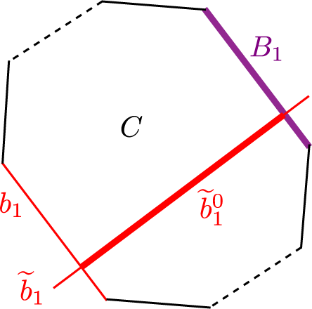
Figure 4.1 The polygon C, with the subarc $\widetilde {b}^0_1$
crossing between the nonadjacent arcs
$\widetilde {b}^0_1$
crossing between the nonadjacent arcs $b_1$
and
$b_1$
and $B_1$
.
$B_1$
.
Now, $\widetilde {b}_1^0$
cuts C into two polygons
$\widetilde {b}_1^0$
cuts C into two polygons $C_1$
and
$C_1$
and $C_2$
, at least one of which does not contain
$C_2$
, at least one of which does not contain $b_1^{-1}$
. Suppose first that
$b_1^{-1}$
. Suppose first that $C_1$
does not contain
$C_1$
does not contain $b_1^{-1}$
and also that
$b_1^{-1}$
and also that $\partial C_1\cap \partial R_{\epsilon }=\emptyset $
. In this case, we may slide
$\partial C_1\cap \partial R_{\epsilon }=\emptyset $
. In this case, we may slide $b_1$
over the remaining arcs in
$b_1$
over the remaining arcs in $\partial C_1$
until we obtain
$\partial C_1$
until we obtain $b^\prime _1$
. Note that
$b^\prime _1$
. Note that $b^{\prime }_1$
has a subarc which lies on
$b^{\prime }_1$
has a subarc which lies on $b_1$
, while the rest of
$b_1$
, while the rest of $b^{\prime }_1$
lies in a small neighborhood of
$b^{\prime }_1$
lies in a small neighborhood of $\widetilde {b}_1$
. This means that no new intersection points are created, while we cancel the one we started with. Therefore,
$\widetilde {b}_1$
. This means that no new intersection points are created, while we cancel the one we started with. Therefore, $b^\prime _1\cup b_2\cup ...\cup b_r$
has fewer intersection points with
$b^\prime _1\cup b_2\cup ...\cup b_r$
has fewer intersection points with $\cup _{i=1}^r \widetilde {b}_i$
. We proceed similarly in the case when
$\cup _{i=1}^r \widetilde {b}_i$
. We proceed similarly in the case when $\partial C_1\cap \partial R_{\epsilon }\neq \emptyset $
but
$\partial C_1\cap \partial R_{\epsilon }\neq \emptyset $
but $b_1^{-1}$
is not contained in
$b_1^{-1}$
is not contained in $\partial C_2$
because then we may slide
$\partial C_2$
because then we may slide $b_1$
over the remaining arcs in
$b_1$
over the remaining arcs in $\partial C_2$
to get
$\partial C_2$
to get $b^\prime _1$
. The case when
$b^\prime _1$
. The case when $\partial C_1$
intersects
$\partial C_1$
intersects $\partial R_{\epsilon }$
in an arc
$\partial R_{\epsilon }$
in an arc $\gamma $
and
$\gamma $
and $C_2$
contains
$C_2$
contains $b_1^{-1}$
on its boundary is handled as follows. Since the foliated open book is sufficiently stabilized, any connected component of
$b_1^{-1}$
on its boundary is handled as follows. Since the foliated open book is sufficiently stabilized, any connected component of $P_{\epsilon }$
intersects
$P_{\epsilon }$
intersects $\partial R_{\epsilon }$
in at least two intervals. Therefore, there is an arc
$\partial R_{\epsilon }$
in at least two intervals. Therefore, there is an arc $c\subset \partial C$
which is of type
$c\subset \partial C$
which is of type $b_i$
or
$b_i$
or $b_i^{-1}$
such that
$b_i^{-1}$
such that $c^{-1}$
is not in
$c^{-1}$
is not in $\partial C$
; otherwise, C would glue up to a connected component of
$\partial C$
; otherwise, C would glue up to a connected component of $P_{\epsilon }$
intersecting
$P_{\epsilon }$
intersecting $\partial R_{\epsilon }$
in only one interval. Sliding c over all other arcs in
$\partial R_{\epsilon }$
in only one interval. Sliding c over all other arcs in $\partial C$
except
$\partial C$
except $\gamma $
gives us
$\gamma $
gives us $c'$
parallel to
$c'$
parallel to $\gamma $
. After this, we may slide
$\gamma $
. After this, we may slide $b_1$
over the arcs in
$b_1$
over the arcs in $\partial C_1$
since now we only need to slide it over
$\partial C_1$
since now we only need to slide it over $c'$
instead of
$c'$
instead of $\gamma $
. Finally, we get
$\gamma $
. Finally, we get $b^\prime _1$
which has a subarc lying on
$b^\prime _1$
which has a subarc lying on $b_1$
, while the rest lie in a small neighborhood of
$b_1$
, while the rest lie in a small neighborhood of $\widetilde {b}_1$
as before. This means that no new intersection points are created, while we cancel the one we started with. Therefore,
$\widetilde {b}_1$
as before. This means that no new intersection points are created, while we cancel the one we started with. Therefore, $\{b^\prime _1,b_2,...,b_r\}$
has fewer intersection points with
$\{b^\prime _1,b_2,...,b_r\}$
has fewer intersection points with $\cup _{i=1}^r \widetilde {b}_i$
than
$\cup _{i=1}^r \widetilde {b}_i$
than $\cup _{i=1}^r b_i$
did. Iterating this procedure a finite number of times, we obtain a new set of cutting arcs which are disjoint from the arcs
$\cup _{i=1}^r b_i$
did. Iterating this procedure a finite number of times, we obtain a new set of cutting arcs which are disjoint from the arcs $\widetilde {\boldsymbol b}$
.
$\widetilde {\boldsymbol b}$
.
Next, we show that for $\cup _{i=1}^r b_i$
and
$\cup _{i=1}^r b_i$
and $\cup _{i=1}^r \widetilde {b}_i$
disjoint,
$\cup _{i=1}^r \widetilde {b}_i$
disjoint, ${\boldsymbol b}$
can be turned into
${\boldsymbol b}$
can be turned into $\widetilde {{\boldsymbol b}}$
via a finite sequence of arcslides. Let C denote a connected component of
$\widetilde {{\boldsymbol b}}$
via a finite sequence of arcslides. Let C denote a connected component of $P_{\epsilon }\setminus {\boldsymbol b}$
as before. If each arc
$P_{\epsilon }\setminus {\boldsymbol b}$
as before. If each arc $\widetilde {b}_i$
in C is parallel to some
$\widetilde {b}_i$
in C is parallel to some $b_j$
or
$b_j$
or $b_j^{-1}$
, we are done with C. Suppose that there is an arc, say
$b_j^{-1}$
, we are done with C. Suppose that there is an arc, say $\widetilde {b}_1$
, which is not parallel to any
$\widetilde {b}_1$
, which is not parallel to any $b_j$
or
$b_j$
or $b_j^{-1}$
. Then
$b_j^{-1}$
. Then $\widetilde {b}_1$
cuts C into two pieces
$\widetilde {b}_1$
cuts C into two pieces $C_1$
and
$C_1$
and $C_2$
, with the property that each
$C_2$
, with the property that each $\partial C_i$
contains more than one arc of type
$\partial C_i$
contains more than one arc of type $b_j$
or
$b_j$
or $b_j^{-1}$
. Choose the labeling such that
$b_j^{-1}$
. Choose the labeling such that $C \cap R_{\epsilon }$
is in
$C \cap R_{\epsilon }$
is in $C_1$
. Moreover, we can find a pair of arcs
$C_1$
. Moreover, we can find a pair of arcs $b_j$
and
$b_j$
and $b_j^{-1}$
such that
$b_j^{-1}$
such that $b_j \subset \partial C_2$
and
$b_j \subset \partial C_2$
and $b_j^{-1}\not \subset \partial C_2$
(or vice versa); otherwise, every segment of
$b_j^{-1}\not \subset \partial C_2$
(or vice versa); otherwise, every segment of $\partial C_2$
has its partner in
$\partial C_2$
has its partner in $\partial C_2$
, implying that some part of
$\partial C_2$
, implying that some part of $C_2$
glues up to a connected component of
$C_2$
glues up to a connected component of $P_{\epsilon }\setminus \boldsymbol {b}$
which does not intersect
$P_{\epsilon }\setminus \boldsymbol {b}$
which does not intersect $R_{\epsilon }$
. If each such
$R_{\epsilon }$
. If each such $b_j$
were parallel to an arc
$b_j$
were parallel to an arc $\widetilde {b}_j$
, then
$\widetilde {b}_j$
, then $\cup _{i=1}^r \widetilde {b}_i$
would again cut off a subsurface which does not intersect
$\cup _{i=1}^r \widetilde {b}_i$
would again cut off a subsurface which does not intersect $R_{\epsilon }$
. Therefore, we may assume that there exists a
$R_{\epsilon }$
. Therefore, we may assume that there exists a $b_j$
which is not parallel to any
$b_j$
which is not parallel to any $\widetilde {b}_l$
. Now, we can slide
$\widetilde {b}_l$
. Now, we can slide $b_j$
over all the arcs
$b_j$
over all the arcs $b_l$
and
$b_l$
and $b_l^{-1}$
in
$b_l^{-1}$
in $C_1$
until it becomes parallel to
$C_1$
until it becomes parallel to $\widetilde {b}_1$
. This way we associated an arc which was not parallel to any
$\widetilde {b}_1$
. This way we associated an arc which was not parallel to any $\widetilde {b}_l$
before to
$\widetilde {b}_l$
before to $\widetilde {b}_1$
not parallel to any
$\widetilde {b}_1$
not parallel to any $b_j$
or
$b_j$
or $b_j^{-1}$
before. Repeating this, we can find a parallel pair for each
$b_j^{-1}$
before. Repeating this, we can find a parallel pair for each $\widetilde {b}_i$
in C.
$\widetilde {b}_i$
in C.
Proposition 4.3. Let $\boldsymbol {b} = \{b_1,b_2, \dots , b_r\} \rightarrow \{b_1 + b_2,b_2 \dots , b_r \} = \boldsymbol {b'}$
be an arcslide among the cutting arcs on
$\boldsymbol {b} = \{b_1,b_2, \dots , b_r\} \rightarrow \{b_1 + b_2,b_2 \dots , b_r \} = \boldsymbol {b'}$
be an arcslide among the cutting arcs on $P_{\epsilon }$
. If
$P_{\epsilon }$
. If $\mathcal H$
and
$\mathcal H$
and $\mathcal H'$
are the resulting bordered sutured Heegaard diagams, then the resulting contact elements
$\mathcal H'$
are the resulting bordered sutured Heegaard diagams, then the resulting contact elements $\mathbf {x}_A \in \widehat {\mathit {BSA}}(\mathcal H)$
and
$\mathbf {x}_A \in \widehat {\mathit {BSA}}(\mathcal H)$
and $\mathbf {x}_A' \in \widehat {\mathit {BSA}}(\mathcal H')$
are equivalent in the sense of Section 2.2.2, and likewise for
$\mathbf {x}_A' \in \widehat {\mathit {BSA}}(\mathcal H')$
are equivalent in the sense of Section 2.2.2, and likewise for $\mathbf {x}_D$
and
$\mathbf {x}_D$
and $\mathbf {x}_D'$
.
$\mathbf {x}_D'$
.
Proof. An arcslide induces a pair of handleslides, one among the $\alpha $
-circles followed by one among their pushoffs, that is, the
$\alpha $
-circles followed by one among their pushoffs, that is, the $\beta $
-circles. The induced maps on
$\beta $
-circles. The induced maps on $\widehat {\mathit {BSD}}$
and on
$\widehat {\mathit {BSD}}$
and on $\widehat {\mathit {BSA}}$
count holomorphic triangles that do not interact with the boundary of the Heegaard diagram. Thus, the proof is a straightforward adaptation of [Reference Honda, Kazez and MatićHKM09b, Lemma 3.5].
$\widehat {\mathit {BSA}}$
count holomorphic triangles that do not interact with the boundary of the Heegaard diagram. Thus, the proof is a straightforward adaptation of [Reference Honda, Kazez and MatićHKM09b, Lemma 3.5].
We conclude the following.
Proposition 4.4. Let ${\boldsymbol b} = \{b_1, \dots , b_r\}$
and
${\boldsymbol b} = \{b_1, \dots , b_r\}$
and $\widetilde {\boldsymbol b} = \{\widetilde {b}_1, \dots , \widetilde {b}_r\}$
be two possible choices of cutting arcs made in the construction of the bordered Heegaard diagram associated to the sufficiently stabilized open book
$\widetilde {\boldsymbol b} = \{\widetilde {b}_1, \dots , \widetilde {b}_r\}$
be two possible choices of cutting arcs made in the construction of the bordered Heegaard diagram associated to the sufficiently stabilized open book $(\{S_i\},h,\{\gamma _i\})$
, and let
$(\{S_i\},h,\{\gamma _i\})$
, and let $\mathcal H$
and
$\mathcal H$
and $\widetilde {\mathcal H}$
be the resulting bordered sutured Heegaard diagrams. Then the resulting contact elements
$\widetilde {\mathcal H}$
be the resulting bordered sutured Heegaard diagrams. Then the resulting contact elements $\mathbf {x}_A \in \widehat {\mathit {BSA}}(\mathcal H)$
and
$\mathbf {x}_A \in \widehat {\mathit {BSA}}(\mathcal H)$
and $\mathbf {x}_A' \in \widehat {\mathit {BSA}}(\mathcal H')$
are equivalent in the sense of Section 2.2.2 and likewise for
$\mathbf {x}_A' \in \widehat {\mathit {BSA}}(\mathcal H')$
are equivalent in the sense of Section 2.2.2 and likewise for $\mathbf {x}_D$
and
$\mathbf {x}_D$
and $\mathbf {x}_D'$
.
$\mathbf {x}_D'$
.
Proposition 4.5. Let $(\{S_i'\},h',\{{\gamma _i'}^\pm \})$
be the open book resulting from stabilization of the open book
$(\{S_i'\},h',\{{\gamma _i'}^\pm \})$
be the open book resulting from stabilization of the open book $(\{S_i\},h,\{\gamma _i^\pm \})$
on the
$(\{S_i\},h,\{\gamma _i^\pm \})$
on the $S_0$
page, and let
$S_0$
page, and let $\mathcal H$
and
$\mathcal H$
and $\mathcal H'$
be the resulting bordered sutured Heegaard diagrams. The resulting contact elements
$\mathcal H'$
be the resulting bordered sutured Heegaard diagrams. The resulting contact elements $\mathbf {x}_A \in \widehat {\mathit {BSA}}(\mathcal H)$
and
$\mathbf {x}_A \in \widehat {\mathit {BSA}}(\mathcal H)$
and $\mathbf {x}_A' \in \widehat {\mathit {BSA}}(\mathcal H')$
are equivalent in the sense of Section 2.2.2 and likewise for type D.
$\mathbf {x}_A' \in \widehat {\mathit {BSA}}(\mathcal H')$
are equivalent in the sense of Section 2.2.2 and likewise for type D.
Proof. Let $\mathcal {H} = (\Sigma , {{\boldsymbol {\alpha }}}, {{\boldsymbol {\beta }}},\mathcal Z)$
be a bordered sutured Heegaard diagram adapted to
$\mathcal {H} = (\Sigma , {{\boldsymbol {\alpha }}}, {{\boldsymbol {\beta }}},\mathcal Z)$
be a bordered sutured Heegaard diagram adapted to $(\{S_i\},h, \{\gamma _i^\pm \})$
. We take
$(\{S_i\},h, \{\gamma _i^\pm \})$
. We take $(\{S_i'\},h', \{{\gamma _i'}^\pm \})$
to be the result of stabilizing
$(\{S_i'\},h', \{{\gamma _i'}^\pm \})$
to be the result of stabilizing $(\{S_i\},h, \{\gamma _i^\pm \})$
along a curve
$(\{S_i\},h, \{\gamma _i^\pm \})$
along a curve $\gamma \subset S_0$
. Recall that if we denote by
$\gamma \subset S_0$
. Recall that if we denote by $\overline {h}$
the extension of h to the added one-handle by the identity, then
$\overline {h}$
the extension of h to the added one-handle by the identity, then $h'=\tau \circ \overline {h}$
, where
$h'=\tau \circ \overline {h}$
, where $\tau $
is a positive Dehn twist along the circle c formed by
$\tau $
is a positive Dehn twist along the circle c formed by $\gamma $
and the core of the attached one-handle. This means that we can obtain from
$\gamma $
and the core of the attached one-handle. This means that we can obtain from $\mathcal {H}$
a diagram
$\mathcal {H}$
a diagram $\mathcal {H}' = (\Sigma ', {{\boldsymbol {\alpha }}'}, {{\boldsymbol {\beta }}'},\mathcal Z)$
adapted to
$\mathcal {H}' = (\Sigma ', {{\boldsymbol {\alpha }}'}, {{\boldsymbol {\beta }}'},\mathcal Z)$
adapted to $(\{S_i'\},h', \{{\gamma _i'}^\pm \})$
as follows. Add a one-handle to the two pages
$(\{S_i'\},h', \{{\gamma _i'}^\pm \})$
as follows. Add a one-handle to the two pages $S_{\epsilon }$
and
$S_{\epsilon }$
and $-S_0$
that form the Heegaard surface in order to obtain
$-S_0$
that form the Heegaard surface in order to obtain $\Sigma ' = S_{\epsilon }'\cup -S_0'$
. Let
$\Sigma ' = S_{\epsilon }'\cup -S_0'$
. Let $b'$
be the cocore of the one-handle on
$b'$
be the cocore of the one-handle on $S_{\epsilon }'$
, and let
$S_{\epsilon }'$
, and let $a'$
be a perturbation of the new cutting arc
$a'$
be a perturbation of the new cutting arc $b'$
to the left. Let
$b'$
to the left. Let
 $$\begin{align*}\beta'=b'\cup -h'\circ \iota(b')\subset S_{\epsilon}'\cup_{B}-S_{0}',\end{align*}$$
and let
 $$\begin{align*}\alpha' = a'\cup -a' \subset S_{\epsilon}'\cup_{B}-S_{0}'.\end{align*}$$
Last, modify all $\beta $
curves that intersect
$\beta $
curves that intersect $\gamma $
by applying to them a positive Dehn twist along c; see Figure 4.2(b). Clearly
$\gamma $
by applying to them a positive Dehn twist along c; see Figure 4.2(b). Clearly $\mathcal {H}'$
is adapted to the stabilized open book
$\mathcal {H}'$
is adapted to the stabilized open book $(\{S_i'\},h', \{{\gamma _i'}^\pm \})$
.
$(\{S_i'\},h', \{{\gamma _i'}^\pm \})$
.
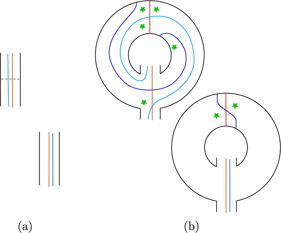
Figure 4.2 (a) The two neighborhoods on $S_{\epsilon }$
and
$S_{\epsilon }$
and $S_0$
of the stabilization arc, viewed on the Heegaard diagram
$S_0$
of the stabilization arc, viewed on the Heegaard diagram $\mathcal H$
. The stabilization arc is drawn as a grey dashed arc on
$\mathcal H$
. The stabilization arc is drawn as a grey dashed arc on $S_0$
. The red and blue vertical lines on each neighborhood represent a (possibly) more general sequence of
$S_0$
. The red and blue vertical lines on each neighborhood represent a (possibly) more general sequence of $\alpha $
and
$\alpha $
and $\beta $
curves. (b) The Heegaard diagram
$\beta $
curves. (b) The Heegaard diagram $\mathcal H'$
corresponding to the stabilized open book, where the same choice of cutting arcs is used away from the stabilization region and the cocore of the stabilizing one-handle is used as the final cutting arc; the diagram
$\mathcal H'$
corresponding to the stabilized open book, where the same choice of cutting arcs is used away from the stabilization region and the cocore of the stabilizing one-handle is used as the final cutting arc; the diagram $\mathcal H'$
has one new
$\mathcal H'$
has one new $\alpha $
circle denoted
$\alpha $
circle denoted $\alpha '$
and one new
$\alpha '$
and one new $\beta $
circle, denoted
$\beta $
circle, denoted $\beta '$
. In this and all subsequent figure in this section, black lines are identified via translation in the plane, being part of the binding. Green stars mark regions that intersect
$\beta '$
. In this and all subsequent figure in this section, black lines are identified via translation in the plane, being part of the binding. Green stars mark regions that intersect $\partial \Sigma \setminus Z$
; to see why the marked regions indeed intersect the
$\partial \Sigma \setminus Z$
; to see why the marked regions indeed intersect the $\partial \Sigma \setminus Z$
part of
$\partial \Sigma \setminus Z$
part of $\partial \Sigma $
nontrivially, simply note that the stabilization arc has endpoints on
$\partial \Sigma $
nontrivially, simply note that the stabilization arc has endpoints on $\partial \Sigma \setminus Z$
.
$\partial \Sigma \setminus Z$
.
Figures 4.2–4.4 demonstrate a sequence of Heegaard moves that transforms $\mathcal {H}'$
into a diagram
$\mathcal {H}'$
into a diagram $\mathcal {H}''$
adapted to a foliated open book
$\mathcal {H}''$
adapted to a foliated open book $(\{S_i\},h'', \{\gamma _i^\pm \})$
whose monodromy
$(\{S_i\},h'', \{\gamma _i^\pm \})$
whose monodromy $h''$
is isotopic to h.
$h''$
is isotopic to h.
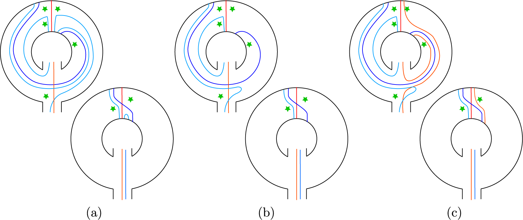
Figure 4.3 (a) The diagram after sliding all $\beta $
curves that intersect
$\beta $
curves that intersect $\alpha '$
over
$\alpha '$
over $\beta '$
to eliminate the intersection points. (b) An isotopy of the previous figure. (c) The result of sliding all
$\beta '$
to eliminate the intersection points. (b) An isotopy of the previous figure. (c) The result of sliding all $\alpha $
circles that intersect
$\alpha $
circles that intersect $\beta '$
over
$\beta '$
over $\alpha '$
, so that the new neighborhood of
$\alpha '$
, so that the new neighborhood of $\alpha '\cup \beta '$
is a punctured torus with a single intersection point of
$\alpha '\cup \beta '$
is a punctured torus with a single intersection point of ${\boldsymbol {\alpha }}'\cap {\boldsymbol {\beta }}'$
.
${\boldsymbol {\alpha }}'\cap {\boldsymbol {\beta }}'$
.

Figure 4.4 (a) The result of excising the punctured torus, along with an isotopy of the curve that represents the binding ‘trading’ two bigons from $S_{\epsilon }$
to
$S_{\epsilon }$
to $S_0$
; the grey lines are the boundary of the punctured torus; the new binding is marked in purple. (b) An isotopy of the previous figure, again with the grey lines as the boundary of a puncture. (c) An isotopy of the previous figure, divided by page according to the new binding.
$S_0$
; the grey lines are the boundary of the punctured torus; the new binding is marked in purple. (b) An isotopy of the previous figure, again with the grey lines as the boundary of a puncture. (c) An isotopy of the previous figure, divided by page according to the new binding.
In particular, in Figure 4.2(a) we see the original neighborhood of $\mathcal {H}'$
where we intend to stabilize, with the stabilization arc drawn in (dashed) grey, and in Figure 4.2(b) we see the result of the stabilization, with new curves
$\mathcal {H}'$
where we intend to stabilize, with the stabilization arc drawn in (dashed) grey, and in Figure 4.2(b) we see the result of the stabilization, with new curves $\alpha '$
and
$\alpha '$
and $\beta '$
. Observe that each of
$\beta '$
. Observe that each of $\alpha '$
and
$\alpha '$
and $\beta '$
may intersect some number of
$\beta '$
may intersect some number of $\alpha $
and
$\alpha $
and $\beta $
curves on
$\beta $
curves on $S_0$
. We handleslide every
$S_0$
. We handleslide every $\beta $
curve other than
$\beta $
curve other than $\beta '$
that intersects
$\beta '$
that intersects $\alpha '$
over
$\alpha '$
over $\beta '$
to obtain Figure 4.3(a), in which we have eliminated all intersection points between
$\beta '$
to obtain Figure 4.3(a), in which we have eliminated all intersection points between $\alpha '$
and any
$\alpha '$
and any $\beta $
curve other than
$\beta $
curve other than $\beta '$
. After a small isotopy of the diagram to Figure 4.3(b), we then handleslide all
$\beta '$
. After a small isotopy of the diagram to Figure 4.3(b), we then handleslide all $\alpha $
circles other than
$\alpha $
circles other than $\alpha '$
which intersect
$\alpha '$
which intersect $\beta '$
over the curve
$\beta '$
over the curve $\alpha '$
. The result of these handleslides, shown in Figure 4.3(c), is a diagram in which
$\alpha '$
. The result of these handleslides, shown in Figure 4.3(c), is a diagram in which $\alpha '$
and
$\alpha '$
and $\beta '$
intersect once and there is a punctured torus neighborhood of
$\beta '$
intersect once and there is a punctured torus neighborhood of $\alpha '\cup \beta '$
which intersects no other
$\alpha '\cup \beta '$
which intersects no other $\alpha $
or
$\alpha $
or $\beta $
curves. We excise this punctured torus, obtaining Figure 4.4(a), after which we may isotope the surface to obtain Figure 4.4(b); trading two bigons between
$\beta $
curves. We excise this punctured torus, obtaining Figure 4.4(a), after which we may isotope the surface to obtain Figure 4.4(b); trading two bigons between $S_0$
and
$S_0$
and $S_{\epsilon }$
produces the diagram
$S_{\epsilon }$
produces the diagram $\mathcal {H}''$
shown in Figure 4.4(c), whose monodromy
$\mathcal {H}''$
shown in Figure 4.4(c), whose monodromy $h''$
is isotopic to
$h''$
is isotopic to $h'$
.
$h'$
.
We will show that there is a type D (resp. type A) homotopy equivalence induced by the sequence of moves which carries the contact class from $\mathcal {H}'$
to the contact class from
$\mathcal {H}'$
to the contact class from $\mathcal {H}''$
.
$\mathcal {H}''$
.
Let $\mathbf {x}_D\in \widehat {\mathit {BSD}}(\overline {\mathcal {H}})$
be the generator corresponding to the set of intersection points
$\mathbf {x}_D\in \widehat {\mathit {BSD}}(\overline {\mathcal {H}})$
be the generator corresponding to the set of intersection points $\mathbf {x}$
, as defined in Section 3.2. Let
$\mathbf {x}$
, as defined in Section 3.2. Let $x'$
be the unique intersection point in
$x'$
be the unique intersection point in $\alpha '\cap \beta '$
on
$\alpha '\cap \beta '$
on $\mathcal {H}'$
. Observe that the diagram
$\mathcal {H}'$
. Observe that the diagram $\mathcal {H}'$
was obtained by modifying
$\mathcal {H}'$
was obtained by modifying $\mathcal {H}$
away from
$\mathcal {H}$
away from $\mathbf {x}$
, and that
$\mathbf {x}$
, and that
![]() is the special generator for
is the special generator for $\mathcal {H}'$
coming from the construction in Section 3.2. Let
$\mathcal {H}'$
coming from the construction in Section 3.2. Let $\mathbf {x}_D'$
be the generator in
$\mathbf {x}_D'$
be the generator in $\widehat {\mathit {BSD}}(\overline {\mathcal {H}'})$
corresponding to
$\widehat {\mathit {BSD}}(\overline {\mathcal {H}'})$
corresponding to $\mathbf {x}'$
. Last, let
$\mathbf {x}'$
. Last, let $\mathbf {x}''$
be the special generator on
$\mathbf {x}''$
be the special generator on $\mathcal {H}''$
and
$\mathcal {H}''$
and $\mathbf {x}^{\prime \prime }_D$
be the corresponding generator in
$\mathbf {x}^{\prime \prime }_D$
be the corresponding generator in $\widehat {\mathit {BSD}}(\overline {\mathcal {H}''})$
.
$\widehat {\mathit {BSD}}(\overline {\mathcal {H}''})$
.
Let $\mathbf {x}_0 = \mathbf {x}_D'$
, and let
$\mathbf {x}_0 = \mathbf {x}_D'$
, and let ${\boldsymbol {\beta }}_0 = {\boldsymbol {\beta }}'$
. Consider the bordered Heegaard triple
${\boldsymbol {\beta }}_0 = {\boldsymbol {\beta }}'$
. Consider the bordered Heegaard triple $\mathcal H_i=(\Sigma ,{\boldsymbol {\beta }}_{i-1}, {\boldsymbol {\beta }}_{i},{\boldsymbol {\alpha }}', \mathcal Z)$
corresponding to the ith handleslide in the sequence of handleslides making
$\mathcal H_i=(\Sigma ,{\boldsymbol {\beta }}_{i-1}, {\boldsymbol {\beta }}_{i},{\boldsymbol {\alpha }}', \mathcal Z)$
corresponding to the ith handleslide in the sequence of handleslides making $\alpha '$
disjoint from every
$\alpha '$
disjoint from every $\beta $
curve except
$\beta $
curve except $\beta '$
. Figure 4.5 illustrates the diagram in a neighborhood of the union of
$\beta '$
. Figure 4.5 illustrates the diagram in a neighborhood of the union of $\alpha '$
,
$\alpha '$
, $\beta '$
and the
$\beta '$
and the $\beta $
-circles that intersect
$\beta $
-circles that intersect $\alpha '$
. Let
$\alpha '$
. Let $F_i$
be the map associated to the ith handleslide defined by counting holomorphic triangles with Maslov index zero. Then, the chain map associated with the handleslides is
$F_i$
be the map associated to the ith handleslide defined by counting holomorphic triangles with Maslov index zero. Then, the chain map associated with the handleslides is
 $$\begin{align*}f_i:=F_i(\cdot,\Theta):\widehat{\mathit{BSD}}(\Sigma,{\boldsymbol{\beta}}_{i-1},{\boldsymbol{\alpha}}', \mathcal Z)\to \widehat{\mathit{BSD}}(\Sigma,{\boldsymbol{\beta}}_{i},{\boldsymbol{\alpha}}', \mathcal Z)\end{align*}$$
where $\Theta $
represents the top generator in
$\Theta $
represents the top generator in $(\Sigma ,{\boldsymbol {\beta }}_{i-1},{\boldsymbol {\beta }}_{i}, \mathcal Z)$
. We will argue that
$(\Sigma ,{\boldsymbol {\beta }}_{i-1},{\boldsymbol {\beta }}_{i}, \mathcal Z)$
. We will argue that $f_1$
carries
$f_1$
carries $\mathbf {x}_0$
to a single generator
$\mathbf {x}_0$
to a single generator $\mathbf {x}_1$
in
$\mathbf {x}_1$
in $ \widehat {\mathit {BSD}}(\Sigma ,{\boldsymbol {\beta }}_1,{\boldsymbol {\alpha }}', \mathcal Z)$
and inductively, that each map
$ \widehat {\mathit {BSD}}(\Sigma ,{\boldsymbol {\beta }}_1,{\boldsymbol {\alpha }}', \mathcal Z)$
and inductively, that each map $f_i$
carries the generator
$f_i$
carries the generator $\mathbf {x}_{i-1}$
to a generator
$\mathbf {x}_{i-1}$
to a generator $\mathbf {x}_i$
.
$\mathbf {x}_i$
.

Figure 4.5 Top: The case of sliding a curve that does not contain an intersection point in $\mathbf {x}$
, that is, some
$\mathbf {x}$
, that is, some $\beta ^-_j$
. Bottom: The case of sliding a curve that contains an intersection point in
$\beta ^-_j$
. Bottom: The case of sliding a curve that contains an intersection point in $\mathbf {x}$
.
$\mathbf {x}$
.
Assume $\Delta \in \pi _2(\mathbf {x}_{i-1},\Theta ,\mathbf {y})$
is a Whitney triangle that contributes nontrivially to
$\Delta \in \pi _2(\mathbf {x}_{i-1},\Theta ,\mathbf {y})$
is a Whitney triangle that contributes nontrivially to $f_i(\mathbf {x}_{i-1})$
. Let
$f_i(\mathbf {x}_{i-1})$
. Let $n_j$
denote the coefficient of
$n_j$
denote the coefficient of $\Delta $
in the region labelled with j, and recall that
$\Delta $
in the region labelled with j, and recall that $n_j \geq 0$
for all j.
$n_j \geq 0$
for all j.
First, consider a neighborhood of an intersection point in $\mathbf {x}_{i-1}$
on one of the
$\mathbf {x}_{i-1}$
on one of the $\beta $
curves other than
$\beta $
curves other than $\beta '$
. This situation is illustrated in the top left rectangle in the bottom image of Figure 4.5. Because the black and pink intersection points must both appear as corners in the projection of
$\beta '$
. This situation is illustrated in the top left rectangle in the bottom image of Figure 4.5. Because the black and pink intersection points must both appear as corners in the projection of $\Delta $
to
$\Delta $
to $\mathcal H_i$
, we have
$\mathcal H_i$
, we have
 $$\begin{align*}n_1 + n_3 + 1 = n_4 \quad\quad n_4+n_5=n_3+1,\end{align*}$$
so taking the sum of the two equations and cancelling terms, we see that $n_1+n_5=0$
, implying that
$n_1+n_5=0$
, implying that $n_1=n_5=0$
. Thus, we see
$n_1=n_5=0$
. Thus, we see $n_4=n_3+1$
, so in particular
$n_4=n_3+1$
, so in particular $n_4\geq 1$
. But the multiplicity of the intersection point marked in turquoise in
$n_4\geq 1$
. But the multiplicity of the intersection point marked in turquoise in $\mathbf {y}$
is
$\mathbf {y}$
is $n_4+n_2- n_1 = n_4+n_2 \leq 1$
, so
$n_4+n_2- n_1 = n_4+n_2 \leq 1$
, so $n_4=1$
and
$n_4=1$
and $n_2=0$
.
$n_2=0$
.
For the central rectangle, we first observe that $n_7 = n_{11}$
and
$n_7 = n_{11}$
and $n_6=n_{17}$
; otherwise, some corner of the projection of
$n_6=n_{17}$
; otherwise, some corner of the projection of $\Delta $
to
$\Delta $
to $\mathcal H_i$
lies on the intersection of
$\mathcal H_i$
lies on the intersection of $\beta '$
with an
$\beta '$
with an $\alpha $
curve other than
$\alpha $
curve other than $\alpha '$
, which cannot occur since
$\alpha '$
, which cannot occur since $\mathbf {x}_{i-1}$
contains an intersection point between
$\mathbf {x}_{i-1}$
contains an intersection point between $\beta '$
and
$\beta '$
and $\alpha '$
. Next,
$\alpha '$
. Next, $n_{d_0}=0$
since the region marked with
$n_{d_0}=0$
since the region marked with $d_0$
intersects
$d_0$
intersects $\partial \Sigma \setminus Z$
nontrivially. We claim that if
$\partial \Sigma \setminus Z$
nontrivially. We claim that if $n_{d_{j-1}}=0$
, then
$n_{d_{j-1}}=0$
, then $n_{d_j}=0$
. Consider the green or blue curve separating
$n_{d_j}=0$
. Consider the green or blue curve separating $d_{j-1}$
or
$d_{j-1}$
or $d_j$
. If it is part of a pair of green and blue curves containing an intersection point of a generator that moves under the cobordism map, then either
$d_j$
. If it is part of a pair of green and blue curves containing an intersection point of a generator that moves under the cobordism map, then either $n_5=0$
or
$n_5=0$
or $n_{18}=0$
(because the region labelled
$n_{18}=0$
(because the region labelled $18$
intersects
$18$
intersects $\partial \Sigma \setminus Z$
nontrivially) can be used to deduce that if
$\partial \Sigma \setminus Z$
nontrivially) can be used to deduce that if $n_{d_{j-1}}=0$
, then so is
$n_{d_{j-1}}=0$
, then so is $n_{d_j}$
. If, however, the curve separating
$n_{d_j}$
. If, however, the curve separating $d_{j-1}$
or
$d_{j-1}$
or $d_j$
is part of a pair of green and blue curves without an intersection point of a generator that moves under the cobordism map, then the fact that
$d_j$
is part of a pair of green and blue curves without an intersection point of a generator that moves under the cobordism map, then the fact that $n_{13}=n_{14}=n_{15}=n_{16}$
shows that if
$n_{13}=n_{14}=n_{15}=n_{16}$
shows that if $n_{d_{j-1}}=0$
, then
$n_{d_{j-1}}=0$
, then $n_{d_j}=0$
. So all
$n_{d_j}=0$
. So all $n_{d_j}=0$
, and by the same logic
$n_{d_j}=0$
, and by the same logic $n_7=n_{11}=0$
.
$n_7=n_{11}=0$
.
Now, we see that
 $$\begin{align*}n_{10} = n_9 +1 \qquad \qquad n_{10}+n_6=1 \qquad \qquad n_9+n_6=0,\end{align*}$$
implying that $n_6=n_9=0$
and
$n_6=n_9=0$
and $n_{10}=1$
. Hence, the domain of
$n_{10}=1$
. Hence, the domain of $\Delta $
is the disjoint union of the small yellow triangles, and
$\Delta $
is the disjoint union of the small yellow triangles, and $\mathbf {y}$
is the intersection point
$\mathbf {y}$
is the intersection point $\mathbf {x}_i$
shown in turquoise in Figure 4.5. Consequently, for an appropriate choice of the complex structure
$\mathbf {x}_i$
shown in turquoise in Figure 4.5. Consequently, for an appropriate choice of the complex structure $f_i(\mathbf {x}_{i-1})=\mathbf {x}_i$
. So the map induced by the ith handleslide among the
$f_i(\mathbf {x}_{i-1})=\mathbf {x}_i$
. So the map induced by the ith handleslide among the $\beta $
curves takes each intersection point between
$\beta $
curves takes each intersection point between ${\boldsymbol {\beta }}_{i-1}$
and
${\boldsymbol {\beta }}_{i-1}$
and ${\boldsymbol {\alpha }}$
in
${\boldsymbol {\alpha }}$
in $\mathbf {x}_{i-1}$
to the nearest intersection point between
$\mathbf {x}_{i-1}$
to the nearest intersection point between ${\boldsymbol {\beta }}_{i}$
and
${\boldsymbol {\beta }}_{i}$
and ${\boldsymbol {\alpha }}'$
.
${\boldsymbol {\alpha }}'$
.
The argument for handleslides among the $\alpha $
curves is analogous. Let
$\alpha $
curves is analogous. Let $\mathbf {z}$
be the generator that
$\mathbf {z}$
be the generator that $\mathbf {x}'$
is carried to by the sequence of
$\mathbf {x}'$
is carried to by the sequence of $\beta $
and
$\beta $
and $\alpha $
handleslides. Next, destabilizing along a neighborhood of
$\alpha $
handleslides. Next, destabilizing along a neighborhood of $\alpha '\cup \beta '$
results in a Heegaard diagram
$\alpha '\cup \beta '$
results in a Heegaard diagram $\mathcal {H}''$
adapted to a foliated open book
$\mathcal {H}''$
adapted to a foliated open book $(\{S_i\},h'', \{\gamma _i^\pm \})$
whose monodromy
$(\{S_i\},h'', \{\gamma _i^\pm \})$
whose monodromy $h''$
is isotopic to h, as in Figure 4.4(c). It is clear that the destabilization map sends
$h''$
is isotopic to h, as in Figure 4.4(c). It is clear that the destabilization map sends $\mathbf {z}$
to
$\mathbf {z}$
to $\mathbf {x}_D''$
. By Proposition 4.1,
$\mathbf {x}_D''$
. By Proposition 4.1, $\mathbf {x}_D''$
is equivalent to
$\mathbf {x}_D''$
is equivalent to $\mathbf {x}_D$
, the generator for the original Heegaard diagram.
$\mathbf {x}_D$
, the generator for the original Heegaard diagram.
The argument for type A is similar. The ith handleslide induces maps
 $$\begin{align*}(f_i)_j \colon\widehat{\mathit{BSA}}(\Sigma,{\boldsymbol{\beta}}_{i-1},{\boldsymbol{\alpha}}', \overline{\mathcal Z}) \otimes \mathcal A(\overline{\mathcal Z})^{\otimes(j-1)}\to \widehat{\mathit{BSA}}(\Sigma,{\boldsymbol{\beta}}_{i},{\boldsymbol{\alpha}}', \overline{\mathcal Z})\end{align*}$$
indexed by j; each map $(f_i)_1$
carries the generator
$(f_i)_1$
carries the generator $\mathbf {x}_{i-1}$
to the generator
$\mathbf {x}_{i-1}$
to the generator $\mathbf {x}_i$
, and whenever
$\mathbf {x}_i$
, and whenever $j>1$
, we have
$j>1$
, we have $(f_i)_j(\mathbf {x}_{i-1}, a_1, \ldots , a_{j-1})=0$
for any
$(f_i)_j(\mathbf {x}_{i-1}, a_1, \ldots , a_{j-1})=0$
for any $a_1, \ldots , a_j\in A(\overline {\mathcal Z})$
.
$a_1, \ldots , a_j\in A(\overline {\mathcal Z})$
.
Proof of Theorem 1
Proposition 4.1 shows that isotopy of the monodromy h induces maps of bordered sutured Floer modules carrying the distinguished generator to the distinguished generator, and therefore that isotopy of the monodromy preserves the homotopy equivalence class of $\mathbf {x}_D$
in
$\mathbf {x}_D$
in $\widehat {\mathit {BSD}}(-M,\Gamma ,\overline {\mathcal Z})$
. Similarly, the discussion at the start of this section shows that changing the choice of almost complex structure induces maps of bordered sutured Floer modules which are identity on the special generators, hence preserve the distinguished generator
$\widehat {\mathit {BSD}}(-M,\Gamma ,\overline {\mathcal Z})$
. Similarly, the discussion at the start of this section shows that changing the choice of almost complex structure induces maps of bordered sutured Floer modules which are identity on the special generators, hence preserve the distinguished generator $\textbf {x}_D$
. Proposition 4.5 shows that stabilization on the
$\textbf {x}_D$
. Proposition 4.5 shows that stabilization on the $S_0$
page of the open book
$S_0$
page of the open book $(\{S_i\}, h, \{\gamma _i\})$
induces maps of bordered sutured Floer modules carrying the distinguished generator to the distinguished generator. By Theorem 2.23, these stabilizations suffice. Proposition 4.4 shows that for a sufficiently stabilized open book, varying the choice of cutting arcs also induces maps of bordered sutured Floer modules carrying the distinguished generator to the distinguished generator.
$(\{S_i\}, h, \{\gamma _i\})$
induces maps of bordered sutured Floer modules carrying the distinguished generator to the distinguished generator. By Theorem 2.23, these stabilizations suffice. Proposition 4.4 shows that for a sufficiently stabilized open book, varying the choice of cutting arcs also induces maps of bordered sutured Floer modules carrying the distinguished generator to the distinguished generator.
The argument for type A proceeds similarly.
Thus, we may finally define our contact invariants.
Definition 4.6. Let $c_D(M,\xi , \mathcal {F})$
be the type D homotopy equivalence class (in the sense of Section 2.2.2) of
$c_D(M,\xi , \mathcal {F})$
be the type D homotopy equivalence class (in the sense of Section 2.2.2) of $\mathbf {x}_D$
in
$\mathbf {x}_D$
in $\widehat {\mathit {BSD}}(-M,\Gamma ,\overline {\mathcal Z})$
. Similarly, let
$\widehat {\mathit {BSD}}(-M,\Gamma ,\overline {\mathcal Z})$
. Similarly, let $c_A(M,\xi , \mathcal {F})$
be the type A homotopy equivalence class of
$c_A(M,\xi , \mathcal {F})$
be the type A homotopy equivalence class of $\mathbf {x}_A$
in
$\mathbf {x}_A$
in $\widehat {\mathit {BSA}}(-M,\Gamma ,\overline {\mathcal Z})$
.
$\widehat {\mathit {BSA}}(-M,\Gamma ,\overline {\mathcal Z})$
.
5 Gluing
In this section, we show that after gluing, the tensor product of the classes from Definition 4.6 recovers the Ozsváth–Szabó contact class.
Suppose that $(M^L,\xi ^L,\mathcal {F}^L)$
and
$(M^L,\xi ^L,\mathcal {F}^L)$
and $(M^R,\xi ^R,\mathcal {F}^R)$
are two foliated contact three-manifolds and that
$(M^R,\xi ^R,\mathcal {F}^R)$
are two foliated contact three-manifolds and that $\psi \colon \partial M^L \to \partial M^R$
is an orientation-reversing diffeomorphism that takes the reverse of
$\psi \colon \partial M^L \to \partial M^R$
is an orientation-reversing diffeomorphism that takes the reverse of $\mathcal {F}^L$
to
$\mathcal {F}^L$
to $\mathcal {F}^R$
. Let
$\mathcal {F}^R$
. Let $(M,\xi )=(M^L\cup _\psi M^R,\xi ^L\cup _\psi \xi ^R)$
. If we glue the corresponding bordered sutured three-manifolds
$(M,\xi )=(M^L\cup _\psi M^R,\xi ^L\cup _\psi \xi ^R)$
. If we glue the corresponding bordered sutured three-manifolds $(M^L,\mathsf {\Gamma }^L,\mathcal {F}^L)$
and
$(M^L,\mathsf {\Gamma }^L,\mathcal {F}^L)$
and $(M^R,\mathsf {\Gamma }^R,\mathcal {F}^R)$
, then we obtain a sutured three-manifold
$(M^R,\mathsf {\Gamma }^R,\mathcal {F}^R)$
, then we obtain a sutured three-manifold $(M(|\Gamma |),\Gamma )=(M^L\cup _{F(\mathcal Z)}M^R,\mathsf {\Gamma }^L\cup \mathsf {\Gamma }^R)$
, where
$(M(|\Gamma |),\Gamma )=(M^L\cup _{F(\mathcal Z)}M^R,\mathsf {\Gamma }^L\cup \mathsf {\Gamma }^R)$
, where $M(|\Gamma |)$
denotes M with
$M(|\Gamma |)$
denotes M with $|\Gamma |$
balls removed. The associated chain complex computes multipointed Heegaard Floer homology. It follows that
$|\Gamma |$
balls removed. The associated chain complex computes multipointed Heegaard Floer homology. It follows that $\mathit {SFH}(-M(|\Gamma |),\Gamma )\cong \widehat {\mathit {HF}}(-M)\otimes H_*(T^{|\Gamma |-1})$
. The gluing statement is approximately the following: Under the map
$\mathit {SFH}(-M(|\Gamma |),\Gamma )\cong \widehat {\mathit {HF}}(-M)\otimes H_*(T^{|\Gamma |-1})$
. The gluing statement is approximately the following: Under the map
 $$\begin{align*}\widehat{\mathit{BSA}}(-M^L,\mathsf {\Gamma }^L,\overline{\mathcal Z})\boxtimes_{\mathcal{A}(\overline{\mathcal Z})}\widehat{\mathit{BSD}}(-M^R,{\mathsf {\Gamma }}^R, -\overline{\mathcal Z})\to \mathit{SFC}(-M(|\Gamma|),\Gamma),\end{align*}$$
the box tensor product of the bordered contact invariants $(M^L,\xi ^L)$
and
$(M^L,\xi ^L)$
and $(M^R,\xi _R)$
maps to the generator corresponding to the multipointed contact invariant of
$(M^R,\xi _R)$
maps to the generator corresponding to the multipointed contact invariant of $(M,\xi )$
. In order to state the theorem precisely, we must fix the respective Heegaard diagrams, as we describe next.
$(M,\xi )$
. In order to state the theorem precisely, we must fix the respective Heegaard diagrams, as we describe next.
We begin with sorted abstract foliated open books for the two foliated contact three-manifolds. We will show that gluing two bordered sutured Heegaard diagrams adapted to these open books yields a multipointed Heegaard diagram adapted to an open book that supports $(M, \xi )$
.
$(M, \xi )$
.
In fact, we can do two different constructions. In the first construction, we glue the two foliated open books as described in Section 2.3.6 to obtain an open book $(S,h)$
for
$(S,h)$
for $(M,\xi )$
. We then construct an adapted (multipointed) Heegaard diagram
$(M,\xi )$
. We then construct an adapted (multipointed) Heegaard diagram $\mathcal {H}$
with a distinguished generator
$\mathcal {H}$
with a distinguished generator $\mathbf {x}$
for
$\mathbf {x}$
for $c(\xi )\otimes \theta ^{|\mathsf {\Gamma }|-1}$
. In the second construction, we begin with bordered sutured Heegaard diagrams adapted to the foliated contact three-manifolds constructed as in Section 3.2; these have distinguished generators
$c(\xi )\otimes \theta ^{|\mathsf {\Gamma }|-1}$
. In the second construction, we begin with bordered sutured Heegaard diagrams adapted to the foliated contact three-manifolds constructed as in Section 3.2; these have distinguished generators $\mathbf {x}^L$
and
$\mathbf {x}^L$
and $\mathbf {x}^R$
which give
$\mathbf {x}^R$
which give $c_D(\xi ^L)$
and
$c_D(\xi ^L)$
and $c_A(\xi ^R)$
, respectively. We then glue the diagrams together to obtain a sutured Heegaard diagram
$c_A(\xi ^R)$
, respectively. We then glue the diagrams together to obtain a sutured Heegaard diagram $\mathcal {H}'$
for
$\mathcal {H}'$
for $(-M(|\Gamma |),\Gamma )$
with the distinguished generator
$(-M(|\Gamma |),\Gamma )$
with the distinguished generator
![]() representing
representing $c_D(\xi ^L)\boxtimes c_A(\xi ^R)$
. Each of these constructions involves some choice of cutting arcs. We will start with the latter construction and show that the obtained sutured Heegaard diagram for
$c_D(\xi ^L)\boxtimes c_A(\xi ^R)$
. Each of these constructions involves some choice of cutting arcs. We will start with the latter construction and show that the obtained sutured Heegaard diagram for $(-M(|\Gamma |),\Gamma )$
– interpreted as a multipointed Heegaard diagram for M, as in the end of Section 2.2.1 – is the Heegaard diagram coming from the former construction.
$(-M(|\Gamma |),\Gamma )$
– interpreted as a multipointed Heegaard diagram for M, as in the end of Section 2.2.1 – is the Heegaard diagram coming from the former construction.
Let $(\{S_{i}^L\}_{i=0}^{2k},h^L,\{\gamma _i^{\pm ,L}\})$
and
$(\{S_{i}^L\}_{i=0}^{2k},h^L,\{\gamma _i^{\pm ,L}\})$
and $(\{S_{i}^R\}_{i=0}^{2k},h^R,\{\gamma _i^{\pm ,R}\})$
be sorted abstract foliated open books for the triples
$(\{S_{i}^R\}_{i=0}^{2k},h^R,\{\gamma _i^{\pm ,R}\})$
be sorted abstract foliated open books for the triples $(M^L,\xi ^L,\mathcal {F}^L)$
and
$(M^L,\xi ^L,\mathcal {F}^L)$
and $(M^R,\xi ^R,\mathcal {F}^R)$
, respectively. Let
$(M^R,\xi ^R,\mathcal {F}^R)$
, respectively. Let $\mathcal {H}^L = (\Sigma ^L, {\boldsymbol {\beta }}^L,{\boldsymbol {\alpha }}^L, \mathcal Z^L)$
and
$\mathcal {H}^L = (\Sigma ^L, {\boldsymbol {\beta }}^L,{\boldsymbol {\alpha }}^L, \mathcal Z^L)$
and $\mathcal {H}^R = (\Sigma ^R, {\boldsymbol {\beta }}^R,{\boldsymbol {\alpha }}^R, \mathcal Z^R)$
be Heegaard diagrams adapted to these foliated open books. Since
$\mathcal {H}^R = (\Sigma ^R, {\boldsymbol {\beta }}^R,{\boldsymbol {\alpha }}^R, \mathcal Z^R)$
be Heegaard diagrams adapted to these foliated open books. Since $\mathcal {F}^L$
is the reverse of
$\mathcal {F}^L$
is the reverse of $\mathcal {F}^R$
, we can identify
$\mathcal {F}^R$
, we can identify $\mathcal Z^L$
with
$\mathcal Z^L$
with $-\mathcal Z^R$
.Footnote
6
We can therefore glue the two diagrams along
$-\mathcal Z^R$
.Footnote
6
We can therefore glue the two diagrams along $\mathcal Z^L = -\mathcal Z^R$
to obtain a sutured diagram
$\mathcal Z^L = -\mathcal Z^R$
to obtain a sutured diagram $\mathcal {H}' = \mathcal {H}^L\cup \mathcal {H}^R$
. More precisely, since
$\mathcal {H}' = \mathcal {H}^L\cup \mathcal {H}^R$
. More precisely, since $E_\pm ^L=E_\mp ^R$
and
$E_\pm ^L=E_\mp ^R$
and $H_\pm ^L=H_\mp ^R$
, the endpoints of the two arcs
$H_\pm ^L=H_\mp ^R$
, the endpoints of the two arcs $\beta _i^{a,L}$
and
$\beta _i^{a,L}$
and $\beta _i^{a,R}$
may be isotoped to match up on
$\beta _i^{a,R}$
may be isotoped to match up on $A_{\epsilon }^L=-A_{\epsilon }^R$
for each
$A_{\epsilon }^L=-A_{\epsilon }^R$
for each $i\in H_\pm ^L=H_\mp ^R$
. This yields the curves
$i\in H_\pm ^L=H_\mp ^R$
. This yields the curves $\beta _i^a=\beta _i^{a,L}\cup \beta _i^{a,R}$
on the surface
$\beta _i^a=\beta _i^{a,L}\cup \beta _i^{a,R}$
on the surface $\Sigma '=\Sigma ^L\cup _{\mathcal {Z}_L=-\mathcal {Z}_R} \Sigma ^R$
. See Figure 5.1.
$\Sigma '=\Sigma ^L\cup _{\mathcal {Z}_L=-\mathcal {Z}_R} \Sigma ^R$
. See Figure 5.1.

Figure 5.1 Top: Two bordered sutured Heegaard diagrams with compatible boundary, glued together. We have $i_1<\cdots <i_s$
and
$i_1<\cdots <i_s$
and $\{i_1, \ldots , i_s\}\in H_+^L = H_-^R$
; similarly,
$\{i_1, \ldots , i_s\}\in H_+^L = H_-^R$
; similarly, $j_1<\cdots <j_t$
and
$j_1<\cdots <j_t$
and $\{j_1, \ldots , j_t\}\in H_-^L = H_+^R$
. Recall that a
$\{j_1, \ldots , j_t\}\in H_-^L = H_+^R$
. Recall that a $\beta $
-arc
$\beta $
-arc $\beta _i^{a, \bullet }$
corresponding to a hyperbolic point in
$\beta _i^{a, \bullet }$
corresponding to a hyperbolic point in $H_{\pm }^{\bullet }$
is also denoted by
$H_{\pm }^{\bullet }$
is also denoted by $\beta _i^{\pm , \bullet }$
, to help read the diagram. Cutting arcs
$\beta _i^{\pm , \bullet }$
, to help read the diagram. Cutting arcs $b_j^L$
and
$b_j^L$
and $b_j^R$
, as well as their perturbations
$b_j^R$
, as well as their perturbations $a_j^L$
and
$a_j^L$
and $a_j^R$
, are labelled without subscripts, again for ease for reading. Bottom: The corresponding foliation on the left boundary. Only an interval of
$a_j^R$
, are labelled without subscripts, again for ease for reading. Bottom: The corresponding foliation on the left boundary. Only an interval of $A_0$
and the relevant nearby separatrices are shown.
$A_0$
and the relevant nearby separatrices are shown.
As a next step, we cap all boundary components of $\Sigma '$
with disks and place a basepoint in the middle of each disk. We thus obtain a multipointed Heegaard diagram
$\Sigma '$
with disks and place a basepoint in the middle of each disk. We thus obtain a multipointed Heegaard diagram $\mathcal {H}$
for M. We could equivalently have obtained
$\mathcal {H}$
for M. We could equivalently have obtained $\mathcal {H}$
from
$\mathcal {H}$
from $\mathcal {H}^L$
and
$\mathcal {H}^L$
and $\mathcal {H}^R$
by gluing
$\mathcal {H}^R$
by gluing $\Sigma ^L$
to
$\Sigma ^L$
to $\Sigma ^R$
along the entire
$\Sigma ^R$
along the entire $A_\epsilon ^L$
and
$A_\epsilon ^L$
and $A_\epsilon ^R$
and placing a basepoint in the middle of each component of
$A_\epsilon ^R$
and placing a basepoint in the middle of each component of $A_\epsilon ^L=-A_\epsilon ^R$
. Now, we are ready to state the precise gluing statement.
$A_\epsilon ^L=-A_\epsilon ^R$
. Now, we are ready to state the precise gluing statement.
Theorem 5.1 (Gluing)
As above, let $(M, \xi )$
denote the manifold constructed by gluing foliated open books along their compatible boundaries, and let
$(M, \xi )$
denote the manifold constructed by gluing foliated open books along their compatible boundaries, and let $\mathcal {H}$
be the multipointed Heegaard diagram formed by capping the discs on the resulting sutured Heegaard diagram
$\mathcal {H}$
be the multipointed Heegaard diagram formed by capping the discs on the resulting sutured Heegaard diagram $\mathcal {H}'$
. Then
$\mathcal {H}'$
. Then $\mathcal {H}$
is adapted to an open book
$\mathcal {H}$
is adapted to an open book $(S,h)$
for
$(S,h)$
for $(M, \xi )$
and the box tensor product
$(M, \xi )$
and the box tensor product $\mathbf {x}_A\boxtimes \mathbf {x}_D$
agrees with the generator
$\mathbf {x}_A\boxtimes \mathbf {x}_D$
agrees with the generator $\mathbf {x}$
representing the multipointed contact invariant for
$\mathbf {x}$
representing the multipointed contact invariant for $(M,\xi )$
.
$(M,\xi )$
.
Since our goal is to show that $\mathcal {H}$
is a multipointed Heegaard diagram compatible with an open book for
$\mathcal {H}$
is a multipointed Heegaard diagram compatible with an open book for $(M, \xi )$
, we will continue to keep track of the union
$(M, \xi )$
, we will continue to keep track of the union $B = B^L\cup B^R\subset \Sigma =\Sigma ^L\cup _{A^L=- A^R} \Sigma ^R$
of the two original bindings. Observe that B splits
$B = B^L\cup B^R\subset \Sigma =\Sigma ^L\cup _{A^L=- A^R} \Sigma ^R$
of the two original bindings. Observe that B splits $\Sigma $
into two ‘pages’, namely
$\Sigma $
into two ‘pages’, namely
![]() , and
, and
![]() .
.
We will break the argument relating $\mathcal {H}$
to an open book for
$\mathcal {H}$
to an open book for $(M, \xi )$
into three propositions. Consider the collections of arcs obtained by restricting the
$(M, \xi )$
into three propositions. Consider the collections of arcs obtained by restricting the $\beta $
and
$\beta $
and $\alpha $
curves to
$\alpha $
curves to $S'$
, and denote these by
$S'$
, and denote these by ${\boldsymbol b}' = \{b_i'\}$
and
${\boldsymbol b}' = \{b_i'\}$
and ${\boldsymbol a}' = \{a_i'\}$
, respectively. Denote the remaining parts of the
${\boldsymbol a}' = \{a_i'\}$
, respectively. Denote the remaining parts of the $\beta $
and
$\beta $
and $\alpha $
curves by
$\alpha $
curves by ${\boldsymbol b}''=\{b_i''\}$
and
${\boldsymbol b}''=\{b_i''\}$
and ${\boldsymbol a}''=\{a_i''\}$
.
${\boldsymbol a}''=\{a_i''\}$
.
Proposition 5.2. The set of arcs ${\boldsymbol b}'$
cuts
${\boldsymbol b}'$
cuts $S'$
into
$S'$
into $\frac {|E^L|}2=\frac {|E^R|}2$
disks, each of which contains exactly one basepoint.
$\frac {|E^L|}2=\frac {|E^R|}2$
disks, each of which contains exactly one basepoint.
Proof. Following the notation in Section 3.2, we will write $b_i^{+,\bullet }$
for
$b_i^{+,\bullet }$
for $\beta _i^{a, \bullet }\cap S_{\epsilon }^{\bullet }$
whenever
$\beta _i^{a, \bullet }\cap S_{\epsilon }^{\bullet }$
whenever $i\in H_+^{\bullet }$
. Thus, the collection
$i\in H_+^{\bullet }$
. Thus, the collection ${\boldsymbol b}'$
is exactly the union of the collections
${\boldsymbol b}'$
is exactly the union of the collections ${\boldsymbol b}^{+,L} = \{{b_i}^{+,L}\}_{i\in H_+^L}$
,
${\boldsymbol b}^{+,L} = \{{b_i}^{+,L}\}_{i\in H_+^L}$
, ${\boldsymbol b}^L = \{b_i^L\}$
,
${\boldsymbol b}^L = \{b_i^L\}$
, ${\boldsymbol b}^{+,R} = \{{b_i}^{+,R}\}_{i\in H_+^R}$
and
${\boldsymbol b}^{+,R} = \{{b_i}^{+,R}\}_{i\in H_+^R}$
and ${\boldsymbol b}^R=\{b_i^R\}$
.
${\boldsymbol b}^R=\{b_i^R\}$
.
Observe that
 $$\begin{align*}S'\setminus {\boldsymbol b}' = (S_{\epsilon}^L\setminus \big({\boldsymbol b}^L\cup {\boldsymbol b}^{+,L})\big)\cup_{A_{\epsilon}^L =- A_{\epsilon}^R}(S_{\epsilon}^R\setminus \big({\boldsymbol b}^R\cup {\boldsymbol b}^{+,R})\big),\end{align*}$$
so to prove the proposition, we need to understand how the pieces in the right- and left-hand sides glue together.
Recall from Section 3.2 that each connected component of $S_{\epsilon }^{\bullet }\setminus ({\boldsymbol b}^{\bullet }\cup {\boldsymbol b}^{+,\bullet })$
is a disk with exactly one interval of
$S_{\epsilon }^{\bullet }\setminus ({\boldsymbol b}^{\bullet }\cup {\boldsymbol b}^{+,\bullet })$
is a disk with exactly one interval of $A_{\epsilon }^{\bullet }$
on its boundary; the rest of the disk’s boundary consists of copies of arcs in
$A_{\epsilon }^{\bullet }$
on its boundary; the rest of the disk’s boundary consists of copies of arcs in ${\boldsymbol b}^{\bullet }\cup {\boldsymbol b}^{+,\bullet }$
and intervals on the binding
${\boldsymbol b}^{\bullet }\cup {\boldsymbol b}^{+,\bullet }$
and intervals on the binding $B^{\bullet }$
. The intersection with
$B^{\bullet }$
. The intersection with $A_{\epsilon }^{\bullet }$
must contain a basepoint, and thus we have exactly one basepoint in each component of
$A_{\epsilon }^{\bullet }$
must contain a basepoint, and thus we have exactly one basepoint in each component of $S_{\epsilon }^{\bullet }\setminus ({\boldsymbol b}^{\bullet }\cup {\boldsymbol b}^{+,\bullet })$
. Thus, restricting the gluing of
$S_{\epsilon }^{\bullet }\setminus ({\boldsymbol b}^{\bullet }\cup {\boldsymbol b}^{+,\bullet })$
. Thus, restricting the gluing of $\mathcal {H}^L$
and
$\mathcal {H}^L$
and $\mathcal {H}^R$
to these disks results in a pairing – each disk in
$\mathcal {H}^R$
to these disks results in a pairing – each disk in $S_{\epsilon }^L\setminus ({\boldsymbol b}^L\cup {\boldsymbol b}^{+,L})$
is glued to a disk in
$S_{\epsilon }^L\setminus ({\boldsymbol b}^L\cup {\boldsymbol b}^{+,L})$
is glued to a disk in $S_{\epsilon }^R\setminus ({\boldsymbol b}^R\cup {\boldsymbol b}^{+,R})$
along an interval of
$S_{\epsilon }^R\setminus ({\boldsymbol b}^R\cup {\boldsymbol b}^{+,R})$
along an interval of $A_{\epsilon }^{L}=-A_\varepsilon ^R$
. Thus,
$A_{\epsilon }^{L}=-A_\varepsilon ^R$
. Thus, $S'\setminus {\boldsymbol b}'$
consists of
$S'\setminus {\boldsymbol b}'$
consists of $|E_+^L| = \frac {|E^L|}{2}$
disks, each containing exactly one basepoint.
$|E_+^L| = \frac {|E^L|}{2}$
disks, each containing exactly one basepoint.
Next, we observe the following.
Proposition 5.3. The arcs in ${\boldsymbol b}'$
are the standard perturbations (i.e., perturbations ‘to the right’, as in [Reference Honda, Kazez and MatićHKM09a]) of the arcs in
${\boldsymbol b}'$
are the standard perturbations (i.e., perturbations ‘to the right’, as in [Reference Honda, Kazez and MatićHKM09a]) of the arcs in ${\boldsymbol a}'$
.
${\boldsymbol a}'$
.
Proof. This follows immediately from the construction in Section 3.2, as each arc $\tilde a_i^{\bullet }$
is a perturbation to the left of the arc
$\tilde a_i^{\bullet }$
is a perturbation to the left of the arc $b_i^{+,\bullet }$
, and each arc
$b_i^{+,\bullet }$
, and each arc $a_i^{\bullet }$
is a perturbation to the left of
$a_i^{\bullet }$
is a perturbation to the left of $b_i^{\bullet }$
.
$b_i^{\bullet }$
.
Note that this implies that we can replace ${\boldsymbol b}'$
with
${\boldsymbol b}'$
with ${\boldsymbol a}'$
in the statement of Proposition 5.2.
${\boldsymbol a}'$
in the statement of Proposition 5.2.
Recall from Section 2.3.6 the definition of the monodromy associated to the open book $(S,h)$
built by gluing a pair of compatible foliated open books: The abstract map
$(S,h)$
built by gluing a pair of compatible foliated open books: The abstract map $h:S\rightarrow S$
is defined by flowing
$h:S\rightarrow S$
is defined by flowing $S_0$
through the manifold in the positive t-direction to
$S_0$
through the manifold in the positive t-direction to $S_{2k}$
, a map denoted by
$S_{2k}$
, a map denoted by $\iota $
and then applying the left and right monodromies to the appropriate subsurfaces.
$\iota $
and then applying the left and right monodromies to the appropriate subsurfaces.
Proposition 5.4. With the above definitions, $a_i'' = a_i'$
(via the trivial identification of the
$a_i'' = a_i'$
(via the trivial identification of the $\epsilon $
and
$\epsilon $
and $0$
pages). Furthermore, up to isotopy fixing the boundary,
$0$
pages). Furthermore, up to isotopy fixing the boundary, $h\colon S'\to S''$
maps the arcs
$h\colon S'\to S''$
maps the arcs $b_i'$
onto
$b_i'$
onto $b_i''$
.
$b_i''$
.
Proof. The first statement follows immediately from the above discussion. To prove the second assertion, consider the identifications
 $$\begin{align*}R_{\epsilon}^L\cong R_+(M^L)\cong R_-(M^R)\cong R_{2k}^R \qquad\text{ and } \qquad R_{\epsilon}^R\cong R_+(M^R)\cong R_-(M^L)\cong R_{2k}^L\end{align*}$$
in the definition of $\iota $
.
$\iota $
.
Each of the surfaces is defined as a neighborhood of a graph, and we note that away from a collar neighborhood of $A_\epsilon ^L=-A_\epsilon ^R$
and
$A_\epsilon ^L=-A_\epsilon ^R$
and $A_{2k}^R=-A_{2k}^L$
the identifications may be chosen to induce isotopies
$A_{2k}^R=-A_{2k}^L$
the identifications may be chosen to induce isotopies
 $$\begin{align*}\gamma_i^{+,L}\cong {\delta_i^L\cong \delta_i^R}\cong \gamma_i^{-,R} \qquad\text{ and } \qquad \gamma_i^{+,R}\cong {\delta_i^R\cong \delta_i^L}\cong \gamma_i^{-,L}.\end{align*}$$
(Recall that $\delta _i$
are the (un)stable separatrices of the foliation connecting
$\delta _i$
are the (un)stable separatrices of the foliation connecting $h_i$
to the elliptic points.)
$h_i$
to the elliptic points.)
Away from $A_\epsilon ^L=-A_\epsilon ^R$
, the
$A_\epsilon ^L=-A_\epsilon ^R$
, the $\boldsymbol {b}'$
agree with
$\boldsymbol {b}'$
agree with $\gamma ^{+,\bullet }$
curves, which are carried by
$\gamma ^{+,\bullet }$
curves, which are carried by $\iota $
to
$\iota $
to $\gamma ^{-,\bullet }$
curves before being sent by
$\gamma ^{-,\bullet }$
curves before being sent by $h^R$
and
$h^R$
and $h^L$
to the
$h^L$
to the ${\boldsymbol b}^{''}$
curves on
${\boldsymbol b}^{''}$
curves on $S''$
. As the collar neighborhood of
$S''$
. As the collar neighborhood of $-A_0^L \cup A_\epsilon ^L=A_0^R \cup -A_\epsilon ^R$
is a union of disks, the statement follows.
$-A_0^L \cup A_\epsilon ^L=A_0^R \cup -A_\epsilon ^R$
is a union of disks, the statement follows.
Proof of Theorem 5.1
The above propositions demonstrate that the multipointed Heegaard diagram $\mathcal {H}$
constructed above corresponds to the open book
$\mathcal {H}$
constructed above corresponds to the open book $(S,h)$
obtained by gluing the sorted foliated open books
$(S,h)$
obtained by gluing the sorted foliated open books $(\{S_i^L\},h^L)$
and
$(\{S_i^L\},h^L)$
and $(\{S_i^R\},h^R)$
. Indeed, first, S is diffeomorphic to
$(\{S_i^R\},h^R)$
. Indeed, first, S is diffeomorphic to $S'$
and
$S'$
and $S''$
, and by Proposition 5.2 the page
$S''$
, and by Proposition 5.2 the page $S'$
is cut by
$S'$
is cut by ${\boldsymbol a}'$
into
${\boldsymbol a}'$
into $|\Gamma |$
disks, each containing a basepoint. Furthermore, by Proposition 5.3, the arcs in
$|\Gamma |$
disks, each containing a basepoint. Furthermore, by Proposition 5.3, the arcs in ${\boldsymbol b}'$
are obtained by the usual perturbation of the
${\boldsymbol b}'$
are obtained by the usual perturbation of the ${\boldsymbol a}'$
arcs. Lastly, by Proposition 5.4, the arcs of
${\boldsymbol a}'$
arcs. Lastly, by Proposition 5.4, the arcs of ${\boldsymbol a}''$
are the image of the arcs of
${\boldsymbol a}''$
are the image of the arcs of ${\boldsymbol a}'$
under the identification of
${\boldsymbol a}'$
under the identification of $S'$
with
$S'$
with $S''$
, while the arcs in
$S''$
, while the arcs in ${\boldsymbol b}''$
are the image of the arcs of
${\boldsymbol b}''$
are the image of the arcs of ${\boldsymbol b}'$
under a diffeomorphism in the mapping class of h. There is only one generator in the page
${\boldsymbol b}'$
under a diffeomorphism in the mapping class of h. There is only one generator in the page $S'$
, which by definition represents the multipointed contact invariant of
$S'$
, which by definition represents the multipointed contact invariant of $\xi $
, while by construction it is also the box tensor of the bordered contact invariants for
$\xi $
, while by construction it is also the box tensor of the bordered contact invariants for $\xi ^L$
and
$\xi ^L$
and $\xi ^R$
. This completes the proof.
$\xi ^R$
. This completes the proof.
6 Relationship to the HKM contact element
In this section, we relate the invariants defined in this paper to the HKM contact invariant, that is, the contact invariant for sutured manifolds from [Reference Honda, Kazez and MatićHKM09a]. Let $\mathcal Z=(Z,a,m)$
be an arc diagram and
$\mathcal Z=(Z,a,m)$
be an arc diagram and $F=F(\mathcal Z)$
be the corresponding surface. The union of Z and the parametrizing arcs
$F=F(\mathcal Z)$
be the corresponding surface. The union of Z and the parametrizing arcs $\amalg _{i=1}^{2k}e_i$
on F is an embedded graph, denoted by
$\amalg _{i=1}^{2k}e_i$
on F is an embedded graph, denoted by $G(\mathcal Z)\subset F$
. For any subset r of parametrizing arcs, Zarev defines a bordered sutured manifold
$G(\mathcal Z)\subset F$
. For any subset r of parametrizing arcs, Zarev defines a bordered sutured manifold $\mathcal {W}_r$
, called a cap, in [Reference ZarevZar10, Definitions 2.5 and 6.1]. We recall the definition for a
$\mathcal {W}_r$
, called a cap, in [Reference ZarevZar10, Definitions 2.5 and 6.1]. We recall the definition for a $\beta $
-type arc diagram
$\beta $
-type arc diagram $\mathcal Z$
.
$\mathcal Z$
.
First, $\mathcal {W}_r$
consists of the three-manifold
$\mathcal {W}_r$
consists of the three-manifold $W=F\times [0,1]/\sim $
, where
$W=F\times [0,1]/\sim $
, where $(x,t)\sim (x,t')$
whenever
$(x,t)\sim (x,t')$
whenever $x\in \partial F$
. Thus,
$x\in \partial F$
. Thus, $\partial W=(-F\times \{0\})\cup (F\times \{1\})$
, and the bordered and sutured parts of
$\partial W=(-F\times \{0\})\cup (F\times \{1\})$
, and the bordered and sutured parts of $\partial W$
are
$\partial W$
are $-F\times \{0\}$
and
$-F\times \{0\}$
and $F\times \{1\}$
, respectively. Second, each component of Z is a pushoff of an arc in
$F\times \{1\}$
, respectively. Second, each component of Z is a pushoff of an arc in $\partial F$
into the interior of F; denote the union of these arcs in
$\partial F$
into the interior of F; denote the union of these arcs in $\partial F$
by
$\partial F$
by $S_-$
. Let R be the union of the disk regions enclosed by Z and
$S_-$
. Let R be the union of the disk regions enclosed by Z and $S_-$
. Then, the sutures
$S_-$
. Then, the sutures $\mathsf {\Gamma }_r\subset F\times \{1\}$
are defined as
$\mathsf {\Gamma }_r\subset F\times \{1\}$
are defined as $\partial \left ( R\cup N(r)\right )\setminus S_-$
, where
$\partial \left ( R\cup N(r)\right )\setminus S_-$
, where $N(r)=\amalg _{e_i\in r}N(e_i)$
. Furthermore,
$N(r)=\amalg _{e_i\in r}N(e_i)$
. Furthermore, $R_{-}(\mathsf {\Gamma }_r)=R\cup N(r)$
. Finally,
$R_{-}(\mathsf {\Gamma }_r)=R\cup N(r)$
. Finally, $-F\times \{0\}$
is parametrized by
$-F\times \{0\}$
is parametrized by $-\mathcal {Z}$
.
$-\mathcal {Z}$
.
Zarev constructs a bordered sutured Heegaard diagram $\mathcal H^r=(\Sigma ^r,{\boldsymbol {\alpha }}^r,{\boldsymbol {\beta }}^r,-\mathcal Z)$
for any cap
$\mathcal H^r=(\Sigma ^r,{\boldsymbol {\alpha }}^r,{\boldsymbol {\beta }}^r,-\mathcal Z)$
for any cap $\mathcal {W}_r$
as follows. Let
$\mathcal {W}_r$
as follows. Let $D=(-Z)\times [0,1]$
. The endpoints of any parametrizing arc
$D=(-Z)\times [0,1]$
. The endpoints of any parametrizing arc $e_i$
is a pair of matched points in
$e_i$
is a pair of matched points in $a\subset -Z$
. To construct
$a\subset -Z$
. To construct $\Sigma ^r$
, first for every
$\Sigma ^r$
, first for every $e_i\notin r$
, do
$e_i\notin r$
, do $0$
-surgery on D along the surface framed
$0$
-surgery on D along the surface framed $0$
-sphere obtained by slightly pushing
$0$
-sphere obtained by slightly pushing $(\partial e_i)\times \{0\}$
into
$(\partial e_i)\times \{0\}$
into $\operatorname {\mathrm {Int}}(D)$
. Then, for any
$\operatorname {\mathrm {Int}}(D)$
. Then, for any $e_i\in r$
attach a band to D along a small neighborhood in
$e_i\in r$
attach a band to D along a small neighborhood in $-Z\times \{1\}$
of the
$-Z\times \{1\}$
of the $0$
-sphere
$0$
-sphere $(\partial e_i)\times \{1\}$
so the resulting surface remains oriented. This diagram has no
$(\partial e_i)\times \{1\}$
so the resulting surface remains oriented. This diagram has no $\beta $
-circles. However, associated to each
$\beta $
-circles. However, associated to each $e_i$
there is a
$e_i$
there is a $\beta $
arc
$\beta $
arc $\beta _i^r\subset \Sigma ^r$
which connects the points
$\beta _i^r\subset \Sigma ^r$
which connects the points $(\partial e_i)\times \{0\}$
. If
$(\partial e_i)\times \{0\}$
. If $e_i\in r$
,
$e_i\in r$
, $\beta _i^r$
is the union of
$\beta _i^r$
is the union of $(\partial e_i)\times [0,1]$
and the core of the corresponding band. If
$(\partial e_i)\times [0,1]$
and the core of the corresponding band. If $e_i\notin r$
,
$e_i\notin r$
, $\beta _i^r$
goes over the tube on the boundary of the corresponding one-handle once. Write
$\beta _i^r$
goes over the tube on the boundary of the corresponding one-handle once. Write ${\boldsymbol {\beta }}^r=\{\beta _1^r,\ldots ,\beta _{2k}^r\}$
. Next, for any
${\boldsymbol {\beta }}^r=\{\beta _1^r,\ldots ,\beta _{2k}^r\}$
. Next, for any $e_i\notin r$
let
$e_i\notin r$
let $\alpha _i^r\subset \Sigma ^r$
be the dual circle to
$\alpha _i^r\subset \Sigma ^r$
be the dual circle to $\beta _i^r$
, that is, the belt sphere of the associated one-handle. This circle intersects
$\beta _i^r$
, that is, the belt sphere of the associated one-handle. This circle intersects $\beta _i^r$
in a single point denoted by
$\beta _i^r$
in a single point denoted by $x_i^r$
and is disjoint from
$x_i^r$
and is disjoint from $\beta _{j}^r$
for any
$\beta _{j}^r$
for any $j\neq i$
. Then, let
$j\neq i$
. Then, let ${\boldsymbol {\alpha }}^r=\{\alpha _i^r\ |\ e_i\notin r\}$
. Finally,
${\boldsymbol {\alpha }}^r=\{\alpha _i^r\ |\ e_i\notin r\}$
. Finally, $G(-\mathcal Z)$
is embedded in
$G(-\mathcal Z)$
is embedded in $\Sigma ^r$
such that
$\Sigma ^r$
such that $-Z$
is identified with
$-Z$
is identified with $(-Z)\times \{0\}$
and any edge
$(-Z)\times \{0\}$
and any edge $e_i$
is identified with
$e_i$
is identified with $\beta _i^r$
. Clearly, this diagram has a unique generator
$\beta _i^r$
. Clearly, this diagram has a unique generator $\mathbf {x}^r=\{x_i^r\ |\ e_i\notin r\}$
. See Figure 6.1.
$\mathbf {x}^r=\{x_i^r\ |\ e_i\notin r\}$
. See Figure 6.1.
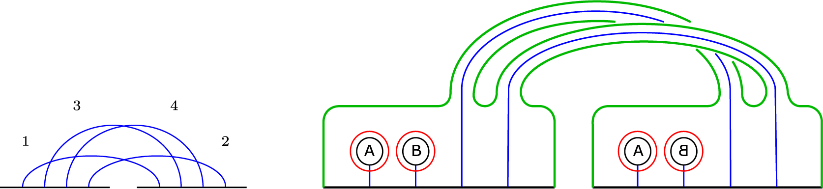
Figure 6.1 Left: The arc diagram for the torus example in Figure 3.1; note that the arc $e_i$
corresponding to
$e_i$
corresponding to $\delta _i$
is labelled with i. Right: The bordered sutured diagram
$\delta _i$
is labelled with i. Right: The bordered sutured diagram $\mathcal H^r$
for
$\mathcal H^r$
for $r=\{e_2,e_4\}$
.
$r=\{e_2,e_4\}$
.
We now consider a particular cap that arises naturally in the context of the bordered sutured manifold $(M,\mathsf {\Gamma },\mathcal {Z})$
associated to a foliated contact three-manifold
$(M,\mathsf {\Gamma },\mathcal {Z})$
associated to a foliated contact three-manifold $(M,\xi ,\mathcal {F})$
. As in Section 3.1, let
$(M,\xi ,\mathcal {F})$
. As in Section 3.1, let $\mathcal {Z}=(Z,a,m)$
be the arc diagram which parametrizes the bordered part
$\mathcal {Z}=(Z,a,m)$
be the arc diagram which parametrizes the bordered part $F=F(\mathcal {Z})$
in
$F=F(\mathcal {Z})$
in $\partial M$
and let
$\partial M$
and let $\Gamma (\mathcal {F})$
denote the dividing set associated to the foliation
$\Gamma (\mathcal {F})$
denote the dividing set associated to the foliation $\mathcal {F}$
. Let k be the number of elements in
$\mathcal {F}$
. Let k be the number of elements in $H_{\pm }$
, so
$H_{\pm }$
, so $|a|=4k$
. Each matched pair of points in a corresponds to a hyperbolic point and to a parameterizing arc
$|a|=4k$
. Each matched pair of points in a corresponds to a hyperbolic point and to a parameterizing arc $e_i\subset \delta _i$
, where
$e_i\subset \delta _i$
, where $i\in [2k]$
is the index of the point. From now on, fix
$i\in [2k]$
is the index of the point. From now on, fix $r=\amalg _{i\in H_{+}}e_i$
and define the associated cap
$r=\amalg _{i\in H_{+}}e_i$
and define the associated cap $\mathcal {W}:=\mathcal {W}_{r}$
with suture
$\mathcal {W}:=\mathcal {W}_{r}$
with suture $\mathsf {\Gamma }_{r}$
.
$\mathsf {\Gamma }_{r}$
.
Correspondingly, we define the sutured manifold $(M, \widetilde {\Gamma }):= (M,\mathsf {\Gamma },\mathcal {Z})\cup _{F}\mathcal {W}$
. We will show here that the sutures
$(M, \widetilde {\Gamma }):= (M,\mathsf {\Gamma },\mathcal {Z})\cup _{F}\mathcal {W}$
. We will show here that the sutures $\widetilde {\Gamma }$
may in fact be identified with
$\widetilde {\Gamma }$
may in fact be identified with $-\Gamma (\mathcal {F})$
. Recall that
$-\Gamma (\mathcal {F})$
. Recall that $\widetilde {\Gamma }$
separates
$\widetilde {\Gamma }$
separates $\partial M$
into regions
$\partial M$
into regions $R_\pm (\widetilde {\Gamma })$
. It is straightforward from the definition that
$R_\pm (\widetilde {\Gamma })$
. It is straightforward from the definition that
 $$\begin{align*}R_{-}(\widetilde{\Gamma})=R_{-}(\mathsf {\Gamma })\cup R_-(\mathsf {\Gamma }_r)=R_-(\mathsf {\Gamma })\bigcup(R\cup N(r)).\end{align*}$$
Observe that $R_-(\mathsf {\Gamma })\bigcup (R\cup N(r))$
is a neighborhood of the stable separatrices of points in
$R_-(\mathsf {\Gamma })\bigcup (R\cup N(r))$
is a neighborhood of the stable separatrices of points in $H_+$
. Thus, we can identify it with
$H_+$
. Thus, we can identify it with $R_+(\mathcal {F})$
, and as a consequence,
$R_+(\mathcal {F})$
, and as a consequence, $\widetilde {\Gamma }=-\partial R_+(\mathcal {F})$
and is isotopic to
$\widetilde {\Gamma }=-\partial R_+(\mathcal {F})$
and is isotopic to $-\Gamma (\mathcal {F})$
. To avoid a proliferation of notation, we will henceforth denote the sutured manifold obtained by gluing the cap as
$-\Gamma (\mathcal {F})$
. To avoid a proliferation of notation, we will henceforth denote the sutured manifold obtained by gluing the cap as $(M,\Gamma ):=(M, -\Gamma (\mathcal {F}))$
.
$(M,\Gamma ):=(M, -\Gamma (\mathcal {F}))$
.
Consequently, if we define $\overline {\mathcal {W}}=(-W,\mathsf {\Gamma },-\overline {\mathcal Z})$
, then
$\overline {\mathcal {W}}=(-W,\mathsf {\Gamma },-\overline {\mathcal Z})$
, then
 $$\begin{align*}(-M,-\Gamma(\mathcal{F}))=(-M,\mathsf {\Gamma },\overline{\mathcal Z})\cup_{\overline{F}} \overline{\mathcal{W}}.\end{align*}$$
The gluing formula gives the following:
 $$\begin{align*}\mathit{SFC}(-M,-\Gamma(\mathcal{F}))\simeq \widehat{\mathit{BSA}}(-M,\mathsf {\Gamma },\overline{\mathcal Z})\boxtimes_{\mathcal{A}(\overline{\mathcal Z})}\widehat{\mathit{BSD}}(\overline{\mathcal{W}}).\end{align*}$$
Let $\iota _r\in \mathcal {A}(\overline {\mathcal Z})$
be the idempotent corresponding to the horizontal arcs for the points in a that lie on the boundary of r. It follows from the special structure of the Heegaard diagram for
$\iota _r\in \mathcal {A}(\overline {\mathcal Z})$
be the idempotent corresponding to the horizontal arcs for the points in a that lie on the boundary of r. It follows from the special structure of the Heegaard diagram for $\mathcal {W}$
that
$\mathcal {W}$
that $\widehat {\mathit {BSD}}(\overline {\mathcal {W}})$
is an elementary type D module generated by
$\widehat {\mathit {BSD}}(\overline {\mathcal {W}})$
is an elementary type D module generated by $\iota _{r}$
; see [Reference ZarevZar10, Proposition 6.2]. Thus,
$\iota _{r}$
; see [Reference ZarevZar10, Proposition 6.2]. Thus,
 $$\begin{align*}\mathit{SFH}(-M,-\Gamma(\mathcal{F}))\cong H_*\left(\widehat{\mathit{BSA}}(-M,\mathsf {\Gamma },\overline{\mathcal Z})\right)\cdot \iota_r.\end{align*}$$
See [Reference ZarevZar10, Theorem 6.5].
We now prove Theorem 3 for $\iota _+$
given by
$\iota _+$
given by $\iota _r$
.
$\iota _r$
.
Proof of Theorem 3
Suppose $(\{S_i\}_{i=0}^{2k}, h, \{\gamma _i^{\pm }\})$
is a sorted foliated open book compatible with the triple
$(\{S_i\}_{i=0}^{2k}, h, \{\gamma _i^{\pm }\})$
is a sorted foliated open book compatible with the triple $(M,\xi ,\mathcal {F})$
. Let
$(M,\xi ,\mathcal {F})$
. Let $\mathcal {H}=(\Sigma ,{\boldsymbol {\alpha }},{\boldsymbol {\beta }}={\boldsymbol {\beta }}^a\cup {\boldsymbol {\beta }}^c,\mathcal Z)$
be the bordered sutured Heegaard diagram constructed in Section 3.2 for
$\mathcal {H}=(\Sigma ,{\boldsymbol {\alpha }},{\boldsymbol {\beta }}={\boldsymbol {\beta }}^a\cup {\boldsymbol {\beta }}^c,\mathcal Z)$
be the bordered sutured Heegaard diagram constructed in Section 3.2 for $(M,\mathsf {\Gamma }, \mathcal Z)$
. We begin with a brief sketch of the argument before presenting it in detail. First, we will construct a sutured Heegaard diagram for
$(M,\mathsf {\Gamma }, \mathcal Z)$
. We begin with a brief sketch of the argument before presenting it in detail. First, we will construct a sutured Heegaard diagram for $(M,-\Gamma (\mathcal {F}))$
by gluing
$(M,-\Gamma (\mathcal {F}))$
by gluing $\mathcal {H}$
to the diagram
$\mathcal {H}$
to the diagram $\mathcal {H}^{r}$
, where
$\mathcal {H}^{r}$
, where $\mathcal {H}^{r}$
denotes the diagram for the cap
$\mathcal {H}^{r}$
denotes the diagram for the cap $\mathcal {W}$
described above. Then, we show that after possibly performing some handleslides and
$\mathcal {W}$
described above. Then, we show that after possibly performing some handleslides and $2k$
-times destabilizing this diagram, one recovers the sutured Heegaard diagram corresponding to the partial open book
$2k$
-times destabilizing this diagram, one recovers the sutured Heegaard diagram corresponding to the partial open book $(S'=S_{0}, P'=P_{0},h'=h|_{P_{2k}}\circ \iota )$
compatible with the contact sutured manifold
$(S'=S_{0}, P'=P_{0},h'=h|_{P_{2k}}\circ \iota )$
compatible with the contact sutured manifold $(M,\Gamma (\mathcal {F}),\xi )$
, following the conventions in [Reference Honda, Kazez and MatićHKM09a, Section 2]. Note that this is a diagram for
$(M,\Gamma (\mathcal {F}),\xi )$
, following the conventions in [Reference Honda, Kazez and MatićHKM09a, Section 2]. Note that this is a diagram for $(M,-\Gamma (\mathcal {F}))$
. Letting
$(M,-\Gamma (\mathcal {F}))$
. Letting $\mathbf {x}^r=\{x_i^r\ |\ i\in H_-\}$
denote the generator of
$\mathbf {x}^r=\{x_i^r\ |\ i\in H_-\}$
denote the generator of $\mathcal {H}^r$
, we additionally prove that the map induced by the Heegaard moves sends the generator
$\mathcal {H}^r$
, we additionally prove that the map induced by the Heegaard moves sends the generator $\mathbf {x}\otimes \mathbf {x}^r$
in
$\mathbf {x}\otimes \mathbf {x}^r$
in $\mathit {SFC}(\overline {\mathcal {H}}\cup \overline {\mathcal {H}^r})$
to the generator which represents the contact invariant
$\mathit {SFC}(\overline {\mathcal {H}}\cup \overline {\mathcal {H}^r})$
to the generator which represents the contact invariant $\mathrm {EH}(M,\Gamma (\mathcal {F}), \xi )\in \mathit {SFH}(-M,-\Gamma (\mathcal {F}))$
.
$\mathrm {EH}(M,\Gamma (\mathcal {F}), \xi )\in \mathit {SFH}(-M,-\Gamma (\mathcal {F}))$
.
After gluing $\mathcal {H}$
and
$\mathcal {H}$
and $\mathcal {H}^r$
along Z, for every
$\mathcal {H}^r$
along Z, for every $i\in [2k]$
, the arc
$i\in [2k]$
, the arc $\beta _i^{r}$
in
$\beta _i^{r}$
in $\Sigma ^r$
will be paired with the arc
$\Sigma ^r$
will be paired with the arc $\beta _i^{a}$
in
$\beta _i^{a}$
in $\Sigma $
, producing a circle
$\Sigma $
, producing a circle $\widetilde {\beta }_i$
. For any
$\widetilde {\beta }_i$
. For any $i\in H_+$
, there exists a circle
$i\in H_+$
, there exists a circle $\widetilde {\alpha }_i$
in
$\widetilde {\alpha }_i$
in ${\boldsymbol {\alpha }}$
, and for any
${\boldsymbol {\alpha }}$
, and for any $i\in H_-$
, we define
$i\in H_-$
, we define $\widetilde {\alpha }_i=\alpha _i^{r}$
. We write
$\widetilde {\alpha }_i=\alpha _i^{r}$
. We write ${{\boldsymbol {\alpha }}}^r=\{\widetilde {\alpha }_i\ |\ i\in H_-\}$
. Then
${{\boldsymbol {\alpha }}}^r=\{\widetilde {\alpha }_i\ |\ i\in H_-\}$
. Then
 $$\begin{align*}\mathcal{H}'=\mathcal{H}\cup\mathcal{H}^{r}=\left(\Sigma'=\Sigma\cup_{Z}\Sigma^{r},{\boldsymbol{\alpha}}'={\boldsymbol{\alpha}}\cup{{\boldsymbol{\alpha}}}^r, {\boldsymbol{\beta}}'={\boldsymbol{\beta}}^c\cup\{\widetilde{\beta}_i\}_{i\in [2k]}\right) \end{align*}$$
is a Heegaard diagram for $(M,-\Gamma (\mathcal {F}))$
. In this diagram, we see that
$(M,-\Gamma (\mathcal {F}))$
. In this diagram, we see that $\widetilde {\alpha }_i\cap \widetilde {\beta }_i=\{x_i^{+}\}$
for
$\widetilde {\alpha }_i\cap \widetilde {\beta }_i=\{x_i^{+}\}$
for $i\in H_+$
, while
$i\in H_+$
, while $\widetilde {\alpha }_i\cap \widetilde {\beta }_i=\{x_i^{r}\}$
for
$\widetilde {\alpha }_i\cap \widetilde {\beta }_i=\{x_i^{r}\}$
for $i\in H_-$
. Furthermore, for
$i\in H_-$
. Furthermore, for $i\in H_-$
, the
$i\in H_-$
, the $\alpha $
-circle
$\alpha $
-circle $\widetilde {\alpha }_i$
is disjoint from all circles in
$\widetilde {\alpha }_i$
is disjoint from all circles in ${\boldsymbol {\beta }}'$
aside from
${\boldsymbol {\beta }}'$
aside from $\widetilde {\beta }_i$
. On the other hand, since
$\widetilde {\beta }_i$
. On the other hand, since $\mathcal H$
is defined using an abstract sorted foliated open book decomposition, Condition (2) of Definition 2.21 implies that, for any
$\mathcal H$
is defined using an abstract sorted foliated open book decomposition, Condition (2) of Definition 2.21 implies that, for any $i,j\in H_+$
, the arc
$i,j\in H_+$
, the arc $\beta _i^a\subset \Sigma $
is disjoint from the circle
$\beta _i^a\subset \Sigma $
is disjoint from the circle $\widetilde {\alpha }_j\subset \Sigma $
if and only if
$\widetilde {\alpha }_j\subset \Sigma $
if and only if $j>i$
. Thus, for
$j>i$
. Thus, for $i\in H_+$
, the
$i\in H_+$
, the $\beta $
-circle
$\beta $
-circle $\widetilde {\beta }_i$
is disjoint from the subset
$\widetilde {\beta }_i$
is disjoint from the subset
 $$\begin{align*}\{\alpha_1,\ldots,\alpha_{2g_0+n_0+|A_0|-k-2}\}\cup\{\widetilde{\alpha}_j\ |\ j\in H_+\ \text{and}\ j>i\}\cup{{\boldsymbol{\alpha}}}^r\subset{\boldsymbol{\alpha}}'.\end{align*}$$
Suppose $i\in H_-$
. Since
$i\in H_-$
. Since $\widetilde {\alpha }_i$
intersects
$\widetilde {\alpha }_i$
intersects $\widetilde {\beta }_i$
once, the curves in
$\widetilde {\beta }_i$
once, the curves in ${\boldsymbol {\alpha }}$
can be made disjoint from
${\boldsymbol {\alpha }}$
can be made disjoint from $\widetilde {\beta }_i$
by sliding each curve in
$\widetilde {\beta }_i$
by sliding each curve in ${\boldsymbol {\alpha }}$
that intersects
${\boldsymbol {\alpha }}$
that intersects $\widetilde {\beta }_i$
over
$\widetilde {\beta }_i$
over $\widetilde {\alpha }_i$
. Then we may destabilize
$\widetilde {\alpha }_i$
. Then we may destabilize $\mathcal {H}'$
using the pair
$\mathcal {H}'$
using the pair $\widetilde {\alpha }_i$
and
$\widetilde {\alpha }_i$
and $\widetilde {\beta }_i$
. Repeating this procedure for each
$\widetilde {\beta }_i$
. Repeating this procedure for each $i\in H_-$
yields a Heegaard diagram
$i\in H_-$
yields a Heegaard diagram $\mathcal H''=(\Sigma '',{\boldsymbol {\alpha }}'',{\boldsymbol {\beta }}'')$
for
$\mathcal H''=(\Sigma '',{\boldsymbol {\alpha }}'',{\boldsymbol {\beta }}'')$
for $(M,-\Gamma (\mathcal {F}))$
, where
$(M,-\Gamma (\mathcal {F}))$
, where ${\boldsymbol {\alpha }}''={\boldsymbol {\alpha }}$
,
${\boldsymbol {\alpha }}''={\boldsymbol {\alpha }}$
, ${\boldsymbol {\beta }}''={\boldsymbol {\beta }}^c\cup \{\widetilde {\beta }_i\}_{i\in H_+}$
, and
${\boldsymbol {\beta }}''={\boldsymbol {\beta }}^c\cup \{\widetilde {\beta }_i\}_{i\in H_+}$
, and $\Sigma ''$
is obtained from
$\Sigma ''$
is obtained from $\Sigma $
by attaching bands along
$\Sigma $
by attaching bands along $\partial \beta _i^a$
for each
$\partial \beta _i^a$
for each $i\in H_+$
.
$i\in H_+$
.
Write $H_-=\{j_1<j_2<\cdots <j_k\}$
. Let
$H_-=\{j_1<j_2<\cdots <j_k\}$
. Let $\mathcal {H}^{\prime }_l=(\Sigma ^{\prime }_l,{\boldsymbol {\alpha }}^{\prime }_l,{\boldsymbol {\beta }}^{\prime }_l)$
be the Heegaard diagram obtained from
$\mathcal {H}^{\prime }_l=(\Sigma ^{\prime }_l,{\boldsymbol {\alpha }}^{\prime }_l,{\boldsymbol {\beta }}^{\prime }_l)$
be the Heegaard diagram obtained from $\mathcal {H}'$
by applying the aforementioned Heegaard moves for
$\mathcal {H}'$
by applying the aforementioned Heegaard moves for $j_1,\ldots ,j_{l-1}$
. Denote by
$j_1,\ldots ,j_{l-1}$
. Denote by
 $$\begin{align*}f^-_{l}:\mathit{SFC}(\overline{\mathcal{H}'}_{l})=\mathit{SFC}(\Sigma^{\prime}_{l},{\boldsymbol{\beta}}^{\prime}_{l},{\boldsymbol{\alpha}}^{\prime}_{l})\to\mathit{SFC}(\overline{\mathcal{H}'}_{l+1})=\mathit{SFC}(\Sigma^{\prime}_{l+1},{\boldsymbol{\beta}}^{\prime}_{l+1},{\boldsymbol{\alpha}}^{\prime}_{l+1})\end{align*}$$
the composition of chain maps corresponding to the lth sequence of moves.
Let $f^-=f^-_{k}\circ \cdots \circ f^-_1$
. Note that the intersection points for
$f^-=f^-_{k}\circ \cdots \circ f^-_1$
. Note that the intersection points for $\mathcal {H}$
and
$\mathcal {H}$
and $\mathcal {H}''$
are in one-to-one correspondence, and
$\mathcal {H}''$
are in one-to-one correspondence, and $\mathbf {x}\in \mathit {SFC}(\overline {\mathcal {H}''})$
denotes the generator corresponding to the intersection point
$\mathbf {x}\in \mathit {SFC}(\overline {\mathcal {H}''})$
denotes the generator corresponding to the intersection point $\mathbf {x}$
for
$\mathbf {x}$
for $\mathcal {H}$
. Let
$\mathcal {H}$
. Let $f^h_l$
be the composition of chain maps associated with the sequence handleslides, and let
$f^h_l$
be the composition of chain maps associated with the sequence handleslides, and let $f_l^{ds}$
be the chain map associated with the subsequent destabilization. By an argument analogous to that in the proof of Proposition 4.5, we have that for an appropriate choice of the complex structure
$f_l^{ds}$
be the chain map associated with the subsequent destabilization. By an argument analogous to that in the proof of Proposition 4.5, we have that for an appropriate choice of the complex structure $f^-_l=f_l^{ds}\circ f_l^h(\mathbf {x}\otimes \mathbf {x}^{r}_l)=\mathbf {x}\otimes \mathbf {x}_{l+1}^{r}$
, and so
$f^-_l=f_l^{ds}\circ f_l^h(\mathbf {x}\otimes \mathbf {x}^{r}_l)=\mathbf {x}\otimes \mathbf {x}_{l+1}^{r}$
, and so $f^-(\mathbf {x}\otimes \mathbf {x}^{r})=\mathbf {x}$
. Here,
$f^-(\mathbf {x}\otimes \mathbf {x}^{r})=\mathbf {x}$
. Here, $\mathbf {x}_l^{r}=\{x_{j_i}^{r}\ |\ l\le i\le k\}$
.
$\mathbf {x}_l^{r}=\{x_{j_i}^{r}\ |\ l\le i\le k\}$
.
Next, we simplify the diagram $\mathcal {H}''$
using the pairs
$\mathcal {H}''$
using the pairs $\widetilde {\alpha }_i$
and
$\widetilde {\alpha }_i$
and $\widetilde {\beta }_i$
for all
$\widetilde {\beta }_i$
for all $i\in H_+$
. Suppose
$i\in H_+$
. Suppose $H_+=\{i_1<i_2 <\cdots <i_k\}$
. Note that
$H_+=\{i_1<i_2 <\cdots <i_k\}$
. Note that $\widetilde {\beta }_{i_1}\cap \widetilde {\alpha }_{i_1}=x^+_{i_1}$
while
$\widetilde {\beta }_{i_1}\cap \widetilde {\alpha }_{i_1}=x^+_{i_1}$
while $\widetilde {\beta }_{i_1}$
is disjoint from the rest of the
$\widetilde {\beta }_{i_1}$
is disjoint from the rest of the $\alpha $
-circles. As before, first slide every
$\alpha $
-circles. As before, first slide every $\beta $
-circle that intersects
$\beta $
-circle that intersects $\widetilde {\alpha }_{i_1}$
over
$\widetilde {\alpha }_{i_1}$
over $\widetilde {\beta }_{i_1}$
to remove the intersection points and then destabilize the diagram using
$\widetilde {\beta }_{i_1}$
to remove the intersection points and then destabilize the diagram using $\widetilde {\alpha }_{i_1}$
and
$\widetilde {\alpha }_{i_1}$
and $\widetilde {\beta }_{i_1}$
. In the new diagram,
$\widetilde {\beta }_{i_1}$
. In the new diagram, $\widetilde {\beta }_{i_2}$
is disjoint from all
$\widetilde {\beta }_{i_2}$
is disjoint from all $\alpha $
-circles except
$\alpha $
-circles except $\widetilde {\alpha }_{i_2}$
and
$\widetilde {\alpha }_{i_2}$
and $\widetilde {\beta }_{i_1}\cap \widetilde {\alpha }_{i_1}=x^+_{i_2}$
. So we can repeat this simplification for
$\widetilde {\beta }_{i_1}\cap \widetilde {\alpha }_{i_1}=x^+_{i_2}$
. So we can repeat this simplification for $i_2$
and in fact continue until
$i_2$
and in fact continue until $i=i_k$
. At the end, we get a surface homeomorphic to
$i=i_k$
. At the end, we get a surface homeomorphic to $\Sigma \setminus \amalg _{i\in H_+}N(\beta _i^a)$
. By definition,
$\Sigma \setminus \amalg _{i\in H_+}N(\beta _i^a)$
. By definition, $\Sigma =S_{\epsilon }\cup _B(-S_0)$
, where
$\Sigma =S_{\epsilon }\cup _B(-S_0)$
, where $S_{\epsilon }$
is a copy of
$S_{\epsilon }$
is a copy of $S_0$
. Therefore,
$S_0$
. Therefore,
 $$\begin{align*}\Sigma\setminus \amalg_{i\in H_+}N(\beta_i^a)\cong (S_{0}\setminus\amalg_{i\in H_+}N(\gamma_i^+))\cup_B(-S_0)=P_{0}\cup_{B}(-S_0)\end{align*}$$
and this surface is equipped with
 $$\begin{align*}\{\alpha_1,\ldots,\alpha_{2g_0+n_0+|A_0|-k-2} \}\quad \text{and} \quad\{\beta_1,\ldots,\beta_{2g_0+n_0+|A_0|-k-2}\}.\end{align*}$$
This is exactly the sutured Heegaard diagram defined in [Reference Honda, Kazez and MatićHKM09a] associated to the partial open book $(S',P',h')$
.
$(S',P',h')$
.
Let $\mathcal {H}^{\prime \prime }_l$
be the Heegaard diagram obtained from
$\mathcal {H}^{\prime \prime }_l$
be the Heegaard diagram obtained from $\mathcal {H}''$
after applying the above Heegaard moves for
$\mathcal {H}''$
after applying the above Heegaard moves for $i_1,\ldots ,i_{l-1}$
, and denote the chain map induced by the lth sequence of moves by
$i_1,\ldots ,i_{l-1}$
, and denote the chain map induced by the lth sequence of moves by
 $$\begin{align*}f_l^+:\mathit{SFC}(\overline{\mathcal{H}^{\prime\prime}_l})\to\mathit{SFC}(\overline{\mathcal{H}^{\prime\prime}_{l+1}}).\end{align*}$$
Let $f^+=f_k^+\circ \cdots \circ f_1^+$
. Once again, by an argument analogous to that in the proof of Proposition 4.5 we have that for an appropriate choice of complex structure,
$f^+=f_k^+\circ \cdots \circ f_1^+$
. Once again, by an argument analogous to that in the proof of Proposition 4.5 we have that for an appropriate choice of complex structure, $f^+(\mathbf {x})$
is the generator representing the contact invariant
$f^+(\mathbf {x})$
is the generator representing the contact invariant $\mathrm {EH}(M,\Gamma (\mathcal {F}),\xi )$
, that is,
$\mathrm {EH}(M,\Gamma (\mathcal {F}),\xi )$
, that is, $\{x_1,\ldots ,x_{2g_0+n_0+|A_0|-k-2}\}$
.
$\{x_1,\ldots ,x_{2g_0+n_0+|A_0|-k-2}\}$
.
Hence, $f^+_*\circ f^-_*(c_A(\xi )\cdot \iota _r)=f^+_*\circ f^-_*([\mathbf {x}\otimes \mathbf {x}^r])=\mathrm {EH}(M,\Gamma (\mathcal {F}),\xi )$
.
$f^+_*\circ f^-_*(c_A(\xi )\cdot \iota _r)=f^+_*\circ f^-_*([\mathbf {x}\otimes \mathbf {x}^r])=\mathrm {EH}(M,\Gamma (\mathcal {F}),\xi )$
.
7 Examples
Example 7.1. For our first example, consider the foliated open books obtained as follows. Begin with the open book for $(S^3, \xi _{\mathrm {std}})$
whose pages are disks. Embedding a sphere in this open book so that it intersects the binding in four points, as in Figure 7.1, produces two tight balls. See Figure 7.3. We first consider the ball whose initial page is a rectangle.
$(S^3, \xi _{\mathrm {std}})$
whose pages are disks. Embedding a sphere in this open book so that it intersects the binding in four points, as in Figure 7.1, produces two tight balls. See Figure 7.3. We first consider the ball whose initial page is a rectangle.

Figure 7.1 The sphere shown on the left separates $S^3$
into two tight balls and induces a foliated open book for each. The elliptic points are labelled with the signs associated to the ball whose first page is connected, as shown on the right.
$S^3$
into two tight balls and induces a foliated open book for each. The elliptic points are labelled with the signs associated to the ball whose first page is connected, as shown on the right.
Observe that this ball can also be obtained by cutting the solid torus of Example 2.5 along a meridional disk disjoint from the binding, which has the effect of removing a pair of hyperbolic points from the induced foliated open book. In this example, the first hyperbolic point is positive and the second negative, so the foliated open book is automatically sorted. The associated Heegaard diagram $\mathcal H_1$
is shown in Figure 7.2.
$\mathcal H_1$
is shown in Figure 7.2.

Figure 7.2 The bordered sutured Heegaard diagram adapted to the sorted foliated open book of Example 7.1.
Let x be the unique intersection point on the $S_{\epsilon }$
part of the diagram, and let y be the other intersection point. Let
$S_{\epsilon }$
part of the diagram, and let y be the other intersection point. Let $\rho _1$
and
$\rho _1$
and $\rho _2$
be the algebra elements corresponding to the Reeb chords on the inside and outside components of
$\rho _2$
be the algebra elements corresponding to the Reeb chords on the inside and outside components of $\partial \overline {\mathcal H_1}$
, as seen on Figure 7.2. The type A structure
$\partial \overline {\mathcal H_1}$
, as seen on Figure 7.2. The type A structure $\widehat {\mathit {BSA}}(\overline {\mathcal H_1})$
is generated by x and y, and has structure maps
$\widehat {\mathit {BSA}}(\overline {\mathcal H_1})$
is generated by x and y, and has structure maps
 $$ \begin{align*} m_2(y, \rho_1) & = x\\ m_2(y, \rho_2) & = x. \end{align*} $$
The contact class $c_A(B^3,\xi _1, \mathcal {F}_1)$
is the homotopy equivalence class of x.
$c_A(B^3,\xi _1, \mathcal {F}_1)$
is the homotopy equivalence class of x.
Example 7.2. As a second example we consider the ball in $(S^3, \xi _{\mathrm {std}})$
which is the complement of the previous example. See Figure 7.3.
$(S^3, \xi _{\mathrm {std}})$
which is the complement of the previous example. See Figure 7.3.

Observe that $S_0$
is disconnected, and the first negative hyperbolic point is followed by a second positive hyperbolic point. The associated foliated open book is not sorted, so we stabilize it before constructing the associated bordered sutured Heegaard diagram
$S_0$
is disconnected, and the first negative hyperbolic point is followed by a second positive hyperbolic point. The associated foliated open book is not sorted, so we stabilize it before constructing the associated bordered sutured Heegaard diagram $\mathcal H_2$
. The result of the stabilization is shown in Figure 7.4.
$\mathcal H_2$
. The result of the stabilization is shown in Figure 7.4.

Figure 7.4 A sorted foliated open book for the ball of Example 7.2.
By keeping track of the four elliptic points in the embedded open book decomposition of $(S^3, \xi _{\mathrm {std}})$
and their images on the two Heegaard diagrams, we see that the corresponding Heegaard diagram
$(S^3, \xi _{\mathrm {std}})$
and their images on the two Heegaard diagrams, we see that the corresponding Heegaard diagram $\mathcal H$
for
$\mathcal H$
for $(S^3, \xi _{\mathrm {std}})$
is obtained by gluing
$(S^3, \xi _{\mathrm {std}})$
is obtained by gluing $\mathcal H_1$
to
$\mathcal H_1$
to $\mathcal H_2$
by identifying the outside boundary component of one diagram to the inside boundary component of the other, and vice versa. Thus, to have consistent labels (between
$\mathcal H_2$
by identifying the outside boundary component of one diagram to the inside boundary component of the other, and vice versa. Thus, to have consistent labels (between $\mathcal H_1$
and
$\mathcal H_1$
and $\mathcal H_2$
) of the algebra generators for the given foliation, we must label the generator for the inside boundary component of
$\mathcal H_2$
) of the algebra generators for the given foliation, we must label the generator for the inside boundary component of $\overline {\mathcal H_2}$
by
$\overline {\mathcal H_2}$
by $\rho _2$
and the other one by
$\rho _2$
and the other one by $\rho _1$
. Let s be the unique intersection point on the
$\rho _1$
. Let s be the unique intersection point on the $S_{\epsilon }$
part of
$S_{\epsilon }$
part of $\overline {\mathcal H_2}$
, and let t be the other intersection point. The type D structure
$\overline {\mathcal H_2}$
, and let t be the other intersection point. The type D structure $\widehat {\mathit {BSD}}(\overline {\mathcal H_2})$
is generated by s and t, and has structure map
$\widehat {\mathit {BSD}}(\overline {\mathcal H_2})$
is generated by s and t, and has structure map
 $$\begin{align*}\delta^1(t) = (\rho_1+\rho_2)\otimes s.\\[-15pt]\end{align*}$$
The contact class $c_D(B^3,\xi _2, \mathcal {F}_2)$
is the homotopy equivalence class of s.
$c_D(B^3,\xi _2, \mathcal {F}_2)$
is the homotopy equivalence class of s.
Example 7.3. We take the box tensor product of the type A structure from Example 7.1 and the type D structure from Example 7.2, to compute the contact class for $(S^3, \xi _{\mathrm {std}})$
. Considering the idempotents,
$(S^3, \xi _{\mathrm {std}})$
. Considering the idempotents, $\widehat {\mathit {BSA}}(\overline {\mathcal {H}_1})\boxtimes \widehat {\mathit {BSD}}(\overline {\mathcal {H}_2})$
is generated by
$\widehat {\mathit {BSA}}(\overline {\mathcal {H}_1})\boxtimes \widehat {\mathit {BSD}}(\overline {\mathcal {H}_2})$
is generated by $y\otimes t$
and
$y\otimes t$
and $x\otimes s$
.The differential
$x\otimes s$
.The differential $\partial =\partial ^{\boxtimes }$
is trivial, so the homology
$\partial =\partial ^{\boxtimes }$
is trivial, so the homology $H_{\ast }(\widehat {\mathit {BSA}}(\overline {\mathcal {H}_1})\boxtimes \widehat {\mathit {BSD}}(\overline {\mathcal {H}_2}))$
is generated by
$H_{\ast }(\widehat {\mathit {BSA}}(\overline {\mathcal {H}_1})\boxtimes \widehat {\mathit {BSD}}(\overline {\mathcal {H}_2}))$
is generated by $[y\otimes t]$
and
$[y\otimes t]$
and $[x\otimes s]$
. Therefore,
$[x\otimes s]$
. Therefore, $[x\otimes s]$
is the contact class of the glued three-sphere
$[x\otimes s]$
is the contact class of the glued three-sphere $(S^3, \xi _{\mathrm {std}})$
.
$(S^3, \xi _{\mathrm {std}})$
.
Example 7.4. Finally, we return to the the running example used throughout this paper: the solid torus first introduced in Example 2.5. Recall that Example 3.3 constructed the bordered sutured Heegaard diagram adapted to a sorted foliated open book for this manifold. Here, we compute the associated type A structure.
For simplicity, we label the intersection points in Heegaard diagram $\mathcal H$
by
$\mathcal H$
by $x_1$
,
$x_1$
, $x_2$
,
$x_2$
, $x_3$
,
$x_3$
, $x_4$
,
$x_4$
, $y_1$
, and
$y_1$
, and $y_2$
as in Figure 7.5. In this diagram, we have six generators
$y_2$
as in Figure 7.5. In this diagram, we have six generators
 $$\begin{align*}\left\{x_1y_1, x_1y_2, x_2y_2,x_3y_1,x_3y_2,x_4y_2\right\}\end{align*}$$
where $x_1y_1$
is the generator
$x_1y_1$
is the generator $x_1^+x_3^+$
defined in Section 3.2. Then, we simplify our depiction of the Heegaard diagram
$x_1^+x_3^+$
defined in Section 3.2. Then, we simplify our depiction of the Heegaard diagram $\mathcal H$
by first removing the domains adjacent to
$\mathcal H$
by first removing the domains adjacent to $\partial \Sigma \setminus Z$
and then cutting along the intersection points
$\partial \Sigma \setminus Z$
and then cutting along the intersection points $x_1$
,
$x_1$
, $y_1$
and
$y_1$
and $y_2$
. Moreover,
$y_2$
. Moreover, $\overline {\mathcal H}$
is obtained from
$\overline {\mathcal H}$
is obtained from $\mathcal H$
by switching
$\mathcal H$
by switching ${\boldsymbol {\alpha }}$
and
${\boldsymbol {\alpha }}$
and ${\boldsymbol {\beta }}$
, so we draw
${\boldsymbol {\beta }}$
, so we draw ${\boldsymbol {\beta }}$
arcs in red and
${\boldsymbol {\beta }}$
arcs in red and ${\boldsymbol {\alpha }}$
circles in blue. See Figure 7.6.
${\boldsymbol {\alpha }}$
circles in blue. See Figure 7.6.
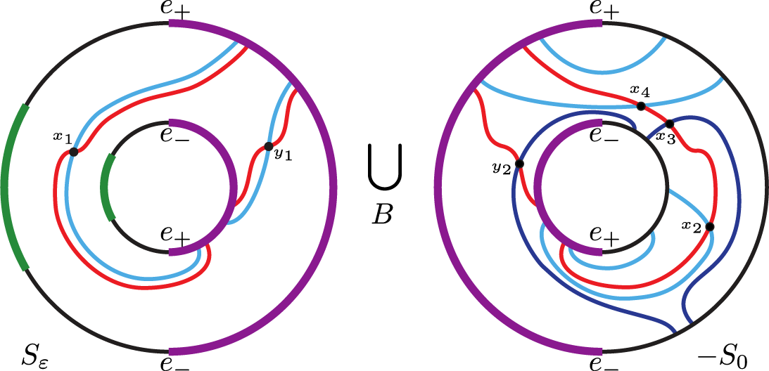
Figure 7.5 The Heegaard diagram $\mathcal {H}$
from Example 3.3, with intersection points labelled so that
$\mathcal {H}$
from Example 3.3, with intersection points labelled so that $x_1y_1$
is the contact class.
$x_1y_1$
is the contact class.

Figure 7.6 The portion of the Heegaard diagram $\mathcal H$
from Figure 7.5 relevant to the computation of
$\mathcal H$
from Figure 7.5 relevant to the computation of $\widehat {\mathit {BSA}}(\overline {\mathcal H})$
. The boundary is parametrized by an arc diagram which consists of two arcs with eight points on them. The intervals between points are labeled with
$\widehat {\mathit {BSA}}(\overline {\mathcal H})$
. The boundary is parametrized by an arc diagram which consists of two arcs with eight points on them. The intervals between points are labeled with $\{1,\ldots ,6\}$
in gray.
$\{1,\ldots ,6\}$
in gray.
Every region is adjacent to the boundary, so $m_1=0$
. We computed
$m_1=0$
. We computed $m_i$
for
$m_i$
for $i>1$
, by finding the local coefficients of curves and computing their Maslov indices. Then, it is easy to see that the curves with Maslov index one contribute to the maps listed below. Moreover,
$i>1$
, by finding the local coefficients of curves and computing their Maslov indices. Then, it is easy to see that the curves with Maslov index one contribute to the maps listed below. Moreover, $m_i=0$
for
$m_i=0$
for $i>3$
. Note that instead of
$i>3$
. Note that instead of
 $$\begin{align*}m_2(x_3y_2,I_{\{2,4\}}a(\{1,5\}))=x_3y_1\end{align*}$$
we write simply
 $$\begin{align*}m_2(x_3y_2,\{1,5\})=x_3y_1,\end{align*}$$
as the appropriate completion of a set of Reeb chords is clear from the context. The nontrivial maps are as follows.
 $$ \begin{align*} &m_2(x_3y_2, 5)=x_4y_2\\ &m_2(x_3y_2,\{1,5\})=x_3y_1\\ &m_2(x_3y_2,\{2,4\})=x_3y_1\\ &m_2(x_3y_2,2)=x_2y_2\\ &m_2(x_3y_2,23)=x_1y_2\\ &m_2(x_3y_2,56)=x_1y_2\\ &m_2(x_3y_2,\{123,5\})=x_1y_1\\ &m_2(x_3y_2,\{2,456\})=x_1y_1\\ &m_2(x_4y_2,123)=x_1y_1\\ &m_2(x_4y_2,1)=x_3y_1\\ &m_2(x_4y_2,6)=x_1y_2\\ &m_2(x_2y_2,4)=x_3y_1\\ &m_2(x_2y_2,456)=x_1y_1\\ &m_2(x_2y_2,3)=x_1y_2\\ &m_2(x_3y_1,23)=x_1y_1\\ &m_2(x_3y_1,56)=x_1y_1\\ &m_3(x_4y_2,\{1,6\},5)=x_1y_1\\ &m_3(x_4y_2,1,\{5,6\})=x_1y_1\\ &m_3(x_4y_2,\{4,6\},2)=x_1y_1\\ &m_3(x_4y_2,4,\{2,6\})=x_1y_1\\ &m_3(x_1y_2,1,5)=x_1y_1\\ &m_3(x_1y_2,4,2)=x_1y_1\\ &m_3(x_2y_2,4,\{2,3\})=x_1y_1\\ &m_3(x_2y_2,\{3,4\},2)=x_1y_1\\ &m_3(x_2y_2,1,\{3,5\})=x_1y_1\\ &m_3(x_2y_2,\{1,3\},5)=x_1y_1\\ &m_3(x_3y_2,\{1,23\},5)=x_1y_1\\ &m_3(x_3y_2,\{4,56\},2)=x_1y_1\\ &m_3(x_3y_2,\{4,23\},2)=x_1y_1\\ &m_3(x_3y_2,\{1,56\},5)=x_1y_1\\ &m_3(x_3y_2,\{1,2\},\{3,5\})=x_1y_1\\ &m_3(x_3y_2,\{4,5\},\{2,6\})=x_1y_1\\ &m_3(x_3y_2,\{2,4\},\{2,3\})=x_1y_1\\ &m_3(x_3y_2,\{1,5\},\{5,6\})=x_1y_1 \end{align*} $$
Example 7.5. Our next example is the solid torus in $(S^3, \xi _{\mathrm {std}})$
which is the complement of the previous example. As in Example 7.2, the embedded foliated open book arising from the disk open book for
$(S^3, \xi _{\mathrm {std}})$
which is the complement of the previous example. As in Example 7.2, the embedded foliated open book arising from the disk open book for $(S^3, \xi _{\mathrm {std}})$
is not sorted. A sequence of two stabilizations results in a sorted foliated open book, the first and last page of which are shown in Figure 7.7.
$(S^3, \xi _{\mathrm {std}})$
is not sorted. A sequence of two stabilizations results in a sorted foliated open book, the first and last page of which are shown in Figure 7.7.
The construction from Section 3.2 yields the Heegaard diagram $\mathcal H'$
shown in Figure 7.8.
$\mathcal H'$
shown in Figure 7.8.

Figure 7.7 The first and last page of a sorted foliated open book for the solid torus of Example 7.5.

Figure 7.8 The bordered sutured Heegaard diagram $\mathcal H'$
adapted to the sorted foliated open book depicted in Figure 7.7.
$\mathcal H'$
adapted to the sorted foliated open book depicted in Figure 7.7.
We label the intersection points in Heegaard diagram $\mathcal H'$
by
$\mathcal H'$
by $x_1'$
,
$x_1'$
, $x_2'$
,
$x_2'$
, $x_3'$
,
$x_3'$
, $x_4'$
,
$x_4'$
, $x_5'$
,
$x_5'$
, $x_6'$
,
$x_6'$
, $y_1'$
, and
$y_1'$
, and $y_2'$
as in Figure 7.8. We have eight generators
$y_2'$
as in Figure 7.8. We have eight generators
 $$\begin{align*}\left\{x_1'y_1', x_1'y_2', x_2'y_2',x_3'y_1',x_4'y_1',x_4'y_2', x_5'y_1', x_6'y_2'\right\},\end{align*}$$
where $x_1'y_1'$
is the generator
$x_1'y_1'$
is the generator $x_2^+x_4^+$
defined in Section 3.2. By removing the domains adjacent to
$x_2^+x_4^+$
defined in Section 3.2. By removing the domains adjacent to $\partial \Sigma \setminus Z$
and then cutting along the points
$\partial \Sigma \setminus Z$
and then cutting along the points $x_1', x_4', y_1'$
and
$x_1', x_4', y_1'$
and $y_2'$
we get the planar depiction of the Heegaard diagram
$y_2'$
we get the planar depiction of the Heegaard diagram $\mathcal H'$
shown in Figure 7.9. By matching elliptic points again, as in Example 7.2, we obtain labels
$\mathcal H'$
shown in Figure 7.9. By matching elliptic points again, as in Example 7.2, we obtain labels $\{1, \ldots , 6\}$
on the intervals of the arc diagram for
$\{1, \ldots , 6\}$
on the intervals of the arc diagram for $\mathcal H'$
consistent with those for the diagram
$\mathcal H'$
consistent with those for the diagram $\mathcal H$
from Example 7.4.
$\mathcal H$
from Example 7.4.

Figure 7.9 The portion of the Heegaard diagram $\mathcal H'$
from Figure 7.8 relevant to the computation of
$\mathcal H'$
from Figure 7.8 relevant to the computation of $\widehat {\mathit {BSD}}(\overline {\mathcal H'})$
.
$\widehat {\mathit {BSD}}(\overline {\mathcal H'})$
.
This time, we have a nice diagram, and the type D structure is straightforward to compute. The type D structure maps are listed below.
 $$ \begin{align*} \delta^1(x_1'y_1') &= 0\\ \delta^1(x_1'y_2') &= 2\otimes x_1'y_1' + 5\otimes x_1'y_1'\\ \delta^1(x_2'y_2') &= I\otimes x_3'y_1' + 1\otimes x_1'y_2'\\ \delta^1(x_3'y_1') &= 12\otimes x_1'y_1' \\ \delta^1(x_4'y_1') &= 123\otimes x_1'y_1' + 456\otimes x_1'y_1' + 3\otimes x_3'y_1' + 6\otimes x_5'y_1'\\ \delta^1(x_4'y_2') &= 123\otimes x_1'y_2' + 456\otimes x_1'y_2' + 23\otimes x_2'y_2' + 2\otimes x_4'y_1' + 5\otimes x_4'y_1' + 56\otimes x_6'y_2'\\ \delta^1(x_5'y_1') &= 45\otimes x_1'y_1' \\ \delta^1(x_6'y_2') &= 4\otimes x_1'y_2' + I\otimes x_5'y_1' \end{align*} $$
Example 7.6. We take the box tensor product of the type A structure from Example 7.4 and the type D structure from Example 7.5 to compute the contact class for $(S^3, \xi _{\mathrm {std}})$
.
$(S^3, \xi _{\mathrm {std}})$
.
Considering the idempotents, $\widehat {\mathit {BSA}}(\overline {\mathcal {H}})\boxtimes \widehat {\mathit {BSD}}(\overline {\mathcal {H}'})$
has
$\widehat {\mathit {BSA}}(\overline {\mathcal {H}})\boxtimes \widehat {\mathit {BSD}}(\overline {\mathcal {H}'})$
has $8$
generators:
$8$
generators:
 $$ \begin{align*} \left\{\begin{array}{l}x_1y_1\otimes x_1'y_1',\ x_1y_2\otimes x_2'y_2',\ x_1y_2\otimes x_3'y_1',\ x_1y_2\otimes x_5'y_1'\\x_1y_2\otimes x_6'y_2',\ x_2y_2\otimes x_4'y_1',\ x_3y_2\otimes x_4'y_2',\ x_4y_2\otimes x_4'y_1'\end{array}\right\}. \end{align*} $$
Moreover, the differential $\partial =\partial ^{\boxtimes }$
is given as follows:
$\partial =\partial ^{\boxtimes }$
is given as follows:
 $$ \begin{align*} \partial\left(x_3y_2\otimes x_4'y_2'\right)&=x_2y_2\otimes x_4'y_1'+x_4y_2\otimes x_4'y_1'+x_1y_2\otimes x_2'y_2'+x_1y_2\otimes x_6'y_2'\\ \partial\left(x_2y_2\otimes x_4'y_1' \right)&=x_1y_2\otimes x_3'y_1'+x_1y_1\otimes x_1'y_1'\\ \partial\left(x_4y_2\otimes x_4'y_1'\right)&=x_1y_2\otimes x_5'y_1'+x_1y_1\otimes x_1'y_1'\\ \partial\left(x_1y_2\otimes x_2'y_2'\right)&=x_1y_2\otimes x_3'y_1'+x_1y_1\otimes x_1'y_1'\\ \partial\left(x_1y_2\otimes x_6'y_2'\right)&=x_1y_2\otimes x_5'y_1'+x_1y_1\otimes x_1'y_1' \end{align*} $$
It is easy to see that the homology is generated by $[x_1y_1\otimes x_1'y_1']$
and
$[x_1y_1\otimes x_1'y_1']$
and $[x_1y_2\otimes x_2'y_2'+x_2y_2\otimes x_4'y_1']$
. Therefore,
$[x_1y_2\otimes x_2'y_2'+x_2y_2\otimes x_4'y_1']$
. Therefore, $[x_1y_1\otimes x_1'y_1']$
is the contact class
$[x_1y_1\otimes x_1'y_1']$
is the contact class $(S^3, \xi _{\mathrm {std}})$
. Observe that this agrees with the result in Example 7.3.
$(S^3, \xi _{\mathrm {std}})$
. Observe that this agrees with the result in Example 7.3.
Acknowledgements
This material is partially based upon work supported by the National Science Foundation under Grant DMS-1439786 while the authors were in residence at the Institute for Computational and Experimental Research in Mathematics in Providence, RI, during the Women in Symplectic and Contact Geometry and Topology workshop.
JEL would like to express her appreciation to the Australian Mathematical Society for their support in the form of an Anne Penfold Street Award. During the first six months of working on this paper, VV had a position at the University of Strasbourg with the CNRS; VV is grateful to both for providing a calm yet active research environment.
We thank Robert Lipshitz and Paolo Ghiggini for helpful conversations. We are also grateful to both of the anonymous referees for their careful reading and thoughtful comments.
Conflicts of Interest
The authors have no conflict of interest to declare.
Funding statement
AA was supported by NSF Grant DMS-2019396. VF was supported by the NKFIH Élvonal (Frontier) project KKP126683 and the National Talent Program NTP-NFTÖ-21. KH was supported by NSF CAREER Grant DMS-2019396 and a Sloan Research Fellowship. IP was supported by NSF Grant DMS-1711100. VV was supported by the ANR grant ‘Quantum topology and contact geometry’ and FWF grant P 34318.


 Open access