Introduction

During the Expédition Glaciologique Internationale au Groenland (E.G.I.G.) in 1959 and the U.S. Antarctic Research Programs in 1961–62 and 1962–63, several D.C. electrical resistivity measurements were made on the Greenland Ice Sheet and in Antarctica on the small ice cap of Roosevelt Island and on the Ross Ice Shelf. These measurements were made in order to study the variation of the specific resistivity with depth and to investigate the existence of low resistivity layers at the bottom of the ice sheet.

Method

The Schlumberger electrode configuration was used throughout the investigations. In making the measurements, the current I was limited to 1–2 mA. by the available voltage sources and a combined contact resistance of about 1−2 MΩ. at the current electrodes. Because of these limitations and low resistivities at depth, the electrode spacing L/2 could only be increased to about 1.5 km. before the potential drop ΔV could no longer be measured accurately above the background of extraneous potential changes at the potential electrodes.

Standard graphs and auxiliary diagrams given by CGG (1955) and Reference Buchheim and HaalckBuchheim (1958) were used for interpretation of the data. One graph was computed according to a theorem of Reference FlatheFlathe (1955).

Background

By 1961 it was known that there must exist two different ranges of resistivity for glacier ice:

Locally resistivities between 1 and 2 MΩ.m. can be found on cold glaciers and thin ice shelves, as reported by Reference Meyer and RöthlisbergerMeyer and Röthlisberger (1962) and by Vögtli (Reference ApollonioApollonio and others, 1961). Cold ice with similarly high resistivity was found on the Ross Ice Shelf near McMurdo Sound (Antarctica) by Reference Robertson and MacdonaldRobertson and Macdonald (1962). In the same area in 1961, the author measured a resistivity of 1.7 MΩ.m. in ice warmer than −20°C.

On the cold névé of continental ice sheets resistivity is a function of depth. The 1959 measurements on the Greenland Ice Sheet (Reference HochsteinHochstein, 1965) showed that the resistivity decreased sharply, reaching an unexpectedly low value of less than 0.1 MΩ.m.at an electrode spacing of L/2 = 600 m. At greater spacings, ρ _a remained nearly constant (Fig. 1). If the decrease of resistivity is an effect of densification, it should also be found in cores. Reference KoppKopp (1962) investigated the resistivity of some cores taken by the glaciological party of E.G.I.G. near “Station Dumont” (Greenland), but found no relation between the density γ and the resistivity ρ. Furthermore, the resistivities of the cores were 10–100 times greater than values obtained from field measurements. Samples of fresh compressed snow, however, showed a linear variation of log (ρ _i/ρ) with γ where ρ _i is the initial resistivity. Kopp also showed that the resistivity of firn cores and compressed snow samples was affected by the temperature, following the same law as the resistivity of pure ice:

where ρ _c is a constant, T the absolute temperature,

the activation energy, and k Boltzmann’s constant (8.62×10⁻⁵ eV./°C. = 1.98 cal./mole °C.). In all cases the activation energy for snow and firn was greater than the activation energy of pure ice.

Fig. 1. Apparent resistivity curve at “Station Centrale” (calculated resistivity-depth column is shown in the upper part of the figure; crosses indicate the origin of the applied model curves)

In 1961–62, resistivity measurements with short spreads were made on the top and at the border of the Roosevelt Island ice cap in order to determine if horizontal strain could affect resistivity. The temperature at a depth of 10 m. was about the same in both locations. No measurable effect could be observed. In 1962–63 resistivity measurements on Roosevelt Island were made with long profiles (electrode distances up to L/2 = 1.6 km.) on the top of the island and on the ice shelf near the margin of the island. The apparent resistivity curves (Figs. 2 and 3) show the expected decrease at shorter spreads. On the ice cap the apparent resistivity reached a minimum at L/2 = 1,000 m. with ρ _a=0.12 MΩ.m. and then increased, whereas on the ice shelf the resistivity decreased continuously. During the same season, the influence of densification upon resistivity was studied by measuring the resistivity in cores from a 15 m. drill hole.

Fig. 2. Apparent resistivity curve at “Camp Wisconsin” on Roosevelt Island

Fig. 3. Apparent resistivity curve on the Ross Ice Shelf near Roosevelt Island

The Resistivity of Firn and Ice on Ice Sheets

From earlier measurements, we can draw the conclusion that the resistivity of sedimentary ice is a function of (1) the “base” resistivity, (2) the contact resistance between the grains, (3) the temperature. Other factors, such as the past history of the ice, may also be important but will not be discussed for lack of information.

(1) According to recent theories (Reference JaccardJaccard, 1959; Reference GränicherGränicher, 1958) the conductivity of pure ice results from the presence of OH⁻ and H₃O⁺ ions together with lattice defects.

In order to explain the difference in resistivity between cold and temperate glacier ice it was first thought that the resistivity of sedimentary ice is generally lowered by chemical impurities (i.e. electrolytic conductivity) and that a different distribution of these impurities may cause the difference in resistivity. But in the case of electrolytic conductivity the activation energy

of sedimentary ice should be smaller than measured; besides, near the freezing point of the “ice-electrolyte” a jump of resistivity should occur which was not observed (Reference HochsteinHochstein, 1965).

If the conductivity of sedimentary ice results from chemical and lattice defects a different production of these defects can be responsible for the observed various resistivities. Recrystallization—which is the main difference between cold and temperate glacier ice—could affect the equilibrium of the defects. Laboratory measurements by Reference KoppKopp (1962) indeed show an increase of the resistivity of compressed snow during recrystallization. Field measurements on the other hand give evidence of a layer with high resistivity at the bottom of cold glaciers in North Greenland and at the bottom of the ice sheet near the coast in mid Greenland (Reference Meyer and RöthlisbergerMeyer and Röthlisberger, 1962; Reference HochsteinHochstein, 1965) and since recrystallization should only occur at the bottom of ice sheets the field results also support the conclusion that apparently the difference of resistivity between cold and temperate glacier ice is related to the rate of recrystallization.

(2) In firn and ice, resistivity also depends upon the contact resistance between the grains which is a function of grain size and pressure. With increasing grain size and increasing pressure the contact area between grains must become larger, the contact resistance consequently must decrease.

The resistivity measurements in Greenland during E.G.I.G. suggested that densification has an influence upon resistivity. Laboratory measurements made by Reference KoppKopp (1962) gave proof for compressed snow samples; between the available density range 0.2 g./cm.³ < γ < 0.6 g./cm.³ the variation of resistivity could be described by:

The coefficient in the exponent was affected by the grain size. Kopp got the values −12.3 for fresh snow, −9.1 for powder snow, and −3.9 for granulated snow (transforming his graphs of log (ρ _i/ρ) versus γ into ρ = a exp (b γ)). But resistivities of firn cores from Greenland scattered over a broad range and did not show a relationship between resistivity and density.

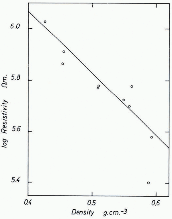
In order to check the influence of densification we measured resistivity and density of core samples directly in the field during the 1962/63 season at “Camp Wisconsin” on Roosevelt Island (lat. 79° 16′ S.; long. 162° 15′ W., elevation 560 m., accumulation ≃ 16 g./cm.² yr., 10-metre temperature −23.0°C.). Since the work was done in a 3 m. pit the temperature t of the cores did not change more than 1 or 2°C. from −22°C. during the measurements (t will be used throughout for Centigrade temperatures). Resistivity and density were measured immediately after drilling. The cores were stored in the pit and some remeasured after one and a half months, but no significant difference could be found. Brass plates frozen to the ends of the cores were used as electrodes. The resistance R was measured with a Keithley electrometer (model 610 A) and the resistivity calculated from: ρ = Rq/l, where q is the cross-sectional area and l the length of the core. The experimental error of these measurements was about 10–25 per cent due to uncertainty about contact resistance (about 2 MΩ.), anisotropy, and polarity. The field strength in the cores did not exceed 2 V./cm. We found that the average resistivity (over 1 m. length) decreased from 1.05 MΩ.m. (γ =0.426 g./cm.³) at 2.5 m. depth to 0.38 MΩ.m. (γ = 0.593 g./cm.³) at 14.5 m. depth. Plotting log ρ against γ (Fig. 4a), we see that between γ = 0.35 g./cm.³ and γ = 0.60 g./cm.³ the resistivity approximately follows the equation:

Fig. 4a. Variation of resistivity with density on Roosevelt Island

Assuming that the density on the island is constant (γ = 0.9 g./cm.³) at a depth greater than 100 m. (the temperature at this depth is still about −22°C. anticipating results shown at the end of the paper) from Equation (2a) we get a resistivity of ρ = 0.085 MΩ.m. The interpretation of the resistivity curve (Fig. 2) shows, however, that the resistivity around 100 m. depth is still about 0.19 MΩ.m. Equation (2) seems, therefore, only applicable to a limited range of density and thus γ is not an appropriate parameter to describe the variation of resistivity with depth.Footnote *

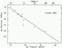
As the next step we tried to correlate resistivity and hydrostatic pressure. Assuming that the contact resistance of the grains inside the cores will not change if the pressure is removed by drilling, we can plot log ρ versus log p at the depth z where the pressure

(Fig. 4b). In this plot the points indicate a linear relation, i.e. explicitly a function of the type:

where ρ′_c and x are constants. In addition to the directly measured resistivities the interpretation of the resistivity curve at “Camp Wisconsin” (Fig. 2) yields average resistivities for the second and third layers of ρ ₂ = 0.22 MΩ.m. and ρ ₃ = 0.165 MΩ.m. at average depths of z ₂ = 58.5 m. and z ₃ = 250 m. The temperature at these depths (−23°C. < t <−21°C.) is about the same as the temperature of the cores. Therefore we can plot these values also in Figure 4b where they match the linear function fairly well. A least-squares fit of the constants gives the equation:

where p is the hydrostatic pressure in kg./cm.². According to (3a) the variation of resistivity due to increasing pressure is small at greater depths. At “Camp Wisconsin” for example the resistivity is lowered about 20 per cent between 250 m. and 500 m. and about 14 per cent between 500 m. and 750 m.

Fig. 4b. Variation of resistivity with hydrostatic pressure on Roosevelt Island. Measured (averaged) resistivities on core samples are marked with circles, crosses indicate calculated resistivities from the apparent resistivity curve

(3) The resistivity of pure and sedimentary ice is affected by the temperature, following the law of Arrhenius given in equation (1). The activation energy

of pure ice according to Reference JaccardJaccard (1959) is about 0.61 eV. Reference KoppKopp (1962) found values of . in snow samples and . in firn samples.

For a detailed interpretation of resistivity curves on ice sheets, the exact value of the activation energy is important. Comparison of parallel resistivity curves provides a first check on

.

In Greenland the resistivity curves of “Station Centrale” and “Point Nord” are nearly parallel up to L/2 = 400 m., the ratio of the apparent resistivities is about 1.5 : 1 to 2 : 1 and the temperature about −28°C. at “Station Centrale” and −21°C. at “Point Nord”. These temperatures are constant at least up to a depth of 300 m. Assuming the same structure and density gradient, we get from equation (1) a value of 0.3 to 0.55 eV. for the activation energy (Reference HochsteinHochstein, 1965).

The resistivity curves from Roosevelt Island and the Ross Ice Shelf (Figs. 2 and 3) are also nearly parallel up to L/2 = 60 m. The 10 m. temperatures at these two locations are −23°C. and −26°C., the ratio of the apparent resistivities is about 0.8 : 1 which yield for

a value of 0.35 eV.

An average value of

at greater depths can be derived from a single resistivity curve if at two different depths z ₁, and z ₂ the corresponding resistivities ρ ₁ and ρ ₂ and temperatures t ₁ and t ₂ are known.

On the ice shelf near Roosevelt Island interpretation of the apparent resistivity curve (Fig. 3) gave the following values: at 10 m. depth ρ ₁ was about 0.65 MΩ.m., while at the bottom of the floating ice shelf at 500 m. depth ρ ₂ was about 0.02 to 0.035 MΩ.m. The temperature at these depths were about T ₁=26°C. and T ₂ = −2°C. If we consider the influence of hydrostatic pressure according to equation (3a) the resistivity ρ ₁ would be lowered to about 0.135 MΩ.m. at 500 m. depth. From equation (1) the corresponding activation energy is 0.38±0.1 eV. This figure agrees with the value of

. derived from parallel curves.Footnote *

The variation of resistivity with temperature is nearly the same in Greenland and Antarctica. The activation energy of cold sedimentary ice of ice sheets is about 0.4 eV. and apparently does not change with depth. In both cases, the field results give a lower value for

than the laboratory measurements of snow and firn samples which could have been disturbed by recrystallization.

As long as the exact influence of the structure and composition (impurity content) of firn and ice upon the resistivity is unknown, we cannot compare and interpret the absolute resistivity of firn and ice of ice sheets. For example, the ratio of the resistivities at greater depths at “Station Centrale” and Roosevelt Island, after correction for pressure and temperature, is still about 2 : 1. In the special case of two adjacent locations with nearly the same snow structure, accumulation, and crystal orientation, it should be possible to interpret variations of the resistivity curve (insofar as they are not due to the influence of the substratum) in terms of pressure and temperature variations alone. In this way we could interpret the resistivity curves from “Camp Wisconsin” and Ross Ice Shelf (Figs. 2 and 3), as these locations are only about 50 km. apart. Reasonable results were also obtained in Greenland at “Station Centrale” and “Point Nord”, which are about 300 km. apart. In this paper only a short review of the interpretation of “Station Centrale” is given; for detailed information see Reference HochsteinHochstein (1965).

Discussion of Measurements in Antarctica and Greenland

The interpretation of observed resistivity curves was undertaken by approximating the continuously decreasing resistivity by a multi-layered model, i.e. a step function.

The apparent resistivity curves, determined from measurements at the centre of Roosevelt Island (Fig. 2) (lat. 79° 16′ S., long. 162° 15′ W., elevation 560 m., ice thickness 775 m., accumulation ≃ 16 g./cm.² yr., 10-m. temperature −23°C.) and on the Ross Ice Shelf near the border of Roosevelt Island (Fig. 3) (lat. 79° 03′ S., long. 160° 49′ W., elevation 60 m., ice thickness 475 m., accumulation ≃ 30 g./cm.² yr., 10-m. temperature −26°C.) can be explained by the 5-layer models shown in Table I.

Lacking information about the effect of strain on the resistivity we will, in the following interpretation, treat the ice shelf in the same manner as an ice cap.

The two upper layers of these models approximate the steep decrease of resistivity to a depth of 100 m. on the island and 50 m. on the ice shelf. At these depths the rate of decrease apparently changes, causing a “plateau” in the apparent resistivity curve. The “plateaux” in the resistivity curves are very likely not due to inhomogeneities in the surface layers since all other resistivity curves on the island for example are nearly parallel to Figure 2. The slow resistivity decrease between 100 and 750 m. on the island and between 50 and 500 m. on the ice shelf can be approximated by two layers. The rate of decrease apparently changes at a depth of 400 m. on the island and 150 m. on the shelf ice, causing a second “plateau” in the resistivity curves. Below these depths, the apparent resistivity curves do not suggest further resistivity changes within the ice column. Furthermore, the calculated ice thickness of 750 m. on the island and 500 m. on the ice shelf agree quite well with seismic results. These facts suggest that the resistivity varies slowly within these layers, compared with rapid changes in the upper layers. The rock resistivity of about 0.5 MΩ.m. on Roosevelt Island is of the order of the resistivity of frozen rock measured at Devon Island (Reference ApollonioApollonio and others, 1961.

Assuming that the resistivities of the multi-layered model are representative for the midpoint of each layer, i.e. coincidence of calculated and true resistivities at the mid-points, we should be able to estimate temperatures at these depths.

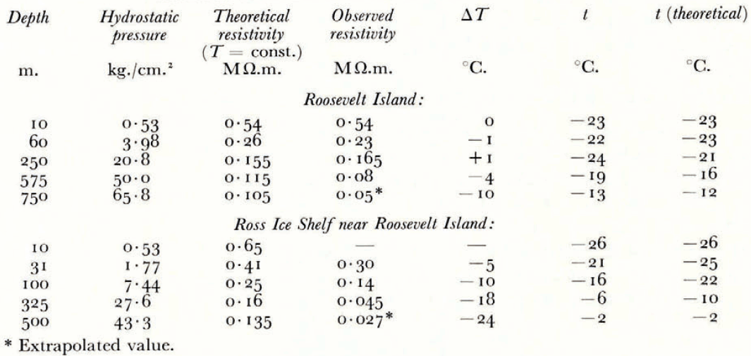
In Table II the depths of the central point of each layer are listed in the first column. The hydrostatic pressure at these depths (based on average densities from Antarctic pits and drill holes showing similar accumulation rates as Roosevelt Island) is given in the second column. The corresponding resistivities given by equation (3a) at surface temperature are shown in the third column. In the fourth column the calculated resistivities from the resistivity curves are listed. The difference between the two resistivities according to equation (1) gives the temperature difference ΔT. A simple method determining ΔT consists of drawing a straight line with the slope k/

on a plot of logarithm of resistivity against 1/T through the point (ρ ₁, T ₁). Theoretical temperatures for the centre of Roosevelt Island according to the theory of Reference RobinRobin (1955) and for the ice shelf near the island (no bottom melting) after Reference WexlerWexler (1960) are listed in the seventh column. At both locations these theoretical figures differ from the temperatures derived from electrical measurements. At Roosevelt Island, however, there is a fairly good agreement between the two temperatures if we allow a higher accumulation rate for the past (about 30 g./cm.² yr.; Fig. 5). On the ice shelf the temperatures from the electrical measurements agree poorly with theoretical values (Fig. 6). Higher accumulation rates or bottom melting would only enlarge the difference. The discrepancy may result from preferred crystal orientation brought about by high strain-rates.

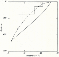
Fig. 5. Theoretical temperatures after Robin (solid curves with annual accumulation as parameter) and temperatures from electrical measurements (broken curve) for the ice cap of Roosevelt Island

Fig. 6. Theoretical temperatures after Wexler (solid curve) and temperatures from electrical measurements (broken curve) for the Ross Shelf Ice near Roosevelt Island

The apparent resistivity curve at “Station Centrale”, Greenland (Fig. 1) (lat. 70° 54.6′ N., long. 40° 38.0′ W., elevation 2,965 m., ice thickness 3,190 m., accumulation ≃ 30 g./cm.² yr., 10-m. temperature −28°C.) can be explained with the following four layer model:

The interpretation shows that down to 1,200 m. depth the variation of resistivity can be explained by a decrease of the contact resistance according to equation (3a) alone (except for the uppermost 100 m.) which means that the temperature of the Greenland Ice Sheet at “Station Centrale” down to 1,200 m. must be nearly constant. Nearly constant temperatures in the central region of ice sheets have been found in deep drill holes (Reference HeubergerHeuberger, 1954; Reference WexlerWexler, 1961) but no measurements deeper than 350 m. have been made. Approximately 1.2 km. may be the depth at which the temperature on “Station Centrale” starts to increase relatively rapidly. This figure would agree with theories of temperature distribution in ice sheets (Reference RobinRobin, 1955; Reference Jenssen and RadokJenssen and Radok, 1963) (Fig. 7).

Fig. 7. Theoretical temperatures after Robin (solid curve a) and Jenssen and Radok (solid curve b) and temperatures from electrical measurements (broken curve) for “Station Centrale”. Curve a was calculated assuming an accumulation of 30 g./cm.² yr.; curve b allows for frictional heat at the bottom of the ice sheet due to an average movement of 30m./yr.

At the moment the relative error of the temperature differences derived from electrical measurements is quite large (about 35 per cent). This error contains the uncertainty about the true resistivity at a certain depth and the experimental error of the constants in equations (1) and (3a). More detailed measurements in the future and also handling multi-layered models according to Flathe’s theorem with a computer will probably reduce the error.

Summary

Despite various reservations about the interpretation, this study shows that the resistivity on ice sheets is a function of the contact resistance between the grains and the temperature, if the effect of the structure of the snow and firn can be considered negligible. After eliminating the influence of hydrostatic pressure upon the contact resistance, we can explain resistivity variations by temperature variations which agree partly with theoretical temperatures.

A valuable contribution of the resistivity measurements on ice sheets seems to be the determination of the activation energy for the resistivity of cold sedimentary ice which was found to be much smaller

than the value so far known from laboratory measurements.

Acknowledgements

The author wishes to acknowledge the assistance of Prof. B. Brockamp and the members of the geophysical group of the E.G.I.G., and the help of Dr. C. R. Bentley, J. F. Clark, R. Heidemann and W. Unger of the Roosevelt Island parties 1961–62 and 1962–63 during the field work.