


Microartifacts, or “invisible” human-made artifacts, promise important insights into ancient human behaviors. Unlike their macroscopic (> 6.3 mm, or 0.25 in.) equivalents, people have difficulties removing them from activity areas. Their presence allows reconstructing the latter. For their analysis, archaeologists collect soil samples, sieve them into size fractions, and study each fraction under a microscope to count microartifacts. In the following, we focus on lithic microdebitage because it preserves better than other microartifacts (Sherwood Reference Sherwood, Goldberg, Holliday and Reid Ferring2001; Sherwood et al. Reference Sherwood, Simek and Polhemus1995) and because of extensive previous research (discussed below). In its traditional approach, lithic microdebitage analysis exemplifies archaeological “slow data.” According to Bickler (Reference Bickler2021:186), “Whereas ‘Big Data’ approaches focus on managing data flowing in on a continuous or near-continuous basis, archaeological data can be very slow to create—sometimes taking years or decades—and is delivered in large ‘lumps’ of complex contextualized information.” In the case of microdebitage analysis, scholars have to commit extensive time and labor. This has limited the number of samples and increased inter- as well as intraobserver errors. Although many archaeologists acknowledge the potential of microdebitage, they harbor doubts about its manual analysis. Here, we outline a new approach to microdebitage that combines experimental archaeology, dynamic image analysis, and machine learning. We define microdebitage as particles that result from lithic reduction and are smaller than 6.3 mm.
Archaeologists are starting to adopt machine learning, but their applications often suffer from small training datasets and inadequate statistical techniques (Bickler Reference Bickler2021; Yaworsky et al. Reference Yaworsky, Vernon, Spangler, Brewer and Codding2020). Recent studies tend to focus on large-scale phenomena such as mounds and agricultural terraces (Orengo et al. Reference Orengo, Conesa, Garcia-Molsosa, Lobo, Green, Madella and Petrie2020; VanValkenburgh and Dufton Reference VanValkenburgh and Andrew Dufton2020). The ARCADIA and ArchAIDE projects, as well as other researchers, have used convolutional neural networks to classify ceramic sherds (e.g., Anichini et al. Reference Anichini, Banterle, Buxeda i Garrigós, Callieri, Dershowitz, Dubbini and Diaz2020, Reference Anichini, Dershowitz, Dubbini, Gattiglia, Itkin and Wolf2021; Chetouani et al. Reference Chetouani, Treuillet, Exbrayat and Jesset2020; Pawlowicz and Downum Reference Pawlowicz and Downum2021; Teddy et al. Reference Teddy, Romain, Aladine, Sylvie, Matthieu, Lionel, Sebastien and Jennane2015). To our knowledge, we are the first to apply machine learning to microartifacts (see also Davis Reference Davis2021). We address critiques of traditional microdebitage analysis and make its data amendable to big data analysis.
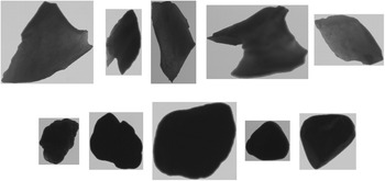
Here, we employ two sample datasets—experimentally produced lithic microdebitage and archaeological soil. To obtain a pure lithic microdebitage sample, we work with Michael McBride and other modern stone knappers who use traditional tools and raw materials (see below). We collect the debris and sieve out microdebitage. In addition to the experimental sample, we use a soil sample from the Classic Maya village of Nacimiento. A dynamic image particle analyzer allows us to describe each of the roughly 80,000 particles through dynamic image analysis (Figure 1; Eberl et al. Reference Eberl, Johnson and Aguila2022; Johnson et al. Reference Johnson, Eberl, McBride and Aguila2021). We then test how well machine learning algorithms differentiate between microdebitage and soil. Our models are based on Naïve Bayes, glmnet (generalized linear regression), random forest, and XGBoost (“Extreme Gradient Boost[ing]”) algorithms (for an overview of these algorithms, see Sammut and Webb Reference Sammut and Webb2017:208–209). The results suggest that random forest models are particularly well suited to identify lithic microdebitage.

FIGURE 1. Dynamic image particle analyzer photos of samples of chert microdebitage (top row) and soil particles (bottom row).
TRADITIONAL MICRODEBITAGE ANALYSIS
Stone knapping was essential in ancient societies before the widespread adoption of metal tools. Yet, many aspects remain obscure because knappers cleared products as well as debris from their workspaces (e.g., Clark Reference Clark1986a). Lithic microdebitage is too small, though, to be easily seen and collected (Fladmark Reference Fladmark1982). Its presence in soil samples helps archaeologists to reconstruct where and how knappers both produced and maintained stone tools (reviewed in Johnson et al. Reference Johnson, Eberl, McBride and Aguila2021:111–112).
More broadly, lithic microdebitage indicates buried archaeological sites and has helped with the evaluation of site-formation processes (Fladmark Reference Fladmark1982:215; Gé et al. Reference Gé, Courty, Matthews, Wattez, Goldberg, Nash and Petraglia1993:151; Nicholson Reference Nicholson1983; Sonnenburg et al. Reference Sonnenburg, Boyce and Reinhardt2011; for a critique, see Clark Reference Clark and Isaac1986b:23, 28–31). Contextual information is important. The floor composition influences the degree to which microdebitage remains. Gravel or earth floors (as in our case study from a Classic Maya village) offer many crevices for debris, whereas stucco floors are easy to keep clean (Spensley Reference Spensley, Laporte, Arroyo and Mejía2005:436). Natural postdepositional factors affect microartifacts (Hilton Reference Hilton2003; Mandel et al. Reference Mandel, Goldberg, Holliday and Gilbert2017:805). Burrowing insects and animals as well as plant roots can displace them; yet, Dempsey and Mendel (Reference Dempsey, Mandel and Gilbert2017:489) argue that spatial patterns remain discernible.
Scholars collect soil samples for microdebitage analysis. In the current approach, they use soil sieves in standardized sizes to separate the samples into size fractions (commonly from 0.125 mm [125 mu] to 6.3 mm [0.25 in.]—the size of sieving screens). Then they inspect each size fraction under a microscope and count the microdebitage particles. This approach requires extensive time, and it correspondingly has been applied to relatively small study populations. Published studies include up to 156 size fractions (discussed in Johnson et al. Reference Johnson, Eberl, McBride and Aguila2021:112). Traditional microdebitage analysis requires scholars to spend hours sorting soil samples under a microscope. This tedious work increases intra- and interobserver errors (Ullah Reference Ullah, Parker and Foster2012; Ullah et al. Reference Ullah, Duffy and Banning2015).
Many archaeologists are skeptical of manual, microscope-based microdebitage analysis. Scholars often assume that microdebitage is macrodebitage writ small—that is, each “invisible” flake is angular and transparent, and it shows some aspects of a conchoidal fracture or bulb of force (see also Fladmark Reference Fladmark1982:208–209). However, terms such as “angular” and “transparent” have not been defined objectively (see also Davis Reference Davis2020). In addition, the sheer number and small size of microdebitage particles has made it difficult to study whether proposed characteristics are consistently present across all size fractions. Scholars disagree on the threshold between macro- and microdebitage. Whereas some argue for 1 mm to stress the latter's invisibility, others set a 6.3 mm limit because archaeologists sieve out everything that falls through the common 0.25 in. screens (compare, in particular, Dunnell and Stein Reference Dunnell and Stein1989:34–35; Fladmark Reference Fladmark1982:205, 207). Here, we adopt the latter threshold but recognize the need to investigate this issue further.
A NEW APPROACH TO MICRODEBITAGE ANALYSIS
We are developing a new approach to microdebitage analysis that is based on experimental archaeology, dynamic image analysis, and machine learning. To quantify lithic microdebitage, we collect the debris of modern knappers, who employ traditional tools and raw materials to make stone tools. We then use a dynamic image particle analyzer to describe each microdebitage particle as well as particles from archaeological soil samples (Eberl et al. Reference Eberl, Johnson and Aguila2022). The output of this approach illustrates the challenge of microdebitage analysis. A handful of soil tends to contain hundreds of thousands if not millions of particles. Inspecting all of them manually is difficult in an objective and standardized way. We introduce machine learning to cope with the particle analyzer's big data (see also Bickler Reference Bickler2021).
For the current study, we use an experimental and an archaeological sample (Supplemental Tables 1 and 2). In 2019, stone knapper Michael McBride made a late-stage biface from a block of Edwards chert (Georgetown variety) from central Texas. He used deer antler and a deer antler–tipped Ishi stick for percussion and pressure flaking. We collected all debitage on a tarp and screened out the lithic microdebitage, or all particles smaller than 6.3 mm and larger than 125 mu. We assume that this chert sample—consisting of 5,299 particles—is representative of microdebitage. Eberl (Reference Eberl2014) collected the archaeological soil sample during his investigations at the Classic Maya village of Nacimiento in modern Guatemala. The sample came from a household midden. For this study, we took from this sample a few tablespoons of soil with a total of 73,313 particles. A visual inspection showed that it includes not only sand and gravel but also plant parts, ceramic sherd fragments, and other unidentified materials. Microdebitage studies sometimes prepare soil samples—for example, by soaking them in vinegar to remove organic materials (Fladmark Reference Fladmark1982:217–218); however, this step adds additional labor and time. To accelerate microdebitage analysis, we did not process our soil sample. Its complex composition means that the machine learning algorithms differentiate between lithic microdebitage and a heterogeneous other—an issue that we discuss further below.
We use a dynamic image particle analyzer to describe each particle (for more details, see Eberl et al. Reference Eberl, Johnson and Aguila2022). The PartAn3D measures dry particles ranging from 22 mu to 35 mm and comfortably covers microdebitage sample particles between 125 mu and 6.3 mm (particles at the extremes of the analyzer's range are less reliably measured). Samples are typically processed in a few minutes and require no sieving. Their particles fall from a vibrating chute and tumble by a high-speed camera. Software tracks each particle in multiple grayscale images and, given that the particle rotates while falling, measures it in three dimensions (Figure 1). The 39 variables include length, width, depth, angularity, and transparency (Eberl et al. Reference Eberl, Johnson and Aguila2022:318, Table 311). They are objectively defined (see below for angularity and transparency) and are given to three decimal places. For the roughly 80,000 particles of our two samples, Dynamic Image Analysis (DIA) takes or calculates approximately three million measurements. After tagging each particle of the two datasets as “site” or “exp(erimental),” we combined their measurements into one spreadsheet and applied machine learning algorithms to them.
MACHINE LEARNING METHODOLOGIES
Machine learning makes it easy to apply different algorithms to the same dataset (Bickler Reference Bickler2021:187). The resulting classifications can then be compared to select the best approach. For our study, we have applied four machine learning algorithms. In the following, we discuss Naïve Bayes, glmnet, random forest, and XGBoost.
Naïve Bayes algorithms assume that prior experience often serves best for selecting responses to unknown data. Bayes's theorem—expressed by the formula P(A|B) = P(A) × P(B|A) / P(B)—allows calculating the conditional probability of A (in our case, the classification of a particle into one of two classes) given true prior data B. The algorithm is called “naïve” because it assumes that all variables are independent—a rarely valid condition in real-world applications (Hastie et al. Reference Hastie, Tibshirani and Friedman2009:210–211).
Glmnet algorithms use generalized linear regression with elastic net, a regularized penalty. Similar to standard linear regression, these models use one or more predictor variables to explain a dependent variable (in our case, the particle class). It is “generalized” because it allows modeling of outcomes from a set of exponential distributions (e.g., binomial, Poisson, etc.) rather than being restricted to Gaussian distributions (i.e., standard linear regression; H2O.ai 2021). Regular linear regression tends to perform more poorly for datasets with more variables than samples or highly correlated variables. The “net” part in the glmnet algorithm adds regularization penalties to address this issue (Zou and Hastie Reference Zou and Hastie2005). During training, glmnet models penalize variables that contribute little and regularize them while also retaining groups of related variables.
The random forest algorithm creates multiple decision trees and, in the case of classification problems, selects the most common class as output (Breiman Reference Breiman2001). To improve on individual decision trees, this ensemble learner minimizes the correlation among the decision trees. It bootstraps aggregates or bags the training data by selecting random samples with replacements. Each tree also learns on a random subset of features. These measures result in unique training sets for each decision tree. They decrease the model's variance (and the likelihood of overfitting) while balancing its bias. Random forest models are generally more accurate than single learners, but their output tends to be less intuitive (“black box problem”).
XGBoost, or “Extreme Gradient Boosting,” is an advanced ensemble learner (Chen and Guestrin Reference Chen, Guestrin, Krishnapuram and Shah2016). It improves on the random forest approach by creating decision trees sequentially. Each step minimizes errors through gradient descent, and it boosts the influence of high-performing models. The “Extreme” moniker refers to parallelized processing, tree pruning, and lasso as well as Ridge regularization (for the latter, see the glmnet model).
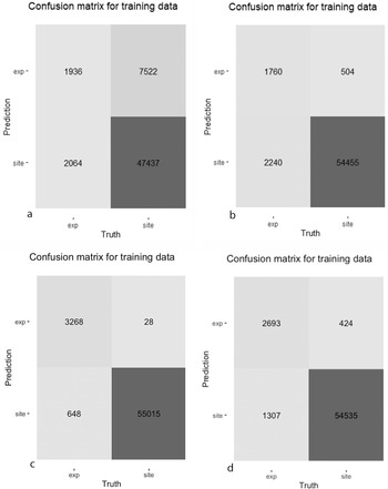
Machine learning often appears threatening because its results—in particular, many correlated variables—are difficult to understand for humans (Kissinger Reference Kissinger2018). Data scientists address some of these concerns through confusion matrices (Figure 4). For a binary problem such as ours, confusion matrices differentiate between two categories—microdebitage and other soil particles—and identify the number of correctly identified (true positives and negatives) as well as misclassified particles (false positives and negatives). Several performance metrics derive from the confusion matrix. The probability of detection (i.e., sensitivity/recall) measures the proportion of predicted true positives among all true positive particles. Specificity is the corresponding measure for negatives (it is of less importance here because our negative particles—archaeological soils—may, in fact, contain positives in the form of lithic microdebitage). The positive predictive value (PPV), or precision, expresses how many true positive particles were identified out of all particles predicted positive; the negative predictive value (NPV) is the corresponding measure for negatives. The F-score (more precisely, the F1-score) is the harmonic mean of precision and recall.Footnote 1 Accuracy measures how many particles were correctly identified. A roc curve plots the probability of detection (sensitivity) against the probability of false alarm (or false positive rate) for every threshold (during World War II, radar analysts developed the roc, or “receiver operating characteristic,” curve to describe the trade-off between better detecting enemy aircraft and generating more false alarms due to flocks of geese and other signal noise; Peterson et al. Reference Peterson, Birdsall and Fox1954). Machine learning algorithms maximize the area under the roc curve (roc auc). At last, precision and recall are plotted for every threshold; pr auc measures the area under the pr-curve. These metrics, or hyperparameters, can be used to provide insight into the performance of the model, and the ones most important to the application are used for model selection.
PROGRAMMING AND EVALUATING MACHINE LEARNING MODELS
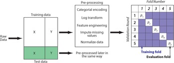
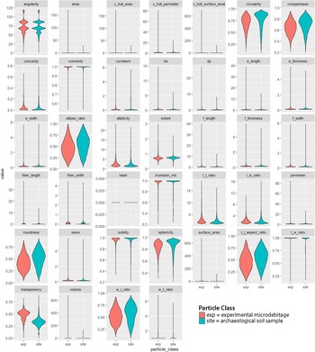
We programmed the four machine learning algorithms following standard data science procedures (Figure 2; Kuhn and Johnson Reference Kuhn and Johnson2019). The tuning of hyperparameters set them apart from common statistical techniques. For example, the glmnet algorithm is based on linear regression, but it introduces additional parameters that allow weighing the performance. The raw data were split into training (75%) and test data (25%). The latter are also known as a holdout set because they are kept apart until the end to judge model performance. After splitting, data were preprocessed to avoid data leakage. The visual inspection of variable distributions—for example with violin plots (Figure 3)—and statistical measures such as skewness help to identify potentially unusual values and relationships among variables. If necessary, missing values are imputed and data are log transformed or normalized.

FIGURE 2. Flow chart showing data split, pre-processing, and cross-validation.

FIGURE 3. Violin plots for 39 variables.
The training data was further divided into five random but equal-sized subsets or folds for k-fold cross-validation (Kuhn and Johnson Reference Kuhn and Johnson2019:47–55). Models were trained and validated multiple times and on different subsets of the data. In this way, the performance metrics of models become not too reliant on one specific dataset, and models should be able to perform better with new data. To optimize models, their hyperparameters were then tuned. The latter refer to parameters that users can vary. For example, in random forest models, hyperparameters include the number of decision trees and the maximum depth of the tree. Each machine learning problem is unique and correspondingly requires finding the optimal hyperparameters. Twenty model candidates cover a combination of different hyperparameters for each machine learning algorithm. The folds are used to determine the best performer by comparing hyperparameters. In addition, they allow us to evaluate whether splitting the data results in highly variable performance. High variance suggests that there is no overall trend in the data and that more data should be collected before generating a model. After training the four models, we identified the best-performing fold based on its metrics (Table 1). The hyperparameters were then used to fit the model on the training data (data scientists discourage selecting models based on their performance on the hold-out dataset because this would entangle the holdout with the training and selection process).
TABLE 1. Selected Performance Metrics of the Best Naïve Bayes, glmnet, Random Forest, and XGBoost Model.

Note: See Figure 5 for all model candidates.
Hyperparameters influence the behavior of models without being directly calculable; heuristics, sampling, and traversal of hyperparameter search spaces are often used to identify the values of hyperparameters suitable for a model. For glmnet, we explored the mixture (the relative weighting of l 1 vs l 2 regularization) and penalty (strength of regularization) hyperparameters. For XGBoost and random forest classifiers, we explored mtry (a parameter reflecting the number of predictors sampled at each split for creating the model) and min_n (a hyperparameter with a regularization effect that restricts nodes below a certain number of data points from being split further). We populate the hyperparameter combinations (grid) using a max entropy sampling, a space-filling design to enable adequate coverage of the total hyperparameter space given the constraints.
The metrics shown in Table 1 allow comparing the performance of any of these k-fold models for each algorithm. After picking one or two metrics that are relevant for our application, we select the hyperparameters that maximize that metric. The metric chosen to define the best model was the area under the precision-recall curve (pr auc). This is because the dataset is highly imbalanced. Usage of traditional area under the receiver operator curve (roc auc) reflects a relationship between the true positive and false positive rates, where the false positive rate is computed based on the total number of negative examples, which dominates the dataset. Consequently, pr auc provides a more sensitive metric for this application, particularly given our priorities of ensuring the identification of lithic microdebitage (sensitivity) and ensuring that predictions of the positive class are indeed correct (PPV). We then rebuild the model on the full training set (any model built during k-fold cross-validation is only built on a subset—n/k—of the training data). This forms the final model for a specific algorithm. We then compare these final models and select the best one based on our metric of interest.
RESULTS
Data exploration allowed us to visualize the differences between experimental microdebitage and archaeological soil particles (Figure 3). Violin plots for almost all variables have extremely long tails. Upon inspecting the raw data, we discovered repeated rows with nearly identical measurements that we excluded from further consideration.Footnote 2 In addition, the very thin and long tails of several violin plots suggest the presence of a few outliers. We left them in our data, but we discuss below whether they should be excluded. The two datasets—experimental microdebitage and archaeological soil particles—differ in several variables, most notably transparency and, to a lesser degree, circularity, sphericity, compactness, and others. These differences follow our expectations—namely, that lithic microdebitage is comparatively thin and less rounded than regular soil. They also suggest that the dynamic image particle analyzer data is suitable for differentiating between these two categories.
By comparing hyperparameters, we evaluated the performance of the four machine learning algorithms (Table 1). Random forest and XGBoost models performed best, followed by glmnet models and then Naïve Bayes models. We discuss individual performances and then evaluate their suitability for distinguishing lithic microdebitage.
The 20 Naïve Bayes model candidates varied widely in their performance (Figure 5a). The best performer—model candidate 14—reaches an accuracy of 83.7% and a precision of 20.5% (Table 1).Footnote 3 The relatively high accuracy of Naïve Bayes models is misleading because most of the data are soil particles, and a default classification as “soil” would be correct for most particles. The model identified only one out of five microdebitage particles correctly (Figure 4a). Among the variables, transparency, followed by compactness and roundness, and then the length–thickness ratio contributed most to the classification. The calibration curve indicates that this Naïve Bayes model is not well calibrated—that is, the scores generated by this model cannot be expected to correspond to true probabilities.

FIGURE 4. Confusion matrix for the best-performing models of four machine learning approaches (“exp” refers to experimentally produced microdebitage, and “site” refers to the archaeological soil sample): (a) Naïve Bayes, (b) Glmnet, (c) Random Forest, (d) XGBoost.
Unlike Naïve Bayes models, glmnet model candidates vary less in their performance (Figure 5b). Roc auc values between 0.87 and 0.91 indicate that the modeling performs well and is stable for all hyperparameters across the five folds. Very high specificity (~99%) indicates that the models almost always identify soil particles; on the other hand, sensitivity values around 40% reveal difficulties in identifying microdebitage (note that these observations are based on an untuned 0.5 threshold). Model candidate 17 turned out to be the best-performing glmnet model. Its sensitivity of 44.0% and a precision of 77.7% indicate that it identifies many microdebitage particles (Table 1). The confusion matrix shows that it classifies 1,760 microdebitage particles correctly and 504 incorrectly (Figure 4b). The variables that contributed most to the classification are length, convex hull perimeter, and the area equivalent diameter. Transparency is notably—and in contrast to the three other models—not very important.

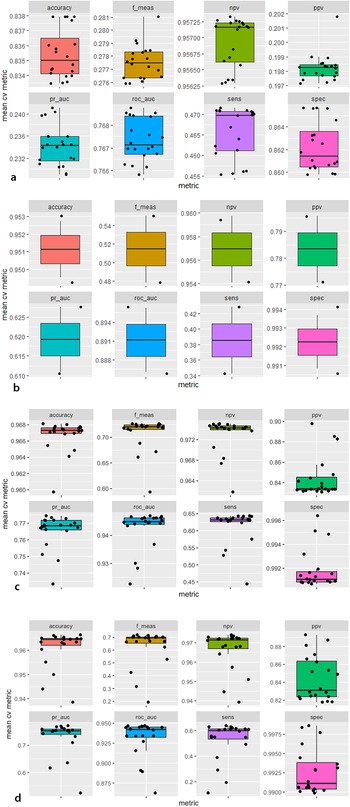
FIGURE 5. Distribution of mean cross-validation performance by 20 model candidates for each of the four machine learning algorithms (metrics are explained in Table 1; pr_auc refers to the area under the precision and recall curve, roc_auc to the area under the roc curve): (a) Naïve Bayes, (b) Glmnet, (c) Random forest, (d) XGBoost.
Random forest model candidates perform generally well, with tight areas under the precision-recall (median of about 0.77) as well as the roc curve (median of 0.95; Figure 5c). Their sensitivity of 63% and precision of circa 83% means that random forest models classify approximately two out of three microdebitage particles correctly, and that the ones they classify as microdebitage are in most cases correctly identified. Given the high area-under-the-curve scores, these values will likely improve with an optimized threshold. Model candidate 20, the best performer, differentiates cleanly between the microdebitage and soil. It misclassifies only 28 out of 3,296 microdebitage particles (Figure 4c). The 648 misclassified soil particles are probably microdebitage. Model candidate 20's sensitivity is 83.4%, and its precision 99.2% (Table 1). Transparency and (in a distinct second place) length are the variables that contribute most to the classification.
The XGBoost model candidates perform generally very well (Figure 5d). The area under the precision-recall curve is in the 70s, and the roc auc in the lower 90s. Model candidate 20 turned out to be the best performer. Its sensitivity (that is, the ability to identify microdebitage) is 67.3%, and its precision 86.4% (Table 1; these values are based on a not-yet-optimized threshold of 0.5). It misclassified 424 microdebitage and 1,307 soil particles. The latter are, as we note above for random forest models, less of a concern here because they likely reflect microdebitage in the archaeological soil sample. Transparency contributed by far the most to the model's performance, distinctly followed by solidity and Feret length.
DISCUSSION
Machine learning algorithms, experimental archaeology, and dynamic image analysis allow us to address issues with lithic microdebitage that have so far been unresolved. We discuss how to characterize microdebitage in standardized ways and how to deal with its variability. In addition, we debate our sampling strategy.
The lack of clearly defined characteristics hampers lithic microdebitage studies. Terms such as “angular” or “thin” are open to subjective interpretation. Dynamic Image Analysis (DIA) allows us to quantify the appearance of microdebitage by providing approximately 40 measurements for each particle. Fladmark (Reference Fladmark1982:208) characterizes microdebitage as highly angular but leaves what this means open. DIA defines angularity as the average angle change at each point of a particle's simplified outline (based on Wang et al. Reference Wang, Sun, Tutumluer and Druta2013). The resulting angularity index ranges from 0 (a perfect circle) to 180 (a particle with many sharp edges). Contrary to expectations, angularity does not contribute significantly to our machine learning models. The violin plot shows an overlapping distribution for the experimental and the archaeological sample. Angularity peaks four times, most pronouncedly at approximately 70 and 85. In the case of experimental microdebitage, smaller-size fractions lose the distinctive angular edges of larger flakes and appear round (for further discussion, see Eberl et al. Reference Eberl, Johnson and Aguila2022).
Objective definitions such as the one for angularity enable a quantitative characterization of particles. The large number of variables should not obscure, however, the fact that they do not measure the bulb of force. We argue that this is not a drawback. We have visually inspected our experimental microdebitage and observed comparatively few flakes—especially in smaller-size fractions—with a clear bulb of force. The current study indicates that various correlated and ranked variables can be used to characterize microdebitage. The differences among the four machine learning algorithms provide a basis to discuss relevant variable sets.
Transparency is critical for Naïve Bayes, random forest, and XGBoost models. This makes heuristic sense in view of the comparatively thin microdebitage particles (Fladmark [Reference Fladmark1982:208] lists transparency as a key characteristic of microdebitage). Dynamic image analysis allows us to quantify transparency. The particle analyzer takes multiple photos of each particle as it falls in front of a lighted back screen. The mean light intensity along the longest vertical line is recorded and averaged for all photos of the same particle. The value is then normalized to a 0–1 range, with 0 being least transparent and 1 being most transparent. The transparency of all particles in our archaeological soil sample averages 0.258 ± 0.172. This reflects the opaque sand kernels that make up most of it (see Figure 1). On the other hand, our experimental microdebitage sample is more transparent, with an average of 0.456 (± 0.163).
In addition to the question of which characteristics set microdebitage apart, it has remained unclear whether all microdebitage flakes share these characteristics. The violin plots that we have generated during data exploration (Figure 3) demonstrate the variability of lithic microdebitage. Above, we note their often very thin and long tails (Figure 3). These likely reflect a small number of outliers. Given that DIA tags and photographs each particle, we plan to filter them out and, if possible, identify them based on their appearance. It is possible that outliers reflect different types of particles.
This study focuses on the viability of different machine learning approaches. We used an archaeological soil sample to simulate a real-world application. This meant that we did not prepare the soil sample for this study to speed up its processing. We did not sort out ceramic sherd fragments, shells, roots, or any other artifact; we also did not remove smaller organic matter, for example, by soaking the soil sample in vinegar. The complex mix of particles impedes quantifying how lithic microdebitage differs from specific particles. For future studies, we propose four approaches. First, we will reanalyze archaeological soil samples under a microscope to identify microdebitage manually. This will allow us to evaluate the validity of the machine learning–derived results. Second, we plan to investigate the effect of different sample preparations on the performance of the machine learning models. Third, we will prepare experimental samples of known soil ingredients (e.g., sand and gravel) and compare them with the experimental lithic microdebitage. Fourth, we will study whether separating data into the traditional size fractions affects machine learning outcomes. The underlying issue is the need to understand whether microdebitage differs not only from regular debitage but also within size fractions.
CONCLUSION
Archaeologists recognize the potential of microdebitage analysis but remain skeptical about doing it manually. The traditional approach of sorting soil samples under a microscope not only requires time and effort but also introduces intra- and interobserver errors. Our approach to microdebitage analysis employs experimentally derived microdebitage, dynamic image analysis, and machine learning. The latter complements the first two components that we have discussed in other publications (Eberl et al. Reference Eberl, Johnson and Aguila2022; Johnson et al. Reference Johnson, Eberl, McBride and Aguila2021). These studies use multivariate statistics to differentiate microdebitage from other particles. The current study indicates that machine learning algorithms are similarly successful. Dynamic Image Analysis provides data on each particle in samples. By showing that even a small handful of soil tends to contain hundreds of thousands of particles, DIA demonstrates the challenge of microdebitage analysis. A human observer must look at all these particles under a microscope and sort out the knapping debitage. We argue that machine learning makes it possible to do this in an objective and standardized way.
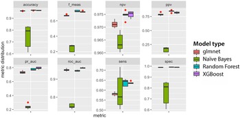
Above, we compare four machine learning algorithms—namely, Naïve Bayes, glmnet, random forest, and XGBoost (Figure 6). We conclude that the best random forest model offers the best performance, with a sensitivity of 83.5% and a 99.9% precision. It misclassified only 28 or 0.9% of lithic microdebitage. XGBoost models reach sensitivities in the upper 60s and precisions in the upper 80s. In other words, they identify two out of three microdebitage particles correctly, and the ones they identify are lithic microdebitage. On the other hand, the sensitivity of Naïve Bayes and glmnet models is below 50%—that is, less than half of the microdebitage is identified correctly. Naïve Bayes models also vary widely in performance, unlike models using the other algorithms. Our best XGBoost model underperforms our best random forest model. This is noteworthy because the XGBoost approach is often seen as superior to the random forest approach (Chen and Guestrin Reference Chen, Guestrin, Krishnapuram and Shah2016). Accuracy is often impressive (random forest models reach more than 99%), but it should be disregarded as a measure of performance for this study because the test data (N = 73,313) are more than a magnitude larger than the training data (N = 5,299), and identifying a particle by default as “soil” would be correct in most cases. Above, we also discuss ways in which we hope to improve the random forest and XGBoost models. In combination with dynamic image analysis, either model enables the objective study of lithic microdebitage and the processing of hundreds if not thousands of samples.

FIGURE 6. Comparing the performance of the four machine learning approaches. Red dots mark outliers (metrics are explained in Table 1; pr_auc refers to the area under the precision and recall curve, and roc_auc refers to the area under the roc curve).
Our study shows how machine learning can be applied successfully to an archaeological problem. Its data are comparatively small, and adding more is crucial to improve our models. Obtaining thousands or millions of data points is often challenging for archaeologists; we addressed this concern by switching to a dynamic image particle analyzer. The latter will allow us to add more reliable data quickly. Machine learning is not inherently superior; our four approaches differ starkly in their performance. Far from inscrutable black boxes, these approaches rely on well-known statistical techniques and their results—for example, the identification of transparency as key variable—are open to human inspection and reflection.
Acknowledgments
James Plunkett discussed with us the specifics of the PartAn3D particle analyzer. We thank Metin Eren as well as the anonymous reviewers for their thoughtful criticism. The senior author collected the archaeological sample under work permits of the Proyecto Arqueológico Aguateca Segunda Fase (directed by Takeshi Inomata, Daniel Triadan, Erick Ponciano, and Kazuo Aoyama) that Guatemala's Instituto Nacional de Arqueología e Historia issued.
Funding Statement
A Vanderbilt Strong Faculty Grant supported the purchase of the dynamic image particle analyzer.
Data Availability Statement
The software and data are available at https://github.com/vanderbilt-data-science/ancient-artifacts.git.
Competing Interests
The authors declare none.
Supplemental Material
For supplemental material accompanying this article, visit https://doi.org/10.1017/aap.2022.35.
Supplemental Table 1. Archaeological Soil Data Used for This Study.
Supplemental Table 2. Lithic Microdebitage Data Used for This Study.


 Open access