


INTRODUCTION
The importance of seasonal snow-cover to climatological, hydrological, ecological and anthropological processes over large areas in the terrestrial mid-to-polar latitudes of the Northern Hemisphere (NH) is difficult to overstate. Mankin and others (Reference Mankin, Viviroli, Singh, Hoekstra and Diffenbaugh2015) estimated that the runoff released by snowmelt provides the principal water resource through spring and/or summer for approximately two billion people across the NH, which hosts 98% of global seasonal snow-cover (Armstrong and Brodzik, Reference Armstrong and Brodzik2001). Snow also substantially transforms landscape physical characteristics, strongly influencing energy budgets through its high reflectivity and insulating effects (Zhang, Reference Zhang2005; Stieglitz and others, Reference Stieglitz, Déry, Romanovsky and Osterkamp2003). Because it occurs over relatively wide areas even at lower latitudes, it accounts for a greater fraction of cryospheric cooling in the NH than polar sea ice from January to April (Flanner and others, Reference Flanner, Shell, Barlage, Perovich and Tschudi2011). In ecosystems associated with climates where snow is the dominant phase of precipitation during the cooler months, many forms of biota have adapted specifically to the challenges and opportunities introduced by these conditions (Jones, Reference Jones1999).
Recognition of these key influences of seasonal snow, and of the potential for shifts from historical distribution patterns as a consequence of anthropogenic climate-change, has prompted a series of investigations into interannual trends in snow-covered area (SCA) and duration (SCD) (Groisman and others, Reference Groisman, Karl, Knight and Stenchikov1994; Clark and others, Reference Clark, Serreze and Robinson1999; Frei and others, Reference Frei, Robinson and Hughes1999; Brown, Reference Brown2000; Dye, Reference Dye2002; Rikiishi and others, Reference Rikiishi, Hashiya and Imai2004; Mote, Reference Mote2006; Déry and Brown, Reference Déry and Brown2007; Choi and others, Reference Choi, Robinson and Kang2010; Biancamaria and others, Reference Biancamaria, Cazenave, Mognard, Llovel and Frappart2011; Brown and Robinson, Reference Brown and Robinson2011; Cohen and others, Reference Cohen, Furtado, Barlow, Alexeev and Cherry2012; Liu and others, Reference Liu, Curry, Wang, Song and Horton2012; Vaughan and others, Reference Vaughan2013; Hernández-Henríquez and others, Reference Hernández-Henríquez, Déry and Derksen2015; Zhao and others, Reference Zhao2016; Yeo and others, Reference Yeo, Kim and Kim2017). Snowpack is inherently spatially heterogeneous (e.g. Pomeroy and others, Reference Pomeroy1998; Déry and others, Reference Déry, Crow, Stieglitz and Wood2004; Sturm and Benson, Reference Sturm and Benson2004) and terrestrial observation stations are distributed unevenly (Peng and others, Reference Peng2013), so remotely-sensed imagery has provided an invaluable resource from which to infer representations of SCA over large spatial domains. The datasets used, spatial and temporal frameworks adopted and metrics reported vary widely, so direct comparisons are seldom possible. However, these studies have consistently delivered four key messages.
Firstly, there is strong consensus that seasonal snow has been melting earlier in the NH spring, and that these losses have intensified during recent decades. Secondly, while overall SCA trends at continental scales are negative, some regions have seen augmented SCA in autumn and/or winter. Thirdly, snow-cover trends vary with latitude and elevation. Because snow persists longer in circumpolar and mountainous regions, and insolation potential increases through the spring and summer, it is to be expected that greater attrition would be identified in these contexts under warming atmospheric conditions. Indeed, enhanced climate-change signals have been detected in both the Arctic (Serreze and Barry, Reference Serreze and Barry2011) and mountain ranges (Fyfe and Flato, Reference Fyfe and Flato1999; Wang and others, Reference Wang, Fan and Wang2015; Sharma and Déry, Reference Sharma and Déry2016). However, no study has as yet described in detail the spatial distribution of trends in both SCA and SCD at regional scales across the NH throughout the year. Doing so would respond to the recommendation of Groisman and others (Reference Groisman, Karl, Knight and Stenchikov1994) that ‘centres of action’ of interannual SCA variability should continue to be monitored through time as key indicators of changing climatic conditions, and illustrate any seasonal variation of associations with latitudinal and elevational context. Generating a quantitative representation of these patterns was therefore identified as the principal objective of this investigation.
The fourth point of broad agreement is that NH SCA and SCD are strongly influenced by temperature and atmospheric circulation patterns. The accumulation and persistence of snow both depend on a range of influences: for example, sufficiently cold and humid air is required for snowfall to occur, whereas warm and/or dry and/or windy conditions accelerate its loss. It follows that cyclic patterns such as the El Niño Southern Oscillation (Groisman and others, Reference Groisman, Karl, Knight and Stenchikov1994); North Atlantic or Arctic Oscillation (Clark and others, Reference Clark, Serreze and Robinson1999; Biancamaria and others, Reference Biancamaria, Cazenave, Mognard, Llovel and Frappart2011; Brown and Robinson, Reference Brown and Robinson2011; Cohen and others, Reference Cohen, Foster, Barlow, Saito and Jones2010, Reference Cohen, Furtado, Barlow, Alexeev and Cherry2012; Liu and others, Reference Liu, Curry, Wang, Song and Horton2012; Zhao and others, Reference Zhao2016; Yeo and others, Reference Yeo, Kim and Kim2017); Atlantic Multidecadal Oscillation (Biancamaria and others, Reference Biancamaria, Cazenave, Mognard, Llovel and Frappart2011); Eurasian Type 1 Pattern (Clark and others, Reference Clark, Serreze and Robinson1999); Siberian Pattern (Clark and others, Reference Clark, Serreze and Robinson1999; Zhao and others, Reference Zhao2016); and the Pacific Decadal Oscillation, North Pacific Index and Pacific North American pattern (Mote, Reference Mote2006; Biancamaria and others, Reference Biancamaria, Cazenave, Mognard, Llovel and Frappart2011) play important roles in the distributions of SCA and length of SCD. Tracing the effects of these multiple meteorological drivers is complex, as they may vary monotonically as well as cyclically, and are further complicated by interference, resonance and teleconnection. A detailed consideration of these influences is therefore outside the scope of this study.
The primary aim of this paper is to build on earlier studies of snow-related trends at hemispheric and continental scales (Déry and Brown, Reference Déry and Brown2007; Hernández-Henríquez and others, Reference Hernández-Henríquez, Déry and Derksen2015) by generating a detailed description of spatial and temporal variations of snow-cover trends across the NH. As well as identifying contexts experiencing major shifts in snow climatology, this will help to identify areas in which changing patterns might signify increasing stress on summer water resources, provide a foundation on which to base analyses of attribution and contribute to the assessment of potential hydroclimatological regime transitions. The resultant description of intraannual variations in spatial distributions of snow-cover trends will also guide future validation studies of the dataset on which the analysis is based, thereby assisting with the quantification of associated uncertainties.
DATA
In common with prior related studies (Déry and Brown, Reference Déry and Brown2007; Hernández-Henríquez and others, Reference Hernández-Henríquez, Déry and Derksen2015), this analysis was based on the US National Oceanic and Atmospheric Administration's (NOAA) Climate Data Record of weekly visible NH snow-cover, compiled and curated by the Rutgers University Snow Laboratory (http://climate.rutgers.edu/snow-cover: Robinson and others, Reference Robinson, Dewey and Heim1993; Estilow, Reference Estilow2013 – hereafter the ‘NOAA – Rutgers Snow Dataset’, NRSD). With a Period of Record (PoR) dating from 1966, this dataset forms the longest satellite-derived record of any environmental variable (Estilow and others, Reference Estilow, Young and Robinson2015), and it has therefore been used repeatedly to study NH snow trends. It comprises a binary classification of snow-cover associated with snow-grid points (SGPs) at weekly intervals on a Cartesian 89 × 89 grid overlaid on the NH polar stereographic projection (Estilow, Reference Estilow2013). It is important to note that the area associated with each SGP (supplied with the dataset) varies with latitude, from ~10.7 × 10³ km2 at the lowest latitudes to ~41.8 × 10³ km2 near the geographic North Pole (Estilow, Reference Estilow2013).
Each temporal granule of the NRSD is generated over a 7-day period, from Tuesday to Monday. For a given week, if (on the latest day of that week on which it is unobscured by cloud on the source imagery) at least 50% of the area associated with an SGP is identified by the interpretative process as being snow-covered, the SGP is classified as such. This analysis used the same masks applied by the prior studies (Déry and Brown, Reference Déry and Brown2007; Hernández-Henríquez and others, Reference Hernández-Henríquez, Déry and Derksen2015) to exclude SGPs in oceanic areas or having a perennial cryospheric cover (mainly Greenland), together with an additional 33 SGPs previously associated with questionable snow-cover records (Déry and Brown, Reference Déry and Brown2007).
While the NRSD PoR begins in October 1966, it includes gaps during nine months between 1968 and 1971, so this study was based (as in Hernández-Henríquez and others, Reference Hernández-Henríquez, Déry and Derksen2015) on the continuous series from October (week 40) 1971 to September (week 39) 2014. The dataset was supplied directly by the Rutgers University Snow Laboratory in November 2014, and was identical to the ‘version 1 revision 1’ instance archived by NOAA to the same date (Robinson and others, Reference Robinson and Estilow2012; T. Estilow, personal communication, August 2017).
During its history, major advances in hardware and software capabilities have enabled a series of improvements to the sensors and processing algorithms used to generate the dataset: in particular, interpretation shifted from a primarily manual process to the more automated Interactive Multisensor Snow and Ice Mapping System in 1999 (Ramsay, Reference Ramsay1998). While considerable care has been taken to ensure overall consistency throughout the entire PoR (Romanov and others, Reference Romanov, Gutman and Csiszar2000; Helfrich and others, Reference Helfrich, McNamara, Ramsay, Baldwin and Kasheta2007; Estilow, Reference Estilow2013; Estilow and others, Reference Estilow, Young and Robinson2015), several authors have suggested that these developments may have resulted on the one hand in the identification of substantially more snow during the early stages of the annual snow-accumulation season (snow-onset), and less in the latter stages of the ablation season (snow-offset), giving rise to spurious positive and negative trends at these times, respectively (Wang and others, Reference Wang, Sharpa, Brown, Derksen and Rivard2005; Brown and others, Reference Brown, Derksen and Wang2007; Brown and Derksen, Reference Brown and Derksen2013; Hori and others, Reference Hori2017; Mudryk and others, Reference Mudryk, Kushner, Derksen and Thackeray2017). The PoR and spatio-temporal frameworks adopted by these studies contrast markedly with those described in this paper, so it is not possible to draw direct comparisons. However, it is hoped that new information generated by this analysis will help to guide further investigation of where, when and why the disagreements reported by these authors occur.
METHODS
Improved estimation of terrestrial area for coastal SGPs
The spatial extent associated with the NRSD SGPs was represented by Thiessen Polygons (TPs) (Fig. 1), generated using QGIS software (http://qgis.org). Marine areas within TPs were excluded using a regular grid of points at 10′ intervals, classified as terrestrial or oceanic by means of a QGIS spatial join with a spatial dataset of global land-masses. A second spatial join between the TPs and the 10′ points enabled computation of the terrestrial and oceanic fractions related to each SGP. Scaling the SGPs’ nominal areas by the former thus provided improved estimates of their associated terrestrial areas. The marine portions excluded amounted to 5.7% of the total area associated with the 1666 NRSD SGPs identified by the standard masks as being ‘terrestrial’ and having mean annual SCD of at least 1 week (3.1 × 10⁶ km2 of 53.8 × 10⁶ km2).

Fig. 1. NRSD snow-grid points (SGPs), with associated Thiessen Polygons (TPs) and corresponding areas. TPs coloured entirely grey or white are excluded from the analysis.
Estimation of ‘snow-dominated’ area
SCA is usually estimated from binary snow-cover classifications such as the NRSD by summing, for each temporal granule, the areas associated with spatial units classified as ‘snow-covered’. The implicit assumption is that ‘snow-covered’ (‘snow-free’) spatial units consistently have actual snow-cover of 100% (0%). However, ‘snow-covered’ cells in many spatio-temporal contexts often include snow-free areas, and vice versa: this leads to over- and under-estimation of SCA at different times of year, potentially exacerbated by specific land-cover types (Rittger and others, Reference Rittger, Painter and Dozier2013). This assumption would be expected to be particularly erroneous early and late in the snow-season, when actual fractional snow-cover may be slightly <50% in some years, and slightly more in others. However, this is the conventional approach on which prior studies have been based, and – in the absence of any reliable indication of actual fractional snow-cover throughout the full PoR – it is therefore also adopted here. A discussion of the possible implications of considering alternative assumptions is included in the section ‘Implications of considering alternative assumptions relating to the binary SDA classification’, but the key message is that the trends reported here relate more strictly not to changes in ‘snow-covered’ area, but in the area over which there is judged to be more snow-covered than snow-free terrain. Therefore, the term ‘snow-dominated’ area (SDA) is used hereafter.
Spatial aggregation and trend estimation
Bearing these points in mind, it is not meaningful to estimate areal trends for individual SGPs in a binary dataset. The investigation of spatial variations in SDA across the NH from the NRSD, therefore, required aggregation of SGPs within an appropriate spatial framework. This was achieved using a layer of cells drawn at regular 5° intervals of latitude and longitude, and identifying the SGPs falling within each (again using QGIS spatial joins). While this grid does not align with that adopted by the NRSD, the density of SGPs in the latter is sufficiently high compared with the partitioning imposed by the former (except at very high latitudes, where there is little or no terrestrial area) that adequate representation is achieved across the spatial domain. This partitioning scheme seeks a balance between competing considerations. On the one hand, it is fine enough to provide a useful representation of regional variations in trend signs and magnitudes, while reducing the effects of Scale and Zonation (or Aggregation) associated with the Modifiable Areal Unit Problem (e.g. Dark and Bram, Reference Dark and Bram2007). On the other, it is large enough that each spatial unit covers sufficient of the original SGPs that area-related trends could be estimated, while also being computationally and graphically manageable.
Total weekly SDA was computed throughout the PoR in each 5° cell as the sum of the terrestrial areas of all constituent snow-dominated gridpoints. The dataset includes details to support inference of the month(s) with which each weekly granule is associated, enabling monthly mean SDA values to be extracted. In this way, a time series comprising 43 SDA values (spanning 1971–2013 for October–December, 1972–2014 for January–September) was generated for each month in every 5° cell.
Because the surface footprint of the 5° cells decreases towards the North Pole, and also because individual cells include considerable oceanic fractions and/or SGPs excluded from the analysis by the various masks described previously, the terrestrial area of each cell represented within the NRSD varies considerably (further detail is provided in the Supplementary Material, Section S1). This constrains the maximum potential SDA in each cell, and therefore also its maximum possible trend magnitude when expressed in absolute units. In view of these considerations, SDA time series were also compiled for each cell as fractions of the total terrestrial area associated with the SGPs located within its footprint and included in the analysis (i.e. not excluded by the various masks). Trends generated from the absolute units are useful for providing metrics aggregated at regional to hemispheric scales, particularly for comparison with values from other studies, while those based on the fractional cover improve the spatial consistency of cartographic visualisation, and more directly support the quantification of associations with latitude and elevation.
Monotonic trends were identified from these series by Mann–Kendall Trend Analysis (MKTA: Mann, Reference Mann1945; Kendall, Reference Kendall1975), and the magnitudes of significant (p < 0.05) trends were estimated by least-squares regression. The rationale for using this approach, rather than the Theil–Sen method (Theil, Reference Theil1950; Sen, Reference Sen1968), is provided in the Supplementary Material (Section S2).
Snow-season duration
As described by Dye (Reference Dye2002), anomalies in the area and seasonal duration of snow-cover share a strong linear relationship. For consistency with the definition of SDA provided above, that used here for snow-dominated duration (SDD) is the count of weeks per snow-year (1 October–30 September in the following year) in which an SGP is flagged in the NRSD as being ‘snow-covered’ (i.e., its associated area is at least 50% snow-covered). The sub-set of NH SGPs with appreciable but clearly seasonal snow-cover was identified as those having median 1971–2014 SDD of at least 4 weeks and no more than 48 weeks. SDD trends were again identified by MKTA, and the magnitudes of significant (p < 0.05) trends quantified by least-squares regression. For this analysis, no distinction was made between the core and full snow seasons (c.f. Choi and others, Reference Choi, Robinson and Kang2010).
RESULTS AND DISCUSSION
Spatial distribution of SDD trends
Over the total area experiencing median seasonal SDD of 4–48 weeks (total area 47.3 × 10⁶ km2), significant (p < 0.05) negative SDD trends were identified for SGPs representing 23.3% (11.0 × 10⁶ km2), and positive trends were detected over 5.4% (2.5 × 10⁶ km2) of the same spatial domain. These trends are mapped in Figure 2, which also depicts associations between their spatial distribution and SDD climatology, latitude and topography (as derived from SGP nominal elevations provided with the dataset).
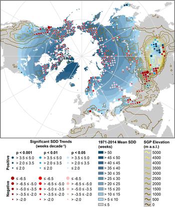
Fig. 2. Spatial distribution of significant (p < 0.05) trends in seasonal duration of SGP snow-dominance, overlaid on 1971–2014 mean annual SDD and coarse topographic contours derived from nominal SGP elevations.
Of particular note are the highly significant negative trends in south-central Eurasia (where the analysis suggests a reduction of SDD by as much as 23–32 weeks over the 43-year PoR), the Alborz and Zagros ranges of north-western Iran, the eastern front ranges of the Himalaya, the Rocky Mountains of western North America, and throughout the circumpolar regions of North America, Scandinavia and Russia.
In contrast, the only larger clusters of SGPs with significant positive SDD trends of appreciable magnitude are found in northern and eastern parts of the Himalayan region, including much of the Tibetan Plateau and in Japan and near the central Pacific coast of Russia. Other SGPs in which increases in SDD are implied are more spatially sporadic.
Remembering that the terrestrial area associated with SGPs varies (mainly with latitude), additional information is provided by scaling the magnitude of significant SDD trends (weeks (43 a)−1) by the corresponding SGPs’ areas, thereby expressing them in terms of the change in both time and area over which snow-cover is dominant through the PoR (km2 weeks (43 a)−1). Binning these metrics across the NH by SGP median annual SDD shows (Fig. 3) that positive trends occur mainly in areas where snow-cover of at least 50% usually persists for <~4–5 months of the year. This relatively short season is most likely to occur in the NH midwinter (~late November to mid-February), when day-length is short and maximum insolation potential low. This, in turn, attenuates the potential for disruption of energy budgets by a negative snow-albedo feedback during these times.

Fig. 3. Summed significant 1971–2014 changes in NH snow area-duration (km2 weeks), in bins of median SDD.
It will also be seen that negative shifts only marginally outweigh positive changes, so there is no major overall shift across the NH in areas with these relatively short snow-dominated seasons. In contrast, across areas where snow seasons of 28–44 weeks have historically been experienced (so that cover persists well into the spring and summer), negative trends dominate. With maximum insolation potential much higher during these times, particularly at higher latitudes, this will increase the absorption of solar radiation at the land surface, because terrestrial snow-free albedo is much lower than that when snow-covered. However, these effects would be expected to vary in strength with land-cover and topography.
The spatial associations apparent in Figure 2 suggest links between SDD trends and SGP elevation and latitude, so this was explored in more detail by linear regression (Fig. 4). The results indicate that the magnitudes of both positive and negative SDD trends strengthen with increasing elevation and at lower latitudes, but that the strongest sensitivity is between negative trend magnitudes and elevation. With both signs of trend thus stronger among the major mountain ranges at lower latitudes (Fig. 2), longitudinal variations were also explored. This revealed a clear split between the strongest negative (positive) trends on the highest westward (eastward) slopes of the south-Asian mountain ranges (Fig. 5). There also appears to be a preponderance of negative trends on the westward (i.e. windward) slopes of the North American Western Cordillera.

Fig. 4. Variation in significant (p < 0.05) 1971–2014 SDD trend magnitudes with (a) elevation and (b) latitude for SGPs with median (1971–2014) SDD of 4 to 48 weeks. All correlations are significant with p < 0.001.
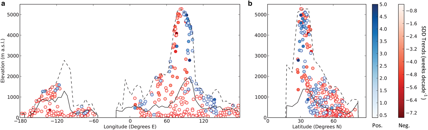
Fig. 5. Distributions of significant (p < 0.05) 1971–2014 SDD trends with elevation, (a) longitude and (b) latitude among SGPs with median (1971–2014) SDD of 4–48 weeks. The solid (dashed) lines represent meridional (in a) and zonal (in b) mean (maximum) elevations.
With the strongest trends of each sign thus identified at similar altitudes and latitudes, but with a clear longitudinal split relating closely to topography, it is difficult to account for them purely as artifacts of improvements in spatial resolution of the source imagery. A possible explanation for positive trends is that higher humidity in the warmer atmosphere, in conjunction with orographic uplift (and perhaps altered airflows), may have been augmenting snowfall in these contexts. Meanwhile, in upland areas across which losses are identified, exposure to circulations of warmer air in the free atmosphere may have been accelerating ablation, as suggested by Fyfe and Flato (Reference Fyfe and Flato1999). The longitudinal split between high-altitude SDD losses and gains identified here fits neatly with these invocations of contrasting atmospheric influences, particularly in the light of ideas relating to shifts in the frequencies and strengths of zonal and meridional airflows driven by amplified climate-change in the Arctic (e.g. Francis and Skific, Reference Francis and Skific2015).
While generally stronger at higher elevations (and thus lower latitudes), significant positive SDD trends are also identified for ~37 SGPs with associated nominal elevations below 2000 m and south of latitude 50° N. These are scattered along a latitudinal band ~ 40° N, from eastern through central Asia, southern Europe and near both coasts of North America. In general, these areas are associated with positive SDA trends during early winter, for which descriptions and possible causative factors are provided in the section ‘Spatio-temporal distribution of SDA trends’. However, some of these SGPs are close to the southern limit of the zone experiencing at least 4 weeks of snow-cover annually, and/or near coastlines: as snow extent will probably be less continuous in such contexts, it is possible that additional areas of this patchy cover have been identified by higher-resolution imagery deployed in the latter part of the PoR. These locales thus present an interesting focus for comparisons between the NRSD and ground observations or other remotely-sensed imagery.
The relative vulnerabilities of the snow-dominated seasons associated with SGPs experiencing significant negative SDD trends were quantified by dividing their 1971–2014 mean annual SDDs by the corresponding trend magnitudes (Fig. 6). While these values might in principle be interpreted as first-order approximations of the years remaining before the number of weeks with at least 50% snow-cover diminishes to zero, assuming a continued linear decline, it would clearly be highly simplistic to do so. Future reductions in SDD will depend heavily on rates of atmospheric warming (Kirtman and others, Reference Kirtman2013) and the amplification of SDA losses by the positive snow-albedo feedback (Thackeray and Fletcher, Reference Thackeray and Fletcher2016), so it is highly improbable that these trajectories will be linear.

Fig. 6. SGPs with significant (p < 0.05) negative SDD trends, rendered by quotients of 1971–2014 mean snow season length (weeks) and trend magnitude (weeks a−1). This (nominally) represents the number of years remaining, at current rates of change, until the annual count of snow-dominated weeks drops to zero. Shading (1971–2014 mean SDD) and contours (elevation m a.s.l.) as in Figure 2.
Nevertheless, this approach helps to identify focal points of dramatic shifts in snow climatology within the next few decades. By this measure, the areas likely to be most seriously affected are concentrated in the uplands south of the Caucasus into north-western Iran, from the Hindu Kush to the southern fringe of the Himalaya, and more sporadically in parts of southern Europe and western North America. It is notable that many of these SGPs are located within areas identified by Mankin and others (Reference Mankin, Viviroli, Singh, Hoekstra and Diffenbaugh2015) as depending on snowmelt to provide large fractions of otherwise unmet demand during the spring and summer months.
Spatio-temporal distribution of SDA trends
Overall, total NH SDA trends yielded from the NRSD vary in line with the annual solar cycle, with gains identified in autumn and winter and losses in spring and summer (Fig. 7). The majority of the significant trends identified are negative, and these dominate from March to September. Summed positive trends outweigh losses from October to February, but their total magnitudes and spatial extent are considerably smaller than the summer losses.

Fig. 7. Monthly variation in total NH SDA trend magnitudes (1971–2014) by statistical significance level.
The month of peak gains derived by these methods from the 1971–2014 PoR is December, in contrast to that identified from the NRSD using the spatial and temporal frameworks adopted by Mudryk and others (Reference Mudryk, Kushner, Derksen and Thackeray2017) and Hori and others (Reference Hori2017), which occurs in October. The maximum aggregate positive monthly trend identified by this analysis (0.415 × 10⁶ km2 decade−1) is ~40% of that reported in these studies. However, the timing and magnitude of peak losses in June broadly agree with their estimates. It is again important, though, to note that these estimated magnitudes are based on the erroneous – but, for practical purposes, currently unavoidable – conventional assumption that the areas associated with SGPs flagged as being ‘snow-covered’ (‘snow-free’) are 100% (0%) snow-covered: more realistic values would be considerably lower (see the section ‘Implications of considering alternative assumptions relating to the binary SDA classification’).
The maps in Figure 8 depict the 5° grid rendered by monthly SDA trend magnitudes (significant at p < 0.05) derived from time series of SDA as a percentage of cell terrestrial area. This provides a spatially consistent illustration of the variation in trend magnitude, by avoiding distortion within those 5° cells containing substantial oceanic areas and/or masked NRSD SGPs. (An equivalent map for trends expressed as absolute areas per unit time is available in Supplementary Material S3.) By comparing Figures 2 and 8, it will be seen that SDD trends coincide spatially with areas experiencing SDA trends, but that the latter vary in location, sign and magnitude through the year. They develop in the form of two extended pulses, one positive and the other negative: because the incidence of snow is controlled largely by latitude and elevation, the migration of these pulses is also guided by these attributes.

Fig. 8. Monthly distributions of NH SDA trends (1971–2014) as (% terrestrial area) decade−1 in (a) October–March and (b) April–September. (Shading represents topographic variation, from lower (darker) to higher (lighter) elevations.)
The positive pulse is moderate in strength, and more widespread and persistent on the Eurasian landmass than in North America. In contrast, negative trends are more widespread, of higher magnitude and identified at higher levels of statistical significance. Losses are seen initially at lower latitudes of central Eurasia in March and North America in April and May, before migrating rapidly northward, guided along pathways where the influences of latitude, elevation and continentality have in the past yielded extensive spring and summer SDA. With snow thus limited to the highest latitudes and altitudes by midsummer, negative trends largely dissipate and retreat, persisting through September only in the mountain ranges of western Canada and from the Himalaya to the Hindu Kush.
To complement this relative depiction, seasonal variations in trends derived from absolute SDA (km2 decade−1) in the 5° cells were aggregated within 20° (latitude) × 30° (longitude) patches (Fig. 9). These plots, together with representations of corresponding mean elevations, again show that both positive and negative trends may occur in a given month at comparable latitudes and elevations, but in different longitudinal ranges. For example, negative trends occur through most of the year on the western side of the Hindu Kush – Himalayan region, but positive trends are meanwhile seen in the eastern Himalaya and Tibetan Plateau. This corresponds with the identification of stronger negative SDD trends on the upper westward slopes of the south Asian ranges, and positive trends on the upper eastward slopes (Fig. 5). Indeed, more detailed figures relating SDA trend sign and magnitude to latitude, longitude and elevation (Supplementary Material Section S4) suggest that associations exist between positive trends and eastward slopes, and negative trends with westward slopes, in the mid-latitudes of both Asia and North America. The possibility thus arises again that interactions between atmospheric circulations, associated weather systems and (where appropriate) major topographic features are influencing these patterns, particularly in the light of recent studies relating changes in zonal/meridional airflows to shifting regional meteorological conditions (Screen and Simmonds, Reference Screen and Simmonds2010; Francis and Skific, Reference Francis and Skific2015; Wegmann and others, Reference Wegmann2015; Francis and others, Reference Francis, Vavrus and Cohen2017).

Fig. 9. Seasonal variations in significant (p < 0.05) 1971–2014 monthly SDA trends for 5° cells (as km2 decade−1) summed within 20° latitude by 30° longitude patches.
Associations between SDA trends, elevation and latitude
Figure 9 suggests that the NRSD records strong negative impacts on SDA climatologies, predominantly through the NH spring and summer in upland areas and in (the more generally lower-elevation) terrain at higher latitudes. However, the same plots suggest that positive trends coincide mainly with mountainous areas. Therefore, covariant associations were sought between monthly SDA trends of both signs and the latitudes and mean elevations of the 5° cells by linear regression.
The magnitudes of significant (p < 0.05) monthly SDA trends used here were again generated from the time series of SDA expressed as the fractional cover of terrestrial areas, to negate the influence of significant associations between latitude, elevation and the area of the 5° cells (Supplementary Material, Section S1). To simplify the visualisation of relationships between negative trend strengths and each influence, their absolute values were used. The elevation of each 5° cell was represented by the mean of the elevations of SGPs falling within it (as supplied with the NRSD), with its latitude taken at the cell centroid.
This analysis yielded significant correlations primarily in the NH summer (Fig. 10), with negative trends strengthening from April to August at higher latitudes, and in May and June at lower elevations. Significant correlations for positive trends are identified only in September, when they are found to strengthen at higher latitudes and lower elevations (noting again that a significant negative correlation exists between elevation and latitude, as detailed in Supplementary Material S1).

Fig. 10. Variation in correlation coefficients (Pearson's R) between monthly SDA trend magnitudes generated in 5° cells from % terrestrial snow-covered area (1971–2014) and (a) cell mean SGP elevation, (b) cell centroid latitude. Note that absolute values of negative trend magnitudes were used in the correlations, to simplify the representation of how their strengths relate to each potential influence.
Implications of considering alternative assumptions relating to the binary SDA classification
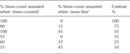
As described in the section ‘Estimation of snow-dominated area’, the estimates of trend magnitude presented here were derived using the conventional assumption that the actual area of snow-cover associated with an SGP flagged as being ‘snow-covered’ (‘snow-free’) is 100% (0%) of its associated terrestrial footprint. However, as demonstrated by Rittger and others (Reference Rittger, Painter and Dozier2013), this is seldom the case. Early and late in the snow-season, when the area covered by snow within each spatial unit passes through the 50% threshold, the contrast in actual fractional cover (AFC) between the two states may only be of the order of a few percentage points. In summer, while 0% AFC is generally much more feasible, 100% AFC is improbable even in the areas associated with highly snow-prone SGPs (remembering that this analysis seeks to exclude those with perennial cryospheric cover). Similarly, in winter (and given the NRSD's range of spatial resolutions) many ‘snow-free’ SGPs would reasonably be expected to have some appreciable amount of snow-cover. While the terminology employed here of ‘snow-dominated’ – rather than ‘snow-covered’ – duration and area aims to acknowledge and emphasise this point, it is useful to consider the results of making alternative assumptions about AFC in the two states. While these values would be expected to vary throughout the PoR for any given SGP and week, additional insights are provided by quantifying the effects of making different assumptions of the contrast between them as if they were fixed, and re-computing the trend magnitudes.
This was explored (using the same 1971–2014 PoR) for the months in which significant trends were identified within spatial units comparable with those adopted by Mudryk and others (Reference Mudryk, Kushner, Derksen and Thackeray2017), as follows: (a) pan-NH (‘NH’); (b) areas higher than 1500 m above mean sea-level (as indicated by the nominal elevation associated with SGPs within the NRSD: note that Mudryk and others (Reference Mudryk, Kushner, Derksen and Thackeray2017) distinguished their equivalent sub-unit as areas with standard deviation of elevation >200 m) (‘Alpine’); (c) lower-elevation areas poleward of latitude 60° N (‘Arctic’); and (d) lower-elevation areas south of latitude 60° N (‘Mid-Latitude’). In each scenario, a different percentage value was used to represent the AFC in the areas associated with ‘snow-covered’ and ‘snow-free’ SGPs (Table 1): the implicit monthly SCAs of each were then aggregated within these spatial units, and trends computed. (Additional detail of this process is provided in Section S5 of the Supplementary Material.)
Table 1. Scenario values of fractional snow-cover used to generate alternative time series of snow-covered area
The resultant magnitudes vary linearly with the contrast in AFC between the two snow-cover states (as listed in the ‘contrast’ column in Table 1), while the slope of this association varies with the month and sub-unit (Fig. 11). In every month, the Arctic sub-unit shows the highest sensitivity, driven by the larger surface area associated with SGPs at higher latitudes (Fig. 1). The sensitivity of the Alpine sub-unit is much lower, as most mountains are at lower latitudes, and the corresponding SGPs are therefore associated with smaller land-areas. It seems possible that Mid-Latitude sensitivities in July and August drop below those of the Alpine sub-unit because the only SGPs having any appreciable snow-cover in these months will be those associated with footprints including some mountains (though not over sufficiently large an area to raise the spatial mean elevation over 1500 m). These are again more likely to be found at lower latitudes, and are thus associated with smaller areas. Note that the sums of the sub-units’ sensitivities match those for the NH in May–August and December, but not in April or November, when only the Mid-Latitude and Alpine sub-units (respectively) exhibit significant snow-area trends. This implies that the pan-NH associations in these months (during which snow-cover would be expected to be transitional over large areas) may be exaggerated, as the overall snow-area trend depends on the aggregated areas within the sub-units for which significant trends are not individually identified.
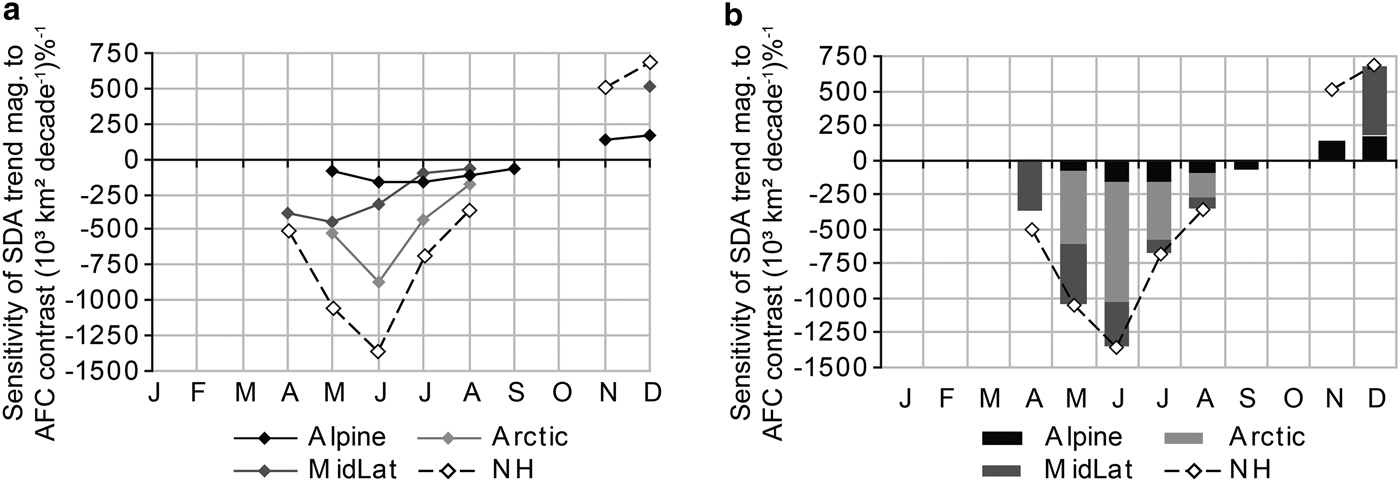
Fig. 11. Sensitivities of SDA trend magnitudes to the contrast in actual fractional cover assumed when spatial units are classified as ‘snow-covered’ and ‘snow-free’: (a) individually, (b) aggregated.
More generally, these findings present important implications for trend magnitudes computed from the NRSD. For example, the AFC in the area associated with a snow-prone SGP in a given week at the beginning and end of the snow-season would reasonably be expected to vary by a few percentage points either side of the 50% threshold from year to year. If the AFC during these times is of the order of 45% when flagged as ‘snow-free’ and 55% when ‘snow-covered’, this represents a contrast of only 10% between the two states, and the magnitude of a trend computed using this difference would, in turn, be only 10% of that generated using the conventional assumption of 100% contrast. Similarly, in summer (remembering again that this analysis sought to exclude areas with perennial cryospheric cover), the AFC in ‘snow-covered’ areas might be of the order of 55%, whereas that in ‘snow free’ areas would probably be close to zero, with a corresponding contrast of ~55%. The reverse actual coverages in snow-prone regions are more likely in winter, but the contrast would remain the same. In both cases, the resultant trend magnitudes would be around half of those estimated based on the conventional assumption. (Note that these percentages are purely speculative, to illustrate the effects of different contrasts between the two states.)
A further complication is that individual SGPs will be at different stages of their snow-season in a given week or month, depending on their physiographic and climatological characteristics. For example, SGPs with short SDD will generally experience later initial accumulation and earlier ablation of seasonal snow, so these transitions (in which lower AFC contrasts would be expected) will coincide with mid-season conditions (and contrasts) in areas with longer SDD. In this way, overall aggregated snow-area trends for a given month will emerge from a range of disparate AFC contrasts. It follows that trend magnitudes generated purely from the conventional assumption of 100% snow-cover contrast in AFCs between the two states should be considered as the outer bounds of an uncertainty range (i.e., maxima for positive trends, minima for negative trends), with the actual magnitude for a given SGP being considerably smaller during transitions to and from the snow-season than mid-way through its snowier and less-snowy seasons.
Information about the intraannual variation in the AFCs associated with SGPs, even if only as monthly climatologies, would thus help to reduce these uncertainties. In principle, it might be possible to estimate these through some – possibly most – of the NRSD PoR, for example by developing a form of data-assimilation or -fusion process, perhaps drawing on imagery from the successive Landsat platforms (which date from the early 1970s).
Notes on the credibility of the identified SDA trends
As noted previously, doubt has been cast by several authors on the credibility of the positive balance of SDA trends across the NH observed from October to December, and the strength of negative trends through the summer months (Wang and others, Reference Wang, Sharpa, Brown, Derksen and Rivard2005; Brown and others, Reference Brown, Derksen and Wang2007; Brown and Derksen, Reference Brown and Derksen2013; Hori and others, Reference Hori2017; Mudryk and others, Reference Mudryk, Kushner, Derksen and Thackeray2017). While this study adopts markedly different temporal and spatial frameworks, so direct comparisons are not possible, some observations on this topic are offered here. While some of the reported disagreements may have been driven by analytical assumptions or possible interpretive biases, it seems possible that others (particularly with modelled datasets) may relate to emergent climatological phenomena.
‘Snow-covered’ vs ‘snow-dominated’
The key point is that discussed previously, on the distinction between estimates of ‘snow-covered’ and ‘snow-dominated’ areas. When framed in the latter terms, the values reported here are more reasonable than if the former label is applied. Improved estimates of the magnitudes of trends in SCA, per se, will depend on identifying more representative ranges of the actual fractional area in spatial units when flagged in the two binary states, and of their intraannual variations. This will attenuate these estimates substantially, particularly early and late in the snow-season, but it would not change their signs. It is therefore also worth considering the possibility that the trends identified may, at least in part, be artifacts arising from extraneous influences.
Potential for bias in newly-deforested areas
Initial comparison with land-cover datasets suggests that many of the 5° cells in which positive SDA trends identified from the NRSD in October–December include large areas of coniferous forest. It is important to consider precisely what is meant by ‘snow-covered’ in such areas. Snow may lie on both the canopy and ground, or on the ground only. When classifying snow-cover, NRSD analysts seek to identify areas in which snow is expected to be on the ground, taking cues from visible patches in clearings – but this need not mean that it exists on the canopy (D. Robinson, personal communication, January 2016). Unfortunately, many published studies do not distinguish explicitly between these states, and this may confound comparisons.
Nevertheless, if spatio-temporal instances of positive SDA trends coincide with areas in which widespread deforestation has occurred during recent decades, and where natural (and intact) stand characteristics and climatology do not favour retention of canopy-intercepted snow – thereby providing few clues for the existence of snow on the ground – it is possible that the newly-cleared patches may have revealed previously masked areas of snow. Both logging and increased wildfire activity have resulted in clearances over large areas of Russia (Achard and others, Reference Achard, Mollicone, Stibig and Aksenov2006; Smirnov and others, Reference Smirnov, Kabanets, Milakovsky, Lepeshkin and Sychikov2013): meanwhile, widespread salvage logging in response to major pest infestations (e.g. Carroll and others, Reference Carroll, Taylor, Regniere, Safranyik and Shore2003; Bentz and others, Reference Bentz2010) and deforestation for hydrocarbon extraction (e.g. Pickell and others, Reference Pickell, Coops, Gergel, Andison and Marshall2016) continue in western North America. Such effects may have been further compounded by more of such clearings becoming apparent in the imagery of finer spatial resolutions. In principle, this might result in a progressive positive bias through the PoR. However, the possibility also exists that substantial areas of newly-unmasked snow may be driving a negative snow-albedo feedback, potentially contributing to wider and/or more persistent snow-cover. This presents an intriguing area for further investigation.
Ground observations and atmospheric circulations
Some support for positive trends is provided by observations of increasing snow depth, reported during the NH autumn and winter from ground stations across large areas stretching from eastern Europe to south-eastern Asia (Zhong and others, Reference Zhong2016). A mechanism has been suggested to link increasing early-season snow-cover in mid-latitudes, particularly in Eurasia, with the delivery of additional humidity from more ice-free Arctic waters by stronger meridional winds, driven by amplified waves in the Polar Jet (e.g. Cohen and others, Reference Cohen2014; Francis and others, Reference Francis, Vavrus and Cohen2017). It is therefore noteworthy that the results reported here identify a significant positive correlation between positive SDA trend-strength and latitude in September, when Arctic sea-ice area is at its annual minimum (Fig. 10). In an analysis of changes in the seasonal frequencies of high-amplitude waves, Francis and Skific (Reference Francis and Skific2015) found that such activity over Asia more than doubled during October–December between 1979–94 and 2000–13, the highest of any of the spatio-temporal units they considered by a considerable margin. This presents a particularly promising line of enquiry when seeking an explanation for the clear split between negative and positive SDA and (particularly) SDD trends on the highest westward and eastward slopes, respectively, of the major south-Asian mountain ranges (Fig. 5, and Supplementary Material S4). While several comparable studies have relied on the NRSD for snow-cover data, similar results have also been generated from observations recorded at an extensive network of Russian ground stations (Wegmann and others, Reference Wegmann2015).
One of the postulated drivers for these patterns is that widespread additional early-season Eurasian snow-cover has resulted in higher albedo and cooling of the lower boundary layer, thereby reinforcing the probability of such conditions persisting (Cohen and others, Reference Cohen, Furtado, Barlow, Alexeev and Cherry2012). The results presented here do not offer substantial support for this hypothesis, as significant SDA gains during October and November are identified over only a relatively small area of the eastern Asian mid-latitudes, implying additional snow-dominance of the order of 5% to 10% of terrestrial area per decade (over the 1971–2014 PoR). However, the area in which positive SDA trends are identified increases longitudinally and spreads further south during midwinter, moving in a broadly clockwise sweep around the eastern side of the area associated with the Siberian High. As maximum insolation potential at these lower latitudes is higher, perhaps a negative snow-albedo feedback is playing a role in such areas, depending in part on land-cover and topography. Associations between atmospheric circulation patterns, topography and additional atmospheric humidity thus offer a key avenue of continuing the investigation to improve understanding of early-season positive SDA trends.
Spring and summer trends in circumpolar lands
Another point of contention has been the strength of negative SDA trends during the summer months, particularly in circumpolar regions (Wang and others, Reference Wang, Sharpa, Brown, Derksen and Rivard2005; Brown and others, Reference Brown, Derksen and Wang2007; Mudryk and others, Reference Mudryk, Kushner, Derksen and Thackeray2017). As described in the section ‘Implications of considering alternative assumptions relating to the binary SDA classification’, the larger surface footprint associated with SGPs at high latitudes, in combination with the over-estimation of SDA trend magnitudes using the conventional assumption of a 100% contrast in the actual snow-covered fractional area associated with ‘snow-covered’ and ‘snow-free’ SGPs, is thought likely to account for much of the identified discrepancy. It would thus again be useful to obtain insights about fractional snow-cover climatologies, perhaps through some form of data-assimilation or -fusion process, potentially based on imagery from the Landsat or MODIS platforms.
However, inverting earlier discussion of the potential for land-cover influences on positive trends, there is also the possibility that increases in shrub vegetation over circumpolar lands may be obscuring patchy late-season snow (Mao and others, Reference Mao2016). On the other hand, as more prominent foliage develops, it is more likely to emerge through the depleting snowpack earlier in the season, thereby enhancing the snow-albedo feedback and hastening ablation (e.g. Ménard and others, Reference Ménard, Essery, Pomeroy, Marsh and Clark2014).
Potential influence of the modifiable areal unit problem
A final consideration is that the spatial framework adopted also limits the reliability of trend estimates. The pitfalls of using an arbitrary partitioning scheme to describe and explain geographical phenomena are well-established, and known in general as the Modifiable Areal Unit Problem (e.g. Dark and Bram, Reference Dark and Bram2007). Detailed consideration of this issue (and similar factors relating to the temporal framework used) is beyond the scope of this paper, but while the finer grid applied in this analysis helps to reduce the Scale Effect compared with those conducted at hemispheric or continental scales, the still-considerable size of each cell implies that they will often be heterogeneous in terms of their physiographic and climatological characteristics, so there are likely to be persisting problems relating to the Zonation (or Aggregation) Effect. Such influences may help to explain why some trends are spatially and/or temporally isolated, and this, in turn, could help to exclude artifacts. The authors are currently addressing this challenge in a related project, by adopting a more snow-aware segmentation at finer temporal scales. Nevertheless, the main positive and negative ‘centres of action’ presented here evolve with both spatial and temporal coherence, supporting the interpretation that they are driven primarily by interactions between climatological and physiographic influences, rather than being artifacts of improvements in sensor and/or processing technologies.
Potential implications for the water and energy cycles
This improved description of spatio-temporal distributions of long-term trends in seasonal cryospheric cover will help to identify key locales in which to investigate a range of linkages with the water and energy cycles. However, the scope for the assessment of potential impacts on the former is limited, without additional information describing associated variations in the depth and density of snowpack. New methods for inferring these details more accurately, particularly in complex or forested terrain – as sought by programmes such as NASA's SnowEx initiative (https://snow.nasa.gov/snowex) – are therefore essential. In conjunction with the spatial trends described here, they will inform assessments of shifts in the timing and intensity of freshet (melt-derived) flows, altered patterns of flood behaviour (Blöschl and others, Reference Blöschl2017) and/or reductions in streamflow and soil moisture (e.g. Berghuijs and others, Reference Berghuijs, Woods and Hrachowitz2014; Blankinship and others, Reference Blankinship, Meadows, Lucas and Hart2014). These, in turn, will help to quantify evolving pressures on water resources for human use, primarily where mountain ‘water towers’ have historically supplied large areas at lower latitudes through the warmer months (e.g. Barnett and others, Reference Barnett, Adam and Lettenmaier2005; Viviroli and others, Reference Viviroli, Dürr, Messerli, Meybeck and Weingartner2007; Immerzeel and others, Reference Immerzeel, van Beek and Bierkens2010; Callaghan and others, Reference Callaghan2012; Mankin and others, Reference Mankin, Viviroli, Singh, Hoekstra and Diffenbaugh2015). There are also indirect effects to consider: for example, positive SDA trends identified over the Tibetan Plateau may presage diminished summer rainfall in the south and south-east Asia (Wu and Qian, Reference Wu and Qian2003; Turner and Slingo, Reference Turner and Slingo2011); earlier inception of drier conditions could disrupt phenological cycles for vegetation (including crops) and migrations of anadromous fish species; and larger soil-moisture deficits in forests are thought likely to lead to more widespread wildfire activity (Westerling and others, Reference Westerling, Hidalgo, Cayan and Swetnam2006; O'Leary and others, Reference O'Leary, Bloom, Smith, Zemp and Medler2016).
Given that snow makes a greater contribution to atmospheric cooling than polar sea ice from January to April (Flanner and others, Reference Flanner, Shell, Barlage, Perovich and Tschudi2011), the development and expansion of negative SDA trends over large areas of central Asia in the spring months also have major implications. Their subsequent rapid expansion over sub-polar lands across Eurasia and North America through the summer adds to concerns over the likelihood of widespread thawing of permafrost, and consequent release of large volumes of ‘old carbon’, previously sequestered for thousands of years (Schuur and others, Reference Schuur2009). However, the quantification of impacts will rely on improved estimates of SCA and the rates at which they are changing, and of albedo variations in different landscape contexts.
CONCLUSIONS
The principal aim of this analysis was to describe spatial and temporal variations among significant trends in SDD and area throughout the NH, as represented within the NRSD from 1971 to 2014. It responds to the recommendation of Groisman and others (Reference Groisman, Karl, Knight and Stenchikov1994) that areas experiencing significant monotonic shifts in SDA should continue to be monitored closely within the context of a warming global climate. A purely graphical comparison reveals that the seasonal ‘centres of action’ of global variability in interannual snow climatology identified by this seminal study (which dates from well before the shift from mainly-manual to more automated interpretation using the Interactive Multisensor Snow and Ice Mapping System in 1999) largely coincide with the principal areas identified here as having experienced significant shifts in SDD and/or SDA.
It is again emphasised that these findings, being based on the conventional assumption of 100% (0%) snow-cover in ‘snow-covered’ (‘snow-free’) cells, represent the outer limits of uncertainty ranges for total SDA trend magnitudes: actual values, based on improved estimates of fractional snow-cover, are likely to be considerably smaller, particularly during the onset of the snow-season and the ablation period, and at higher latitudes in summer. It is worth noting, however, that the mountainous areas in which many trends are identified show relatively low sensitivity to this parameter.
Nevertheless, this analysis resolves the spatial distributions, signs and (maximum) magnitudes of monthly trends in SDA, describes their associations with elevation, latitude and longitude, and explores relationships with shifts in snow-season duration. As well as considering potential causative factors driven by climatological and physiographic influences, it presents possible alternative (or contributary) explanations for disagreements identified in prior studies between these metrics and other datasets, and suggests topics for future research aimed at reconciling these contrasting perceptions. These findings are therefore offered as a resource to guide and inform future hydrological, climatological, ecological and socio-economic studies relating to the changing seasonal cryosphere.
SUPPLEMENTARY MATERIAL
The supplementary material for this article can be found at https://doi.org/10.1017/aog.2017.47
ACKNOWLEDGEMENTS
This study was funded by the Climate Change and Atmospheric Research initiative of the Natural Sciences and Engineering Research Council of Canada, through the Canadian Sea Ice and Snow Evolution Network. We are grateful to Dr David Robinson and Mr Thomas Estilow of Rutgers University for making the NH snow-cover dataset available, and for providing helpful technical assistance. We also thank the Scientific Editor, Dr Charles Fierz and two anonymous reviewers for their constructive observations and recommendations, which helped to improve the manuscript.


 Open access