


Nomenclature
-
j = √-1
-
ϵ0 = 8.854185 x 10⁻¹² F m−1, the electric constant
-
ω = angular frequency (rad s−1)
-
f = frequency (Hz)
-
ϵ* = complex relative permittivity
-
ϵ’s = static relative permittivity
-
ϵ’∞ = high-frequency permittivity
-
Δϵ’ = ϵ’s– ϵ’∞ dispersion strength
-
ϵ” = dielectric loss factor
-
Tϵ = relaxation time (s) from permittivity data
-
Tσ = relaxation time (s) from conductivity data
-
σ* = complex conductivity (S m−1)
-
σ’s = static (or d.c) conductivity (S m−1)
-
σ’∞ = high-frequency conductivity (S m−1)
Introduction
The Antarctic Peninsula contains a wide variety of ice types reflecting the complete range of glacier facies and thermal regimes. Mean annual temperatures range from –25° (typically associated with dry-snow facies) to –3°C (associated with temperate glaciers).
The first direct current (d.c.) electrical experiments on ice in situ were carried out on temperate glaciers in Europe in the late 1950s (Reference RöthlisbergerRöthlisberger, 1967). Similar studies were conducted on cold polar ice in Greenland in the early 1960s, but the electrical properties found there were markedly different from those of European glacier ice which has a d.c. conductivity three orders of magnitude lower than that of polar ice (Reference Meyer and RöthlisbergerMeyer and Röthlisberger, 1962). Low-frequency alternating current (a.c.) experiments undertaken on ice cores in the laboratory (e.g. Reference Fitzgerald and ParenFitzgerald and Paren, 1975; Reference Glen and ParenGlen and Paren, 1975) have confirmed the extreme differences between temperate and polar glacier ice as found by in situ d.c. measurements. Ice grown slowly from pure water in the laboratory has similar d.c. conductivities to those of temperate ice (Reference Glen and ParenGlen and Paren, 1975). Polar ice samples that have been melted and refrozen in the laboratory have been found to behave like pure ice (Reference Fitzgerald and ParenFitzgerald and Paren, 1975; Reference Vassoille, Vassoille, Perez, Tatibouet, Duval and MaccagnanVassoille and others, 1982). The principal aim of the present study was to investigate in greater detail how natural ice samples that have been melted and refrozen in an ice shelf differ in electrical behaviour from firn and ice in a dry-snow facies and from ice from a temperate glacier. For this purpose, dielectric experiments were carried out at temperatures between –2° and –70°C in the frequency range 10 Hz to 100 kHz on 14 polycrystalline samples retrieved from six sites in the Antarctic Peninsula (Table I). Earlier studies in situ on George VI Ice Shelf have shown that the d.c. resistivity of ice formed from the percolation and refreezing of melt water is virtually indis-tinguishable from that of high-density polar ice formed by compaction of dry snow (Reference Reynolds and ParenReynolds and Paren, 1980, Reference Reynolds and Paren1984; Reference ReynoldsReynolds, 1982, unpublished).
Firn and ice cores were obtained by hand-coring to 10 m using an aluminium drill. The cores were maintained at temperatures around –20 °C for most of the journey to Cambridge, England, and throughout their storage. Sub-samples were taken from the cores and analysed (Table I). Each disc-shaped sub-sample was in turn placed in an electrode assembly in the form of a parallel-plate capacitor with guard rings. Its simple design has been described by Reference ReynoldsReynolds (unpublished). The electrode assembly was housed in an insulated enclosure in a variable-temperature environ-mental chamber. Measurements were made using a General Radio 1316 Oscillator, 1238 Detector, and a 1615 Capacitance Bridge. Values of the complex permittivity (ϵ*) and conductivity (σ*) of snow and ice were derived from measurements of capacitance and conductance. Whenever a temperature difference greater than 0.1 deg existed across the sample, capacitance and conductance components drifted which could have resulted in distorted dielectric dispersions. Dielectric measurements were obtained only after the bridge measurements at 1 kHz (general monitoring frequency) were repeatable to better than 0.1%. To achieve such repeatability after changing the chamber temperature, the enclosed samples had to be left for at least 18 h, thereby stabilizing both thermally and dielectrically. The parameters relate to a vertical electric field in situ, in common with all previous studies except those of Reference MaenoMaeno (e.g. 1978).
Table I. Details of Samples Retrieved From the Antarctic Peninsula

Dielectric Relaxation
The complex relative permittivity ϵ* of a dielectric, such as a monocrystal of pure ice, whose behaviour follows a Debye dispersion is given by:

The relaxation time T (which is temperature-dependent) is related to the relaxation frequency f R by the simple expression

At low frequencies the d.c. conductivity term predominates and produces a tail to the semi-circle on a Cole-Cole diagram. Equation (2) can be used to show that when σ’s > σ’∞/9 the influence of the d.c. conductivity extends to higher frequencies and no maximum (ϵ”max ) appears on the Cole-Cole diagram which is no longer semi-circular.
The complex conductivity σ* is defined by:
and the modified complex conductivity σ* m by:
An Argand diagram of σ’m against σ”m for different frequencies is known as an arc diagram and was first used by Reference GrantGrant (1958) and was applied to ice by Reference Camplin, Glen, Whalley, Whalley, Jones and GoldCamplin and Glen (1973), The arc diagram is a semi-circle for a dielectric whose behaviour is given by Equation (2). In a previous study of ice, the relaxation time of the conductivity arc diagram was assumed to be the same as that of its corresponding Cole-Cole diagram (Reference Camplin, Glen, Whalley, Whalley, Jones and GoldCamplin and Glen, 1973). This assumption is true in the case of an ideal Debye dispersion but is invalid in relation to natural snow and ice as will be demonstrated below.
Dielectric theory can be extended to describe a per-mittivity dispersion which has the form of a depressed arc:

where λπ/2 is the angle subtended by the ϵ’-axis and a line joining the low-frequency intercept on the ϵ ‘-axis with the geometrical centre of the dispersion.
An analytically more complicated permittivity dispersion is that in the form of a semi-ellipse. This results from a uniform distribution (on a logarithmic scale) of relaxation times between two limits, τh, and τl. According to Reference Camplin, Camplin, Glen and ParenParen and Glen (1978), if

where
Firn is a heterogeneous medium composed of air and of grains of ice. It is assumed that there are no dielectric or conducting processes associated with ice-air interfaces at grain boundaries and that the electrical properties of firn are determined by those of air and of solid ice. The per-mittivity of firn and bubbly ice is dependent on the ratio v of the density of the sample to that of solid ice whose permittivity is ϵ *i. A well-documented expression relating these parameters has been reported by Reference Glen and ParenGlen and Paren (1975) and is:
If ϵ*i follows a Debye dispersion, Equation (6) predicts a slightly distorted semi-circle for ϵ*f with essentially the same relaxation time when firn is being modelled. Using this relationship with ϵ’∞i = 3.2, the high-frequency solid-phase conductivity σ ∞ of firn is given by equation (10) of Reference Glen and ParenGlen and Paren (1975) where:
where subscripts f and i refer to firn and solid ice, respectively.
Results
For every temperature at which each sample was analysed Cole-Cole and arc diagrams were drawn from which values of ϵ’∞, ϵ’s, σ’∞, τϵ and τσ were deduced. Relaxation times were determined to within 1%. Permittivity maxima (ϵ”max) were not obtained for two ice samples (S1 and S3) at temperatures higher than –40° and –23°C. Firn sample (S2) had no maximum at –2° C.
Relaxation times (τσ) obtained from the maximum of ϵ* m arc diagrams were found to be up to four times smaller than those derived from the maxima of ϵ * diagrams (τϵ). Seventy-six values of the ratio of relaxation times τϵ /τσ obtained from 14 firn and ice samples are plotted in Figure 1 against an eccentricity parameter for the permittivity dispersions. The eccentricity parameter e is de-fined by:


Fig. 1. Eccentricity parameter e as a function of the ratio of relaxation times from complex conductivity (τ s ) and complex permittivity (τ ε ) dispersions. The dashed and solid lines have been derived from the theory of depressed arcs (Equation (4)) and of semi-elliptical dispersions (Equation (5)), respectively. The dots are experimental values.
The solid and dashed lines in Figure 1 have been derived from the theory of semi-elliptical dispersions (Equation (5)) and of depressed arcs (Equation (4)), respectively. Figure 1 shows that there is little to differentiate between the theoretically derived lines and experimental points for low eccentricities. Only when e exceeds 0.6 do the data fit the semi-ellipse theory better than that for the depressed arc. These results clearly demonstrate that permittivity and modified conductivity dis-persions have different frequencies at the maxima of their dispersions; the exception is the simple Debye dispersion where e = 0. To conform with convention, all subsequent discussions of relaxation time refer to the average time obtained from the Cole-Cole diagram (τϵ).
Typical Cole-Cole diagrams for two firn and ice samples are illustrated in Figure 2. As temperature decreases, so the dominant dispersion becomes more distinct and the low-frequency tail diminishes. Dielectric dispersions for ice samples are more eccentric than those of firn. The dispersion strength (Δϵ′) varies slightly with temperature. For ice, the maximum average dispersion strength (40) occurs at around –20 °C, decreasing to below 30 at –70 °C; for firn, the maximum average (16.5) occurs around –30°C. At the lowest temperatures investigated (–50° to —70°C) the average dispersion strengths for firn tend towards a constant (about 15).
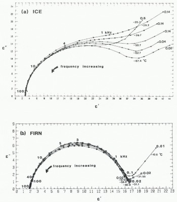
Fig. 2. Dielectric response of (a) sample S3 and (b) sample S8. Frequencies in kHz.
Figure 3 shows families of graphs of ϵ” against log frequency for one firn and one ice sample. Both families of curves exhibit similar features; a low-frequency tail which diminishes as temperature decreases, a clear ϵ “ maximum in the middle of the principal dispersion range, and lengthening relaxation times as temperature decreases. The relaxation times (τϵ ) have been plotted on an Arrhenius diagram as a function of 1/T where T is the temperature in degrees Kelvin (Fig. 4). Samples 2–4 and 6–8 cluster in the upper part of the diagram while samples 9–14 have dis-tinctly shorter relaxation times. The two groups of samples represent those from cold polar sites and those from warm temperate sites. Sample 5 lies between the two groups; its shape is more similar to that of the temperate samples. Why this one sample should appear to be transitional between polar and temperate samples is not known. Figure 4 also shows that samples from Deception Island have the shortest relaxation times and corresponds with the samples being naturally contaminated with volcanic material (ash and sul-phates) from the adjacent active vents. At high temperatures, the activation energy of each polar sample approached 0.56 eV, whereas below –20 °C the activation energy is found to be 0.21 ± 0.03 eV. The activation energies of the two temperate samples from Wormald Ice Piedmont (S9 and S10) and the four temperate samples from Deception Island (S10–14) are 0.20 ± 0.01 eV and 0.21 ± 0.03 eV, respectively. Thus, below –20 °C both polar and temperate ice samples have very similar activation energies.

Fig. 3. Dielectric loss factor (ϵ”) as a function of frequency and temperature for (a) sample S3 and (b) sample S8.
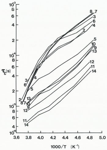
Fig. 4. Temperature dependence of relaxation times (t ε ) for 14 firn and ice samples from the Antarctic Peninsula.
In order to compare quantitatively the conductivity of firn with that of ice, the firn value has been adjusted to take account of its lower density by using Equation (7). Values of σ ∞i for nine samples have been plotted on an Arrhenius diagram (Fig. 5). Activation energies lie in the same range as found for the relaxation time. Three features need to be emphasized. First, the firn samples have a smaller range of conductivity at a given temperature than the ice samples. Secondly, the temperate samples have activation energies which increase as temperature decreases. In contrast, the activation energy of nearly all the other samples decreases as temperature decreases until about –50 °C. Thirdly, the temperate samples (S9 and S10) have noticeably higher solid-phase high-frequency conductivities than those for samples from colder sites.

Fig. 5. Solid-phase high-frequency conductivities (σ ∞i )of HCI-doped ice (from Reference Gross, Gross, Hayslip and HoyGross and others, 1980, nos. 1–4) and of HF-doped ice (from Reference Camplin, Camplin, Glen and ParenCamplin and others, 1978, nos. 5–9) compared with σ ∞i (heavy lines) of (a) four ice samples and (b) five firn samples from the Antarctic Peninsula. Approximate grain-size of each sample is given in brackets.
The high-frequency conductivity of a sample kept at a temperature higher than –10°C increased with time. AH Subsequent conductivities were noticeably higher by up to 40% for any temperature lower than the maximum temperature to which the sample had been subjected. In addition, the solid-phase high-frequency conductivity calculated using Equation (7) tends to increase with increasing averge grain-size which is listed in Table I (Fig. 5).
Discussion
High-frequency conductivity
High-frequency conductivities of ice at –45°C (σ’∞45) from a wide variety of sources have been compared with those of the samples from the Antarctic Peninsula (summarized in Table II). The activation energies of firn and ice samples from the Antarctic Peninsula (0.21 ± 0.02 eV) are similar to the values for deep polar ice of around 0.24 ± 0.03 eV (Reference Glen and ParenGlen and Paren, 1975). Absolute values of σ’∞45, for ice-shelf and plateau samples are about half those of deep polar ice. The values of σ’∞45 for temperate polycrystalline samples are approximately 50% higher than those for deep polar ice and nearly 20 times greater than that of temperate monocrystalline glacier ice. The activation energies of the polycrystalline samples are less than half of the value given by Reference Glen and ParenGlen and Paren (1975) for the monocrystalline sample.
The formation of ice samples in the laboratory by melting and subsequently refreezing portions of polar ice cores is comparable to that of ice layers within firn in the percolation/soaked zone of sub-polar glaciers such as at the surface of George VI Ice Shelf. Two studies of the effects of such melting and refreezing of polar ice are given as examples of work undertaken previously. Reference Fitzgerald and ParenFitzgerald and Paren (1975) examined two samples from the “Byrd” ice core and Reference MaccagnanMaccagnan (unpublished) samples from Dome C. Both studies found that the dielectric behaviour of the modified ice was similar to that of ice monocrystals, i.e. the behaviour of the samples had radically altered by the melting and refreezing. For example, the activation energy for σ’∞i of the “Byrd” ice-core samples before modification was 0.24 ± 0.03 eV (Reference Fitzgerald and ParenFitzgerald and Paren, 1975). After refreezing, the activation energy for one sample altered to 0.5 eV above –20°C, and to 0.37 eV in the temperature range –20° to –60 °C. The activation energy of the other sample changed from 0.5 eV above –35 °C to 0.09 eV between –35° and -50°C (Reference Fitzgerald and ParenFitzgerald and Paren, 1975). In marked contrast, activation energies of 0.56 eV (temperatures greater than –20 °C) and of 0.21 ± 0.02 eV at temperatures below –20 °C were observed for the samples from George VI Ice Shelf. Reference Boned, Barbier, Whalley, Whalley, Jones and GoldBoned and Barbier (1973) found that the activation energy of the Debye dispersion in laboratory-grown polycrystalline ice decreases with time. The refrozen samples of Fitzgerald and Paren, and of Maccagan, were examined within days of being formed, whereas the ice layers within the firn of George VI Ice Shelf are several years old. Alternatively, the samples from George VI Ice Shelf have not undergone complete melting before re-freezing.
High-frequency conductivities (σ∞i ) of nine samples from the Antarctic Peninsula have been compared in Figure 5 with values of σ∞i for doped ice samples studied by Reference Camplin, Camplin, Glen and ParenCamplin and others (1978), and by Reference Gross, Gross, Hayslip and HoyGross and others (1980). The Antarctic Peninsula data match the trends of the published σ∞i values for HF- and HCI-doped ice remarkably well. The conductivities of all the Antarctic Peninsula samples, from coastal to remote inland sites, lie in the range of those of laboratory ice doped with concentrations of HCI between 0.4 and 255 ng g-1. These concentrations embrace those measured for present-day firn on the plateau of the Antarctic Peninsula (60 ng g-1) and the higher values expected at coastal sites (100-200 ng g−1) (Reference Mumford and PeelMumford and Peel, 1982), A consistent feature of Figure 5 is that the conductivity behaviour of the samples from the coastal sites reproduces that of the more highly doped laboratory samples. Reference Mumford and PeelMumford and Peel (1982) have shown that the predominant impurities in the snow of the Antarctic Penin-sula are marine ions such as Na, CI, and Mg which are found in similar ratios to those found in sea-water and thus marine aerosols are incorpated stoichiometrically into the firn. In laboratory-grown samples, impurities such as NaCl are not incorporated stoichiometrically; CI− is taken up preferentially to Na+, creating an acidic ice. NaCl concen-trations in polar firn should have less effect on electrical conductivity than an equivalent CI− concentration in an acidic ice grown in the laboratory from NaCl and HCl solutions. The comparison between laboratory-grown samples with a single dopant and natural ice with a range of im-purities is important in one respect; the high-frequency data for natural firn and ice can be recreated by laboratory-grown ice containing a single dopant.
Table II. High-Frequency Conductivity of Ice at –45 °C (Based on Reference Glen and ParenGlen and Paren (1975, Table I))

Solid-phase high-frequency conductivities of a sample from each of the three contrasting sites in the Antarctic Peninsula are compared in Figure 6 with those previously published for a variety of polar and artificial ice types. Of the samples from the Antarctic Peninsula, those from temperate sites have the highest σ’∞ as well as having the lowest d.c. conductivity, σ’ s, as found by in situ studies (Reference Reynolds and ParenReynolds and Paren, 1984). The behaviour of all samples from the Antarctic Peninsula converges close to 0 °C.
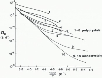
Fig. 6. Temperature dependence of the high-frequency conductivity σ∞(at 100 kHz unless slated otherwise):
-
1. Little America (personal communication from W.B. Westphal), 300 MHz.
-
2. Wormald Ice Piedmont, Antarctic Peninsula (this paper).
-
3. Ward Hunt Ice Shelf (personal communication from W.B. Westphal), 300 MHz; Camp Century and Site 2, Greenland (Paren, 1973); Byrd Station. Antarctica (Reference Fitzgerald and ParenFitzgerald and Paren, 1975).
-
4. George VI Ice Shelf (this paper).
-
5. Palmer Land plateau (this paper).
-
6. Polycrystalline “commercial” ice (Paren, unpublished).
-
7. Ice from TUTO tunnel, Greenland (Paren, unpublished).
-
8. Polycrystalline ice of figure 11 of Reference Camp, Camp, Kiszemck, Arnold, Riehl, Riehl, Bullemer and EngelhardtCamp and others (1969), 20 kHz.
-
9. Monocrystal, Ruepp (in Reference Glen and ParenGlen and Paren, 1975), 300 kHz.
-
10. Mendenhall Glacier monocrystal (Reference Glen and ParenGlen and Paren, 1975); monocrystal K70 of Reference Ruepp, Whalley, Whalley, Jones and GoldRuepp (1973), 300 kHz. (Figure based on Reference Glen and ParenGlen and Paren (1975, fig. 3).)
Values of the high-frequency conductivity at –45 °C of the ice component (σ ∞45 ) of firn and ice samples from the Antarctic Peninsula are compared in Figure 7 with those from samples from other polar glaciers. If polar ice is uniform in its behaviour and the correct conversion has been made between σ’∞f and σ’∞i, then σ’∞i should be independent of density and sample origin. Figure 7 shows that the Antarctic Peninsula samples indicate some independence of density but not of thermal regime. Samples from temperate sites (9–14) have a common conductivity around 8 x 10⁻⁶ S m−1 at –45°C. Conductivity values of polar samples (1−8) are scattered in the range (4 ± 2) x 10−6 S m−1 with five of the samples having a common value close to 2.5 x 10⁻⁶ S m−1. This is half the self-consistent value found for deep ice at Byrd Station, Camp Century, and Ward Hunt Ice Shelf. Figure 7 also shows that the conductivity values of the low-density Antarctic Peninsula samples are smaller than those of samples from the Mizuho cores studied by Reference Maeno and KuroiwaMaeno (1974) which show evidently a strong density dependence. For the finely divided ice of Reference Paren and GlenParen and Glen (1978) annealing raised the conductivity as indicated by the sequence of values shown in Figure 7 (personal communication from J.G. Paren). All the σ’ ∞ values of non-annealed samples are around (6 ± 4) x 10−6 S m−1 with little or no discernible trend with ice-volume fraction.
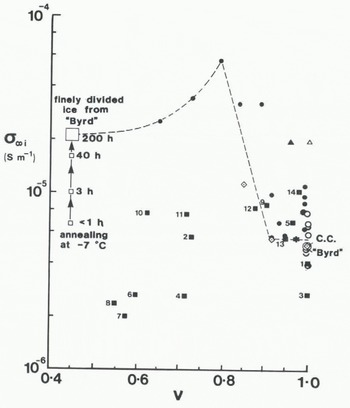
Fig. 7. Ice-volume fraction (v) dependence of the solid-phase high-frequency conductivity (σ∞1) at —45°C for samples described in the sources listed in Table III.
Direct-current conductivity (σ′ s )
The σ′s values obtained from dielectric measurements are up to three orders of magnitude smaller than the d.c. conductivities derived from four-electrode resistivity sounding in situ (Reference ReynoldsReynolds, 1982; Reference Reynolds and ParenReynolds and Paren, 1984). Similarly low d.c. conductivities have been reported for shallow cores from Mizuho, Antarctica (Reference MaenoMaeno, 1978), and Greenland (Reference KoppKopp, 1962). In common with Reference MaenoMaeno (1978), difficulties in fixing the specimens to the electrodes are suspected to have resulted in a less-than-ideal ohmic contact. Metallic electrodes cannot interface properly with ice. In a dielectric experiment, point defects accumulate at the ice/electrode interfaces which has the effect of reducing the d.c. conduction (Reference Petrenko, Petrenko, Whitworth and GlenPetrenko and others, 1983). Alternatively, some of the retrieved samples used in laboratory experiments may have aged thermally after being drilled from the ice sheet and transported to the laboratory. Samples from Camp Century, Greenland, and Byrd Station, Antarctica, used by Reference Paren, Whalley, Whalley, Jones and GoldParen (1973), and Reference Fitzgerald and Paren Fitzgerald and Paren (1975) do not seem to have been adversely affected. However, the first two reasons are thought to be the most probable ones.
Table III. Sources of Data and Key for Figure 7

Dielectric dispersion
The average dispersion strength (Δϵ 1) for the Debye dispersion for polar firn samples from the Antarctic Peninsula is 15.5 for a mean density of 0.58 Mg m-3 This compares well with 15.1 for firn samples studied by Reference Paren and GlenParen and Glen (1978) and Reference KoppKopp (1962). Both of these values are significantly smaller than the average Δϵ 1 of around 40 for shallow firn of comparable density from the Mizuho plateau (Reference Maeno and KuroiwaMaeno, 1974). The average Aϵ1 for Antarctic Peninsula ice samples is 44, which is almost half the value for laboratory-grown pure-ice samples (Reference Auty and ColeAuty and Cole, 1952) but in the same range as found in HF-, HCI-, and NH3-doped ices (Reference Camplin, Camplin, Glen and ParenCamplin and others, 1978; Reference Gross, Gross, Hayslip and HoyGross and others, 1978, Reference Gross, Gross, Hayslip and Hoy1980; Reference HubmannHubmann, 1978). Ice sample S9 has a dispersion strength of only 24. The dispersion strengths of snow and ice samples (with an upper density of 0.84 Mg m−3) are all less than 25 at –45°C except for Maeno’s samples from Mizuho plateau. At higher densities the dispersion strengths increase greatly to an average of 84. Although Maeno’s dispersion strengths are much higher than others, he too noted a change in behaviour at around 0.83 Mg m−3, the density at which the air passages between grains close off (Reference PatersonPaterson, [c1981], p.6).
Relaxation time
Relaxation times from Figure 4 are compared in Figure 8 with previously published data from other high-latitude sites and with values for pure ice, at –45°C. The data comprise two distinct sets. The set with longer relaxation times is tightly grouped and is associated with samples from sites where the mean annual temperature is lower than –10°C. The remaining samples are distinctly different. They all originate from with 7 km of the coastline of Antarctica a where the ice is temperate (i.e. at O°C throughout) but with two exceptions, Mizuho and Terre Adélie (D10. 46 m.B.). It can be seen from Figure 8 that the samples from Camp Century, Greenland, and Dome C, and Terre Adélie (D10. 46 m.H), Antarctica, possess remarkably similar relaxation times to those of samples from cold sites in the Antarctic Peninsula. The relaxation times of polar samples are about ten times longer than those measured for Japanese snowfall (line B, Fig. 8) of density 0.38 Mg m−3 (Reference Fujino and ŌuraFujino, 1967) and for annealed synthetic snow samples (line A, Fig. 8) made from pure monocrystals and from polar ice cores (Reference Paren and GlenParen and Glen, 1978). The data from Mizuho and Terre Adélie (D10. 46 m.B.) appear discordant as both have low mean annual temperatures (–33 ° and –13°C, respectively) and thus would be expected to behave like polar samples. Both sets of seemingly anomalous data can, however, be explained. It has already been stated that annealing of ice produces significant irreversible changes in its dielectric behaviour. The Mizuho samples studied by Maeno were obtained using a thermal drill (Suzuki and Takizawa, 1978). Consequently, the retrieved samples may have enhanced conductivities and shorter relaxation times because of the warming caused by the hot drill tip and the associated melt water. This could also explain why Maeno’s σ∞i data in Figure 7 are significantly higher than those of any other worker. In the case of the sample from Terre Adélie, D10. 46 m.B has a very low static electrical conductivity comparable to that of samples from the temperate Glacier d’Argentière and isotopically is a summer (i.e. warmed) layer (Reference MaccagnanMaccagnan, unpublished, p. 62). If these explanations are physically realistic, it demonstrates that the dielectric behaviour of natural polycrystalline ice is strongly indicative of its thermal regime. The corollary of this though is that some of the samples from George VI Ice Shelf, which have been interpreted previously as having melted and refrozen, should exhibit temperate-type dielectric behaviour. Figure 8 demonstrates that all of them, bar one (S5), exhibit polar charcteristics. This is either enigmatic or the samples in question have not undergone complete melting and refreezing as formerly thought; the latter is the more probable.

Fig. 8. Temperature dependence of relaxation times (Tε) for firn and ice samples from the Antarctic Peninsula. Polar-type behaviour is indicated by shading with crosses; temperate-type behaviour by shading with dashes. Also shown are data from : A: synthetic snow (Reference Paren and GlenParen and Glen, 1978); B: Japnese snowfall (Reference Fujino and ŌuraFujino, 1967): C: pure ice (Reference FitzgeraldFitzgerald, unpublished). The hatched area represents data from Mizuho plateau (mean annual temperature –33°C) (Reference MaenoMaeno, 1978). Heavy lines are for data from Camp Century, Greenland (–24°C) (Reference Paren, Whalley, Whalley, Jones and GoldParen, 1973), Dome C, Antarctica (–54°C) (Reference Paren, Whalley, Whalley, Jones and GoldParen, 1973; Reference MaccagnanMaccagnan, unpublished), and from Terre Adélie (DIO), Antarctica (–13°C) (Reference Maccagnan and DuvalMaccagnan and Duval, 1982, Reference MaccagnanMaccagnan, unpublished).
General Discussion
The fact that annealing of ice causes significant changes in its dielectric behaviour is of considerable practical importance. An example is the case of the Mizuho samples which were irreversibly affected during the drilling process. Consequently, cores from cold glaciers should be stored at temperatures as low as possible. Storage temperatures should be no higher than –10 °c, preferably –20°C, to minimize annealing and to reduce the risk of the development of a thin layer of liquid water around the grains which can lead to enhanced grain growth (Reference HobbsHobbs, 1974, p. 326).
It is felt that the terms “annealing” and “ageing” are used too loosely in the literature. “Annealing” covers the processes of recrystallization and grain growth principally at temperatures above –20°C, especially if the normal ambient temperature is significantly lower. For example, if an ice sample is retrieved from a site with a mean annual temperature of, say, –30 °c, and the sample is then stored at –1°C for n hundred hours, any changes in electrical properties would be due to annealing, not ageing. If, however, a similar sample from the same site is stored at –30°C for n hundred hours, any changes in electrical properties would be due to ageing, not annealing. Annealing processes occur under specific environmental conditions (temperature and pressure) and are akin to the geological processes of metamorphism in the case of ice, and of diagenesis in the case of snow and firn. These processes are not forms of “ageing”, although ageing may take place synchronously. “Ageing” is very poorly understood and refers to time-dependent changes in the physical characteristics of ice when major physical changes (e.g. recrystallization) do not occur. Ageing is best examined at temperatures well below –20°C in order to separate ageing effects from those of annealing. There is no doubt that annealing at temperatures close to the melting point irreversibly affects the dielectric behaviour of ice; the results in this paper, those of Reference MaccagnanMaccagnan (unpublished), and of Reference Vassoille, Vassoille, Perez, Tatibouet, Duval and MaccagnanVassoille and others (1982), for example, show this very clearly. What is not so plainly demonstrated is that at the low temperatures found naturally in major polar ice sheets, the ice changes its dielectric behaviour purely as a consequence of time rather than due to changes in ambient environmental conditions (i.e. changes in temperature and/or pressure).
Despite considerable present-day interest in the electrical behaviour of ice, dielectric information from natural firn and ice is scanty. Ice samples from a much wider variety of physical environments should be studied. This would be of practical benefit especially for geophysical exploration in areas where the provenance of ground ice or buried ice is in doubt, such as in parts of Arctic Canada, for example. In addition, contemporary workers tend to treat the electrical behaviour of polar ice as anomalous relative to the basic behaviour of temperate ice. The latter is now less well understood and less well documented than the more uniformly behaved polar ice. It is suggested that attention should return, at least in part, to the study of temperate ice.
The conductivity σ′∞ measured beyond the high-frequency side of the Debye dispersion is relevant to radio echo-sounding at frequencies higher than 30 MHz as the conductivity determines the absorption of radio waves. Polar-ice conductivities at radar frequencies have been estimated using radio-echo attenuation measurements. Radio waves are absorbed more strongly with increasing temperature. In Antarctica, absorption is generally least at the surface where the ice is coldest. Estimates of ice conductivity therefore are biased towards deep ice. Measurements illustrated in Figure 6 show that over one order of magnitude variation exists in the conductivity of firn but, because polar firn is often only a small proportion of the total ice thickness, this variability has previously gone unnoticed. Potentially very small changes in permittivity and conductivity could (if coherent) give rise to internal reflectors in ice sheets. Hence there is a strong in-centive to continue the study of the natural variability of the electrical behaviour of ice and to establish the processes which determine it.
Conclusions
Dielectric measurements made on samples of firn and ice from Antarctica and Greenland have shown the following:
-
(a) Relaxation times for polar firn and ice samples from the Antarctic Peninsula are very similar to those of polar ice from Greenland and elsewhere in Antarctica. Activation energies are also very comparable (0.21 ± 0.02 eV).
-
(b) Solid-phase high-frequency conductivities (σ∞i) of firn and ice samples from the Antarctic Peninsula match the trends of the published σ∞i values for HF- and HCI-doped ice remarkably well. The most impure natural samples (associated with coastal sites) have the highest conductivities. The least impure samples (from farthest inland) have the lowest conductivities.
-
(c) Dielectric measurements can be used to determine from which thermal regime (temperate or polar) unaltered firn and ice samples originate. Temperate samples characteristically have shorter relaxation times (by a factor of 10) and higher high-frequency conductivities than polar ice samples.
-
(d) Polar firn samples, if stored at or warmed even for only a few hours to a temperature above about –10°C, will anneal. In so doing, the electrical behaviour of the sample is irreversibly altered, with conductivities being raised and relaxation times shortened. Consequently, polar samples which are required for dielectric analysis should not be obtained by thermal drilling or stored above –10°C, preferably below –20 °C. If annealing of a polar sample is suspected, a study of the sample’s dielectric behaviour will indicate if it has taken place. If so, the sample will exhibit more temperate-like characteristics. Layers affected substantially by summer melting (i.e. annealing) in normally dry-snow zones in polar regions also have altered dielectric properties. If such a layer is really extensive within a polar ice sheet, it may be detected by radio echo-sounding as an internal reflecting horizon.
-
(e) Annealing of samples is now known to alter irreversibly the dielectric behaviour of firn and ice. The time-dependent processes in ice still need clarification.
-
(f) The dielectric behaviour of polar ice is relatively well known in contrast to the more variable temperate ice. It is suggested that some attention should revert to the study of temperate ice. In addition, if the dielectric data for ice types are to be of more practical value, samples from more varied physical environments should be analysed.
Acknowledgements
I am grateful to Mr J. Wade for assisting with data reduction and with the diagrams. Special thanks are due to Dr J.G. Paren for his guidance and encouragement during the course of this work.


