


1. Introduction
The motion of spherical particles in channels is a quintessential problem in fluid mechanics and has been studied extensively in the literature with a range of applications in many fields, such as sedimentation (Jayaweera, Mason & Slack Reference Jayaweera, Mason and Slack1964; Batchelor Reference Batchelor1972; Bungay & Brenner Reference Bungay and Brenner1973; Herron, Davis & Bretherton Reference Herron, Davis and Bretherton1975; Arigo et al. Reference Arigo, Rajagopalan, Shapley and McKinley1995; Zhang & Muller Reference Zhang and Muller2018), lubrication (O'Neill & Stewartson Reference O'Neill and Stewartson1967; Barnocky & Davis Reference Barnocky and Davis1989; Higdon & Muldowney Reference Higdon and Muldowney1995; Gopinath, Chen & Koch Reference Gopinath, Chen and Koch1997; Marston, Yong & Thoroddsen Reference Marston, Yong and Thoroddsen2010), microfluidics (Bhagat, Kuntaegowdanahalli & Papautsky Reference Bhagat, Kuntaegowdanahalli and Papautsky2009; Koklu, Sabuncu & Beskok Reference Koklu, Sabuncu and Beskok2010) and micro/nanorobotics (Avron, Kenneth & Oaknin Reference Avron, Kenneth and Oaknin2005; Golestanian & Ajdari Reference Golestanian and Ajdari2008; Silverberg et al. Reference Silverberg, Demir, Mishler, Hosoume, Trivedi, Tisch, Plascencia, Pak and Araci2020). Limited analytical solutions are available under simplifying assumptions, especially at low Reynolds numbers. Basset (Reference Basset1888), Boussinesq (Reference Boussinesq1903) and Oseen (Reference Oseen1927) studied the motion of a sphere settling under the gravity force in a quiescent fluid. In such a fluid, disturbance to the flow occurs solely due to the settling motion of the sphere, which is of low Reynolds number, and this allows the deduction of the resulting fluid force on the sphere using the Stokes equations (Maxey & Riley Reference Maxey and Riley1983). Tchen (Reference Tchen1947) included the effects of unsteady flows in his PhD thesis, which prompted an immense number of studies suggesting corrections to his equations. Among the notable corrections, Corrsin and Lumley's (Reference Corrsin and Lumley1956) remark on the contribution of the pressure gradient on the net force acting on the particle, and Buevich's (Reference Buevich1970) correction on the term suggested by Corrsin & Lumley (Reference Corrsin and Lumley1956) should be listed as well. Soo (Reference Soo1975) and Gitterman & Steinberg (Reference Gitterman and Steinberg1980), on the other hand, offered their own solutions. Maxey & Riley (Reference Maxey and Riley1983) gave the equation the form that is widely used to this day, with corrections by Auton, Hunt & Prud'Homme (Reference Auton, Hunt and Prud'Homme1988) and Maxey himself. Brenner & Happel (Reference Brenner and Happel1958) investigated the frictional drag on a confined sphere subjected to a Poiseuille flow using the method of reflections. They concluded that the drag is minimized at an optimal distance away from the cylindrical channel boundaries. However, their results are valid in asymptotic cases where the distance between the sphere and the channel wall is much larger than the sphere radius. Later, Brenner & Sonshine (Reference Brenner and Sonshine1964) calculated the torque required to maintain steady rotation of a sphere inside a cylindrical conduit. Their data show that the resistance to rotation increases logarithmically as the confinement increases. Bungay & Brenner (Reference Bungay and Brenner1973) studied the motion of spherical particles in a tightly fitting cylindrical conduit and proposed an improvement on the existing lubrication theories, which is still widely used in the cases where the sphere and the channel wall are in close proximity.
The limitations of asymptotic models have been overcome only recently. Higdon & Muldowney (Reference Higdon and Muldowney1995) used a spectral boundary element method to obtain translational resistance coefficients of torque-free spheres moving inside cylindrical conduits. They presented tabulated results for a range of confinement ratios at any distance from the channel wall. For the cases when the sphere is too close to the channel wall, they employed the lubrication theory. As zero torque conditions are applied, rotational resistance coefficients and coupling coefficients are not reported. The most recent and comprehensive study on the topic is presented by Bhattacharya, Mishra & Bhattacharya (Reference Bhattacharya, Mishra and Bhattacharya2010) in which the authors presented a semi-analytical method called the basis transformed spectral method (BTSM) to calculate translational, rotational and coupling resistance coefficients for spheres at a wide range of radial positions and for various confinement ratios. In this method, reflection relations for separable solutions of the flow field, represented by a basis function expansion governed by the Stokes equations, at the surfaces of the spherical particle and the cylindrical channel wall are utilized. The study is the first to report the exact coupling coefficients between the rotation and translation of a spherical particle inside a cylindrical channel. The authors explain the transition from rolling to sliding through the change in the sign of the coupling coefficients, which come out from the opposing effects of the pressure and shear forces on the particle.
One of the earliest reports on rolling and sliding is by Goldman, Cox & Brenner (Reference Goldman, Cox and Brenner1967), where the authors deduce that a sphere should slip as it rolls near a boundary. The phenomenon is demonstrated by Liu et al. (Reference Liu, Nelson, Feng and Joseph1993) experimentally. The authors found that when a sphere is dropped near a planar wall, depending on the nature of the fluid used (Newtonian versus non-Newtonian) and the angle of inclination of the wall, the sphere might perform normal or anomalous rolling. Anomalous rolling is defined as the sphere rolling in a direction against its direction of rolling in the dry rolling case, for example, rolling upwards as it falls through a vertical tube. It is similar to what we call sliding in this study, but the translation is induced not by the rotation of the sphere but by gravity. The sphere exhibits anomalous rolling in both Newtonian and non-Newtonian fluids, and it shies away from the wall when the wall is vertical. The researchers observed that the sphere transitions to normal rolling in Newtonian fluids once the inclination of the planar wall is beyond a critical angle. However, anomalous rolling persists in non-Newtonian fluids regardless of the inclination angle. Similar behaviour patterns are observed for spheres falling down cylindrical tubes as well (Humphrey & Murata Reference Humphrey and Murata1992), and more studies reporting the behaviour of spherical particles approaching a boundary or falling near a boundary (Dreyfus et al. Reference Dreyfus, Baudry, Roper, Fermigier, Stone and Bibette2005; Takagi et al. Reference Takagi, Palacci, Braunschweig, Shelley and Zhang2014; Djellouli et al. Reference Djellouli, Marmottant, Djeridi, Quilliet and Coupier2017), and studies on the collective behaviour of multiple particles (Brenner Reference Brenner1961; Bico et al. Reference Bico, Ashmore-Chakrabarty, McKinley and Stone2009), are also available in the literature.
Anomalous rolling is attributed to shearing at the large space between the sphere and the wall (Humphrey & Murata Reference Humphrey and Murata1992). Bhattacharya et al. (Reference Bhattacharya, Mishra and Bhattacharya2010) highlight the effect of lubrication as the sphere gets closer to the boundaries, so much so that the coupling resistance changes its sign and the sphere exhibits rolling instead of sliding. One important consideration at close proximity becomes the surface morphology of the sphere as roughness elements start to affect the distance from the sphere to the boundaries. Smart, Beimfohr & Leighton (Reference Smart, Beimfohr and Leighton1993) investigate rough spheres rolling down planes and find that the change in the distance from the sphere to the plane changes the coefficient of friction of the sphere, which manifests itself as fluctuations in the sphere velocity. When a roughness element makes contact with the plane, the contact may initiate normal motion relative to the plane that would decrease the rotation and increase the slip. The authors also provide a theoretical model that is in quantitative agreement with their experimental results with rough spheres. A more rigorous model is developed by Galvin, Zhao & Davis (Reference Galvin, Zhao and Davis2001) for a sphere rolling down a tilted plane, in which they define two roughness scales for the sphere. Large roughness elements temporarily lift the sphere, and as it rotates, it moves away from the plane, and this causes the sphere to lose contact with the plane. The sphere is then pulled down by gravity to be lifted off from the surface once again, with an upcoming roughness element. The authors report that the sphere is in contact with the plane for a longer time at lower inclination angles than in higher inclination angles, but the hydrodynamic resistance appears to be greater at high inclination angles. This is explained by the sphere's faster rotation leading to more frequent contact of the large roughness elements with the plane. Based on the model of Galvin et al. (Reference Galvin, Zhao and Davis2001), Zhao, Galvin & Davis (Reference Zhao, Galvin and Davis2002) study the problem of a smooth sphere rolling down a rough plane with two different roughness scales again. Upon contact with a large bump, the translational velocity of the sphere decreases as the rotational velocity increases, then the sphere quickly loses contact with the bump and the translational velocity decreases further upon contact with the small bumps. The dimensionless translational velocity is much greater than the dimensionless rotational velocity, indicating that the sphere slips all this time. Upon contact with the second large bump, the velocities coincide and slipping stops. These observations are quite critical as the gap size between the sphere and the channel wall determines the mode of motion of the sphere.
A comprehensive investigation of the motion of a rotating sphere in close proximity to the boundaries is necessary. Our study aims to understand the effects of geometric parameters and to elucidate the rolling and sliding of spheres in cylindrical channels. In that regard, we study the effects of the distance of the sphere from the channel boundaries, and the confinement ratio, which is the ratio of the radii of the channel and the sphere, numerically and experimentally. The transition between rolling and sliding is demonstrated with respect to the confinement ratio. To this end, we first introduce a finite-element method-based (FEM) numerical model to obtain the complete set of resistance coefficients for a sphere inside a cylindrical channel especially for the case where the sphere is very close to the channel wall. The resistance coefficients are systemically derived by evaluating the forces and torques on the sphere for given swimming velocities. Unlike in Higdon & Muldowney (Reference Higdon and Muldowney1995), coupling and rotational resistances are included here alongside the translational resistance coefficients. Moreover, we verify that the FEM model is more efficient and accurate especially for the case when the sphere is very close to the channel wall compared to the semi-analytical model presented by Bhattacharya et al. (Reference Bhattacharya, Mishra and Bhattacharya2010). Furthermore, we demonstrate the rolling and sliding of rotating spheres in cylindrical channels experimentally for the first time in the literature. In our experiments, magnetized spheres with considerable roughness are placed in viscous fluid-filled cylindrical channels and rotated with the help of a rotating magnetic field. Both the rolling and sliding cases are reported and characterized. Finally, the experiment results are confirmed with the velocities obtained from the resistance coefficients, showing that the sphere is rotating in close proximity to the channel boundaries but the exact proximity cannot be determined due to the roughness of the spheres used in the experiments and limitations in image processing capabilities.
2. Methodology
2.1. Resistance coefficients
Consider a sphere with diameter  $D_s$ rotating inside a viscous fluid-filled cylindrical channel with diameter $D_{ch}$, as shown in figure 1. Inertial effects in low Reynolds number motion are generally negligible, which is why the forces and torques acting on the sphere are directly related to the linear and angular velocities of the sphere through a resistance matrix, $\boldsymbol{\mathsf{R}}$. The matrix is generally expressed in terms of its four subcomponents as
 \begin{equation} \begin{bmatrix} \boldsymbol{F} \\ \boldsymbol{\tau} \end{bmatrix} = \begin{bmatrix} \boldsymbol{\mathsf{R}} \end{bmatrix} \begin{bmatrix} \boldsymbol{U} \\ \boldsymbol{\omega} \end{bmatrix}= \begin{bmatrix} \boldsymbol{\mathsf{F}}^{tt} & \boldsymbol{\mathsf{F}}^{tr} \\ \boldsymbol{\mathsf{F}}^{rt} & \boldsymbol{\mathsf{F}}^{rr} \end{bmatrix} \begin{bmatrix} \boldsymbol{U} \\ \boldsymbol{\omega} \end{bmatrix}. \end{equation}
Figure 1. Geometric set-up for the sphere of diameter  $D_s$ inside a cylindrical channel of diameter $D_{ch}$, and the coordinate frames.
In this equation,  $\boldsymbol {F}$ is the viscous force acting on the sphere and $\boldsymbol {\tau }$ is the torque. $\boldsymbol{\mathsf{F}}^{tt}$ is the translational resistance matrix, $\boldsymbol{\mathsf{F}}^{rr}$ is the rotational resistance matrix, and $\boldsymbol{\mathsf{F}}^{tr}$ and $\boldsymbol{\mathsf{F}}^{rt}$ are the coupling resistance matrices with $\boldsymbol{\mathsf{F}}^{tr}=\boldsymbol{\mathsf{F}}^{rt \prime }$ where the ‘ $\prime$’ sign indicates the transpose. The linear velocity vector is $\boldsymbol {U}$, and the angular velocity vector is $\boldsymbol {\omega }$. Two coordinate frames will be used in the text. One follows the notation in Bhattacharya et al. (Reference Bhattacharya, Mishra and Bhattacharya2010): it is a cylindrical coordinate frame with the $z$ axis placed alongside the long axis of the cylindrical channel. The radial direction is identified with $\hat {\boldsymbol {\rho }}$, and the tangential direction is identified with $\hat {\boldsymbol {\beta }}$ – unit vectors in figure 1 – along with a global Cartesian frame.
The elements of the resistance matrix are obtained in the cylindrical coordinates by running a series of simulations in which one component of linear or angular velocities is set to unity and the rest are set to zero. Most of the off-diagonal entries are found to be infinitesimally small ( $10^5$ times smaller than the parameters listed in table 1) so they are assumed to be zero, resulting in the following explicit form for (2.1):
 \begin{equation} \begin{bmatrix}
{F_{\rho}} \\ {F_{\beta}} \\ {F_{z}} \\ {\tau_{\rho}} \\
{\tau_{\beta}} \\ {\tau_{z}} \end{bmatrix}
=\begin{bmatrix} {F}^{tt}_{\rho\rho} & 0 & 0 & 0 & 0 & 0 \\
0 & {F}^{tt}_{\beta\beta} & 0 & 0 & 0 & {-G} \\ 0 & 0 &
{F}^{tt}_{zz} & 0 & {-G'} & 0 \\ 0 & 0 & 0 &
{F}^{rr}_{\rho\rho} & 0 & 0 \\ 0 & 0 & -G' & 0 &
{F}^{rr}_{\beta\beta} & 0 \\ 0 & -G & 0 & 0 & 0 &
{F}^{rr}_{zz} \end{bmatrix} \begin{bmatrix} u_{\rho}\\
u_{\beta} \\ u_{z} \\ \omega_{\rho} \\ \omega_{\beta} \\
\omega_{z} \end{bmatrix}.
\end{equation}
\begin{equation} \begin{bmatrix}
{F_{\rho}} \\ {F_{\beta}} \\ {F_{z}} \\ {\tau_{\rho}} \\
{\tau_{\beta}} \\ {\tau_{z}} \end{bmatrix}
=\begin{bmatrix} {F}^{tt}_{\rho\rho} & 0 & 0 & 0 & 0 & 0 \\
0 & {F}^{tt}_{\beta\beta} & 0 & 0 & 0 & {-G} \\ 0 & 0 &
{F}^{tt}_{zz} & 0 & {-G'} & 0 \\ 0 & 0 & 0 &
{F}^{rr}_{\rho\rho} & 0 & 0 \\ 0 & 0 & -G' & 0 &
{F}^{rr}_{\beta\beta} & 0 \\ 0 & -G & 0 & 0 & 0 &
{F}^{rr}_{zz} \end{bmatrix} \begin{bmatrix} u_{\rho}\\
u_{\beta} \\ u_{z} \\ \omega_{\rho} \\ \omega_{\beta} \\
\omega_{z} \end{bmatrix}.
\end{equation}
Table 1. Combinations of linear and angular velocity values, and the resultant equations.

The whole set of cases and the resulting equations from each one of the cases are listed in table 1. A total of six separate simulation runs are required to obtain all of the components in (2.2) for a given position of the sphere.
2.2. The finite-element model
Sphere motion in viscous fluids and at very small scales ( ${\textit {Re}} \ll 1$) is governed by the Stokes equations. The equations are written in non-dimensional form as
 \begin{equation} \nabla^2\boldsymbol{u}-\boldsymbol{\nabla}\bar{p}=0,\quad \boldsymbol{\nabla}\boldsymbol{\cdot} \boldsymbol{u}=0. \end{equation}
Here,  $\boldsymbol {u}$ and $\bar {p}$ are the non-dimensional fluid velocity field and the pressure, respectively. The length scale for non-dimensionalization is the sphere radius $R_s$, the time scale is the rotation frequency of the sphere $f$, and the mass scale is the fluid viscosity $\mu$; $\boldsymbol {u}$ is non-dimensionalized with $lf$ while $\bar {p}$ is non-dimensionalized with $\mu f$.
The COMSOL Multiphysics software package is used to solve the incompressible Stokes equations. No-slip boundary conditions are applied on the channel boundaries and the sphere surface. The sphere surface is modelled as a moving wall with a velocity profile expressed as
 \begin{equation} \boldsymbol{u}_s=\boldsymbol{U}+\boldsymbol{\omega}\boldsymbol{\times} \left( \boldsymbol{r}-\boldsymbol{r}_0\right),\quad \boldsymbol{r} \in S, \end{equation}
where  $\boldsymbol {r}$ is a position on the sphere surface $S$ and $\boldsymbol {r}_0$ is the position of the centroid of the sphere.
Taking advantage of the symmetries in the model, the computational domain is cut in half in circular and rectangular cross-sections of the cylinder through the sphere for computational efficiency, as shown in figure 2. A slip boundary condition is applied at the cut planes as a symmetry condition. The complete three-dimensional (3-D) geometry is required only to obtain the rotational resistance of the sphere in the radial direction,  $F^{rr}_{\rho \rho }$, with the same meshing parameters used in the cut geometries.

Figure 2. Geometries for the FEM models. (a) Half-cut model in the  $yz$ plane and (b) half-cut model in the $xy$ plane. Regions shown in orange are densely meshed for the simulations where $\bar {\rho }_s\geq 0.9$.
The P2+P2 discretization of the fluid and MUMPS direct solver are employed for the simulations. Tetrahedral elements are used to mesh the fluid domain, and triangular surface mesh is applied to the sphere surface, with the same meshing applied to symmetric pairs of the sphere faces to improve the accuracy of the solutions. The coefficients in (2.2) are obtained from the scenarios listed in table 1 for a wide range of non-dimensional radial positions, defined as
 \begin{equation} \bar{\rho}_s=\frac{\rho_s}{R_{ch}-R_s}, \end{equation}
where  $\rho _s$ is the dimensional radial position of the sphere and $R_{ch}$ is the radius of the cylindrical channel. The minimum distance from the sphere surface to the channel boundaries is identified by $\delta$ and is non-dimensionalized as
 \begin{equation} {\bar{\delta}=\frac{\delta}{R_s}} \end{equation}
 We first demonstrate the mesh convergence for the configuration  $\bar {\rho }_s=0.8$ and $R_{ch}/R_{s}=1.6$. The narrowest channel size is considered here so as to demonstrate the convergence with respect to the densest meshing possible. The converged configuration will be used to obtain the resistance coefficients for $0\leq \bar {\rho }_s<0.9$. The meshing strategy is slightly altered for $\bar {\rho }_s\geq 0.9$ as the convergence in this range is much more demanding.
The mesh convergence study over the domain element size shows that the system is relatively insensitive to this parameter (maximum element size ranging from  $0.1R_s$ to $R_s$), with a relative error of less than 1 % even at the coarsest meshing configuration (not shown). The meshing on the spherical surface appears to be more critical for convergence, with the results demonstrated in figure 3(a) for several key resistance coefficients. The relative percentile error, $e$, is defined as
 \begin{equation} e_{\{ F^{tt}_{zz}, F^{rr}_{zz}, G\}}=100 \left|\frac{\{ F^{tt}_{zz}, F^{rr}_{zz}, G \}-\{ F^{tt}_{zz}, F^{rr}_{zz}, G\}_{max}}{\{ F^{tt}_{zz}, F^{rr}_{zz}, G \}_{max}}\right|, \end{equation}
where  $\{F^{tt}_{zz}, F^{rr}_{zz}, G\}_{max}$ indicate the values obtained at the maximum degrees-of-freedom that corresponds to the smallest mesh element size. The converged configuration results in around $4 \times 10^5$ degrees-of-freedom in cut geometries and takes up to 100 GB of random access memory (RAM) usage.

Figure 3. Convergence of  $F^{tt}_{zz}$, $F^{rr}_{zz}$ and $G$ for (a) $\bar {\rho }_s=0.8$ and $R_{ch}/R_s=1.6$, and (b) $\bar {\rho }_s=0.99$ and $R_{ch}/R_s=1.6$.
When the sphere is very close to the channel wall, special care must be taken to ensure converging results. In this work, we take  $0.9\leq \bar {\rho }_s \leq 0.99$ to be the close proximity range, corresponding to $0.006 \leq \bar \delta \leq 0.2$. The minimum element dimension in the mesh is adjusted to accommodate properly the small gap between the sphere and the channel. As the sphere gets closer to the channel boundaries, a large pressure gradient builds up across the nip region between the sphere and the channel wall when the sphere rotates in the $\beta$ direction (azimuthal). An accurate solution of the pressure gradient is critical to obtain resistance coefficients with high accuracy. Hence the meshing density in the fluid surrounding the sphere is increased to match the density on the sphere (the regions coloured orange in figure 2). A mesh convergence study is carried out for $\bar {\rho }_s=0.99$ and $R_{ch}/R_s=1.6$, corresponding to the tightest configuration in the scope of this work, and the convergence of $F^{tt}_{zz}$, $F^{rr}_{zz}$ and $G$ are displayed in figure 3(b). The results indicate that the relative error falls below 1 % as the degrees-of-freedom approach 3 million. The maximum element size around the sphere is $\delta /2$, and the minimum element size is $\delta /40$ in the converged configuration.
2.3. Experiments
In experiments, radially magnetized nickel-plated sintered neodymium (NdFeB) spheres (SM Magnetics, Pelham, AL, USA) of diameters 1 mm and 1.9 mm are placed inside glass channels of diameters 1.6 mm, 3 mm and 5.7 mm. The roughness of the spheres, which is critical in their motility, is investigated using a Nanofocus 3-D surface metrology system. The results of the measurements are provided in Appendix A. We present a close-up image of the sphere with  $D_s=1$ mm in figure 4(a), which shows the roughness of the spherical surface. Since the spheres are made of magnetic ceramics with nickel coating, it is very difficult to clean them free from pieces of chipped coating and other magnetic debris that accumulates at the surface.

Figure 4. (a) Close-up image of the magnetic sphere with  $D_s=1$ mm used in the experiments. (b) Schematic drawing of the Helmholtz coil set-up, showing the currents applied to each pair. (c) Experiment set-up for rotating the magnetic spheres. (d) Schematic description of magnetic actuation of the spheres.
The channels are filled with silicone oil mixtures with  $\mu =0.5$ Pa s and $\mu =1$ Pa s. Removal of excessive air inside the liquid is critical in order to obtain matching results with the simulations. The tubes are placed into a vacuum chamber (0 PSIA, measured with Omega DPG5600B-30A PSIA) for degassing before experimentation. After the degassing procedure, the tubes are sealed tightly to prevent air from leaking back into the liquid. The sealed tubes are placed horizontally inside the experiment set-up consisting of three orthogonal Helmholtz coil pairs to induce sphere rotation. The coil system is controlled with custom LabVIEW software via Maxon drivers connected to the computer controlling the experiments. The experiment set-up is drawn in figure 4(b) and pictured in figure 4(c).
The spheres are rotated with a rotating magnetic field to observe sliding and rolling trajectories. Two of the coil pairs, placed along the  $y$ and $z$ directions, are excited with sinusoidal out-of-phase currents with amplitude $I_0$ to create a magnetic field rotating about the $x$ direction in the global frame. The magnetic field applied by each coil is measured using Phidgets 1108 Magnetic Field Sensors to assure equal magnetic field strength in both directions. The magnetic spheres are actuated at different magnetic rotation frequencies ( $f$) ranging between 0.1 Hz and 20 Hz, and the trajectories are recorded using a digital microscope from above (refer to figure 4c). Gravity, denoted $\boldsymbol {g}$, is acting in the $-y$ direction.
As the rotating magnetic field is applied to the magnetic sphere, magnetic torque tends to align the sphere's magnetic dipole moment,  $\boldsymbol {m}$, with the direction of the applied magnetic field, $\boldsymbol {B}$, so that the sphere rotates around the ${\beta }$ direction in the cylindrical frame as the magnetic field rotates in the ${x}$ direction in the global frame. The relationship to evaluate the induced magnetic torque, $\boldsymbol {\tau }_m$, is given by the equation
 \begin{equation} \boldsymbol{\tau}_m=\boldsymbol{m} \boldsymbol{\times} \boldsymbol{B}. \end{equation}
 As implied by the cross-product, actual magnetic torque acting on the sphere at any given instance depends on the sine of the angle,  $\zeta$, between the magnetic dipole moment vector of the sphere and the magnetic field vector, when the two vectors are co-planar as shown in figure 4(d). The angle depends on the viscous torque, which balances the magnetic torque assuming that the sphere rotates at the same rate as the rotating magnetic field. A schematic of the sphere motion due to the rotating magnetic field inside the channel is given in figure 4(d). The spheres are not able to rotate indefinitely faster as the magnetic torque rotating the sphere cannot overcome the viscous resistance beyond a certain $f$. The sphere rotation stutters at larger $f$, which is called step-out in the literature (Zhang et al. Reference Zhang, Abbott, Dong, Peyer, Kratochvil, Zhang, Bergeles and Nelson2009).
A rotating sphere near the channel wall translates along the  $z$ axis of the cylindrical channel. The translation velocity, $u_z$, is extracted from the experiment recordings using the image processing code reported in our previous work, which utilizes MATLAB's Image Processing Toolbox functions (Caldag, Acemoglu & Yesilyurt Reference Caldag, Acemoglu and Yesilyurt2017).
3. Results
3.1. Validation of the finite-element model
The results from the FEM model are compared with two different datasets from the literature for validation purposes.  $\bar {\rho }_s$ is varied from 0 to 0.99 in the FEM simulations. Selected $R_{ch}$ values are 1.6, 2 and 3, while $R_s$ is fixed at 1. For the sake of brevity, the verification results will be presented only for $R_{ch}=2$ in this section. The complete list of the resistance coefficients and comparisons with the data from the literature for $R_{ch}=1.6$ and $R_{ch}=3$ are provided in Appendices B and C.
The resistance coefficients are normalized as in Bhattacharya et al. (Reference Bhattacharya, Mishra and Bhattacharya2010):
 $$\begin{gather} \bar{F}^{tt}_{\{\rho,\beta,z\}\{\rho,\beta,z\}}=\frac{F^{tt}_{\{\rho,\beta,z\}\{\rho,\beta,z\}}}{6{\rm \pi}\mu R_s}, \end{gather}$$
 $$\begin{gather}\bar{F}^{rr}_{\{\rho,\beta,z\}\{\rho,\beta,z\}}=\frac{F^{rr}_{\{\rho,\beta,z\}\{\rho,\beta,z\}}}{8{\rm \pi}\mu R_s^3}, \end{gather}$$
 $$\begin{gather}\bar{G}=\frac{G}{\mu R_s^2}, \end{gather}$$
 $$\begin{gather}\bar{G}'=\frac{G'}{\mu R_s^2}. \end{gather}$$
 Figures 5 and 6 show the parameters obtained via the FEM model and the results from two studies in the literature. Translational and rotational resistance coefficients match quite well with the reported data for  $0<\bar {\rho }_s<0.9$. When we compared our results with those in Bhattacharya et al. (Reference Bhattacharya, Mishra and Bhattacharya2010), we observed some discrepancies, especially as $\bar {\rho }_s\rightarrow 1$. The authors kindly provided their code for the re-evaluation of the resistance coefficients with higher accuracy at $\varLambda _{max}=16$, $\mu _{max}=10$, $l_{max}=12$ and $\delta _\lambda =0.02$ (refer to Bhattacharya et al. (Reference Bhattacharya, Mishra and Bhattacharya2010) for the definitions of these parameters). Updated resistance coefficient values are shown in red in figures 5 and 6, and agree much better with the FEM results than the values reported in Bhattacharya et al. (Reference Bhattacharya, Mishra and Bhattacharya2010), especially for near-wall values ( $\bar {\rho }_s>0.9$).

Figure 5. Comparison of the translational and rotational resistance coefficients obtained from the FEM simulations and the data in the literature for  $R_{ch}/R_s=2$. (a) $\bar {F}^{tt}_{\rho \rho }$, (b) $\bar {F}^{tt}_{\beta \beta }$, (c) $\bar {F}^{tt}_{zz}$, (d) $\bar {F}^{rr}_{\rho \rho }$, (e) $\bar {F}^{rr}_{\beta \beta }$, and ( f) $\bar {F}^{rr}_{zz}$. The insets show the coefficients for $\bar \rho _s\geq 0.9$.

Figure 6. Comparison of the coupling resistance coefficients obtained from the FEM simulations and the data in the literature for  $R_{ch}/R_s=2$. (a) $\bar {G}$, (b) $\bar {G}'$. The insets show the coefficients for $\bar \rho _s\geq 0.9$.
For the coupling resistances  $\bar {G}$ and $\bar {G}'$, shown in figure 6, the results show a good match up to $\bar {\rho }_s=0.98$ with the re-evaluated coefficients from the Bhattacharya et al. (Reference Bhattacharya, Mishra and Bhattacharya2010) model. For $\bar {G}$, the original results of Bhattacharya et al. (Reference Bhattacharya, Mishra and Bhattacharya2010) predicted a decrease for $\bar \rho _s > 0.95$, whereas the updated results show that the decrease occurs only for $\bar \rho _s > 0.98$. Our FEM results exhibit no such decrease at all. For $\bar {G}'$, while we see a decrease in magnitude in all cases, there is a great discrepancy between the FEM result and the Bhattacharya et al. (Reference Bhattacharya, Mishra and Bhattacharya2010) result for $\bar {\rho }_s=0.99$. The discrepancies between the published results in Bhattacharya et al. (Reference Bhattacharya, Mishra and Bhattacharya2010) and the re-evaluated coefficients stem from the selection of the model parameters that are critical for convergence. The output of the Bhattacharya et al. (Reference Bhattacharya, Mishra and Bhattacharya2010) model is a grand mobility matrix whose dimensions ideally go to infinity. The matrix is truncated to a certain dimension, denoted by $q=3l_{max}(l_{max}+2)$, for matrix inversion, which is a required step in obtaining the friction matrix that gives out the resistance coefficients. Each term in the mobility matrix is also an approximation in itself as each term includes a truncation of an infinite summation and an infinite integration. The authors reported a convergence study over multiple model parameters, including $\varLambda _{max}$, $\delta _\lambda$, $\mu _{max}$ and $l_{max}$ for translational and rotational resistance coefficients, which tend to converge fast for $\bar {\rho }_s=0.5$ and $\bar {\rho }_s=0.9$, with relatively low computational requirements. The convergence of the coupling coefficients is omitted in that study; we find that they do not converge as fast, especially as $\bar {\rho }_s\rightarrow 1$. The results of a new convergence study with the Bhattacharya et al. (Reference Bhattacharya, Mishra and Bhattacharya2010) code over $l_{max}$ for $\bar {\rho }_s=0.99$ (provided in the figure in Appendix D) show that the coupling coefficients barely converge for the largest $l_{max}$ tested. Increasing $l_{max}$ further had convergence issues in the model. The improvement in the matching of the results with the re-evaluated data from Bhattacharya et al. (Reference Bhattacharya, Mishra and Bhattacharya2010) permits confidence in the high-resolution FEM results. One more point to note here is that it takes up to 24 hours for the Bhattacharya et al. (Reference Bhattacharya, Mishra and Bhattacharya2010) code to finish running for $l_{max}=18$, whereas our FEM model with the densest meshing takes up to 10 hours on the same workstation (a minimum of six separate simulations are required, with around 1.5 hours of runtime for each) and provides high accuracy for most of the parameters at a much lower computational cost. Furthermore, one has to carry out a multi-parameter convergence study for the Bhattacharya et al. (Reference Bhattacharya, Mishra and Bhattacharya2010) model by covering other parameters listed above, which would increase the overall computational cost even further. The FEM model is very useful for single-particle systems but it may become costly for solving systems involving multiple particles. In that case, BTSM can be utilized for a global solution, and the FEM model can be used to resolve local fields involving fewer particles. The convergence of BTSM in earlier work appears to be incomplete, especially in terms of the coupling resistances and at close proximities. A multi-parameter convergence on BTSM is necessary to fully benefit from this approach for spheres in close proximity to the channel boundaries.
3.2. Rolling and sliding
Rolling and sliding are tied to the coupling and translational resistance coefficients. From (2.2), one can write
 $$\begin{gather} u_\beta= \frac{G}{F^{tt}_{\beta\beta}}\,\omega_z, \end{gather}$$
 $$\begin{gather}u_z = \frac{G'}{F^{tt}_{zz}}\,\omega_\beta, \end{gather}$$
where  $u_\beta$ and $u_z$ are the rolling/sliding velocities in the respective directions. Utilizing the normalization in (3.3) and (3.4), we define a non-dimensional velocity $\bar {u}$:
 $$\begin{gather} \bar{u}_\beta=\frac{u_\beta}{\omega_\beta R_s}=\frac{\bar{G}}{6{\rm \pi}\bar{F}_{\beta\beta}^{tt}}, \end{gather}$$
 $$\begin{gather}\bar{u}_z=\frac{u_z}{\omega_z R_s}=\frac{\bar{G}'}{6{\rm \pi}\bar{F}_{zz}^{tt}}. \end{gather}$$
 Figure 7 depicts the non-dimensional velocities  $\bar {u}_\beta$ and $\bar {u}_z$ for all $R_{ch}/R_s$ values tested for $\bar {\rho }_s>0.9$ with respect to $\bar \delta$. The rotation of the sphere around the $z$ axis gives rise to the sliding motion in the $\beta$ direction, as shown in figure 7(a). As the sphere rotates, a pressure gradient (with maximum $\bar {p}=p_H$ and minimum $\bar {p}=p_L$) develops between the fore and aft of the sphere that induces sliding motion. Previous experiments had shown the sliding behaviour along the channel boundaries as the sphere rotates around the channel's long axis ( $z$ axis), resulting in circular trajectories around the long axis of the channel without any translation in the $z$ direction (Demir Reference Demir2018). At sufficiently high rotation rates, the radius of the circular trajectory decreases and the sphere settles at the centre of the channel radially (Demir Reference Demir2018). Here, $\bar {u}_\beta$ is positive for the cases depicted in the figure; however, it starts to decrease as $\bar {\delta } \rightarrow 0$, especially at high values of the curvature (shown in figure 7b). Although $\bar {G}$ keeps increasing as $\bar {\delta } \rightarrow 0$, $\bar {F}^{tt}_{\beta \beta }$ exhibits a logarithmic increase (also predicted by Higdon & Muldowney Reference Higdon and Muldowney1995) that leads to an overall decrease in the ratio.

Figure 7. (a) Coupling-induced velocity  $u_\beta$. (b) $\bar {u}_\beta$ for all curvature ratios for near-wall swimming conditions. (c) Coupling-induced velocity $u_z$. (d) $\bar {u}_z$ for all curvature ratios for near-wall swimming conditions. The orange line in (d) is where $\bar {u}_z=0$ and highlights the transition from negative to positive values. Colour bars in (a) and (c) are taken for the configuration $R_{ch}/R_s=1.6$ and $\bar {\rho }_s=0.9$. The sphere and channel sizes are not to scale.
Rotation around the  $\beta$ axis results in axial sliding or rolling motion along the channel, as shown in figure 7(c). As shown in figure 7(d), $\bar {u}_z$ values are mostly negative, indicating that the sphere slides. Also worth noting is the fact that $\bar {u}_z$ varies logarithmically with $\bar {\delta }$. As $\bar \delta \rightarrow 0$, $\bar {u}_z$ decreases and changes sign at $\bar \delta =0.02$ for the largest curvature ratio $R_{ch}/R_s=3$, which indicates that the force due to the pressure difference in the nip region is not large enough to overcome the shear force for sliding.
Rolling and sliding phenomena are associated with the relative dominance of lubrication ( $F^v$) and pressure forces ( $F^p$) acting on the sphere in the literature. Bhattacharya et al. (Reference Bhattacharya, Mishra and Bhattacharya2010) report that the rapid increase of shear forces compared to the increase in pressure forces at close proximity ( $\bar {\rho } \rightarrow 1$) leads to decreases in the magnitudes of these coefficients. However, the underlying mechanisms for $\bar {G}$ and $\bar {G}'$ are not exactly the same. $\bar {G}$ is the term that relates the axial torque with tangential motion or the tangential force with axial rotation, while $\bar {G}'$ relates the axial force with tangential rotation or the tangential torque with axial motion. When the ratio of the magnitudes of the pressure and shearing forces in coupling resistances is plotted as in figure 8(a) for $\bar {G}$, and figure 8(b) for $\bar {G}'$, it is observed that the pressure-induced forces remain dominant in $\bar {G}$ ( $|F_\beta ^p/F_\beta ^v|>1$, where the subscripts denote the direction) even as $\bar {\delta }\rightarrow 0$, meaning that the sphere tends to slide along the boundary. On the other hand, for $\bar {G}'$, dominance of the pressure contribution lessens as $\bar {\delta }\rightarrow 0$. As the sphere moves closer to the boundaries, it tends to roll along the channel boundary as dictated by the dominating shearing effects. The sphere slides as it rotates around the $z$ axis in most of the configurations, because the pressure-induced forces remain dominant.

Figure 8. The ratio of magnitudes of viscous and pressure forces contributing to (a)  $\bar {G}$ ( $|F_\beta ^p/F_\beta ^v|$) and (b) $\bar {G}'$ ( $|F_z^p/F_z^v|$). The subscripts on the terms indicate the direction. The orange lines indicate the transition from sliding to rolling.
The distributions of pressure and shear on the sphere help in understanding the dynamics of rolling and sliding. As the sphere rotates around the  $\beta$ axis (azimuthal direction), a pressure gradient develops between the fore and aft of the sphere (shown in figure 9a). Regions with large pressure amplitude are quite small but significant. The pressure profile along the bottom half of the sphere is drawn in figure 9(b). Note the dramatic change from positive to negative pressure values through the nip region between the sphere and the cylindrical channel. Negative pressure levels may be deemed an indicator for cavitation, but it should be noted that the zero pressure level is with respect to a faraway point inside the channel, meaning that the absolute values must be calculated with respect to the reference pressure. A simple calculation, provided in Appendix E, shows that there should be no cavitation. The difference between the maximum and minimum pressures, $\Delta \bar {p}=\bar {p}_{H} - \bar {p}_{L}$, increases monotonically with respect to $\bar \delta$. As plotted in figure 9(c), $\Delta \bar {p}$ due to rotation of the sphere follows a monotonic trend with $\bar \delta$ for all confinement ratios as $\bar \delta \rightarrow 0$, and the slope in the logarithmic scale is $-0.5$, which is consistent with the lubrication theory (Higdon & Muldowney Reference Higdon and Muldowney1995).

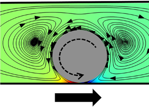
Figure 9. (a) Schematic depiction of the pressure gradient between the fore and aft of the sphere, the directions of rolling and sliding motion, and the streamlines around the sphere for  $R_{ch}/R_s=1.6$ and $\bar {\rho }_s=0.9$. (b) The pressure distribution along the arc shown with the gold dashed line in (a) for $R_{ch}/R_s=1.6$ at selected $\bar {\rho }_s$. The inset shows the $\bar {p}$ distribution for $\bar \rho _s \leq 0.9$. (c) The magnitude of the pressure gradient $\Delta \bar {p}$ with respect to the non-dimensional proximity parameter $\bar {\delta }$. (d,e) are similar to (b,c) but $\bar {\tau }$ and $\bar {\tau }_{max}$ are plotted instead. The dotted lines in (c,e) depict a line with slope $-0.5$ at logarithmic scale.
Looking at the shear stress distribution along the bottom arc (the non-dimensional shear stress is denoted as  $\bar {\tau }$), plotted in figure 9(d), a striking dip is observed right at the bottom of the sphere. This could be explained by the flow reversal in the back and front of the sphere, as shown by the streamlines in figure 9(a). Shear rates go through a maximum at the edges of the nip region due to the flow reversal. The dip in $\bar {\tau }$ disappears completely when the sphere is sufficiently far from the wall, at $\bar {\rho }_s=0.2$. The maximum shear $\bar \tau _{max}$ at low $\bar {\delta }$ (shown in figure 9e) exhibits a trend similar to that of $\Delta \bar {p}$, albeit that the magnitude is an order of magnitude lower for a given $\bar \delta$. Also note that the slope is smaller than the value of $-0.5$ observed for the pressure gradient; it comes out as $-0.833$.
3.3. Experiment results
This subsection reports the velocities of the magnetically rotated spheres from our experiments. The spheres are observed to be ‘rolling’, i.e. translating in the positive  $z$ direction as they are rotated counter-clockwise about the $\beta$ axis when $R_{ch}/R_s=3$, as sketched in figure 9(a). Translation in the opposite of the rolling direction, which is referred to as ‘sliding’, occurs as a response to counter-clockwise rotation about the $\beta$ axis when $R_{ch}/R_s=1.6$, also shown in figure 9(a).
Values of  $u_z$ for the experiments with $R_{ch}/R_s=3$ are plotted against the rotation frequency, $f$, in figure 10(a,b). Fluids with two different viscosities, $\mu =0.5$ Pa s and $\mu =1$ Pa s, and spheres with diameters $D_s=1$ mm and $D_s=1.9$ mm, are tested. When $D_s=1$ mm, $D_{ch}=3$ mm and $\mu =1$ Pa s, $u_z$ increases linearly with increasing $f$ up to 8 Hz (figure 10a). As the rotation frequency is increased beyond this value, the sphere fails to rotate synchronously with the rotating magnetic field, thus the sphere velocity decreases with increasing $f$ up to 20 Hz. Step-out also causes large deviations in $u_z$, as shown by the error bars in the plots, which denote the standard deviation values. The fluctuations in $u_z$ outside the step-out regime can be explained easily by the roughness of the spheres, which leads to a time-varying $\delta$ that alters the resistance coefficients (Smart et al. Reference Smart, Beimfohr and Leighton1993). The step-out frequency and translation velocities are higher overall for the $D_s=1.9$ mm and $D_{ch}=5.7$ mm configuration (10b), owing to the stronger magnetization and increased weight of the sphere that improves the traction. $u_z$ values for $\mu =1$ Pa s and $\mu =0.5$ Pa s are more or less similar up to $f=3$ Hz at both geometric configurations (shown in the insets), but they deviate at larger $f$.
$f$.

Figure 10. Change in  $u_z$ with respect to $f$ for the magnetically rotated spheres in various configurations. The configurations are: (a) $D_s=1$ mm, $D_{ch}=3$ mm; (b) $D_s=1.9$ mm, $D_{ch}=5.7$ mm; (c) $D_s=1$ mm, $D_{ch}=1.6$ mm; and (d) $D_s=1.9$ mm, $D_{ch}=3$ mm. The red lines passing through $u_z=0$ are placed to highlight the transition from rolling ( $u_z>0$) to sliding ( $u_z<0$). The error bars indicate the standard deviation values.
Values of  $u_z$ for the experiment configurations with sliding ( $R_{ch}/R_s=1.6$) are displayed in figure 10(c,d). The red lines passing through $u_z=0$ highlight the transition from rolling (i.e. $u_z>0$) to sliding (i.e. $u_z<0$). The transition to sliding occurs at very low $f$ (around 0.5 Hz) for $\mu =0.5$ Pa s, as shown in the insets. At low frequencies, having a considerable roughness at the surface, spheres establish contact with the wall and roll slowly due to traction. Note that such a motion occurs in only a very small number of experiments. Contact of the roughness elements with the channel boundary could induce a lift that would deter the traction and cause sliding, but the lift appears to be limited as the sphere is able to maintain rolling motion, whereas at higher rotation frequencies the traction is lost and the pressure difference leads to a sliding motion. The variations in $u_z$ with respect to $f$ are mostly linear at the sliding region. Note the overall increases in the magnitudes of the maximum velocities attained before step-out in comparison to $u_z$ observed in rolling spheres. The increase is particularly notable as the viscous effects at narrower channels are expected to be more restraining against motion, as implied by the resistance coefficients reported in § 3.2. The enhanced swimming speeds are due to the large $\Delta \bar {p}$ that contributes to the sliding of the sphere as opposed to rolling, where $\Delta \bar {p}$ hinders the sphere motion.
The experiment results can also be compared with the velocities evaluated from the resistance coefficients with (3.6). This simple calculation means that several types of forces will be neglected. Unsteady forces, such as the history force and added mass forces, are known to play an important role in the swimming of micro-organisms. Jakobsen (Reference Jakobsen2001) reports that Balonion comatum, a ciliate plankton, increases its velocity fivefold in a time period shorter than the time needed to advance the organism more than one body length. Such motions create unsteady disturbances in the flow field that can affect the velocity and trajectory of the swimmers even after the motion causing the disturbance ceases. However, in the scope of the study reported here, these unsteady forces can be neglected, as the density of the particle used in this study is not comparable to the density of the fluid used in the experiments (Van Aartrijk & Clercx Reference Van Aartrijk and Clercx2010). Wang & Ardekani (Reference Wang and Ardekani2012) model a spherical unsteady swimmer and show that the Boussinesq–Basset history term and the added mass term can be neglected when the product of Strouhal ( $Sl$) and Reynolds numbers is smaller compared to unity:
 \begin{equation} \boldsymbol{F}_{hist}+\boldsymbol{F}_{mass} \rightarrow 0,\quad Sl\,Re=\frac{(0.5m_f+m_s)2{\rm \pi} f}{6 {\rm \pi}\mu R_s} \ll 1. \end{equation}
Here,  $m_s$ is the mass of the swimmer and $m_f$ is the mass of the fluid displaced by the swimmer. In this study, the highest $Sl\,Re$ that occurs throughout the experiments is 0.1886, which is achieved when $\mu =1$ Pa s, $f=20$ Hz and $R_s=0.95$ mm. However, as this rotation frequency is above the step-out frequency, above which the sphere rotation loses its synchronization with the rotating magnetic field, the rotation rate of the sphere does not reach 20 Hz at all. Therefore, the actual $Sl\,Re$ value for this configuration is below 0.1886. Thus the effects of history and added mass can be discarded safely.
A critical omission in this approach is the roughness of the sphere, which would bring about a time-varying  $\bar {\delta }$ that would lead to time-varying resistance coefficients as reported in Galvin et al. (Reference Galvin, Zhao and Davis2001). The roughness causes non-continuous traction of the sphere on the surface of the channel, which is highly critical for rolling motion. Note $\delta$ in the experiments cannot be determined as accurately as needed due to the limitations in our image processing capabilities. With $\bar {\delta }$ being unknown, the calculation in (3.6) is carried out for multiple $\bar {\delta }$.
Another consideration would be the effect of the lift force on the sphere. There exist an extensive number of studies investigating the lift force on spheres at low Reynolds numbers (Saffman Reference Saffman1965; Cox & Brenner Reference Cox and Brenner1968; Ho & Leal Reference Ho and Leal1974; Vasseur & Cox Reference Vasseur and Cox1976; Cox & Hsu Reference Cox and Hsu1977; Drew Reference Drew1988; McLaughlin Reference McLaughlin1993; Cherukat & McLaughlin Reference Cherukat and McLaughlin1995), but these studies either do not fit into our configuration or cannot be implemented due to their nonlinear nature. Other models for spheres swimming in bulk or at higher Reynolds numbers point to a strong correlation between an increase in lift force with increasing angular velocity. Lift force is reported to affect  ${\delta }$, and a relevant example would be the study by Bhattacharya, Gurung & Navardi (Reference Bhattacharya, Gurung and Navardi2013), where the authors report equilibrium radial positions (where the inertial lift is balanced by the rest of the hydrodynamic forces) for the spheres inside cylinders with respect to the curvature ratio. Nonetheless, the lift induced by the roughness elements on the spheres appears to be more significant as the inertial lift force should be very low considering the Reynolds number of the system.
Experiment results and calculated  $u_z$ values for multiple $\bar {\delta }$ values are plotted in figure 11 with respect to $f$ up to step-out frequencies for each case. Resistance coefficients for $\bar {\delta }=0.002$ and $\bar {\delta }=0.0006$ (where $\bar \rho _s>0.99$) are evaluated with the FEM model (only the necessary terms), while the coefficients for $\bar {\delta }=0.01$ and $\bar {\delta }=0.003$ are interpolated using piecewise cubic spline interpolation. The results for the $D_s=1$ mm and $D_{ch}=3$ mm configuration (figure 11a) show that $\bar {\delta }$ is between 0.01 and 0.002 in experiments, whereas in $D_s=1.9$ mm and $D_{ch}=5.7$ mm configuration (figure 11b) the experiment values fall between the $u_z$ values for $\bar {\delta }=0.02$ and $\bar {\delta }=0.01$, which indicates that the gap for the larger sphere in the larger channel is higher. Either way, the sphere appears to be very close to the boundaries and rolls along with the help of the traction. For both of the sliding configurations (figure 11c,d), $u_z$ in experiments are between the results for $\bar {\delta }=0.006$ and $\bar {\delta }=0.003$. The sphere is still close enough to get traction, but $\Delta p$ is so great that it results in sliding motion. Galvin et al. (Reference Galvin, Zhao and Davis2001) state that the average $\delta$ between the sphere and the boundary should be between the smaller and larger roughness sizes, so these fits give an estimate for the average roughness element sizes, giving 1–5 $\mathrm {\mu }$m for the sphere with $D_s=1$ mm, and 9.5–19 $\mathrm {\mu }$m for the sphere with $D_s=1.9$ mm, in dimensional terms. The scale of the values with respect to sphere radii is in agreement with what Smart et al. (Reference Smart, Beimfohr and Leighton1993) report. Also worth noting is that the values of $u_z$ fit to different $\bar {\delta }$ values at low and high $f$ values, meaning that $\delta$ is higher at larger $f$. This is consistent with the Galvin et al. (Reference Galvin, Zhao and Davis2001) report where the authors state that a faster rotating sphere would have its large roughness elements making contact with the boundaries more frequently, which results in a larger $\delta$ in average. Finally, note that the estimated sizes of average roughness elements are of the order of the gap sizes reported for cavitation in Appendix E, therefore it is possible that cavitation might have occurred but we do not expect it to be significant compared to the effects caused by the roughness elements.

Figure 11. Comparison of  $u_z$ from experiments with the velocities obtained from the resistance coefficients for (a) $D_s=1$ mm, $D_{ch}=3$ mm; (b) $D_s=1.9$ mm, $D_{ch}=5.7$ mm; (c) $D_s=1$ mm, $D_{ch}=1.6$ mm; and (d) $D_s=1.9$ mm, $D_{ch}=3$ mm. Insets show $u_z$ for small $f$.
$f$.
Sliding and rolling velocities of the sphere are higher in magnitude in the higher viscosity fluid than the ones in the lower viscosity fluid. This indicates that the sphere's distance to the wall,  $\delta$, is larger during sliding at the more viscous fluid, but also that $\delta$ is smaller during rolling at the more viscous fluid. It is not clear why such a dichotomy occurs in the results. Furthermore, the competing effects, pressure and viscous forces, scale linearly with $\mu$ at the Stokes regime, thus there should be no difference with respect to $\mu$ in sphere motion. For sliding, the roughness elements appear to deter the traction. As reported by Galvin et al. (Reference Galvin, Zhao and Davis2001), when a large roughness element on the sphere makes contact with the boundary, the sphere is temporarily lifted off from the surface. In a more viscous fluid, it would take more time for the gravitational forces to pull the sphere down to lower $\delta$. That is why $u_z$ is higher in magnitude with the more viscous fluid and also why $u_z$ data for large $f$ from the experiments fit better to the velocity profile for the larger $\delta$. For rolling, the roughness elements appear to improve the traction of the sphere with increasing viscosity, thereby decreasing $\delta$. A second possibility would be that in the high viscosity case, pressure may drop to a level that causes evaporation in the silicon oil, limiting the minimum pressure to vaporization pressure, which is very small for silicon oil. On the other hand, the high pressure in the nip region is not bounded, thus pressure forces may not cancel and a net pressure force may lead to the levitation of the sphere. However, the analysis in Appendix E indicates that no cavitation should occur. In our numerical analysis, we could not confirm the presence of a lift force on the rotating sphere with or without the inertial forces. Therefore, the trend appears to be related to the roughness elements on the sphere.
4. Conclusion
Motion of rotating spherical particles in cylindrical conduits is investigated here numerically and experimentally. For the first time, a unique experiment set-up is used to demonstrate the rolling and sliding behaviour of magnetically rotated spheres inside cylindrical channels filled with a viscous fluid. Elements of the resistance matrix are calculated using a validated finite-element model with a lower computational cost than analytical models, especially for the case when the motion of a single sphere very close to the channel wall is considered. The resistance coefficients are reported for different confinement ratios and a range of radial positions, with a special focus on the motion in close proximity to the channel boundaries.
Resistance and coupling coefficients in the resistance matrix are used to study the rolling and sliding phenomena. A near-wall rotating sphere slides along the channel for small confinement ratios due to the very high pressure gradient in the nip region between the channel and the sphere, whereas the shearing forces are dominant in rolling observed for larger confinement ratios. Another interesting finding is that a flow reversal causes a dip in the shear stress in the nip region.
In the experiments, radially magnetized spherical magnets are placed in viscous fluid-filled horizontal cylindrical channels. Due to their weight, spheres are observed to be resting on the channel wall. When the spheres are rotated in the azimuthal direction with the help of a rotating magnetic field, sliding motion is observed along the channel in the opposite direction to the rolling direction at high confinement ratios owing to the pressure buildup near the nip region between the sphere and the channel. It is shown that the pressure gradient has similar magnitudes in different confinement ratios for a given non-dimensional gap size between the sphere and the channel. This would imply that sliding should be possible at all confinement ratios, but the differences in resistance coefficients at different confinement ratios prevent this from happening.
In the experiments, sliding is observed for the confinement ratio 1.6, whereas rolling is observed for the confinement ratio 3 for both viscosity values. Sliding velocities are larger in magnitude than the rolling velocities for a given magnetic rotation frequency as the sphere has to overcome the pressure gradient in the rolling motion whereas the sphere is pushed by the pressure gradient in the sliding regime. Translation velocities evaluated from the resistance coefficients for the experiment configurations indicate that the sphere is very close to the channel boundaries in both swimming modes. The proximity to the wall cannot be predicted accurately due to both image processing limitations and the roughness of the spherical surface. In small confinement ratios, rolling can take place at very low rotation rates, but as the rotation rate increases, a transition from rolling to sliding occurs. Surface roughness of the sphere causes a lift-off from the channel boundaries that affects the average gap size between the channel wall and the sphere, leading to fluctuations in the axial velocity and loss of traction that is critical for rolling, and also larger axial velocities at more viscous fluids. Faster rotation rates of the sphere amplify the effects of the surface roughness, increasing the gap size as evidenced by the evaluated velocities from the resistance coefficients. Overall, the findings of this study are expected to improve understanding on the motion of spherical particles in cylindrical channels, which is of interest from different perspectives in fluid mechanics. For a specific example, results could prove useful to study magnetic spherical particles as micro robots in cylindrical conduits in microfluidic applications.
Acknowledgements
The authors would like to thank Professor S. Bhattacharya for sharing code for the model in Bhattacharya et al. (Reference Bhattacharya, Mishra and Bhattacharya2010) and extensive discussions.
Data availability statement
The data that support the findings of this study are provided in the appendices. Further data are available upon reasonable request.
Declaration of interests
The authors report no conflict of interest.
Appendix A. Measurements on the roughness of the spheres used in the experiments
We report the roughness measurements for the spheres used in the experiments here. A Nanofocus 3-D surface metrology system is used for the measurements. Figure 12(a) shows a close-up image of the sphere with  $D_s=1$ mm, while figure 12(b) shows the roughness surface plot for the same sphere. The surface height distribution for the same sphere is provided in figure 12(c). According to the measurements carried out at ISO 4287 standards, the $Rt$ parameter comes out as 8.56 $\mathrm {\mu }$m, while $Ra=1.16$ $\mathrm {\mu }$m. A large $Rt/Ra$ ratio indicates that the surface has significant dips or peaks along the measured profile, and for this sphere the ratio comes out as 7.37. The sphere with $D_s=1.9$ mm exhibits lower roughness, with an $Rt/Ra$ ratio of 3.68. A ratio of 1 would indicate that there are no significant dips and peaks that go further beyond the average roughness on the surface.

Figure 12. (a) Close-up image of the magnetic sphere with  $D_s=1$ mm used in the experiments. (b) Surface height distribution measurement results for the sphere with $D_s=1$ mm. (c) Surface profile measurement of a part of the same sphere.
Appendix B. Complete list of resistance coefficients
The complete list of the resistance coefficients in normalized form is provided here. Table 2 lists the coefficients for  $R_{ch}/R_s=1.6$, table 3 lists the coefficients for $R_{ch}/R_s=2$, and table 4 lists the coefficients for $R_{ch}/R_s=3$. Refer to (2.5) for the definition of $\bar \rho _s$, and to (3.1)–(3.4) for the normalization equations.
Table 2. The resistance coefficients for  $R_{ch}/R_s=1.6$.

Table 3. The resistance coefficients for  $R_{ch}/R_s=2$.

Table 4. The resistance coefficients for  $R_{ch}/R_s=3$.

Appendix C. Comparison of the resistive coefficients with the results from the literature
This section contains figures comparing the resistance coefficients obtained from the FEM model and the Bhattacharya et al. (Reference Bhattacharya, Mishra and Bhattacharya2010) code. Figures 13 and 14 show the plots for  $R_{ch}/R_s=1.6$, and figures 15 and 16 show the comparisons for $R_{ch}/R_s=3$.

Figure 13. Comparison of the translational and rotational resistance coefficients obtained from the FEM simulations and the data in the literature for  $R_{ch}/R_s=1.6$. (a) $\bar {F}^{tt}_{\rho \rho }$, (b) $\bar {F}^{tt}_{\beta \beta }$, (c) $\bar {F}^{tt}_{zz}$, (d) $\bar {F}^{rr}_{\rho \rho }$, (e) $\bar {F}^{rr}_{\beta \beta }$ and ( f) $\bar {F}^{rr}_{zz}$. The insets show the coefficients for $\bar \rho _s\geq 0.9$.

Figure 14. Comparison of the coupling resistance coefficients obtained from the FEM simulations and the data in the literature for  $R_{ch}/R_s=1.6$. (a) $\bar {G}$ and (b) $\bar {G}'$. The insets show the coefficients for $\bar \rho _s\geq 0.9$.

Figure 15. Comparison of the translational and rotational resistance coefficients obtained from the FEM simulations and the data in the literature for  $R_{ch}/R_s=3$. (a) $\bar {F}^{tt}_{\rho \rho }$, (b) $\bar {F}^{tt}_{\beta \beta }$, (c) $\bar {F}^{tt}_{zz}$, (d) $\bar {F}^{rr}_{\rho \rho }$, (e) $\bar {F}^{rr}_{\beta \beta }$ and ( f) $\bar {F}^{rr}_{zz}$. The insets show the coefficients for $\bar \rho _s\geq 0.9$.

Figure 16. Comparison of the coupling resistance coefficients obtained from the FEM simulations and the data in the literature for  $R_{ch}/R_s=3$. (a) $\bar {G}$ and (b) $\bar {G}'$. The insets show the coefficients for $\bar \rho _s\geq 0.9$.
Appendix D. Convergence study on the Bhattacharya et al. (Reference Bhattacharya, Mishra and Bhattacharya2010) model
A convergence study over  $l_{max}$ for the Bhattacharya et al. (Reference Bhattacharya, Mishra and Bhattacharya2010) model is presented in figure 17. For reference, the FEM results are given by dashed lines in the same figure. The rotational coefficients exhibit reasonable accuracy at all $l_{max}$, while $\bar {F}^{tt}_{\rho \rho }$, $\bar {G}$ and $\bar {G}'$ require large $l_{max}$ to converge. Note that the Bhattacharya et al. (Reference Bhattacharya, Mishra and Bhattacharya2010) BTSM model results are also dependent on the parameters $\mu _{max}$, $\varLambda _{max}$ and $\delta _\lambda$, and a multi-parameter convergence study is required to achieve complete convergence. The BTSM results are expected to fully match our FEM results once multi-parameter convergence is achieved. In this study, we limit ourselves to a set of parameters that exhibit sufficient convergence (parameters given in § 3.1). Multi-parameter convergence of BTSM in close proximity is outside the scope of this study, and it is noted for future work.

Figure 17. Convergence of the resistance coefficients in the Bhattacharya et al. (Reference Bhattacharya, Mishra and Bhattacharya2010) model for  ${R_{ch}/R_s=2}$ and $\bar \rho _s=0.99$. (a–c) The translational resistances; (d–f) the rotational resistances; (g,h) the coupling resistances. Finite-element results are shown with dashed lines.
Appendix E. On cavitation in the flow
This appendix provides estimations on the cavitation conditions in the flow. The vapour pressure of silicone oil at 25 $^\circ$C is reported to be 5 mmHg, which converts to 666.61 Pa at maximum for a kinematic viscosity level of 1000 cSt that corresponds to a dynamic viscosity of 0.97 Pa s (Merck KGaA 2021). In our simulation model, we apply a pressure point constraint at the end of the tube, with reference pressure 0. Figure 9(b) shows that the non-dimensional pressure level goes down to $-1578$ at the tightest configuration tested in the scope of this work for $\bar {\delta } < 0.006$. Dimensionalizing this value requires $\mu$ and $f$. The largest $\mu =1$ Pa s and $f=20$ Hz give $p=\bar {p}\mu f=-31\,560$ Pa. Considering that our reference is atmospheric pressure, $10^5$ Pa, we observe a minimum absolute pressure of 68 440 Pa, much bigger than the vapour pressure for the silicone oil. However, cavitation may occur at closer distances under those conditions ( $\mu =1$ Pa s, $f=20$), at $\bar {\delta } < 0.0027$, or $\delta < 2.7$ $\mathrm {\mu }$m. For a smaller frequency, $f=10$ Hz, for which we assume a synchronous rotation of the sphere with the magnetic field, the gap thickness for which cavitation is expected would be smaller, i.e. $\bar {\delta } < 0.0019$, or $\delta < 1.9$ $\mathrm {\mu }$m.


 Open access