


1. Introduction
The flow field and drag force generated by a rising rigid sphere in a rotating fluid are of practical and academic interest. The applications vary from the cores of planets to biological centrifuges. The theory is concerned with subtle structures like the Ekman and Stewartson shear layers, and the fascinating long Taylor column. These problems are characterized by a peculiar difficulty: apparently, there are significant discrepancies between the measured drag force and theoretical predictions. In this respect, it is essential to distinguish between ‘long’ and ‘short’ containers. In the first case (compared with the diameter of the sphere), long detached conical Taylor columns appear in front of and behind the sphere, and the measured drag is typically larger than the theoretical predictions; see the recent paper by Aurégan, Bonometti & Magnaudet (Reference Aurégan, Bonometti and Magnaudet2023), and the references therein. Here, we consider the second case, in which the flow is structured as  $z$-independent cylindrical columns (cores) attached to the sphere and governed by the Ekman layers on the bounding plates of the container and on the sphere (where $z$ is the axis of rotation). The typical height of the column is just a few diameters of the particle. The classical measurements of Maxworthy (Reference Maxworthy1968) and the recent measurements of Kozlov et al. (Reference Kozlov, Zvyagintseva, Kudymova and Romanetz2023) found a significantly smaller drag than predicted by the classical geostrophic solution of Moore & Saffman (Reference Moore and Saffman1968, Reference Moore and Saffman1969). The studies of Maxworthy (Reference Maxworthy1968) and Kozlov et al. (Reference Kozlov, Zvyagintseva, Kudymova and Romanetz2023) will be referred to as Max68 and K23, respectively.
This paper revisits the problem of the drag discrepancy and the attempts for interpretation and improvement. Our work is novel in several aspects. First, we use the combined data of two independent parties, Max68 and K23, that differ in time, methodology and apparatus. This increases the parameter range and improves the overall reliability. Second, we reprocess the data ‘from scratch’ (as much as possible) in a form that is more straightforward for insights and comparisons. Third, we make comparisons with a wider range of theoretical predictions, significantly beyond the geostrophic solution. In particular, we emphasize the strong connection between the angular velocity in the cores and the drag force. The novel analysis leads to the rejection of the suggestion that inertial effects are the reason for drag discrepancy. We demonstrate that the reason is the vertical Stewartson layers (not included in the geostrophic drag result), and derive a semi-empirical drag correction that agrees well with the data. We also consider curve-fit formulas and point out their limitations.
We note in passing that various extensions of this problem have been considered in the literature, e.g. Bush, Stone & Bloxham (Reference Bush, Stone and Bloxham1992, Reference Bush, Stone and Bloxham1995) considered a drop with a non-rigid surface, and Ungarish & Vedensky (Reference Ungarish and Vedensky1995) and Minkov, Ungarish & Israeli (Reference Minkov, Ungarish and Israeli2000) solved the problem for a rising disk. These works strengthen the theoretical understanding of the flow, but do not contribute to the clarification of the discrepancy considered in this paper.
The structure of the paper is as follows. Fundamental concepts and theoretical results are presented in § 2, followed by a brief report of the theoretical balances and drag calculation formulas that will support the comparisons with the data in § 3. Comparisons are performed and discussed in § 4. Here, we explain the difficulties of the sets of data used in our work. The comparison of the angular velocity suggests a semi-empirical correction of the drag calculations. Detailed comparisons of the drag are performed next. Concluding remarks are given in § 5. Curve-fit formulas are discussed in Appendix A.
2. Fundamental concepts and results
We consider a solid spherical particle of radius  $a$ and density $\rho _p$ in a homogeneous fluid of density $\rho \ (>\rho _p)$ and kinematic viscosity $\nu$ in a system rotating with constant angular velocity $\varOmega$ about the vertical axis $z$. The particle moves with a quasi-constant velocity $W$ along the vertical axis $z$ (upwards), opposite the gravity acceleration $g$. The fluid fills a co-rotating cylinder with solid horizontal lids (plates). The dimensionless parameter $H$ expresses the ratio of the height of the cylinder to $2a$ (the diameter of the particle). We assume that the particle is at the midplane between the top and bottom plates (the relevance of this situation to other positions is discussed in Appendix B). See figure 1.

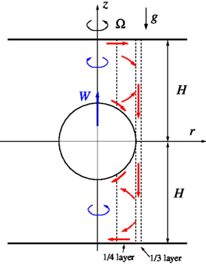
Figure 1. Sketch of the flow field, sphere in symmetric position. In the upper side, the fluid is transported outwards in the Ekman layers and  $1/4$ Stewartson layer, then downwards in the $1/3$ layer. The decrease of the volume is compensated by the upward motion of the sphere with velocity $W$. The system of coordinates co-rotates with the plates at rate $\varOmega$. The cores display azimuthal velocity $v(r)$ relative to the system (negative in the upper side). In general, a $1/4$ layer appears also on the outer side of the $1/3$ layer, but in the symmetric position, this layer is not needed, and therefore not shown. The outer wall of radius $r_O$ is not shown, and is unimportant under the assumption that the gap from the sphere is larger than the $1/3$ and $1/4$ layers. Here, $H$ is normalized with the radius of the sphere, $a$.
$a$.
We are concerned with the drag  $D$ on the particle. The quasi-steady state $W$ implies equilibrium with the known buoyancy
 \begin{equation} B = \tfrac{4}{3} {\rm \pi}\rho a^3g',\quad g' = (1- \rho_p/ \rho) g \end{equation}
(where  $g'$ is called reduced gravity). Measuring $W$ for a known $D=B$ in an experiment is formally a straightforward task: set $g'$, release the particle near the bottom in the rotating fluid, and record the trajectory (only results that show a steady-state are relevant). The question that is the backbone of this paper is: what is the connection between $D$ and $W$? In other words, we are concerned with the prediction of $D$ as a function of $W$, and the understanding of the mechanisms that govern the result. Obviously, this must depend on the dimensionless parameters of the flow.
The major parameters are
 \begin{equation} T = E^{-1} = \frac{\varOmega a^2}{\nu},\quad Ro = \frac{W}{\varOmega a}, \end{equation}
where  $T$ is the Taylor number, $E$ is the Ekman number and $Ro$ is the Rossby number. For later reference, we define the dimensionless parameters
 \begin{equation} \varepsilon = (H/2)^{1/2} T ^{-1/4},\quad \varepsilon_{1/3} = H^{1/3} T ^{-1/3}, \end{equation}
which are the typical dimensionless thicknesses (scaled with  $a$) of the Stewartson layers discussed later.
We are concerned with small  $Ro$ and large $T$, which is regarded as a flow field with strong rotation and small viscous effects (confined to thin layers). Such flows display the Taylor–Proudman columnar structure, in the sense that the moving particles induce significant motion in columns ahead and behind. In this respect, two different types of flow must be distinguished. In the long container, $H> T/20$ (approximately), the major part of the Taylor column is a free domain of recirculation, of conical shape. In the short container, $1.5 < H < T ^{1/2}$ (approximately), the Taylor column is a cylinder of radius $a$ in which the pressure, radial velocity and angular velocity are independent of $z$, called quasi-geostrophic flow. (In the case $H<1.5$, the vertical gap at the centre is less than half-radius. Although no qualitative failure of the quasi-geostrophic theory is expected as long as the gap admits Ekman layers, i.e. for $H > 1+ 6/T^{1/2}$, the small gap requires a reconsideration of the matching between the inviscid core and the viscous layers. This uncertainty is avoided by the $H>1.5$ restriction.)
The different ‘long’ and ‘short’ quasi-steady flow regimes emerge from the boundary conditions during the time-dependent process of formation. Initially (time  $t=0$), the sphere is at rest and the fluid is in solid-body rotation. The rotating fluid supports inertial waves. The beginning of the motion of the sphere along the axis generates waves. Consider the upper $z>0$ domain (the lower domain is symmetric). The waves produce a (Taylor) column of increasing length, ${\sim }0.7 \varOmega a t$; see § 4.3 of Greenspan (Reference Greenspan1968), and Minkov, Ungarish & Israeli (Reference Minkov, Ungarish and Israeli2002). The small viscous forces in the perturbed fluid tend to block this propagation, but this can be achieved over a distance ${\sim }a T/ 20$. In the ‘long’ container, the top boundary of the container is sufficiently far away, and this arrested column evolves into a steady state. In the ‘short’ container, the wave hits the top plate at an early stage, is reflected, and activates the viscous reaction of the solid boundaries (the Ekman layers). The adjustment to steady state is then performed by the more conventional spin-up process dominated by the Ekman layers. For a sufficiently small $Ro$, the time scale of the axial motion, $H/(Ro \varOmega )$, is much longer than that of the initial adjustment, and this justifies a steady-state analysis of the flow.
In this paper we will focus attention on the short container case only. We will show that this case, although apparently simple due to the  $z$-independent core, lacks an assessed theory, and poses some questions that indicate the need for new experiments and simulations.
Three viscous layers appear in the problem. We use the radius of the sphere  $a$ as the reference length for the discussion of these layers. Ekman layers of typical thickness $T^{-{1/2}} = E^{1/2}$ connect the vertical core with the particle on one side and with the lid on the other side; these are called ‘horizontal layers’. Stewartson layers of thickness $\varepsilon = (H/2)^{1/2} T^{-1/4}$ embed the core in both inner $r<1$ and outer $r>1$ directions. A Stewartson layer of typical thickness $\varepsilon _{1/3} =H^{1/3} T ^{-1/3}$ is sandwiched between the $1/4$ layers. For obvious reasons, these are also called the $1/4$ and $1/3$ (vertical) layers.
The theory is based on  $Ro \to 0$ approximation (called linear theory; Greenspan Reference Greenspan1968) and $T \to \infty$ (thin viscous layers). Some details are given in § 3. The axisymmetric Navier–Stokes equations are simplified using an expansion of the dependent variables in powers of $Ro$ and $1/T$. The matching of the leading terms produces the following main results for the drag.
(1) The geostrophic result (Moore & Saffman (Reference Moore and Saffman1968) assuming $\varepsilon \to 0$) is explicit:
(2.4)\begin{equation} D_0 = \frac{43}{105} {\rm \pi}T^{3/2} \times (W \nu \rho a) = 1.29 T^{3/2} (W \nu \rho a). \end{equation}
$\varepsilon \to 0$) is explicit:
(2.4)\begin{equation} D_0 = \frac{43}{105} {\rm \pi}T^{3/2} \times (W \nu \rho a) = 1.29 T^{3/2} (W \nu \rho a). \end{equation}(2) The quasi-geostrophic (qg) result for a particle in the middle of the cylinder (Ungarish (Reference Ungarish1996) assuming finite
$\varepsilon$ but $\varepsilon _{1/3} \to 0$) is given implicitly as
(2.5)\begin{equation} D_{qg} = \mathcal{D}(\varepsilon, H)\,T^{3/2} \times (W \nu \rho a). \end{equation}


Here,  $\mathcal {D}$ is of the order of unity, typically smaller than 1.29. The value of $\mathcal {D}$ is obtained by standard numerical methods. The quasi-geostrophic results are amenable to some extensions: non-middle position of the particle, nonlinear corrections (finite small $Ro$), and dependency on the time $t$. These extensions provide useful insights concerning the trends of these effects, but the addition of parameters ( $Ro, H_u/H_l, t$) to the theory complicates the discussion and will not be presented here. We restrict our comparisons to the results of the simple steady-state quasi-geostrophic result for $H=H_u$, $H_u/H_l =1$, $Ro =0$. The subscripts $u,l$ denote the upper and lower domains of the flow.
The convenient connection between theory and experiments is via the dimensionless  $D/D_0$, where $D$ is the measured drag for a given set of parameters and $W$.
$W$.
Conversely, suppose that the buoyant force on the sphere,  $B$, is known (this is easy to calculate or measure). Letting $B=D_0$ (see (2.1) and (2.4)), we obtain the geostrophic axial velocity
 \begin{equation} W_0 = \frac{140}{43} \left( \frac{g' a^2}{\nu}\right ) T ^{-3/2} = 3.26 \left (\frac{g' a^2}{\nu} \right ) T ^{-3/2}. \end{equation}
Since the drag is proportional to  $W$, we can write for a given experimental point
 \begin{equation} \frac{W}{W_0} = \frac{D_0}{D}, \end{equation}
which means that the measurement of the speed  $W$ provides an excellent assessment for the accuracy of the drag prediction.
For compatibility with the literature, we also introduced the drag coefficient  $c_D = 2 D/(\rho {\rm \pi}a^2 W^2)$, the Reynolds number $Re = W a / \nu$, and the settling Reynolds number $\psi = (g' a^2/\nu )(a/\nu )$. Some algebra yields the relationships
 \begin{equation} c_D = \frac{86}{105}\,\frac{T^{1/2}}{Ro}\,\frac{D}{D_0},\quad \psi = \frac{43}{140}\,Ro\,T^{5/2}\,\frac{D}{D_0},\quad Re = Ro\,T. \end{equation}
3. Theory
We recall briefly some essential theoretical results, following Ungarish (Reference Ungarish1996); see figure 1. The cylindrical system of coordinates is attached to the centre of the sphere and co-rotating with the horizontal plates (lids) at constant angular velocity  $\varOmega$. Gravity acts in the $-z$ direction, while the particles move with speed $W$ in the opposite direction. The flow is axisymmetric and unbounded in the radial direction. Ekman layers are present on the sphere and horizontal plates. The typical thickness of the Ekman layer is
 \begin{equation} \delta = (\nu / \varOmega)^{1/2} = a T^{-{1/2}}. \end{equation}
The sphere is given by
 \begin{equation} z ={\pm} a\,f(r), \quad f = (1-\xi^2)^{1/2}, \quad \xi = r/a, \end{equation}
while the position of the plates is  $\pm a H$. (Again, $H$ is dimensionless.)
In the cores of fluid between the Ekman layers, the radial velocity  $u$, azimuthal velocity $v$ and (reduced) pressure $p$ are $z$-independent. Due to the symmetric position of the sphere, the flows in the upper and lower sides are antisymmetric, and the torque on the sphere vanishes. This means that the sphere is co-rotating with the plates, and it is sufficient to solve the flow in one domain. (The symmetry condition can be relaxed by applying matching conditions between the cores, but this is beyond the scope of this paper.) Let us focus attention on the upper side.
Consider first the volume conservation. We use a cylindrical control volume of radius  $r< a$ between $z = a\,f(r)$ and $z = a H$. Fluid flows out via the core and via the Ekman layers at the rate
 \begin{equation} Q(r) = 2 {\rm \pi}r \left(a [ H - f(r) ] u - \tfrac{1}{2} \delta [ 1 + (1 + {f'}^2)^{1/4}] v\right)\!. \end{equation}
This outflux is sustained by the volume compression of the cylinder at the rate  $Q(r) = {\rm \pi}r^2 W$.
Consider next the momentum balances in the core. The dominant acceleration is due to Coriolis. In the  $z$ direction, $\partial p /\partial z =0$ is satisfied by a general $p(r)$. The radial Coriolis term is balanced by the pressure, while the azimuthal Coriolis term is balanced by viscous forces. This reads
 $$\begin{gather} - 2 \varOmega v=- \frac{1}{\rho}\,\frac{{\rm d} p}{{\rm d} r}, \end{gather}$$
 $$\begin{gather}2 \varOmega u = \nu\,\frac{{\rm d}}{{\rm d} r}\,\frac{1}{r}\,\frac{{\rm d}}{{\rm d} r} rv. \end{gather}$$
 Substitution of (3.5) into (3.3) and matching the radial flux with the axial compression, we obtain one equation for the azimuthal velocity  $v(r)$. The symmetry between the upper and lower cores imposes $v_u (r)= - v_l(r)$. Therefore, using (3.4), the drag on the sphere is given by
 \begin{equation} D = 4 {\rm \pi}\int_0^a |p(r)|\,r \,{\rm d} r = 4 {\rm \pi}\rho \varOmega \int_0^a |v|\,r^2 \,{\rm d} r, \end{equation}
where integration by parts was used. (We also used the condition that there is no pressure jump at  $r =a$.)
3.1. The dimensionless angular velocity $\omega$

It is convenient to express the reduced volume and momentum balances in dimensionless form. We scale lengths with  $a$, and velocity with $W$. We introduce the scaled angular velocity
 \begin{equation} \omega(r) = T^{-{1/2}}\,v(r)/r \end{equation}
and the dimensionless  $\varepsilon = (H/2)^{1/2} T^{-1/4}$. After some algebra, the above-mentioned equation for $v(r)$ (obtained by the combination of volume continuity with the azimuthal momentum equation) can be expressed as
 \begin{equation} 2 \varepsilon ^2 (1 - f(r)/H)\left(\frac{{\rm d}^2 \omega}{{\rm d} r^2} + \frac{3}{r}\,\frac{{\rm d} \omega}{{\rm d} r}\right ) - [1+ (1 + {f'} ^2)^{1/4}] \omega = 1 \quad (0 \le r \le 1) \end{equation}
with the boundary conditions  $\omega (1) =0,\ ({\rm d} \omega /{\rm d} r) (0) = 0$. The drag prediction (3.6) is then expressed as
 \begin{equation} D = 4 {\rm \pi}T^{3/2} \int_0^1 (|\omega(r) |)\,r^3 \,{\rm d} r \times (W \nu \rho a). \end{equation}
 The shear term on the left-hand side of (3.8) represents the contribution of the  $1/4$ layer to the outward radial transport of the fluid; the next term represents the contribution of the Ekman layers. The right-hand side of (3.8) represents the upward motion that generates the radial fluxes. Evidently, a negative $\omega$ is needed in the upper core. (For the lower core, not solved here, (3.8) with $-1$ on the right-hand side applies. Therefore $-\omega$ of the upper core is the solution for the lower core.)
For  $\varepsilon = 0$, we obtain analytically the geostrophic solution
 \begin{align} \omega_0(r) =- \frac{(1 - r^2)^{1/4}}{1 + (1 - r^2)^{1/4} }, \quad D_0 = \left(\frac{43}{105}\,{\rm \pi}\right) T^{3/2} \times (W \nu \rho a) = 1.29T^{3/2} (W \nu \rho a). \end{align}
 For a finite  $\varepsilon$, we use a finite-difference solution for (3.8) and (3.9). In this case, we must specify $H$ and $T$ (or $\varepsilon$ and one of these parameters). We obtain, numerically,
 \begin{equation} \omega_{qg}(r; \varepsilon,H),\quad D_{qg} = \mathcal{D}(\varepsilon,H)\,T^{3/2} \times (W \nu\rho a). \end{equation}
We expect  $\omega _{qg}(r)/\omega _0(r) <1$ and $\mathcal {D} < 1.29$. Note the difference between (3.10a,b) and (3.11a,b): the first depends only on $T$; the second predicts a more complex behaviour, because for a given $T$, various values of $\varepsilon$ and $H$ are possible practically.
By setting  $f =0$, the rising disk problem is recovered; in this case, for $\varepsilon \ll 1$, (3.8) reduces to $\varepsilon ^2 \omega '' - \omega = 1/2$, hence
 \begin{equation} \omega_{qg\ disk} =- \tfrac{1}{2} [ 1 - \exp ((r-1)/ \varepsilon) ], \end{equation}
which illustrates the classical Stewartson  $1/4$ layer in this context. When $\varepsilon$ is not very small, curvature terms distort the exponential decay, and the $\omega (1) =0$ boundary condition affects the entire domain, including a reduction of $|\omega (0)|$. For simplicity of discussion, we include this behaviour in the concept of the $1/4$ Stewartson layer. Quantitatively, the numerical solution of (3.8) that is used in our comparisons contains the curvature terms and the effect of non-small $\varepsilon$.
We note that the reduced formulation (3.8) and (3.9) is based on reliable physical balances (Ekman layer transport, volume conservation, momentum equations in radial, azimuthal and axial directions). The simplicity of the result is a consequence of simplifications that can be justified for asymptotic limits of the parameters. The physical relevance of the results is for finite values of  $Ro$,
$Ro$,  $\varepsilon$ and $\varepsilon _{1/3}$. The accuracy of the predictions for realistic values of the parameters must be tested by comparison with realistic data.
4. Comparisons
4.1. Difficulties
The assessment of the theory by the available experiments encounters various difficulties. Formally, experiments for small  $Ro$ are expected to provide $D/D_0$ and also $\omega (r)$, whose dimensionless values are of the order of unity, that can be compared straightforwardly with the theory. A close inspection of the major available data reveals that (1) they do not cover the parameter range needed for a conclusive comparison, and (2) there are uncertainties that cast some doubts on the data.
4.2. The angular velocity $\omega (r)$

It is convenient to start the comparisons with the angular velocity in the cores. There is consensus in the literature that the flow is dominated by the Ekman layers, and this requires that (1) the azimuthal velocity  $v$ is of the order of magnitude $T^{1/2} W$, and (2) $v_u<0$ while $v_l >0$. (Again, $u, l$ denote the upper and lower cores, respectively.) The behaviour of the scaled $v/r$, denoted $\omega$, as a function of the dimensionless $r$, is of interest; see § 3.1.
We note that the comparison concerning the data of  $\omega (r)$ of the fluid in the cores is inconclusive. Few data have been reported, and there is no overlap between Max68 (using die tests) and K23 (using a particle image velocimetry technique).
Figure 10 of Max68 displays data of  $|\omega |$ close to the centre versus $Ro\,T$ obtained with a towed sphere, for $4000< T<16\,000$. The figure provides the following conclusions. (1) As expected, $\omega _u(0)<0$ while $\omega _l(0)>0$. (2) The value $|\omega _u(0)|$ is slightly smaller than $\omega _l(0)$. This observation is surprising, because it contradicts the prediction of the theory and is in contrast with the more detailed measurements of K23. (To understand this effect, the extension of the quasi-geostrophic analysis for finite $Ro$ must be used. Qualitatively, as suggested by figure 1, the advection terms compress $\varepsilon _u$ and enlarge $\varepsilon _l$, therefore $|\omega _u|/\omega _l >1$ is expected.) (3) The typical value of $\omega (0)$ decreases from 0.45 to 0.35 as $Ro\,T$ increases from 7 to 28. The interpretation of this variation is problematic because apparently both $Ro$ and $T$ were varied between the points (no details are provided). Max68 remarks that there was big scatter in these data.
Figure 7 of K23 provides more detailed  $\omega (r)$ information for $T = 2890$ and $Ro = 0.0015$ (approximately). We consider the measurements for a sphere in mid-position (the points with open circle and full diamond in that figure). The digitized and rescaled data of $\omega (r)$ are plotted in figure 2, together with the theoretical predictions (geostrophic, quasi-geostrophic and corrected quasi-geostrophic).

Figure 2. Plots of  $|\omega |$ versus $r$ for $T = 2890$. The lines with symbols are data for the upper and lower cores from K23 figure 7. Also shown are the theoretical results: geostrophic (dotted line), quasi-geostrophic (solid line), and corrected quasi-geostrophic (dash-dotted line).
We note that a quantitative comparison of  $\omega$ data between Max68 and K23 is not possible because of significant incompatibly of $T$ and $r$ position of the reported points. The agreement concerning the signs of $\omega _l$ and $\omega _u$ is a trivial confirmation of the Ekman-layer control of the flow. However, K23 report $|\omega _u| > \omega _l|$, in agreement with the theory (in contrast with Max68). On the other hand, we note that the difference between $\omega _l$ and $|\omega _u|$ reported by K23 is much larger than in Max68. We have no theoretical explanation for this observation. Such a significant asymmetry is expected to produce a torque and thus rotation of the sphere; but figure 4 of K23 indicates no such rotation for a sphere in middle position. We speculate that the $\omega _l$ of the K23 data was contaminated by some instability or measurement problem. We conjecture that the data for $\omega _u$ are correct, and, given the very small $Ro = 0.0015$ of the experiment, a repeated experiment will find a close match in the lower core.
4.2.1. Semi-empirical corrections of $\omega$ and $D$


The  $\omega (r)$ data of K23 throw some light on the theory. Figure 2 indicates a significant discrepancy between the predicted and measured $\omega (r)$ about the cylinder $r=1$. The theory uses the boundary condition $\omega (r = 1) = 0$. The data indicate that this condition is fulfilled at $r \approx 1.3$. We note that a similar shift of the $\omega = 0$ point has been detected theoretically for a disk; see figure 5 of Minkov et al. (Reference Minkov, Ungarish and Israeli2000). We attribute this shift of the $\omega = 0$ condition to the presence of a thick $1/3$ Stewartson layer: here, $\varepsilon _{1/3} = 0.15$. The exact mechanism that connects the Ekman layers to this $1/3$ layer is obscure presently. The theoretical analysis of this flow is expected to be complicated and the results impractical, because small powers of $E=(1/T)$ are involved, and an asymptotic separation of terms can be attained only for extremely large values of $T$ (say $10^{12}$). For progress, we adopt a semi-empirical approach.
Figure 2 suggests that the quasi-geostrophic  $|\omega (r)|$ decreases too sharply to $0$ at $r=1$. A more realistic profile is obtained by a shift of the $\omega = 0$ point to $r = 1 + \varDelta$, where $\varDelta =c (2 H /T)^{1/3}$, and $c$ is a coefficient of the order of 1. (This $1/3$ layer is on the outer side of the sphere, hence the relevant dimensionless height is $2H$, and the thickness is $2^{1/3} \varepsilon _{1/3}$.) Since the shift is due to the Stewartson layer, it should not affect the centre domain. We postulate the corrected profile as
 \begin{equation} \omega_c(r) = \left\{\begin{array}{@{}ll@{}} \omega_{qg}(r=0) & (0 \le r \le \varDelta), \\[3pt] \omega_{qg}(r-\varDelta) & ( \varDelta < r \le 1+\varDelta), \end{array}\right. \end{equation}
where  $\omega _{qg}(r)$ is the quasi-geostrophic result defined in § 3. Numerical tests indicate that $c=1.2$ is a good choice for the range of parameters considered in this paper. The corrected $|\omega (r)|$ is shown in figure 2. The agreement with the data for the upper core is improved significantly, but no reliable conclusions can be drawn from one value of $T$. The importance of this correction is that it suggest a significant contribution to the drag force, which can be tested later for the points of tables 1 and 2.
Table 1. Max68 data, where  $\varepsilon$ and $\varepsilon _{1/3}$ are calculated with $H = 10.5$. A $*$ in the last column indicates that the point is discarded because of too large $Ro\,T^{1/2}$ or some big scatter from neighbouring points. Here, $x_3= Ro\,T^{2/3}$, $y_3 = c_D\,Ro\,T^{-{1/2}}$ are the coordinates in figure 3 of Max68.

Table 2. Data points of K23. Set I corresponds to  $j_p = 1\unicode{x2013}9$, set II corresponds to $j_p=10\unicode{x2013}24$, and the rest of the points are for set III. Here, $x_3,y_3$ are defined as in the caption of table 1.

Recall the connection (3.9) between the drag and the angular velocity. The integral is based on the balance between the pressure and Coriolis over/below the sphere. The shift of the boundary condition  $\omega = 0$ to a larger radius does not affect this balance. Consequently, the corrected $\omega _c(r)$ (4.1) yields the corrected drag
 \begin{align} D_c &= 4 {\rm \pi}T^{3/2}
\int_0^{1} |\omega_c(r)|\,r^3 \,{\rm d} r \nonumber\\ &=4
{\rm \pi} T^{3/2} \large \left[\frac{1}{4}\,\varDelta^4\omega_{qg}(0) + (1 +
\varDelta)^3 \int_0^{1-\varDelta} |\omega_{qg}(r)|\,r^3
\,{\rm d} r\large\right]\!,
\end{align}
\begin{align} D_c &= 4 {\rm \pi}T^{3/2}
\int_0^{1} |\omega_c(r)|\,r^3 \,{\rm d} r \nonumber\\ &=4
{\rm \pi} T^{3/2} \large \left[\frac{1}{4}\,\varDelta^4\omega_{qg}(0) + (1 +
\varDelta)^3 \int_0^{1-\varDelta} |\omega_{qg}(r)|\,r^3
\,{\rm d} r\large\right]\!,
\end{align}
where  $\varDelta = 1.2 (2 H /T)^{1/3}$. The implementation of this correction is straightforward. The accuracy and insights of this correction will be discussed later.
4.3. The drag
We recall (2.6)–(2.8a–c). We realize that the experiments of Max68 and K23 provide (upon some simple reprocessing) about 70 data points of  $D/D_0$ for various combinations of large $T$ and small $Ro$. However, the strategies of variation of these parameters were different between these studies. The full methodology of Max68 has not been reported in the paper, and the original data are no longer available, so we must fill the gaps by some plausible assumptions. The first assumption is that all experiments of Max68 share the same $\nu$ (of water; this hypothesis cannot be verified). Max68 used a cylinder of height 40 cm and outer radius $r_O = 14$ cm.
Max68 presents clusters of  $D/D_0$ for a fixed $T$ and various $Ro$. We infer that the same size of sphere and the same $\varOmega$ were used for a certain $T$; the spheres differed in $g'$, and this produced various buoyant forces $B$, and hence various $W$ and various $Ro$. This explains the clusters. However, a difficulty arises because Max68 has spheres of two sizes, $a = 1.905$ and $3.885$ cm. Therefore, the unspecified parameter $H$ was either $10.5$ or $5.2$. We infer that the first value is relevant to the drag data. The justification is that the agreement with the data of K23 (which have a known $H=9.4$) suggests that the value of $H$ in the Max68 drag measurements was close to 9.4. For use in this paper, the point data of Max68 were digitized from figures 2 and 3 of that paper; see table 1.
In the experiments of K23, only one sphere was used, of radius  $a=1.20$ cm and density $\rho _p = 0.90\ {\rm g}\ {\rm cm}^{-3}$. (K23 uses the notation $\rho _f$ and $\rho _S$ for the densities of the fluid and sphere.) The embedding cylinder was of height 22.5 cm and radius $r_O = 2.65$ cm. Therefore only one value of the parameter $H =9.4$ applies to all the experiments. K23 has three sets of fluid density $\rho$ and kinematic viscosity $\nu$, as follows (in cgs units):
 \begin{equation} \left.\begin{gathered} {\rm I}\quad \rho =1.170, \nu = 0.107;\\ {\rm II}\quad \rho =1.127, \nu = 0.047;\\ {\rm III}\quad \rho =1.000, \nu = 0.010. \end{gathered}\right\} \end{equation}
 Each set has a fixed  $g'$ (and hence a fixed buoyant force $B$). For each set, the variation of $\varOmega \in (35, 90)$ s $^{-1}$ produced various $T$ (determined by the definition (2.2a,b)) and $Ro$ (calculated from the measured $W$). This methodology does not produce clusters of data points with the same $T$ (as in Max68). Since $T \propto 1/\nu$, the typical $T$ increases from set I to II, and finally III. The point data used in our work were obtained from the first author of K23 in private communication as $(W, \varOmega )$ for the sets I–III (with the correction that in set II, the values are $\rho = 1.127$, $\nu =0.047$, cgs units, not as printed in the journal); see table 2.
Max68 and K23 released the buoyant particle near the bottom and recorded the upward motion, from which the value of  $W$ was calculated. The initiations of the motion were different: Max68 released the particle from a cage, while K23 changed rapidly the orientation of the spinning cylinder from horizontal to vertical. In our opinion, this difference has negligible influence on the subsequent propagation. There is, however, an important point that apparently has been missed by both papers. The theory assumes that the flow field is quasi-steady. This implies that the angular velocity of the cores between the Ekman layers has been spun-up (at release, the fluid is in solid-body rotation $\omega =0$). The estimate (verified by Ungarish Reference Ungarish1997) of the spin-up time is $2 H T^{{1/2}}/ \varOmega$, which must be smaller than $H a / W$. The corresponding restriction is $Ro\,T^{1/2} \ll 1$. It turns out that not all the data points satisfy this condition, and this may create considerable confusion (we will discard points with $Ro\,T^{1/2} >0.4$).
Another important difference is the ratio  $r_O/a$, which in Max68 was 7.3 (small particle) and 3.6 (large particle), while in K23 it was only 2.2. Thus, as explained later, the influence of the outer wall can be safely discarded for Max68, but could play some role in the sets I and II of K23 (which display thick $1/4$ layers).
Consider the data points for the drag analysis listed in tables 1 and 2.
Inspection of the tables reveals that in general, Max68 used larger values of  $\psi = g' a^3/\nu ^2$ than K23. We attribute this to the fact that K23 used more viscous fluids (larger $\nu$) for sets I and II. This parameter was large in all cases, hence this difference between Max68 and K23 is insignificant.
The main free parameter in these tables is  $T$. The $T$ overlap between the tables is the interval 2500–11 000; since the data of Max68 for $T= 2500$ violated the $Ro\,T^{1/2} < 0.4$ restriction, the practical overlap is only from $T_1 = 4300$ to $T_2= 11\,000$. The large interval (6700) is an illusion. The theory indicates that $D/D_0$ depends on $\varepsilon$ (the thickness of the Stewartson $1/4$ layer), i.e. the relative effective range variation is $(T_2/T_1)^{1/4} -1 = 0.26$. In other words, agreement of $D/D_0$ between Max68 and K23 will be encouraging, but cannot serve as a criterion for assessing the accuracy of the combined data. (We reiterate that the value of $H$ was not the same, and this is also a source for disagreement between Max68 and K23.)
K23 made a brief attempt at data comparison with Max68, using a plot of  $\log W$ (similar to $- \log D$) versus $T$; see figure 8 of K23. The scatter and differences are obscured by the log-log plot, and were not discussed. The suggested reconciliation between theory and experiment (of both Max68 and K23) was based on a curve-fit formula for $W$ (scaled with $4 g' a^2/\nu$) as a function of $T$. More details on this issue are presented in Appendix A.
The only comparison with theory in the papers of Max68 and K23 concerns the geostrophic prediction (2.6). We attempt a more detailed analysis. In particular, we argue that the dependent variable  $D/D_0$ (or $W/W_0$) provides a much more clearer and reliable accuracy test than $W$ or $D$ (in some scaled form) used in the previous studies.
Figure 3 displays the available  $D/D_0$ data versus $T$, where squares and circles correspond to Max68 and K23. Figure 3(a) shows all the data points of tables 1 and 2. We observe (1) a big scatter in the data of Max68, and (2) a change of slope, from negative to positive, for the data of K23 for $T< 800$. (Points $j_p = 1,2$ of K23 (table 2) have large $\varepsilon$ and were prone to the influence of the outer wall of the cylinder. This may explain the unexpected slope.) An inspection of these (apparently problematic) points reveals that most of them belong to non-small values of $Ro\,T^{{1/2}}$, i.e. violate the quasi-steady-state assumption. We eliminate the problematic points (marked with asterisks in the tables) from our analysis. The remaining data points are displayed in figure 3(b). The subsequent analysis of $D/D_0$ uses only these points, which satisfy the restriction $Ro\,T^{1/2} < 0.4$.


The quasi-geostrophic theory predicts that  $D/D_0$ is a function of $\varepsilon = (H/2)^{1/2} T^{-1/4}$ and $H$. Since $H \approx 10$ for all the data, we expect that $D/D_0$ collapses on a line of $\varepsilon$. This has motivated the plot in figure 4. We see that the data of Max68 and K23 collapse fairly well on the trend line $1-0.9 \varepsilon$. There is some scatter in both directions, which can be attributed to measurement errors. The scatter is smaller for the data of K23, which reflects the significant progress of measurement and recording methods. (It is possible that the novel techniques of particle release used by K23 have also contributed in this direction.) The figure confirms that there is only a small overlap between the data of Max68 and K23: sets I and II of K23 have significantly larger $\varepsilon$ than the points of Max68. (We note that the assessment of the theory could benefit greatly from smaller values of $\varepsilon$. Therefore, additional experiments are still needed.)


The predictions of the geostrophic and quasi-geostrophic theories are also shown in figure 4. The data correspond to  $\varepsilon >0.2$. The more than $20\,\%$ discrepancy with the geostrophic approximation, derived for $\varepsilon =0$, could be anticipated. However, the weakness of the geostrophic theory is also on the qualitative aspect: it misses completely the effect of the drag decrease when $\varepsilon$ increases. The quasi-geostrophic line shows clearly this qualitative effect. However, the quasi-geostrophic drag reduction with increasing $\varepsilon$ is exaggerated as compared to the data. We recall that the quasi-geostrophic approximation assumes $\varepsilon _{1/3} = 0$, or rather $\varepsilon _{1/3}/\varepsilon \ll 1$, i.e. a very thin $1/3$ Stewartson layer. An inspection of the data in the tables reveals that this requirement is fulfilled neither by Max68 nor by K23. Since the $1/3$ and $1/4$ layers are inseparable, we infer that low accuracy of the quasi-geostrophic prediction for the experimental data should be attributed to the presence of a thick $1/3$ layer.
This hypothesis is consistent with the measured profile of  $\omega (r)$ discussed in § 4.2.1, where a semi-empirical correction to $D/D_0$ has been suggested. The effect of the semi-empirical correction (4.2) is shown in figure 4. Evidently, the line for the corrected drag $D_c/D_0$ is much closer to the data than the lines of geostrophic and quasi-geostrophic prediction. Since now the agreement is over a range of $T$, we can infer that this correction captures correctly the physical mechanism that was missing in the original theories. The geostrophic theory discards the influence of the Stewartson layers, and hence predicts a constant $D = D_0$ for all $T$. The quasi-geostrophic theory takes into account the $1/4$ Stewartson layer, and hence predicts correctly that $D/D_0$ decreases with $\varepsilon \propto T^{-1/4}$, but overpredicts the rate of decrease (as compared with the available data). The present investigation suggests that the $1/3$ Stewartson layer reduces the influence of the $1/4$ layers. The details of this reduction are complicated, but there is evidence that the net effect is a shift of the $\omega = 0$ condition to a larger radius. This shift increases significantly the quasi-geostrophic drag.
The agreement of the corrected drag  $D_c$ with the data is encouraging, but no clear-cut conclusion can be drawn yet. We must keep in mind that the tests were performed for only one value of $H$, while the correction contains an adjustable constant, $c$. The robustness of such a correction needs additional verification.
4.3.1. The effect of $Ro$

Max68 has suggested that the difference between theory and data is due to inertial effects, i.e. the non-sufficiently small  $Ro$. Here, we reconsider this interpretation. Historically, Max 68 was of course unaware of the quasi-geostrophic theory (Ungarish Reference Ungarish1996) that attributes the drag discrepancy to the Stewartson layers (mostly). Max68 detected correctly that some inertial terms become important in some momentum balances when $Ro$ is not very small, and naturally attributed to these terms the discrepancy with the linear ( $Ro =0$) theory. However, the geostrophic theory is just a branch of the linear theory for $\varepsilon \to 0$. The flows of Max68 display non-small $\varepsilon$. We argue that the drag (which is an integral result) can be affected more by the finite $\varepsilon$ than by the finite $Ro$. Indeed, a careful inspection of the inertial terms reveals that in steady state, they make opposing contributions to the pressure in the upper and lower cores; therefore, the net contribution to the drag cancels out in favour of the linear drag result. A significant inertial influence on the drag reduction (compared to $D_0$) is during spin-up, expected for $Ro\,T^{1/2} > 0.5$, because both the upper and lower cores are close to the initial condition of zero drag. Max68 included such points in the analysis. K23 did not extend the discussion of the inertial terms. We have deliberately excluded from the analysis data points corresponding to $Ro\,T^{1/2}>0.4$.
An inspection of the inertial terms discarded in the geostrophic and quasi-geostrophic linear theories indicates that the relative local contributions are of the orders of magnitude  $Ro$,
$Ro$,  $Ro\,T^{1/2}$ and $Ro\,T^{2/3}$. The amplification of $Ro$ appears because initial accelerations and local flow-field gradients enhance the effect of the advection terms. We can now check the influence of these parameters on the drag data.
Figure 5 displays the data points satisfying  $Ro\,T^{1/2} < 0.4$ as a function of $Ro$,
$Ro$,  $Ro\,T^{1/2}$ and $Ro\,T^{3/2}$. It is evident that there is no tendency of $D/D_0$ to approach 1 as $Ro \to 0$. While the data of Max68 show a slight decrease of $D/D_0$ as $Ro$ increases, the data sets of K23 show a remarkable invariance with $Ro$. Note that the lines for sets I and II of K23 are clearly below the lines of set III and Max68 for all values of $Ro$,
$Ro$,  $Ro\,T^{1/2}$ and $Ro\,T^{2/3}$. The points of the lower lines have larger $\varepsilon$ (about 0.35) than these in the upper line (about 0.2); see figure 4. The change of $D/D_0$ between the various sets is certainly not a result of different values of $Ro$.
$Ro$.

Figure 5. Drag data as a function of (a)  $Ro$, (b) $Ro\,T^{1/2}$ and (c) $Ro\,T^{2/3}$. Data of Max68 (squares) and K23 (circles).
Note that figure 5(c) for  $(D/D_0)$ versus $Ro\,T^{2/3}$ is closely related to figure 3 of Max68. With the aid of (2.8a–c), we find that the vertical axis of this figure is $0.82 (D/D_0)$, while the horizontal axis is also $Ro\,T^{2/3}$. We argue, however, that the representation in the figure of Max68 is confusing because: (1) it uses data of accelerating (during the spin-up process) flows, which creates a bias toward small drag at larger $Ro$; (2) the horizontal axis is logarithmic, which precludes extrapolation to $Ro =0$. Our figure 5(c) is more insightful, and, moreover, it has the benefit of the additional data of K23. We can derive, with confidence, a conclusion concerning the effect of $Ro$.
$Ro$.
The conclusion from figure 5 is that  $Ro$ had a negligible effect on $D/D_0$ for the data used in our analysis, i.e. for $Ro\,T^{1/2} < 0.4$. The effect of $\varepsilon$ shown in figure 4 is sharper, and supported by a clear-cut theory.
5. Concluding remarks
We revisited the problem of the flow field and drag force generated by a sphere slowly rising along the vertical axis of a short rotating cylinder. We used the experimental data of Max68 and K23, and the approximate solutions of the geostrophic and quasi-geostrophic theories. The data of K23 are a valuable addition to the classical measurements of Max68, but there are still various gaps concerning the tested parameter range, and also some problematic scatter. Overall, there is almost no overlap of the data with the range of applicability of the available theories. However, some useful insights and progress in the quantitative modelling of drag force and the angular velocity in the cores were derived.
Our work is novel in several aspects. First, we use the combined data of two independent parties that differ in time, methodology and apparatus. This increases the parameter range and improves the overall reliability. Second, we reprocess the data ‘from scratch’ (as much as possible) in a form that is more straightforward for insights and comparisons. Third, we make comparisons with a wider range of theoretical predictions, significantly beyond the geostrophic solution. In particular, we emphasize the strong connection between the angular velocity in the cores and the drag force.
In spite of the difficulties posed by the available data, the major qualitative insights of the theory (dominance of the Ekman and Stewartson layers, dependency of the drag on  $T$ and on $\varepsilon$) have been confirmed. In our opinion, the reason for the drag discrepancy between theory and data is now understood, and a simple practical remedy has been proposed and tested. A quick estimate of the drag by a curve-fit formula can also be used, under the restrictions specified in Appendix A.
We pointed out that the major gap between theory and experiment is the presence of relatively thick  $1/3$ Stewartson layers in the experimental flow fields. To close the theoretical deficiency, we developed a semi-empirical correction of the quasi-geostrophic results. This works well with the available data.
We dismissed the suggestion of Max68 that the  $D/D_0$ discrepancy is due to inertial effects (not sufficiently small $Ro$) in the experiments. We demonstrated that the contribution of the inertial terms to the drag force is negligible for $Ro\,T^{1/2} <0.4$.
We assumed that the sphere is at middle position,  $H_u = H_l = H$. In the more general situation, the following major changes are expected to occur: The thicknesses of the $1/4$ layers in the upper and lower sides differ, $\varepsilon _{u,l} \propto H^{1/2}_{u,l}$. Consequently, $\omega _l \ne |\omega _u|$. To accommodate the non-symmetric shear, the sphere must rotate and an external $1/4$ layer appears. The problem can be solved with the quasi-geostrophic formulation (see appendix D of Ungarish Reference Ungarish1996), but the details are cumbersome and data for comparison are scarce; this must be left for future work. We expect an increase of the drag when the sphere is at a non-middle position (close to one of the boundaries). However, we can estimate that the drag is changed only slightly (say at most 2 %) for $\Delta H/H = \pm 10\,\%$ variation from the midplane position. Consider the drag integral
 \begin{equation} D = 2 {\rm \pi}T^{3/2} \int_0^1 ( |\omega_u(r)| + |\omega_l(r)| ) r^3\,{\rm d} r \times (W \nu \rho a). \end{equation}
The values of  $\varepsilon _l$ and $\varepsilon _u$ of the $1/4$ layers change like $0.5\,\Delta H/H$ in opposite directions, which is expected to produce opposite increase/decrease effects in the $|\omega _l|$ and $|\omega _u|$ terms as compared to the symmetric $|\omega |$. This variation of $|\omega |$ in the lower and upper cores is expected to cause a cancellation of the asymmetry changes in the drag integral (5.1). The cancellation is not perfect because of the curvature, which explains a (small) increase of $D$ due to $|\Delta H|$ in more accurate calculations, and in practice. This estimate is in agreement with the observations of K23. The conclusion is that the midplane drag value $D/D_0$ is a robust approximation for a significant distance of motion; some increase of the drag occurs before and after the particle attains this position.
To close the gaps of reliable knowledge, further research is needed. Some theoretical progress is possible, but this will be quite inconclusive in view of the status of the available data for comparisons. Experiments (laboratory and simulations) are strictly necessary for progress. In particular, it is interesting to (a) investigate the effect of  $H$ (in the range 2–10, say) and of thin $1/3$ Stewartson layer; (b) verify the prediction that the flow in the cores is $z$-independent; (c) visualize the $1/3$ layers. While point (a) is suitable for laboratory work, points (b) and (c) seem more amenable to numerical simulations of the type used successfully by Aurégan et al. (Reference Aurégan, Bonometti and Magnaudet2023) for the long-container counterpart problem. We are confident that the present paper will provide useful guidelines for this further work.
The investigation can be extended in several directions, such as non-symmetric position of the sphere, particles of non-spherical geometry, and a container with open upper surface. The quasi-geostrophic theory is amenable to such conditions, but the available experimental support is scarce. K23 demonstrated the ability of the new measurement and visualization techniques to cope with non-symmetric cores in the laboratory, and we hope that more work in this direction will be done in the future.
Acknowledgements
Thanks to Professor V. Kozlov for the experimental data (table 2) and associated clarification.
Declaration of interests
The author reports no conflict of interest.
Appendix A. Curve-fit formulas
An attempt to combine the data of Max68 and K23 is presented formally in figure 8 of K23. The combination is performed by a single curve-fit formula for all the points.
Figure 8 of K23 shows the dimensionless  $V$ versus $\tau$ (denoted $\omega$ in that paper, but we will use $\tau$ to avoid confusion with our $\omega$) defined as
 \begin{equation} V = W/U,\quad U =(4g' a^2)/\nu,\quad \tau= 4T. \end{equation}
Using (2.6), we obtain the geostrophic  $V_0 = 6.51 \tau ^{-1.5}$.
The conversion between the dimensionless  $V$ and $W/W_0$ is straightforward: $V = (W/W_0) 6.51 \tau ^{-1.5}$.
K23 plotted the values of  $V$ corresponding to the points of tables 1 and 2 versus $\tau$ on log-log coordinates for $\tau \in (2000, 10^5)$, and derived the curve-fit formula
 \begin{equation} V = 1.5 \tau^{-1.56}, \end{equation}
which is seen in figure 8 of K23 to be a better approximation to the data than  $V_0 = 6.51 \tau ^{-1.5}$.
We argue that the use of (A2) as a correction to the geostrophic  $V_0$ may be misleading. The form $V = C_1 \tau ^{C_2}$ lacks theoretical justification. It is of the same form as $V_0$, with two adjusted constants, and there is no reason to expect that this fit remains valid for a different range of $\tau$ and for a different $H$.
$H$.
Let us employ (A2) for the convenient form
 \begin{equation} \frac{D}{D_0} = \frac{W_0}{W} = \frac{V_0}{V} = 0.472 T^{0.06}. \end{equation}
The result (A3) lacks theoretical justification. Neither the power  $0.06$ nor the coefficient $0.427$ follows from physical arguments. For $T \to \infty$, we expect convergence of $D/D_0$ to 1, but (A3) diverges to $\infty$. For these reasons, we think that the use of the curve-fit (A2) or (A3) should be avoided.
If a quick estimate is required, then we suggest the use of the trend line of figure 4 as follows:
 \begin{equation} D/D_0 = 1 - 0.9 \varepsilon = 1 - 0.9 (H/2)^{1/2} T^{-1/4} = 1 - 2.0 T^{-1/4} \end{equation}
(for the available data,  $H \approx 10$). Evidently, $D/D_0$ converges to 1 for very large $T$, and the power of $T$ is provided by the Stewartson layer . Therefore, (A4) is more reliable than (A3), but it is still just a curve fit. The adjustable constant is the coefficient $0.9$ of $\varepsilon$. Figure 4 suggests that this coefficient will increase as $H$ decreases, hence this curve fit is not expected to be valid in general.
Figure 6 shows the two curve fits and the data. We emphasize that these curve fits were obtained for systems with  $H \approx 10$, and the use for a different $H$ will be speculative. Quantitatively, both formulas provide a fair approximation to the data in the tested $T$ range. For larger $T$, the use of (A3) is unreliable, because it does not converge to the physical asymptote $D/D_0 = 1$.

Figure 6. The curve fits of K23 (solid line) and the present (A4) for  $D/D_0$ versus $T$, and the data points: squares for Max68, circles for K23.
The fair agreement of the curve-fit formulas (A3) and (A4) with the data  $D/D_0$ over a large range of $T$ has an important indirect message: the drag discrepancy between the data and the geostrophic theory is a function of $T$, not of $Ro$. This strengthens our conclusion that the inertial effects are unimportant when $Ro\,T^{1/2} < 0.4$.
Appendix B. The effect of $H$

The quasi-geostrophic results presented in the paper are for  $H=10$. Figure 7 shows the behaviour of $D/D_0$ for various $H$, as $T$ varies from $10^3$ to $10^5$. Again, these are finite-difference solutions of (3.8) and (3.9). For a fixed $T$, the value of $D/D_0$ decreases when $H$ increases, because the thickness $\varepsilon$ of the $1/4$ layer increases like $H^{1/2}$. For a given $H$,
$H$,  $D/D_0$ increases with $T$ because $\varepsilon \propto T^{-1/4}$.

Figure 7. Quasi-geostrophic  $D/D_0$ results for various $H$: (a) as a function of $T$ (log scale), and (b) as a function of $\varepsilon$.
In figure 7(b), we see that the values of  $D/D_0$ versus $\varepsilon$ collapse on the same line for $H \ge 5$. When $H$ is large, the gap between the sphere and the horizontal plates is not much affected by the presence of the sphere. The term $f(r)/H$ in (3.8) becomes insignificant, and the solution of (3.8) and (3.9), for a given $\varepsilon$, is independent of $H$.
$H$.
The trends of the drag  $D/D_0$ predicted by figure 7 are expected to be relevant for realistic systems, but for accuracy, some corrections for the $1/3$ layer are necessary, and since the thickness of this layer is $\sim H^{1/3}$, this effect will be more important for larger $H$. This topic is left for future work, and will need experimental and/or simulation data that are presently unavailable.


 Open access