


1. Introduction
Proactive body posture determination is very useful in many areas. First, it can be applied in virtual design of workspace [Reference Marler, Arora, Yang, Kim and Abdel-Malek1–Reference Jung, Kee and Chung3]. An example is that it has been validated in the prediction of human body postures while reaching buttons in a car, which can help to re-design the location of those buttons [Reference Yang, Marler and Rahmatalla2]. Second, it is useful for the ergonomic simulation of manual tasks [Reference Wang, Han and Li4–Reference Azizi, Dadarkhah and Asgharpour Masouleh8], which enables the corresponding ergonomic risks to be proactively assessed. With proactively estimated body posture, necessary adjustments will be made to the tasks in advance [Reference Li, Han, Gül, Al-Hussein and El-Rich5, Reference Li, Han, Gül and Al-Hussein6]. Proactive body posture estimation is also useful for virtual reality and computer graphics. To be specific, in virtual reality, it can be applied to improve the embodiment of human characters [Reference Parger, Schmalstieg, Mueller and Steinberger9], while in computer graphics, it can be utilized to generate the animation of human models or the models of other legged creatures [Reference Aristidou, Lasenby, Chrysanthou and Shamir10].
This research is aimed at increasing the accuracy of previous methods and keep their solving efficiency, as well as studying the mechanism of the determination of natural body postures. The problem of determining appropriate body postures (i.e., appropriate configurations of joint-angle values), based on a desired target point position, is named as inverse kinematic (IK) problem [Reference Aristidou, Lasenby, Chrysanthou and Shamir10]. IK problem was initiated in robotic manipulators, in order to move the end-effector to desired positions [Reference Aristidou, Lasenby, Chrysanthou and Shamir10, Reference Pieper11]. Before the appearance of IK solutions, robotic manipulator control is mainly based on master–slave systems [Reference Handyman-to-Hardiman12], which require the operation from human workers [Reference Pieper11]. Denavit and Hartenberg developed a four-by-four matrix to formulate the kinematics of linkage systems [Reference Denavit and Hartenberg13], which was later used to analyze the motion of four-link systems [Reference Uicker14]. The same concepts and similar method were later applied to the human upper limb [Reference Tolani, Goswami and Badler15], which is regarded as a seven-link system.
In the control of robotic manipulators, IK solutions avoid the inconvenience and excessive time delay, when the distance is over far, of the master–slave system [Reference Pieper11]. Apart from its application on robotics, IK methods have later been widely applied for analysis of human motion. This research focuses on analytic IK methods, which is a convenient and time-saving sort of IK method. In this research, an optimization module is merged into a previous analytic IK method, in order to increase the accuracy of the previous methods. In the optimization module, two objective functions (the joint displacement function and the joint discomfort function) are combined to form a bi-criterion objective function. The coefficient in the bi-criterion objective function is determined, based on experimental data of a reaching task extracted from the publication of other researchers [Reference Admiraal, Kusters and Gielen16].
1.1. Analytic IK method and swivel angle
IK methods can be categorized into three major types: analytic IK methods, numerical IK methods, and data-driven IK methods [Reference Parger, Schmalstieg, Mueller and Steinberger9]. Analytic IK methods are meant to find out the solution as a function of the target point position. Numerical IK methods achieve satisfactory solutions through a set of iterations, while data-driven IK methods use previously learned postures to match the positions of the end-effector [Reference Aristidou, Lasenby, Chrysanthou and Shamir10].
Compared with analytic IK methods, numerical IK methods can achieve better accuracy, but require 400–600 times of the time that analytic IK methods usually need [Reference Fang, Ajoudani, Bicchi and Tsagarakis17]. When it comes to data-driven IK methods, they ensure natural body postures, but need a large amount of motion data for each task, which is expensive and time consuming to acquire [Reference Aristidou, Lasenby, Chrysanthou and Shamir10]. Therefore, this research focuses on Analytic Inverse Kinematic (AIK) methods.
AIK methods are reliable IK methods which usually do not have singularity problems [Reference Aristidou, Lasenby, Chrysanthou and Shamir10]. A schematic of the IK problem is given in Fig. 1(a). For upper-limb applications, elbow flexion is solved first, based on the target distance from wrist joint center to shoulder joint center. Then, the elbow joint position is limited on a circle in Fig. 1(b). In order to parameterize the elbow position, the swivel angle $\phi$
is defined to evaluate the rotation of arm (shown in Fig. 1(b)) [Reference Tolani, Goswami and Badler15, Reference Kallmann18, Reference Molla and Boulic19].
$\phi$
is defined to evaluate the rotation of arm (shown in Fig. 1(b)) [Reference Tolani, Goswami and Badler15, Reference Kallmann18, Reference Molla and Boulic19].
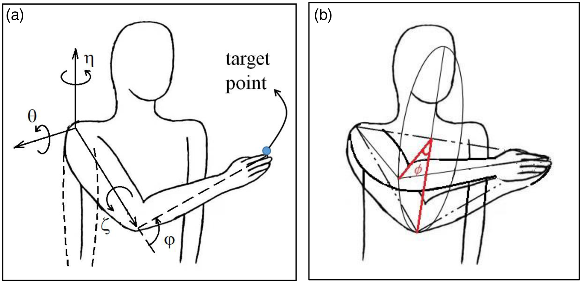
Figure 1. Inverse kinematic problem and analytical inverse kinematic method: (a) Inverse kinematic problem. (Dashed line shows the initial position of the arm. η, θ, ζ, ϕ are the joint angles, which are the shoulder adduction, shoulder flexion, shoulder rotation and elbow flexion, respectively.) (b) Definition of swivel angle.
The swivel angle is defined around the middle rotation axis (an axis pointing from shoulder joint center to wrist joint center), which can be determined by applying joint limits [Reference Kallmann18, Reference Molla and Boulic19]. However, joint limits can only provide a possible range of angles, instead of a specific swivel angle [Reference Aristidou, Lasenby, Chrysanthou and Shamir10]. Tolani et al pointed out three ways of selecting an appropriate swivel angle, from the possible range of angles: (1) select the midpoint of the possible range; (2) choose a possible value which is closest to a desired value; and (3) find a swivel angle value of φ which minimizes an arbitrary objective function [Reference Tolani, Goswami and Badler15]. This research focuses on the third approach, combining objective functions with the analytic IK method, in order to find an accurate solution, as well as to explore the mechanisms of the body posture determination.
1.2. Body oosture optimization and cost function
In this paper, body posture optimization (BPO) is combined into a previous AIK method in order to achieve a scientific determination of the swivel angle. Previous BOP problem is defined as follows. Previous researchers try to find the configuration (joint angles q) of a human body when the fingertip or other end-effector reaches the target point [Reference Yang, Marler and Rahmatalla2]. The hypothesis is that human performance measures govern the movements of human bodies. Based on this hypothesis, the BPO problem can be formulated as follows [Reference Yang, Marler and Rahmatalla2, Reference Mi, Yang and Abdel-Malek20, Reference Marler, Rahmatalla, Shanahan and Abdel-Malek21]:
Find: q ∈ R DOF
to minimize: f obj ( q )
subject to: distance = ||
x
end-effector
(
q
) –
x
target-point
|| < ${\unicode[Times]{x025B}}$
q i L < q i < q i U (i = 1, 2, …, DOF)
where fobj is an arbitrary objective function;
q is the joint angle vector, whose elements are joint vectors;
R indicates the real number space; ${\unicode[Times]{x025B}}$
is a small number close to zero;
${\unicode[Times]{x025B}}$
is a small number close to zero;
x end-effector (q) is the position vector of the end-effector, as a function of the joint angles;
x target-point is the position vector of the target point;
DOF is the total number of the degree-of-freedom of the applied kinematic structure.
qi is the ith element of the joint angle vector q, which is equal to the ith joint angle of the kinematic structure;
qi L and qi U are the lower and upper limits of the ith joint angle, respectively.
It is shown that the objective function is an important part of the BPO problem. Cost functions are functions evaluating human performance measures [Reference Mi, Yang and Abdel-Malek20], which can be applied as the objective functions, for the determination of human body posture. One thing that the authors wish to point out here is that this paper combines AIK with the BPO method, where the joint limit model of AIK performs as the constraint (details are discussed in the methodology section). Therefore, this section discusses different objective functions without considering the complete constrained optimization problem.
In order to determine which cost function(s) to be applied in this research, a literature review has been conducted (shown in Table I). Thirteen publications are studied in this review (Table I). Since one of the aims of this research is studying the mechanism of body-posture prediction, only those publications, related to human postures, are studied, while publications on robotics are excluded.
Table I. Selected studies and applied cost functions.

Among selected publications, the joint discomfort function is the most commonly applied cost function. The joint displacement function and delta potential energy function are the second most commonly applied cost functions. Therefore, the joint discomfort function, joint displacement function and delta potential energy function are analyzed in this research.
Based on searched literature, previous objective functions can be categorized into single objective functions and multiple objective functions. (In this section, bi-criterion objective functions are also categorized as multiple objective functions.) Multiple objective functions can also be categorized into two types: one is the product of different cost functions [Reference Rout, Tripathy, Dash and Dhupal22], while the other is weighted sum of different cost functions [Reference Marler, Arora, Yang, Kim and Abdel-Malek1, Reference Yang, Marler and Rahmatalla2, Reference Azizi, Dadarkhah and Asgharpour Masouleh8]. It has been reported that the combination of different cost functions (i.e., multiple objective functions [Reference Kashi, Avrahami, Rosen and Brand23]) is able to increase the accuracy of predicted body postures [Reference Admiraal, Kusters and Gielen16]. However, based on searched literature, there is not a systematic approach to accurately determine the weights of different cost functions [Reference Xie and Zhao24]. In addition, previous research has not clarified how the different cost functions coupled together are.
1.2.1. Delta potential energy
Delta potential energy describes the change of the gravity potential energy of human body, from initial posture to final posture [Reference Mi, Yang and Abdel-Malek20]. Eq. (1) shows a commonly applied formulation of the delta potential energy function [Reference Mi, Yang and Abdel-Malek20].
 \begin{equation}f_{dpe}\left({\boldsymbol{q}}\right)=\sum _{i=1}^{n}({m_{i}}\cdot g)^{2}\cdot (\Delta {h_{i}})^{2}\end{equation}
where m i is the mass of the i th body segment (Usually, a unit of kilogram is applied. In this research, m i is normalized by the body mass. Therefore, body mass is applied as the unit.),
g is the gravitational acceleration (The body mass multiplied by the gravitational acceleration is body weight. Therefore, the body weight (BW) is applied as the unit of mig.),
Δhi is the change of the height, of the centre of mass of the ith body segment, from the initial body posture to the final body posture (unit: meter or millimeter; millimeter is applied in this research).
For each couple of initial target point and final target point, as the swivel angle increases, Δhi will also increase, so that the delta potential energy of human arm will keep increasing. Therefore, the pure minimization of delta potential energy will always lead to the smallest swivel angle, which is probably not an accurate optimization.
1.2.2. Joint discomfort
The joint discomfort function has been widely applied to predict body posture [Reference Mi, Yang and Abdel-Malek20, Reference Rout, Tripathy, Dash and Dhupal22, Reference Jung, Choe and Kim25], which evaluates the musculoskeletal discomfort of human body [Reference Marler, Arora, Yang, Kim and Abdel-Malek1]. Based on searched literature, the latest joint discomfort function is developed by Marler et al. [Reference Marler, Rahmatalla, Shanahan and Abdel-Malek21], as shown in Eq. (2).
 \begin{equation}f_{discomf}({\boldsymbol{q}})=\frac{1}{G}\sum _{i=1}^{n}[\gamma _{i}\cdot (\Delta q_{i}^{n,norm})^2+G\cdot QU_{i}+G\cdot QL_{i}]\end{equation}
 \begin{equation}\Delta q_{i}^{n,norm}=\frac{q_{i}-q_{i}^{n}}{q_{i}^{u}-q_{i}^{L}}\end{equation}
 \begin{equation}QU_{i}=\left(0.5\cdot sin\left(\frac{5.0(q_{i}^{U}-{q_{i}})}{q_{i}^{U}-q_{i}^{L}}+1.571\right)+1\right)^{100}\end{equation}
 \begin{equation}QL_{i}=\left(0.5\cdot sin\left(\frac{5.0(q_{i}^{U}-{q_{i}})}{q_{i}^{U}-q_{i}^{L}}+1.571\right)+1\right)^{100}\end{equation}
where, q i is the value of i th joint angle (unit: degree or rad),
q i n is the neutral value of i th joint angle (unit: degree or rad),
q i U is the upper limit of the i th joint angle (unit: degree or rad),
q i L is the lower limit of the i th joint angle (unit: degree or rad), $\Delta {q}_{\text{i}}^{\text{i},\text{norm}}$
is the normalized value of the ith joint angle, based on the neutral joint angle value (as shown in Eq. (3)). Therefore, it has no unit.
$\Delta {q}_{\text{i}}^{\text{i},\text{norm}}$
is the normalized value of the ith joint angle, based on the neutral joint angle value (as shown in Eq. (3)). Therefore, it has no unit.
γ i is the joint weight (without unit),
QUi is the joint limit term expressed in Eq. (4),
QLi is the joint limit term expressed in Eq. (5),
G is a magnifying ratio (G > 1) for the joint limit terms QUi and QLi. The function in Eq. (2) is divided by G, in order to prevent the joint discomfort function from having extremely high values, when compared with the other cost functions [Reference Marler, Arora, Yang, Kim and Abdel-Malek1].
For each joint, they evaluate its discomfort by two facts: (a) joint discomfort decreases when a segment gets close to its neutral position; (b) joint discomfort rapidly increases when a segment gets close to its limits [Reference Marler, Arora, Yang, Kim and Abdel-Malek1]. Based on searched literature, its performance has not been evaluated by experiment data. Therefore, in this research, the performance of the joint discomfort function is evaluated by extracted experiment data, before being combined with another cost function.
1.2.3. Joint displacement
The joint displacement evaluates the angular displacement of each joint. In some research, the joint displacement is calculated from the neutral position [Reference Marler, Arora, Yang, Kim and Abdel-Malek1, Reference Mi, Yang and Abdel-Malek20], while, in other research, it is calculated from the initial position (i.e., the starting posture of the current analyzed motion or the end posture of a previous motion if a continuous motion is analyzed) [Reference Kashi, Avrahami, Rosen and Brand23]. When calculated from the initial position, the joint displacement is proportional to the energy expenditure of the motion from initial posture to final posture [Reference Kashi, Avrahami, Rosen and Brand23], which estimates the effect of the initial posture to the final posture. Therefore, in this research, joint displacement is calculated from initial posture. A commonly used formulation of the joint displacement function is shown in Eq. (6) [Reference Zou, Zhang, (James) and Gragg26].
 \begin{align} f_{displace}\left({\boldsymbol{q}}\right)=\sum _{i=1}^{n}\omega _{i}\cdot (\Delta q_{i}^{i,norm})^{2}\end{align}
 \begin{align} \Delta q_{i}^{i,norm}=\frac{q_{i}-q_{i}^{i}}{q_{i}^{u}-q_{i}^{L}} \end{align}
where q i i is the initial value of i th joint angle (unit: degree or rad),
ω i is the joint weight of the i th joint angle (with no unit). $\Delta \text{q}_{\text{i}}^{\text{i},\text{norm}}$
is the normalized value of the ith joint angle, based on the initial joint angle value (shown in Eq. (7) [Reference Marler, Arora, Yang, Kim and Abdel-Malek1]). Therefore, it has no unit.
$\Delta \text{q}_{\text{i}}^{\text{i},\text{norm}}$
is the normalized value of the ith joint angle, based on the initial joint angle value (shown in Eq. (7) [Reference Marler, Arora, Yang, Kim and Abdel-Malek1]). Therefore, it has no unit.
Zou et al. determined the weights in joint displacement function by means of inverse optimization [Reference Zou, Zhang, (James) and Gragg26]. Their joint displacement function is validated in whole-body reaching tasks and predicts reasonably accurate body postures [Reference Zou, Zhang, (James) and Gragg26]. However, when the torso is fixed, the accuracy of the determined joint angle values turns out to be low, which exhibits that the joint displacement function is not feasible for all types of reaching tasks. Further analysis needs to be conducted on its performance.
Therefore, in this research, we focus on the reaching tasks without motion of torso. Selected single objective functions (the joint displacement function and joint discomfort function) were initially combined with AIK method, respectively. Then, we examined the accuracy of the body postures, predicted by the joint displacement function [Reference Zou, Zhang, (James) and Gragg26] and the joint discomfort function [Reference Marler, Rahmatalla, Shanahan and Abdel-Malek21]. Then, we comprehensively combined the selected single objective functions together, proposing a new bi-criterion objective function. We have also validated the accuracy of this proposed bi-criterion objective function and studied the effect of the weight of joint discomfort, on the accuracy of predicted joint angle.
2. Kinematic model
In order to combine the AIK method with an optimization model (i.e., adding objective functions to the AIK method), a rigid-segmental model of the right upper limb of human beings is established in MATLAB, according to the body segment parameters exhibited in a publication of Dumas et al. [Reference Dumas, Chèze and Verriest27]. A human body model should consist of a kinematic structure and motion equations. In this paper, the established kinematic structure is made up with segmental vectors (vectors which represent the length and orientation of each segment) (Fig. 2(a)), where each vector represents a body segment. Once the position of the right shoulder joint centre (X 6 ) is given, the positions of the right elbow joint centre (X 7 ) and right second fingertip (X 8 ) can be calculated as Eq. (8).

Figure 2. The kinematic structure applied in this paper: (a) anatomical meaning of involved segmental vectors and anatomical nodes; (b) Kinematic structure of the established human body model, as well as the involved joint angle notations.
 \begin{align} {\boldsymbol{X}}_{{\boldsymbol{i}}}={\boldsymbol{X}}_{\textbf{6}}+\sum\nolimits_{j=6}^{i-1}{\boldsymbol{V}}_{{\boldsymbol{j}}}\quad (i=7,8)\end{align}
Segmental vectors are motivated by joint angles. In this model, each joint has an index as illustrated in Fig. 2(a). For example, the joint index for the right shoulder joint is 6 (Fig. 2(b)). For an arbitrary joint with a joint index i, joint angles are defined by global-frame-based ZYZ sequence. To be specific, the rotation of each joint is divided into three rotations. In the first rotation, an angle αi, 4 is performed around the z-axis, where i is the joint index. In the second rotation, an angle αi, 2 is performed around the y-axis of the global coordinate system. Finally, in the third rotation, an angle αi, 3 is performed around the z-axis of the global coordinate system again. Thus, the rotation matrix of an arbitrary joint i (R i ) can be deduced as Eq. (9a), which is equivalent to Euler’s ZYZ sequence.
 \begin{align} {\boldsymbol{R}}_{{\boldsymbol{j}}}={\boldsymbol{R}}_{{\boldsymbol{z}}}(\alpha_{i,3})\cdot{\boldsymbol{R}}_{{\boldsymbol{y}}}(\alpha_{i,2})\cdot{\boldsymbol{R}}_{{\boldsymbol{z}}}(\alpha_{i,4})\end{align}
where R y and R z represent basic rotation matrices, around y and z axes, respectively.
The basic rotation matrices around y and z axes, with an arbitrary rotational angle α, R y (α) and R z (α), can be calculated as Eqs. (9b) and (9c).
 \begin{equation}{\boldsymbol{R}}_y (\alpha) = \left(\begin{array}{c@{\quad}c@{\quad}c} \cos \alpha & {}0 & {}\sin \alpha \\ 0 {}& 1 & {}0\\ -\sin \alpha {}& 0 & {}\cos \alpha \end{array}\right)\end{equation}
 \begin{equation}{\boldsymbol{R}}_z (\alpha) =\left(\begin{array}{c@{\quad}c@{\quad}c} \cos \alpha & {}-\sin \alpha & {}0\\ \sin \alpha & {}\cos \alpha & {}0\\ 0 & {}0 & {}1 \end{array}\right)\end{equation}
Based on this adjusted notation for joint angles, an adjustment has been made to the storage of the joint angles. In previous research, all the joint angles are stored as a vector, which can make it difficult for users to match the index of a joint angle with its anatomical meaning. As Fig 2(d) shows, in this research, all the joint angles are stored in a matrix, where the first index is the joint notation, and the second index is the axis notation. In order to make the index easy to remember, the axis indices 1, 2, and 3 are matched with the x, y, and z axes of the global coordinate system, respectively.
Since there are two rotational angles around the z axis, the first rotational angle αι,4 is stored in the fourth column. In this way, for the upper limb posture determination, which is discussed in this paper, α6,2, α6,3, α6,4, and α7,2 are right shoulder flexion/extension, right shoulder abduction/adduction, right shoulder rotation and right elbow flexion/extension. If the right clavicle (V 5 ) is set as the reference, then the orientations of right upper arm (V 6 ) and right forearm (V 7 ) can be calculated as Eqs. (10a) and (10b).
 \begin{equation}{\boldsymbol{V\!}}_{{\boldsymbol{6}}}={\boldsymbol{R}}_{{\boldsymbol{6}}}\, {\boldsymbol{V\!}}_{{\boldsymbol{6}}}{}^{\textbf{(0)}}\end{equation}
 \begin{equation}{\boldsymbol{V\!}}_{{\boldsymbol{7}}} = {\boldsymbol{R}}_{{\boldsymbol{6}}}\, {\boldsymbol{R}}_{{\boldsymbol{7}}}\,{\boldsymbol{V\!}}_{{\boldsymbol{7}}}{}^{\textbf{(0)}}\end{equation}
where V 6 (0) and V 7 (0) are initial orientations of right upper arm and right forearm, in the neutral standing posture, respectively. (For the right elbow (X 7 ), α7, 3 = α7, 4 = 0. If we substitute this into Eq. (9c), we can get the result that R z (α7, 3) = R z (α7, 4) = I (In this paper, I represents the identity matrix.) Therefore, by means of substituting this result into Eq. (9a), R 7 = R y (α7, 2).)
Then, by means of substituting Eqs. (10a) and (10b) into Eq. (8c), the positions of the right elbow (X 7 ) and right fingertip (X 8 ) can be calculated as Eqs. (11a) and (11b), which is equivalent to the conventions established by Denavit and Hartenberg [Reference Denavit and Hartenberg13].
 \begin{equation}{\boldsymbol{X}}_{{\boldsymbol{7}}} = {\boldsymbol{X}}_{{\boldsymbol{6}}} + {\boldsymbol{R}}_{{\boldsymbol{6}}}\, {\boldsymbol{V}}_{{\boldsymbol{6}}}{}^{\textbf{(0)}}\end{equation}
 \begin{equation}{\boldsymbol{X}}_{{\boldsymbol{8}}} = {\boldsymbol{X}}_{{\boldsymbol{6}}} + {\boldsymbol{R}}_{{\boldsymbol{6}}}\, {\boldsymbol{V}}_{{\boldsymbol{6}}}{}^{\textbf{(0)}} + {\boldsymbol{R}}_{{\boldsymbol{6}}}\,{\boldsymbol{R}}_{{\boldsymbol{7}}}\, {\boldsymbol{V}}_{{\boldsymbol{7}}}{}^{\textbf{(0)}}\end{equation}
3. Methodology
This section introduces how we combine the AIK method with body posture optimization, analyze present objective functions, and develop a bi-criterion objective function. The combination between AIK method and body posture optimization is an important target of this research, which is expected to combine the solving efficiency of AIK methods with the accuracy of body posture optimization. The other target of this research is to develop an objective function with comprehensive physical meaning, attempting to have a deeper view on the mechanism of the determination of human body posture.
3.1. Analytic inverse kinematic method
Molla and Boulic proposed a singularity-free AIK method, named as Middle Rotation Axis (MRA), which can be formalized into three steps: (i) Determine the elbow flexion; (ii) Bring the end-joint (wrist) to the target position; (iii) Determine the mid-joint (elbow) position by satisfying the shoulder joint limit and wrist joint limit [Reference Molla and Boulic19].
In this research, as shown in Fig. 3, the MRA-AIK method is achieved by four steps. The first step solves the elbow flexion angle, as illustrated by Tolani et al. [Reference Tolani, Goswami and Badler15]. Once the target point position is given, then the value of the elbow flexion angle will be purely dependent on the distance between the shoulder joint center and the target point [Reference Tolani, Goswami and Badler15]. Similar with previous research [Reference Tolani, Goswami and Badler15, Reference Kallmann18, Reference Molla and Boulic19], in this paper, Cosine Law is applied to calculate the elbow flexion angle (α7, 2), as described in Eq. (12a) (in Fig. 4).

Figure 3. Workflow of the developed method (The notation S, E and H notes the shoulder joint centre, elbow joint centre and the third finger tip of right hand, respectively, while T represents the position of the target point.).

Figure 4. Equation and schematics of the first three steps.
Next, the shoulder abduction/adduction angle (α6, 3) is solved in step 2, according to Eq. (12.2) (in Fig. 4), where x6 and y6 are the x and y coordinates of the shoulder joint position X 6 , respectively; while xt and yt are the x and y coordinates of the target point position T. After this step, the upper arm, the lower arm, and the target point will be moved into the same plane.
The shoulder flexion angle (α6, 2) is solved in step 3, according to Eq. (12.3) (in Fig. 4), where d t ’ and d t are vectors pointing from the right shoulder joint centre (X 6 ) to the 2nd right fingertip (X 8 ) (determined in step 2) and the target point position T, respectively. This step moves the fingertip to the target point.
The swivel angle φ is activated in the 4th step), in order to calculate the rotation matrix of the entire upper limb in the 4th step. A function RERT (e, φ) is define in Eq. (12.6) (shown in Fig. 5), according to Euler’s Rotation Theorem [Reference Olguín Díaz28]. In Eq. (12.6), “I” represents the identity matrix. [e]* represents an operation, which transfer an arbitrary unit vector e to a matrix [e]*, as expressed in Eq (12.7) (shown in Fig. 5). The prime symbol (’) represents transfer matrix.

Figure 5. Schematic, pseudocode and equations of the fourth step.
When the swivel angle φ increases from 0 to φlim degree (φlim represents the upper limit value of the swivel angle φ; as shown in the pseudocode in Fig. 6), the shoulder flexion angle (α6, 2) and shoulder abduction angle (α6, 3) are calculated by Eqs. (12.8) and (12.9) (shown in Fig. 5), respectively. Then, the shoulder rotation angle α6, 4 (marked as τ in the pseudocode) increases from 0 to τlim degree, until the 2nd right fingertip reaches the target position. The criterion is set as that y8 must be larger than yt (when the 2nd right fingertip crosses the target point, from the right to the left).

Figure 6. Definition of the swing angles of the shoulder joint (X, Y and Z (on the right bottom) indicate the coordinates of the global coordinate system, while Xj, Yj and Zj indicate the coordinates of the shoulder joint coordinate system for the shoulder joint limit model) (refs. [31, Reference Engin and Chen30]).
Eventually, for each value of the swivel angle φ, the value of the objective function fobj will be calculated by substituting the determined set of joint positions (X) and joint angles (α) (as shown in the pseudocode of Fig. 5).
3.2. Body posture optimization (BPO)
3.2.1. Variable and constraints
An improved upper limb posture determination method is then developed by merging body posture optimization into the third step of MAR-AIK method (noted as “step 4” in Fig. 3, since the second step of the AIK method is divided into two sub-steps). Based on MAR, the optimization variable for reaching tasks is deduced from a set of joint angles (shoulder adduction, shoulder flexion, shoulder rotation and elbow extension) to only one variable, the swivel angle $\phi$
.
$\phi$
.
Two constraints are applied in this optimization problem. The first one is the shoulder joint limit. In this research, the shoulder joint limit model proposed by Grassia [Reference Grassia29] is applied. Grassia proposed an exponent map (swing and twist angles) as shown in Fig. 6, where the z axis points the neutral direction of the range of shoulder joint limit [Reference Grassia29]. In this research, the neutral direction is determined based on the parameters provided by Engin and Chen [Reference Engin and Chen30]. The x axis is inside a vertical plane and perpendicular to the z axis, while the y axis is perpendicular to both the x axis and y axis [Reference Grassia29].
To be specific, if we mark the three element-vectors, in the x, y, and z directions of the shoulder joint coordinate system, as e sx , e sy, and e sz , respectively; then, esx = (0, 0, 1)T, esy = (0, -1, 0)T, esz = (1, 0, 0)T (here “T” represent the transferring operation for matrices). Then, if we mark the three element-vectors, in the x, y and z directions of the joint limit coordinate system, as e jx , e jy, and e jz , respectively; then the three axis directions of the joint limit coordinate system (XjYjZj, shown in Fig. 6) can be calculated by Eqs. (13a), (13b), and (13c), where φn and θn are two orientation angles indicating the neutral direction of the shoulder joint (Zj), defined by Engin and Chen [Reference Engin and Chen30], with values of 59 degree and 21 degrees, respectively.
 \begin{equation}{\boldsymbol{e}}_{\textbf{jx}}={\boldsymbol{R}}_{\textbf{z}}(-\phi_{\rm n})\;\;{\boldsymbol{R}}_{{\boldsymbol{y}}}(\theta_n)\;\;{\boldsymbol{e}}_{\textbf{sx}}\end{equation}
 \begin{equation}{\boldsymbol{e}}_{\textbf{jy}}={\boldsymbol{R}}_{\textbf{z}}(-\phi_{\rm n})\;\;{\boldsymbol{R}}_{{\boldsymbol{y}}}(\theta_n)\;\;{\boldsymbol{e}}_{\textbf{sy}}\end{equation}
 \begin{equation}{\boldsymbol{e}}_{\textbf{jz}}={\boldsymbol{R}}_{\textbf{z}}(-\phi_{\rm n})\;\;{\boldsymbol{R}}_{{\boldsymbol{y}}}(\theta_n)\;\;{\boldsymbol{e}}_{\textbf{sz}}\end{equation}
The vector d is in the direction of the upper arm, with a scale equal to the swing angle value (The swing angle is defined as shown by the hollow arrow in Fig. 6. In this research, the unit of the shoulder swing is degree.) [Reference Grassia29]. Then the vector d is projected on the xj –yj plane (The origin o is the center of shoulder joint.). (To be specific, if we name the projective vector of vector d, on the coordinate direction Zj, as vector d z , and define the projective vector of vector d, on the xj –yj plane, as vector d xy , then d xy can be calculated as d xy = d – d z .) sx and sy are the two components of the projection, which are defined as two components of the shoulder swing angle. The shoulder twist (i.e., shoulder rotation) is then described as a rotation angle around the vector d. in this way, the shoulder joint limit is modelled as two parts: swing limit and twist limit. The swing limit proposed by Grassia is shown by Eq. (14). When the shoulder swing is inside its limit, the value of function f will be negative [Reference Grassia29].
 \begin{equation}f(s_x,s_y) = (s_x/r_x)^2+(s_y/r_y)^2 - 1 \end{equation}
rx and ry describe the maximum values of sx and sy. Typical values of rx and ry are 95 degree and 31 degrees, respectively [31]. However, in this research, it is found that, when ry = 31 degree, the possible range of shoulder rotation will not cover all the experimental values in [Reference Admiraal, Kusters and Gielen16]. Therefore, ry is increase to 60 degrees. The twist limit is modelled as the upper and lower limit of shoulder rotation [Reference Grassia29]. According to the publication of Marler et al. [Reference Marler, Arora, Yang, Kim and Abdel-Malek1], in this research, the upper and lower limit of shoulder rotation are set as 130 degree and 0 degree, respectively, where internal rotation is positive.
Another constraint is also added, which is that the swivel angle φ cannot go beyond 120 degrees. The reason for adding this constraint is that, based on the definition of the swivel angle (as shown in Fig. 2), a swivel angle larger than 120 degree is obviously unnatural. It is worth to point out that the distance constraint [Reference Marler, Arora, Yang, Kim and Abdel-Malek1], which requires the end-effector to reach the target point, is satisfied by the first two steps of the AIK method (from step 1 to step 3 of the Fig. 3, the second step of the AIK method is divided into two sub-steps in Fig. 3). Therefore, this constraint is no longer involved in the optimization problem.
3.2.2. Combination between MRA-AIK and BPO
As shown in Fig. 3, the optimization module is merged to the fourth step of the MRA-AIK method. In the fourth step, the swivel angle is increased from 0 to 120 degree, with a step of 1 degree. For each swivel angle value, it will be initially examined that whether the upper arm is inside the shoulder joint limit which was proposed by Grassia [Reference Grassia29]. If the upper arm is inside the shoulder limit, the objective function value will be calculated. (The inputs of this developed method are the target point position and initial upper limb posture. The initial upper limb posture data will be utilized when the objective function is the joint displacement function.)
The swivel angle value, corresponding to the minimum objective function value, will be output. Then, the joint angles will be re-calculated, based on the value of the swivel angle. These re-calculated upper limb joint angle values will enable the calculation of the positions of upper limb joint centers will be calculated, and the construction and plotting of the determined upper limb postures.
3.3. Simulation of previous objective functions
The feasibilities of applying the joint displacement function and joint discomfort function as the objective function are primarily judged, with the experimental results of Admiraal et al. [Reference Admiraal, Kusters and Gielen16], whose extracted data has also been utilized by Kashi et al. [Reference Kashi, Avrahami, Rosen and Brand23]. Nine subjects are involved in the experiment of Admiraal et al. while five target points are set up, thus twenty couples of initial and final target points are studied.
Admiraal et al quantified human arm postures by the rotational angle of shoulder. In this simulation, measured shoulder rotation values are plotted, versus those shoulder rotation values, predicted by applying the joint discomfort function and joint displacement function, respectively. In each plot, a straight blue line, with a slope equal to one, is plotted, which indicates “measured value = predicted value.”
Joint weights of joint displacement function are cited from the publication of Zou et al. [Reference Zou, Zhang, (James) and Gragg26], while the joint discomfort function is cited from the publication of Marler et al. [Reference Marler, Rahmatalla, Shanahan and Abdel-Malek21]. The delta potential energy function is not involved since it will always lead to the smallest swivel angle value.
3.4. Proposed bi-criterion objective function
Further simulation was conducted on the joint discomfort function, joint displacement function, and delta potential energy function, for the five target points selected in the experiment of Admiraal et al. [Reference Admiraal, Kusters and Gielen16]. Since joint discomfort curves are “well-shaped” (changes rapidly on the “wall” of these “well”, but slightly on the “bottom” of these “well”, as shown in Section 4), a bi-criterion objective function (f discomf-displace ) has been proposed by adding joint discomfort and joint displacement together (shown in (15)), where α is a coefficient.
 \begin{equation}f_{discomf-displace} = \alpha\cdot f_{discomf} + f_{displace}\end{equation}
Then, on the “wall” of these “well,” the value of this new objective function will be dependent on joint discomfort, while, on the bottom of these “well,” the value of this new objective function will be mainly determined by joint displacement. Therefore, by means of this, the predicted shoulder rotation value, for each couple of initial target point and final target point, will be limited into a relatively small range, and become more accurate.
3.5 Linear regression and suboptimal coefficient value
For an ideal IK method, for each couple of initial target point and final target point, the determined shoulder rotation value (ζpredicted) should be equal to the measured shoulder rotation value (ζmeasured) (i.e., ζpredicted = ζmeasured), which is a linear relation. Therefore, linear regression is applied to estimate the accuracy of the shoulder rotation values, determined by the developed AIK method. Shoulder rotation value residuals (ζresidual) are calculated as the difference between the measured values (ζmeasured) and linear regression values (ζregression) (shown in Eq. (16)). A residual analysis is then conducted by plotting the average residual values, among the 9 subjects, involved in the experiment of Admiraal et al. [Reference Admiraal, Kusters and Gielen16], in order to compare the performance of the bi-criterion objective function and joint discomfort function, based on the developed AIK method. Coefficient of determination (R2) (shown in Eq. (10b) [Reference Steel and Torrie32]) is also calculated to quantify the accuracy of the shoulder rotation values, determined by the developed AIK method.
 \begin{equation}\zeta_{residual} = \zeta_{measured} - \zeta_{regression}\end{equation}
where ζmeasured is the measured value (unit: degree).
ζregression is the linear regression value (unit: degree).
 \begin{equation}R^{2}=1-\frac{RSS}{TSS}\end{equation}
where RSS is the sum of squares of residuals (ζresidual);
TSS is the total sum of the squares of linear regression values (ζregression).
In Eq. (15), if α keeps increasing, then f discomf-displace will eventually become equivalent to f discomf . On the contrary, if α becomes zero, then f discomf-displace will become f displace . Based on the research of Admiraal et al, body postures are determined by the final target point position and the initial body posture together [Reference Admiraal, Kusters and Gielen16]. However, the minimization of the joint discomfort function does not reflect the effect of the initial body posture. Therefore, theoretically, when α keeps increasing, the accuracy of predicted shoulder rotation values will not keep increasing but start decreasing at a certain point. In this way, R2 can be regarded as a function of coefficient α, as shown in Eq. (18), whose domain is from zero to positive infinite. Furthermore, theoretically, a suboptimal value of α (αopt) exists between zero and infinite.
 \begin{equation}R^2 = R^2 (\alpha)\end{equation}
A pilot search is initially conducted. The starting value of α is set to be 10−14, by the best guess. Then the coefficient value is magnified/divided by 100, and α values of 10−16 and 10−12 are attempted. A step of 4 is set for the power number of α. Then a golden section search [Reference Kiefer33] is applied in the interval (0.0001, 10,000), to find out the suboptimal coefficient value (αopt).
4. Results and discussion
This section shows the comparison between the shoulder rotation values, determined by the joint discomfort function, joint displacement function, and proposed bi-criterion objective function, respectively, and the shoulder rotation values measured by Admiraal et al. [Reference Admiraal, Kusters and Gielen16]. The simulation result of the joint discomfort function, joint displacement function, and delta potential energy function is also shown in this section.
4.1. Simulation on previous cost functions
Figure 7 shows the value of joint discomfort, joint displacement, and delta potential energy, changing with the swivel angle, within joint limit, which provides further accordance for the combination of the joint discomfort function and joint displacement function (as discussed in Section 3.3). The five target points are cited from the publication of Admiraal et al. [Reference Admiraal, Kusters and Gielen16]. For the joint displacement function and delta potential energy function, the initial posture in this simulation is neutral standing.

Figure 7. Change of joint displacement, joint discomfort and delta potential energy versus swivel angle, within joint limit.
As shown in Fig. 7, joint discomfort curves are “well-shaped.” Therefore, by adding the joint discomfort function to the joint displacement function, the predicted shoulder rotation value is expected to be limited in a more accurate range.
4.2. Proposed bi-criterion objective function
Figure 8 plots the measured shoulder rotation values [Reference Admiraal, Kusters and Gielen16] versus the shoulder rotation values, determined by applying proposed objective function with different coefficient values. The measured shoulder rotation angle values, used as the vertical coordinate of each subfigure in Fig. 8, were extracted from a previous publication of Admiraal et al. [Reference Admiraal, Kusters and Gielen16]. The same data group (measured shoulder rotation angle values) is also used in Fig. 9.

Figure 8. Extracted shoulder rotation values [Reference Admiraal, Kusters and Gielen16] versus the shoulder rotation values, predicted by proposed bi-criterion objective function, for different coefficient values.

Figure 9. Measured shoulder rotation values (ζmeasured), versus the determined values (ζpredicted). (a)”Previous AIK method 1” (selecting the smallest swivel angle value within the shoulder joint limit); (b)”Previous AIK method 2” (selecting the middle swivel angle value within the shoulder joint limit); (c) the developed AIK method with the joint discomfort function; (d) the developed AIK method with the proposed bi-criterion objective function and the suboptimal coefficient value (when the coefficient (α) equals to 7.7).
Figure 8(a) shows the performance of the joint displacement function. (The proposed bi-criterion objective function is equal to the joint displacement function when the coefficient value is zero.) As shown in Fig. 8(a), the majority of the data points spread in a triangular area, which shows that there is no obvious relation between the predicted shoulder rotation values and measured values. This result is different from the result of Zou et al. In the research of Zou et al., the joint displacement function predicts reasonable body postures [Reference Zou, Zhang, (James) and Gragg26]. This phenomenon indicates that an IK method, validated by whole-body reaching motion, is possible to be inaccurate when the torso is fixed.
It is shown that, as the value of the coefficient of the joint discomfort function increases, data points gradually gathered into several columns. This phenomenon is caused by the fact that the joint discomfort function does not consider the effect of the initial posture, while the joint displacement function considers it. When the effect of the initial posture is neglected, the measured shoulder rotation values, with different starting target points, will be matched with the same predicted value. Therefore, when the coefficient of the joint discomfort function increases, data points with the same final target point will become closer and closer.
It is also exhibited that, generally, data points get more and more close to the straight blue line, whose slope is one. This blue line indicates the position where the measured value is equal to the predicted value. Therefore, this phenomenon shows that, by adding the joint discomfort function to the joint displacement function, the accuracy is increased indeed.
4.3. Suboptimal coefficient value
Figure 10 shows the accuracy of the predicted shoulder rotation values (evaluated by the coefficient of determination), changing by the value of α. As discussed in Section 3.6, the search of the optimal value of α consists of two phases – pilot search and golden section search. Figure 10(a) shows the result of the pilot search. As shown in Fig. 10(a), when the value of α increased from 10–16 to 104, the R2 value increases first, and then starts decreasing, which agrees with our hypothesis in Section 3, and also limits the optimal value of α into the range between 0.0001 and 10,000. Figure 10(b) shows the result of the golden section search. Based on the golden section search, the optimal α value for the subject 1, 6, 7, 8, and 9 is 13; the optimal α value for the subject 2 is 3; while the optimal value of α, for the subject 3, 4, and 5, is 1. Therefore, the global optimal value of α is determined as the weighted average, which is 7.7.

Figure 10. The coefficient of determination values of all the nine subjects, changing with the value of α. (a) Result of the pilot search; (b) result of the golden section search.
4.4. Performance of the finalized function
This subsection exhibits the performance of the developed AIK method, as well as compares its performance with that of the previous AIK methods. Figure 9 plots the measured shoulder rotation values (ζmeasured) versus the values (ζpredicted), determined by different AIK methods. Subplots (a) and (b) show the results of previous AIK methods. “Previous AIK method 1” refers to the AIK method selecting the smallest swivel angle value, within the shoulder joint limit; while the “previous AIK method 2” refers to the AIK method selecting the middle swivel angle value, within the shoulder joint limit. (This notification of previous AIK methods also works in Table II and Fig. 11.) Subplots (c) and (d) show the results of the developed AIK method, with the joint discomfort function and proposed bi-criterion function (when the coefficient (α) equals to 7.7), respectively.
Table II. Coefficient of determination (R2) of the shoulder rotation values, determined by the previous AIK methods and the developed AIK method (with the proposed bi-criterion objective function (with optimal coefficient value (αopt)) and the joint discomfort function (fdiscomf), respectively).

* Selecting the smallest swivel angle value within the shoulder joint limit.
** Selecting the middle value of the swivel angle within the shoulder joint limit.
Table II compares the coefficient of determination (R2) values of the determined shoulder rotation values, determined by previous AIK methods and the developed AIK method, with the joint discomfort function and the proposed bi-criterion objective function. However, the coefficient of determination (R2) value cannot fully represent the relation that the determine shoulder rotation value (ζpredicted) should be equal to the measured shoulder rotation value (ζmeasured) (ζpredicted = ζmeasured) (e.g., the slope of the regression line is not considered.). Therefore, a residual analysis is conducted as an addition. Figure 11 shows the result of the residual analysis, which plots the absolute residual values (|ζresidual|). The red color indicates that the corresponding residual value is positive, while the blue color indicates that is negative.

Figure 11. Residual analysis for the previous AIK methods and the developed AIK method. (a)”Previous AIK method 1” (selecting the smallest swivel angle value within the shoulder joint limit); (b)”Previous AIK method 2” (selecting the middle swivel angle value within the shoulder joint limit); (c) the developed AIK method with the joint discomfort function; (d) the developed AIK method with the proposed bi-criterion objective function and the suboptimal coefficient value (when the coefficient (α) equals to 7.7).
4.4.1. Comparison between previous AIK methods
As shown in Fig. 9, the data points in Fig. 9(a) gather in three columns, which does not show a correlation between the measured shoulder rotation values and the shoulder rotation values determined by selecting the lowest swivel angle value, within the shoulder joint limit. On the contrary, the shoulder rotation values determined by the second previous AIK method (selecting the middle value of the swivel angle, within the shoulder joint limit) shows a rough correlation with the measured shoulder rotation values. (As shown in Fig. 9(b), the data points determined by “previous AIK method 2” gather in five columns, which roughly spread around the straight line with a slope of one.)
This difference between the performances of previous AIK methods is also quantified by the coefficient of determination (R2) value. As shown in Table II, the R2 value of the result of the “previous AIK method 2” (0.3528) is 228.7 percentage higher than that of the “previous AIK method 1” (0.0823). When it comes to the residual analysis, as shown in Fig. 11, the maximum residual of the “previous AIK method 2” (around 24 degrees, shown in Fig. 11(b)) is lower than that of the “previous AIK method 1” (around 27 degrees, shown in Fig. 11(a)), which also exhibits that accuracy of the “previous AIK method 2” is higher than the “previous AIK method 1.” Therefore, based on the comparison above, the “previous AIK method 2” (selecting the middle value of the swivel angle within the shoulder joint limit) is set as a standard to evaluate the performance of the developed AIK method (i.e., the developed AIK method is compared with the “previous AIK method 2” in Subsection 4.4.2.).
4.4.2. Comparison between the developed AIK method and previous AIK methods
Figure 9(a) and (b) exhibit the determined results of the developed AIK method, with the joint discomfort function and the proposed bi-criterion function, respectively. Compared with the “previous AIK method 2” (Fig. 9(b)), almost all the data points, determined by the developed AIK method, with both the joint discomfort function (Fig. 9(c)) and the proposed bi-criterion function (Fig. 9(d)) locate under the straight line with a slope of one. Moreover, the top of each column of data points, in Fig. 11(c) and (d), is either on or close to the straight line with a slope of one, which shows that the tendency of the determined result of the developed AIK method is very close to the relation that “ζpredicted = ζmeasured.”
This increase of the accuracy is also shown by the coefficient of determination (R2) (Table II). As shown in Table II, with the joint discomfort function, the developed AIK method determined shoulder rotation values with an R2 value of 0.8131, which is 130.5 percent higher that of the “previous AIK method 2” (0.3528). Moreover, the developed AIK method, with the proposed bi-criterion function (with the suboptimal coefficient value), determined shoulder rotation values with an R2 value of 0.8704, which is 146.7 percent higher than the “previous AIK method 2.” When it comes to the residual analysis, the maximum residual of the developed AIK method, with the joint discomfort function, is around 15 degree (shown in Fig. 11(c)); while the maximum residual with the proposed bi-criterion function is around 10 degree (shown in Fig. 11(a)). Compared with the “previous AIK method 2” (whose maximum residual is about 24 degree), the maximum residual values of the developed AIK method, with the joint discomfort function and the proposed bi-criterion function, decrease by approximately 37.5% and 58.3%, respectively. This result shows that, by means of combining the previous AIK method with a body posture optimization module, the accuracy of the MRA-AIK method, in the determination of upper limb postures, is obviously improved.
4.4.3. Comparison within the developed AIK method
As shown in Table II, for all the nine subjects, the proposed objective function with the suboptimal coefficient value (which is 7.7) determines more accurate shoulder rotation values. To be specific, the average coefficient of determination (R2) value, corresponding to the proposed objective function is 0.8704, increasing by 0.0573 (7%) from the R2 value corresponding to the joint discomfort function. It is also shown that, compared with the joint discomfort function, the proposed bi-criterion objective function decreases the inaccuracy of the prediction at final target 5. These two phenomena show that, by means of combining the joint discomfort function and the joint displacement function, as well as searching the suboptimal coefficient value for the proposed bi-criterion objective function, the performance of the developed AIK method is further improved.
It is also shown that, for the proposed bi-criterion objective function with the suboptimal coefficient value, data points spread into seven columns; while the data points determined with the joint discomfort function gather in 4 columns. This comparison also shows the advantage of the proposed bi-criterion objective function and the searched suboptimal coefficient value. However, since the proposed objective function involves the joint displacement function, it considers the effect of initial postures and should theoretically have 20 columns in the “measured value - predicted value” plot. Thus, the proposed objective function still has potential to be improved.
5. Summary and conclusions
This paper shows the development of an improved AIK method, based on the MRA (Middle Rotation Axis) AIK method and previous body-posture optimization methods. To summarize, this research has four major contributions as listed below.
-
1. This research combines the MRA-AIK method with body posture optimization, which increased the accuracy of the MRA-AIK method, in the determination of the human upper limb postures during tasks. By means of this combination, the shoulder joint limit model works as a constraint of the body posture optimization problem, which simplified the optimization procedure. Therefore, this combination is also expected to increase the computational efficiency, compared with previous body posture optimization methods.
-
2. Based on the developed AIK method, an innovative objective function is proposed by combining the joint discomfort function and the joint displacement function. We initially examined the performance of the joint displacement function. Although the joint displacement function predicts reasonable body postures for whole-body reaching tasks, result shows that it does not predict accurate body postures when the torso is fixed.
Based on the developed AIK method, the joint discomfort function predicts reasonable upper limb postures for reaching tasks. However, since it does not reflect the effects of the initial body postures, a bi-criterion objective function is proposed by adding the joint discomfort function and joint displacement function. Compared with previous bi-criterion and multiple objective functions, it is clear to see how the different components work together, in the proposed bi-criterion objective function, which makes our bi-criterion objective function mathematically comprehensive.
Results show that the accuracy of the proposed objective function is satisfactory and higher than both the joint discomfort function and joint displacement function, which not only convinces the performance of the developed AIK method (In the reaching tasks with the fingertip being the end-effector), but also adds to the reliability of the assumption that the natural human body posture is determined by minimizing both the discomfort and energy cost.
-
3. A systematic approach is applied to determine the coefficient value. This approach is also applicable for any other objective function with two components. In this approach, the coefficient of determination (R2) is selected to quantify the accuracy of the result of optimization. The determination of the suboptimal value of the coefficient (α) is based on previous published data. The larger data scale we have, the more accurate value of α will we determine. Golden section search is applied to determine the suboptimal value of the coefficient. The program can also be further improved, in order to automatically search for the optimal coefficient value.
-
4. In order to implement this developed AIK method, a simplified human body model is established in MATLAB, which provides users with higher flexibility. In this model, an adjusted data structure is applied for joint angles, which is more systematic and comprehensive than previous data structure. Although the developed AIK method is established on this human body model, the model itself is independent from the developed AIK method. Therefore, although the developed AIK method is so far only able to determine joint angles of the upper limb, a human body model is still established with all the body segments. Future research can continue to improve the developed AIK method and make it able to determine all the joint angles.
Limitations of the developed AIK method are described as follows.
Initially, although the combination between the MRA-AIK method and BPO is supposed to achieve higher computational efficiency, this hypothesis needs to be validated by further research. Secondly, for the determination of the suboptimal coefficient value (αopt), R2 cannot represent the relation that the determined values should be equal to the measured values. Therefore, other quantities should be applied to replace R2 in future research, such as the residual. Another limitation of the currently developed AIK method is that the movement of the wrist joint is omitted in the current stage of the developed AIK method. Therefore, the currently developed AIK method is not applicable in those cases when the hand orientation is constrained or limited (for example, when the hand orientation is affected by the geometry of the target or any barrier(s) in the working environment).
In addition, this research only focuses on the reaching task conducted by fingertips, when the torso fixed. Therefore, the suboptimal value of α, determined in this research, will probably change for other tasks. More research is supposed to be conducted on different tasks in the future. Moreover, since the upper limb strength depends on the upper limb posture, the weight of the load in hand can also impact the upper limb posture. In this paper, only the upper limb posture without a load in hand is discussed. The determination of the upper limb posture with load should be investigated in future research, while the suboptimal value of the coefficient is supposed to be impacted by the weight of the load.
Acknowledgment
This research is funded by the Natural Sciences and Engineering Research Council of Canada (NSERC) through Discovery Grant (RGPIN-2019-04585). The authors acknowledge that the experimental data, applied in this paper, is extracted from the publication of Admiraal et al [Reference Admiraal, Kusters and Gielen16].
Competing interests
The authors declare none.
Ethical considerations
None.
Author contributions
Jiahuan Chen conceived and designed the study (based on the PhD thesis of Dr. Xinming Li), finished programming, conducted data extraction, performed the analyses, and wrote the article.
Dr. Xinming Li applied for the funding which financially supported the study, and provided her comments and suggestions during discussions and by writing, especially on the data extraction method and paper formatting.
Jiahuan Chen and Dr. Xinming Li then revised this paper together, according to the nice comments and suggestions from the journal reviewers.


 Open access