


1. INTRODUCTION
Ocean current is neglected when computing the optimal speed in optimal ship routing. In previous papers (see Bijlsma (Reference Bijlsma2008), also for further references) we observed that ocean current could be included but that inclusion complicates things unnecessarily and does not contribute substantially to the final result. However, we did not indicate how the inclusion of ocean current could be performed. For the sake of completeness this omission is set right in this note. The reason is that the wind, which plays a similar role in aviation as ocean current in shipping (Bijlsma, Reference Bijlsma2009) in contrast to the effect of ocean current in optimal ship routing, is an important factor in optimal aircraft routing. Therefore it is convenient to have the disposal of a method, which can handle this kind of optimal problem.
2. INCLUSION OF THE OCEAN CURRENT IN OPTIMAL SHIP ROUTING
In order to simplify the computations the navigation area is mapped conformally onto a plane. Introducing a Cartesian coordinate system with coordinates x 1 and x 2 the equations of motion of the ship read:
where the dot denotes differentiation to the time t. The speed V and heading p are control variables, and S 1(t,x 1,x 2) and S 2(t,x 1,x 2) are the x 1 component and x 2 component of the ocean current. It is assumed that the nonzero fuel consumption per unit of time is described by the equation
where x 0 is the fuel consumption. The problem under consideration is to find continuous control functions V(t) and p(t) and a corresponding trajectory x(t)=(x 1(t),x 2(t)) satisfying the equations of motion (1) and (2), with initial and end conditions x i(0)=x i0,x i(t 1)=x i1(i=1,2), which minimize the integral:
The necessary condition for the control functions V(t) and p(t), and the trajectory x(t) to be optimal i.e. to give a solution of the optimal problem is that there exist continuously differentiable multipliers λ(t)=(λ0(t),λ1(t),λ2(t)), λ0(t)=constant⩽0 and a function H(t,x,V,p,λ)=λ0f 0+λ1(V cos p+S 1)+λ2(V sin p+S 2) so that the following conditions hold:
(a) The first necessary condition. On x(t) the Euler-Lagrange equations
 hold. Variables as subscripts denote partial differentiation.
(b) The necessary condition of Weierstrass. Along x(t) the inequality H(t,x(t),V,p,λ(t))⩽H(t,x(t),V(t),p(t),λ(t)) must hold for any t,0⩽t⩽t 1. In addition H(t 1,x(t 1),V(t 1),p(t 1),λ(t 1))=0.
It is supposed here that the arc x(t) is normal which implies the existence of a one-parameter family of arcs satisfying Equations (1) and (2) with the given initial and end conditions, and having x(t) as one of its members. As a consequence of normality the equality sign for the parameter λ0 is excluded. Solutions of the Euler-Lagrange equations with continuous control functions are called extremals. Observing that every part of an optimal trajectory is an optimal trajectory itself, which is a direct consequence of the principle of optimality (Bellman, Reference Bellman1957), the relation H=0 holds on x(t). We may write the Euler-Lagrange equations as:
We observe that the solution of the optimal problem does not change if λ1 and λ2 are multiplied by an arbitrary constant. This is the case because λ0 can be chosen arbitrarily and the multipliers λ0, λ1 and λ2 are defined up to a common factor of proportionality. Introducing polar coordinates, the initial values of the multipliers can be written as λ1(0)=cos a and λ2(0)=sin a for every choice of λ0. We choose λ0=−1. All extremals emanating from the starting point are found by varying the parameter a.
3. MODIFICATIONS IF OCEAN CURRENT IS INCLUDED
Using H=0, Equations (7) and (8) can be written as:
where V*=V+(λ1S 1+λ2S 2)/(λ1 cos p+λ2 sin p).
These equations express the necessary conditions so that the function:
of the variables V and p attains a maximum value along an extremal. The angle between (λ1, λ2) and (cos p, sin p) indicating the range of admissible values for p is acute and is assumed to be chosen to be sufficiently small throughout the region so that the speed V can satisfy the relations mentioned below. Application of a theorem on implicit functions (Hestenes, Reference Hestenes1966, p. 22) to H V=0 and H p=0 learns that the functions H V and H p and their partial derivatives to V and p must be continuous, and that the determinant ![]() must be different from zero in order that V and p are continuous functions. This condition also expresses that the equality sign in the Legendre condition, which is a direct consequence of the condition of Weierstrass, must be excluded. In that case the arc x(t) is called non-singular. Foregoing means in practice that there exist unique values of heading p and speed V along an extremal which maximize V*/f 0 (for V) as well as the projection of (cos p, sin p)V*/f 0 on (λ1, λ2) (for p). This is accomplished by maximizing (11).
must be different from zero in order that V and p are continuous functions. This condition also expresses that the equality sign in the Legendre condition, which is a direct consequence of the condition of Weierstrass, must be excluded. In that case the arc x(t) is called non-singular. Foregoing means in practice that there exist unique values of heading p and speed V along an extremal which maximize V*/f 0 (for V) as well as the projection of (cos p, sin p)V*/f 0 on (λ1, λ2) (for p). This is accomplished by maximizing (11).
The discussion that follows concerns solutions of Equations (1), (2), (5) and (6), which are continuous in their dependence on the parameter a. Application of a theorem on the initial value problem for a system of ordinary differential equations (Walter, Reference Walter1972, p. 93) gives the following result. Let the right-hand sides of Equations (1), (2), (5) and (6) be continuous for 0⩽t⩽t 1 and satisfy a Lipschitz condition with respect to x 1,x 2,λ1 and λ2. Then x i(t,a) and λi(t,a) (i=1,2; 0⩽t⩽t 1) as solutions of Equations (1), (2), (5) and (6) with x i(0)=x i0(i=1,2) are continuously differentiable with respect to t and continuous in their dependence on the parameter a defined by λ1(0)=cos a and λ2(0)=sin a.
This result makes it possible to introduce a numerical method for the solution of the optimal problem with the ocean current included. The continuous dependence of x 1,x 2,λ1 and λ2 on the parameter a is illustrated in Figure 1 showing a one-parameter family of extremals along which the sailing time is minimized. In this case the ocean current is not involved in the computation of the optimal ship's speed, which is the maximum speed. The optimal track from beginning to end point, which includes the ocean current, is obtained by selecting that extremal, which ends closest to the destination.
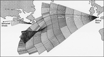
Figure 1. One-parameter family of extremals along which the sailing time is minimized, using wave information over the period 17 January-23 January 1970, fictitious ship's data and a 12-hours time step. The least-time track is indicated by the dashed line.
CONCLUSION
In this note it is indicated how ocean current could be included in the computation of the optimal speed in ship routing. Although the effect of ocean current in ship routing is generally negligible, inclusion of similar terms in other applications such as the wind in aircraft routing can be significant.

