


Introduction
The beginning of the melt season in snow-covered regions is an important stage in local and regional hydrology and climate. The surface albedo decreases as the snow changes from dry to wet, decreasing more dramatically when the seasonal snow cover is all melted, exposing bare ice on glaciers and soil and vegetation on non-glacierized areas. Meltwater moves rapidly through the snowpack and quickly affects stream discharge. We focus on frequent, regional-scale observations of glacier-snowpack properties in perennially snow- and glacier-covered areas of southeast Alaska, U.S.A., and along the Canadian border in order to observe snowmelt dynamics, a major part of glacier ablation. One factor that has a large effect on glacier mass balance is the length of the melt season (e.g. Reference KleinKlein, 1997). This paper uses new methods (first demonstrated in Reference Ramage and IsacksRamage and Isacks, 2002) to detect the beginning and end of the annual snowmelt season in mid-latitude regions. The focus of this paper is the regional view and interannual variations in the timing of snowmelt and runoff from 1988–98.
Snowmelt-detection algorithms are based on the fact that at a frequency > 10 GHz there is a large difference in brightness temperatures (T b) for dry vs wet snow (Reference Stiles and UlabyStiles and Ulaby, 1980; Reference Ulaby, Moore and FungUlaby and others, 1986). Numerous algorithms have been developed for determining the timing and extent of seasonal snowmelt on the Greenland and Antarctic ice sheets, for continental snow cover and for snow on sea ice (e.g. Reference HallHall and others, 1991; Reference Mote, Anderson, Kuivinen and RoweMote and others, 1993; Reference RidleyRidley, 1993; Reference Zwally and FieglesZwally and Fiegles, 1994; Reference Abdalati and SteffenAbdalati and Steffen, 1995, Reference Abdalati and Steffen1997; Reference AndersonAnderson, 1997; Reference Cavalieri, Parkinson, Gloersen, Comiso and ZwallyCavalieri and others, 1999). The techniques presented in this paper establish a new way of monitoring melt on perennially snow-covered areas that is sensitive to diurnal variability. Surface observations corroborate the interpretations of passive-microwave brightness temperatures on Juneau Icefield (Reference Ramage and IsacksRamage and Isacks, 2002). Some features of the seasonal passive-microwave signatures differ in other parts of southeast Alaska, such as the Saint Elias Mountains, but the differences follow logically from known differences in terrain characteristics, most notably altitude. Based on methods that successfully identify melt timing and character on Juneau Ice-field and the Saint Elias Mountains, this paper assesses melt dynamics on all perennially snow-covered regions in south-east Alaska and western British Columbia, Canada. Study of all the large southeast-Alaskan icefields makes it possible to estimate spatial and temporal variations of the snowmelt timing, duration and intensity. Changes in the timing of melt onset have implications for the timing and duration of both accumulation and ablation seasons on glaciers, thereby influencing a major component of glacier mass balance.
Data
Satellite data
Passive-microwave data come from three Defense Meteorological Satellite Program (DMSP) Special Sensor Microwave Imager (SSM/I) instruments (F08, F11, F13) that have a collective record extending back to August 1987. Data from January 1988–December 1998 are used in this paper (Table 1). Nominal SSM/I pixel resolution for the 37 GHz channels is 37 × 28 km2 (Reference Hollinger, Pierce and PoeHollinger and others, 1990). Data for this analysis have been regridded to the nominally 25 × 25 km2 Equal Area SSM/I Earth Grid (EASE-Grid) Northern Hemisphere projection and were provided by the U.S. National Snow and Ice Data Center, Boulder, Colorado. EASE-Grid data keep the ascending- and descending-orbit observations separate, a feature critical for calculating the diurnal T b range. Data for this region were rarely acquired on the descending orbit from February–November 1994. Melt detection depended on multiple daily observations, so there is a gap in our analysis for this period. T b distributions are similar for each sensor but cycle through a 2 hour range for each ∼2 week orbit cycle. The effect of the sensor on T b distribution is small (Reference Ramage and IsacksRamage and Isacks, 2002). All passive-microwave data in this paper are from the 37GHz vertically polarized SSM/I channel. The general technique also works for 19 GHz vertically and horizontally polarized channels and the 37 GHz horizontally polarized channel, but the 37 GHz vertically polarized channel is most sensitive to moisture variation and has the highest amplitude signal. Methods that combine channels (e.g. cross-polarized gradient ratio (XPGR), Reference Abdalati and SteffenAbdalati and Steffen, 1995, Reference Abdalati and Steffen1997) are very effective in polar regions, but give ambiguous results in maritime regions such as southeast Alaska, and so are not included here.
Table 1. 1988–98 acquisition times for southeast Alaska for each SSM/I sensor. Times of data acquisition are given in decimal hours starting from midnight UTC (0.0). Local time is UTC −9 hours. Areas are Juneau Icefield (pixel 31) and Saint Elias Mountains (pixel 13)

Brightness temperatures were extracted from ascending and descending daily observations and merged into a file of sequential T b observations. From this new data sequence, diurnal-amplitude variations (DAV) were calculated as the running difference between ascending and descending observations. If either observation was missing, a null DAV value was inserted. From these T b and DAV data, information on timing and style of snowmelt and refreeze could be extracted.
Hydrological and meteorological data
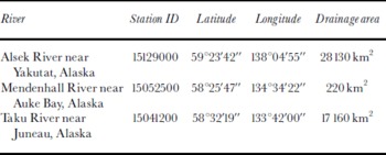
Discharge data for this region are sparse; three stations operated for most of the SSM/I period of record. Daily discharge values for two of these basins, the Alsek, Taku and Mendenhall Rivers, were supplied by the U. S. Geological Survey (seee http://water.usgs.gov/nwis/inventory/). The drainage basins vary greatly in size, average discharge and terrain characteristics (Table 2).
Table 2. Hydrologic station location information from the U.S. Geological Survey. Streamflow data are from http://water.usgs.gov/nwis/inventory
Near-surface air temperatures were acquired at 1191 m on the Juneau Icefield at Camp 10 (58.64° N, 134.20° W) using a Tempmentor instrument, which automatically recorded air temperature every 2 hours. The instrument was housed in a standard white meteorological shelter about 1.5 m above the nunatak surface.
Pixel Selection in Perennially Snow-Covered Regions
This section covers the selection of pixels that were analyzed, their terrain characteristics and their division into 11 geographic regions. Perennially snow-covered pixels in southeast Alaska were determined by overlaying EASE-Grid pixel centers with 37 km diameter circular regions over a 1986 late-summer (minimum snow cover) Landsat Thematic Mapper (TM) mosaic of the region, created from EROS Data Center, Sioux Falls, South Dakota, U.S.A. browse images. The mosaic was registered to a digital-elevation model (DEM) and geometrically rectified to the same projection as the SSM/I pixel-center coordinates (Fig. 1). Pixels included in this study were substantially snow-covered at the end of the summer melt season when the seasonal snowpack is at a minimum.
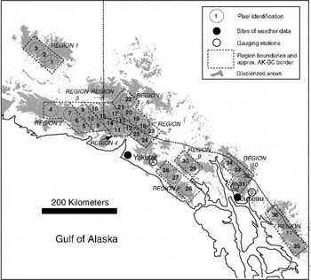
Fig. 1. Map of southeast Alaska showing the location and identification of the perennially snow-covered SSM/I pixels. Dashed lines outline the 11 geographic regions. Corresponding pixel information is given in Table 2. Small circles show sites where daily meteorological data and river discharge were recorded (A, Alsek River near Yakutat; B, Taku River near Juneau; C, Mendenhall River near Juneau).
Pixel locations and elevation distribution are shown in Figures 1 and 2. The 37 km diameter circle exceeds the EASE-Grid pixel dimensions in order to provide a more realistic scale of the satellite footprint. Topography, ground cover and melt state in this region vary substantially within a single pixel and imply heterogeneous emissions (Fig. 2). Twenty-seven of the 36 selected pixels are > 90% perennially snow-covered, covering an area of approximately 17000 km2. Two pixels with about 50% snow (at the minimum extent), and seven pixels with 80–90% snow were included. Elevations varied from 0–5795 m, and mean pixel elevations varied from 437–2442 m (Fig. 2).

Fig. 2. Histograms showing the altitude distribution for each pixel. Graphs are arranged by region and each plot is shown at the same scale. Elevation data come from the GTOPO30 DEM for Alaska. Pixel resolution is approximately 1 km × 0.5 km at this latitude.
Region definition and characteristics
Eleven regions were determined based on their geographic location. Each region consisted of two to five nearby pixels. Their distribution is shown in Figure 1 by dashed lines. Topography was captured in a histogram of elevations of the region surrounding each pixel center. These data are from the global digital elevation data (GTOPO30 DEM) with a 30 arc second grid (approximately 1 km × 0.5 km at this latitude). The histograms of pixel topographic distribution in each region are shown in Figure 2.
The 11 regions are numbered from northwest to southeast (Fig.1) and include the Wrangell Mountains (1), a high, inland range northwest of the rest of the study area; the western Bagley Icefield (2), source area for Miles and Bering Glaciers; and the upper Bagley Icefield, Yahtse Glacier and Guyot Glacier (3), which are east and inland of region 2. Elevations in region 1 range from 1000 to almost 5000 m with a mean of 2300 m. Region 2 is closer to the coast and considerably lower. Maximum elevations are about 3000 m. Region 3 has elevations as low as 600 m and ranges up to 5300 m. Region 4, still farther east, includes pixel 13 (Fig. 3), Seward Glacier, and the source area for Malaspina Glacier. The Malaspina piedmont lobe (southwest of pixel 11) is not included because it is a mixed pixel whose surface is mostly ice and rocky moraine, not snow, late in the melt season. Region 4 has a wide range of elevations from sea level to > 4200 m. It has the broadest range of all regions. Region 5 is north and inland of region 4 and the elevations are the highest in southeast Alaska and British Columbia. Region 5 has few elevations below 1500 m and extends up to the highest parts of the mountains at 5795 m. Region 6 is the most inland part of the Saint Elias Mountains that was analyzed. However, the Wrangell Mountains (region 1) are even farther inland.
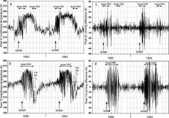
Fig. 3. 1992–93 time series of 37 GHz vertically polarized brightness temperature for each pixel (a, pixel 31; b, pixel 13) and 1992–93 time series of 37 GHz vertically polarized DAV (c, pixel 31; d, pixel 13). Vertical arrows mark approximate melt onset and decreased T b atthe onset offall conditions (refreeze and newsnow) foreach placeandyear. Horizontal arrowsshowduration of high DAV. The mean elevation of pixel 31 is 1217 m and of pixel 13 is 1810 m.
Regions 7–11 are lower-altitude icefields in southeast Alaska and British Columbia. They include the southeastern edge of the Saint Elias Mountains northeast of Yakutat (7) and the Fairweather Range and the Glacier National Wilderness (8). Many of the region 8 glaciers flow into Glacier Bay. Region 9 is east (inland) of region 8, in the Alsek Ranges and is also a source area for Glacier Bay. TheJuneau Icefield (10), a calibration site and the “Stikine Icefield” (11), southeast of Juneau in British Columbia, are the southernmost and east-ernmost areas studied. Among regions 7–11, with the exception of region 8, elevations are below 3000 m. Region 8 has a few elevations that reach up to 4200 m, but most of it is at low elevations. Pixel 26 may be mixed terrain and contaminated by sea water in the fiord.
Passive-Microwave Record
Seasonal patterns in passive-microwave signatures
The passive-microwave T b record is dependent on physical temperature and emissivity. Using the Raleigh–Jeans approximation, T b = ET s where T s is surface temperature and E is emissivity.
Individual pixels show a pronounced annual cycle in brightness temperature. By combining the day and night observations into a single chronological sequence, DAV, it is possible to see details in the snowpack dynamics. T b increases rapidly when the surface physical temperature approaches 0°C. This dramatic increase in T b has been attributed to the presence of liquid water in the snowpack. Similar sensitivity to liquid water in the snowpack in this region was also observed on synthetic-aperture-radar image sequences (Reference Smith, Forster, Isacks and HallSmith and others, 1997; Reference Ramage, Isacks and MillerRamage and others, 2000). Timing of the observed T b increase correlates well with year-round 2 hourly surface-temperature observations on the Juneau Icefield (see Reference Ramage and IsacksRamage and Isacks (2002) for further details of the physical mechanisms and technique).
Two melt regimes were identified in southeast Alaska, based on their summer melt characteristics: the “Taku regime” and the “Saint Elias regime”. The melt-onset signal is similar for both melt regimes. The presence of a small percentage of water causes high emissivity and, combined with the increase in snowpack T s, causes T b to increase significantly. The surface snowpack refreezes at night, forming an icy crust. Scattering from the icy surface causes T b to decrease well below the winter values. The alternation between high daytime T b due to melt conditions and low nighttime T b due to refrozen conditions yields high DAV. That makes the SSM/I combined ascending and descending data a good indicator of melt and refreeze dynamics.
Field studies of these processes were done by Reference MätzlerMätzler (1987) and Reference Mätzler and HüppiMätzler and Huppi (1989). Some regions continue to experience oscillations between melting and refreezing throughout the melt season. Snowpacks in other areas become isothermal and maintain a fairly high T b for much of the ablation season, indicating minimal ice-crust formation and more intense melting. These differences give rise to the Taku and Saint Elias regimes.
Some areas, such as the Juneau Icefield (region 10), showed a prominent melt onset characterized by increasing brightness temperature (T b) (Fig. 3a) and large DAV (Fig. 3c). Once snowmelt was well underway however, the DAV decreased to very small magnitudes (Fig. 3c). Field observations and temperature records indicate that most glacier surfaces in regions such as the Juneau Icefield stay continuously wet throughout the melt season. Once this occurs, the snow temperature and emissivity are uniform during both night and day. This is referred to as the Taku regime named for Taku Glacier, the main ice mass of the Juneau Icefield and site of the initial study and calibration data.
In contrast, high-altitude pixels, such as those in regions 4 and 5, did not experience a period of around-the-clock melt that is characterized in the passive microwave by high T b and continuously low DAV (Fig.3b and d). Rather, these high-altitude pixels maintained a very large DAV throughout the melt season indicating daily cycles of melt and refreeze. This type of melt-season cycle is called the Saint Elias regime after the Saint Elias Mountains (region 4).
Ablation magnitudes in these two environments are probably different. In the case of theTaku regime, low-amplitude DAV indicates that the snowpack was wet at both observation times. Thus, the surface need not remelt each day to start ablating. The number of hours per day when the snowpack was actively ablating was therefore greater than when nocturnal refreezing occurred. In the Saint Elias regime, the high DAV indicated recurring nocturnal freezes. Energy and time required to melt the surface snow made the daily ablation time shorter. The fact that the surface refroze for approximately half the time during the mid-summer ablation season suggests that the total ablation is smaller in the Saint Elias regime areas. These areas also had shorter overall ablation seasons than the Taku regime areas.
Two methods of analysis were developed previously to determine melt and refreeze (Reference Ramage and IsacksRamage and Isacks, 2002). In the following sections we use these methods to map the distribution of different melt regimes and to understand the interannual variations for the 11 southeast-Alaskan regions. Some regions show both melt regimes in different years, and are classified as an“intermediate melt regime”. Intermediate regions and regions that shifted from the Saint Elias regime to the Taku regime must have had highly variable year-to-year ablation magnitudes.
Detecting melt onset and refreeze
Brightness temperatures for perennially snow- and ice-covered surfaces (that melt during some portion of the year) have a bimodal distribution (Reference Ramage and IsacksRamage and Isacks, 2002). The two peaks correspond to frozen (low T b) and melting (high T b) surfaces. Because liquid water has such a dramatic effect on T b, there are fewer instances of intermediate T b values. The minimum between the two peaks was used to determine when pixels were likely to be melting. For this region, the threshold T b value used to identify snowmelt was 246 K. 246 ± 2 K is an appropriate threshold throughout southeast Alaska and appears to work in Greenland. There is little change in onset and refreeze dates with this threshold and 2 K margin. Changing the threshold by more than 2 K can result in incorrect or non-unique results. The value needs testing with field meteorological and snowpack data for use in other regions.
T b alone is not sufficient to identify melt periods. A T b threshold is used in conjunction with a DAV threshold to give a slightly different day and magnitude of melt onset. DAVare small (< ±10) when the surface stays frozen or stays wet and much larger (≫ ±10) when the surface alternates between frozen and melting. Adjusting the DAV threshold by −1 or +3 K would not substantially change the results. The DAV magnitude seems to be region-specific, so thresholds should be further tested in other regions.
We used two methods to estimate the melt onset, fall refreeze and ablation-season duration in southeast Alaska from 1988–98. For both methods, the onset and refreeze days were determined using a high resolution comparison of T b data (each half day was distinguishable), DAV magnitude and a cumulative plot on which a change in slope signified a change in melt condition.
The first (DAV) method uses only the diurnal-amplitude variations. This method records the whole period with liquid water in the surface snowpack at least part of the day and judges melt onset as the time when the DAV switches from low-amplitude (< ±10 K) to high-amplitude (> ±10 K) with the refreeze date chosen as the reversal back to small DAVat the end of the season. The second (melt) method considers simultaneous increases of brightness temperature and a high DAV. Melting measured by this method represents a warmer, wetter snowpack and occurs 10–20 days later than that measured by the DAV method.
For both methods, the ablation-season duration (in days) is the difference between the estimated refreeze date and the estimated onset date. There are synoptic variations in melt in all seasons. Ablation-season duration (in this usage) does not take into account individual days that may freeze during this period, nor does it take into account how much of the day, or how rapidly, the surface is melting.
Spatial and Temporal Variations
Interannual differences in snowmelt timing
We determined melt onset and refreeze timing for each pixel from 1988–98. Pixel dates were averaged for each region, and for all of southeast Alaska’s large glaciers. Average dates of melt onset and refreeze, and the ablation-season duration are shown in Figures 4–6. Figure 4a shows onset dates averaged for all 36 pixels. Trend lines are linear-fit lines and are shown for the southeast-Alaskan regional average of melt onset and refreeze date and the ablation-season duration of all regions. (Thick trend lines bracket the standard deviation to show the wide range of possible scenarios. R 2 values are shown.) Figure 5a shows average refreeze dates for the same period and Figure 6a shows the corresponding ablation-season duration. The regional average trends showed earlier melt onset (Fig. 4a), little trend in refreeze (Fig. 5a), and longer ablation seasons (Fig. 6a) in the most recent years of record. These characteristics lead to longer summer melting on southeast-Alaskan glaciers.

Fig. 4. Time series of melt-onset date for (a) southeast-Alaskan regional average and each of the 11 study regions (b–l). Both the DAV method (black dots) and the melt method (open circles) are shown. A linear fit trend is shown only for the southeast-Alaskan average.
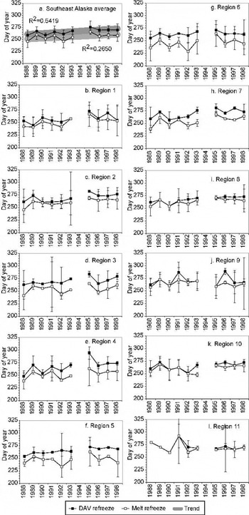
Fig. 5. Same as Figure 4 showing time series of refreeze date.

Fig. 6. Same as Figure 4 showing time series of ablation-season duration.
Average onset and refreeze for each of the 11 southeast-Alaskan regions are shown in Figures 4b–l and 5b–l, respectively. Error bars show one standard deviation for each region. Note the small sample size of some regions (especially 9 and 11). The error bars are large for years in which there were more missing data and in some cases for regions with few pixels. The regional trends are shown as thick lines to encompass that uncertainty. Uncertainties for individual pixels ranged from ±1 to ±8 days. Time series for individual pixels are shown in Reference RamageRamage (2001). All 11 regions showed earlier melt onset toward the later part of the 1988–98 period (Fig. 4). Refreeze dates were variable, but most individual regions showed no obvious trend (Fig. 5). As a result, the ablation-season length was dependent on the timing of melt onset. Ablation-season length, for all regions, showed a trend toward increasing length in the later 1990s (Fig. 6).
Both methods for assessing season timing and length show that there is wide variability in southeast-Alaskan snowmelt patterns from year to year. The ablation-season-duration graphs are not monotonic curves and the trends should be considered with caution. Figures 4 and 5 show the regional onset and refreeze dates and their standard deviations. The thick lines represent the range of dates and emphasize that there is a wide variability within this short record. We are cautious in our interpretation because there was substantial year-to-year variability, the period of observation was only 11 years and in some cases the R 2 values were not high. In most, but not all, cases the DAV method and the melt method yielded parallel results on both a yearly and a decadal scale.
Spatial differences in snowmelt timing
A major factor affecting the timing of the melt onset is the altitude. It affects both the style of summer melt and the timing and duration of melt. Figure 7 shows a comparison of the melt onset (Fig. 7a, c and e) and the ablation-season duration (Fig. 7b, d and f) for the 11 southeast-Alaskan regions over time. The regions are divided into three groups based on mean elevation. These comparisons show two patterns. First, it is noticeable that onset date is earlier at lower altitudes and later at high altitudes. Thus, and not surprisingly, ablation-season duration decreases with an increase in altitude. Regions in Figure 7a and b melt later and for less time than regions in Figure 7c–f. Second, as the altitude increased, so did the difference between the two methods of observing meltwater in the snowpack. This difference is important for the hydrology and mass exchange at the surface, because not only is spring later to arrive at high altitudes, but it is also slower to intensify and likely to end earlier. In almost all regions (and using either melt method), the tendency is for the melt season to increase in length over the time period of 1988–98.
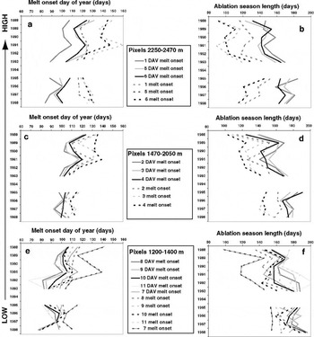
Fig. 7. Time series of melt-onset date and ablation-season duration. The regions are divided into three groups based on mean elevation and arranged from highest elevation (a, b) to moderate elevation (c, d) to lowest elevation (e, f). Numbers refer to regions. The day of year is along the x axis, and the year is along the y axis starting with 1988 at the top. Both the DAV (solid lines) and melt (dashed lines) methods are shown. Colors correspond to each region. No dates are shown for 1994 because there are so few SSM/I data. Regions 1, 5 and 6 (a, b); regions 2, 3 and 4 (c, d); and regions 7–11(e, f).
The difference between the DAV and the melt methods was much greater in some regions than in other regions. Regions 2 and 7–11 have small differences in onset dates (Fig. 4c and h compared to Fig. 4a and d–g). The two methods have similar refreeze dates (Fig. 4c and h). Each of these regions is a fairly low-elevation location and close to the coast.
Intensity of the melt season
One other way of assessing regional temporal and spatial variations is to look at the melt regime. The DAV method and the melt method focused on the beginning and end of melting based on the brightness signature of diurnal melt-refreeze cycles. In the case of pixels such as pixel 13 in the Saint Elias Mountains, the high-magnitude DAV persisted throughout the season (Fig. 3b and d). However, on the Juneau Icefield, once the melt intensity increased sufficiently, the diurnal cycles ceased or became small (Fig. 3a and c). On maritime pixels like the Juneau Icefield (Taku regime), this high T b but low-DAV time period corresponds to the time of highest ablation rate. Some pixels display either Taku or Saint Elias regime characteristics in different years and these are classified as “intermediate.”
Figure 8 shows the spatial distribution of these three types of pixels. Black circles are pixels that consistently exhibit Taku melt-regime characteristics (Fig. 3a and c). White circles are consistently Saint Elias melt regime (Fig. 3b and d) and gray pixels show either Taku or Saint Elias regimes each about half the time. The distribution of regime type is related to altitude (Fig. 9). All Taku regime pixels have a mean elevation below 1600 m. The Saint Elias regime mean pixel elevations range from 1400–2600 m. The intermediate pixels also have a wide range in altitude (1320–2350 m), and are not exclusively dependent on altitude for their characteristics. The Wrangell Mountains (region1) are in the intermediate regime, but they are also some of the highest pixels.
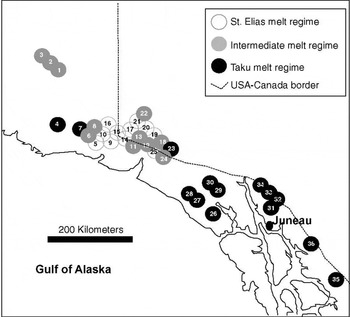
Fig. 8. Study region showing the melt regime of each EASE-Grid SSM/I pixel. Snow cover that becomes isothermal and does not display daily melt–refreeze characteristics throughout the melt season is classified as Taku melt regime (black). Pixels that maintain the diurnal cycles (large-amplitude DAV) throughout the summer are classified as Saint Elias melt regime (white). Pixels that varied between melt regimes are classified as intermediate (gray).
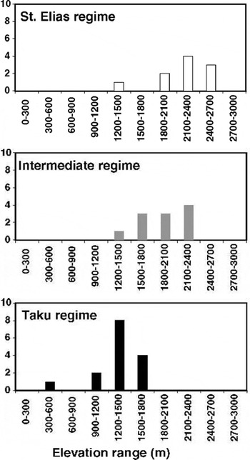
Fig. 9. Histograms showing distribution with elevation of Taku, intermediate, and Saint Elias melt regimes. Values shown are mean elevations. Elevation distributions are shown in Figure 2.
There is an indication that not only the ablation-season duration, but the melt intensity may have increased between 1988 and 1998 on high-altitude (Saint Elias regime) pixels. Throughout the coldest parts of the study region, where pixels are uniformly characterized by summer-long daily refreeze cycles, both in 1995 and 1997 the middle of the summer behaved like the Taku regime, particularly pixels 9, 12 and 13 (Reference RamageRamage, 2001). The decadal time period is too short to assess whether this is a shift in regime or an example of a summer with very wet snow. If there has been a shift toward more regions in the Taku melt regime, it may have had a significant influence on net ablation throughout the region. It is also possible that 1995 and 1997 showed the warmer end of an interval of natural variability. A longer time series will be necessary to distinguish these possibilities. In either case, a good question is “What was happening in 1995 and 1997 that made regions 3–6 melt more intensely than they did in the other 8 years of observation?”
Southeast-Alaskan Hydrology
Gauging-station locations
Few locations in southeast Alaska were gauged from 1988–98 when satellite monitoring was underway. Three gauging stations within the study area that include fully or partially glacierized catchments operated during the period of SSM/I record (1987–98) (Table 2). Only the Mendenhall River station measures mainly glacial discharge (with a small component from surrounding mountainsides). The other, larger drainage areas include some glacier and perennially snow-covered pixels of interest and large areas covered only by seasonal snow.
In this section, we describe the seasonal hydrology of the region based on gauge data from the U. S. Geological Survey, differences between the basin characteristics, and the relationship of the discharge curves to seasonal snowmelt progression and nearby precipitation records. We also evaluate the interannual signal from the Mendenhall River discharge record. The hydrographs and SSM/I record show the connection between the stages of seasonal and glacier snowmelt and the associated river discharge.
Seasonal hydrology, station variations and precipitation
Characteristics of southeast-Alaskan river basins are low winter flow, an initial increase in discharge at about days 100–110, a steep increase starting about day130, and a decrease to a stable, low winter flow (starting at day 320 in 1993). Alsek and Taku River flows decrease in late summer after day 200, whereas the Mendenhall flow continues to be high and does not decrease after day 200. Due to continued glacier melt or meltwater storage, the Mendenhall River discharge remains high until much later in the season. The low winter flow is perturbed occasionally by large precipitation events (Fig. 10c and f) recorded at Juneau and Yakutat airports, both near sea level and on the coast. Short-lived discharge peaks above the seasonal curve were related to precipitation events (Fig. 10). Rain during periods when the temperature was > 0°C caused discharge peaks.

Fig. 10. Comparison among 1993 icefield DAV, river discharge and precipitation. (a) Pixel 31 DAV; (b) Mendenhall River discharge; (c) daily precipitation at Juneau airport; (d) pixel 28 DAV; (e) Alsek River discharge; and (f) daily precipitation atYakutat airport.
The increase in river discharge near day 130 was very rapid. In 1993 (Fig. 10) there were two stages of discharge increase (starting at days100 and 130), but some other years show an approximately exponential increase for about a month in April or May (days 100–150; Fig. 11). The initial rise in discharge sometimes reached high, sustained peaks that were tied more to snowmelt runoff than to precipitation events. Summer maxima varied, but many of the short-lived spikes in meltwater runoff corresponded to precipitation. This left a large flow component that reflected the season’s snow and glacier melt.

Fig. 11. Comparison of SSM/I DAV on the Juneau Icefield (pixel 31) with discharge from Mendenhall River (1988–90, 1991–93, 1997–98). Pixel 31 makes up much of the drainage area of Mendenhall Glacier, and therefore the Mendenhall River. (a) 1988 DAV; (b) 1988 discharge; (c) 1989 DAV; (d) 1989 discharge; (e) 1990 DAV; (f) 1990 discharge; (g) 1991 DAV; (h) 1991 discharge; (i) 1992 DAV; (j) 1992 discharge; (k) 1993 DAV; (l) 1993 discharge; (m) 1997 DAV; (n) 1997 discharge; (o) 1998 DAV; and (p) 1998 discharge. Vertical lines on the DAV plots show onset based on DAV threshold, melt thresholds and the end of the high-DAV period in spring. Vertical lines on the discharge plots show the initial discharge increase in spring and the point at which the discharge exceeded 57 m3 s1
The early spring discharge increase corresponded to the beginning of the melt season (Fig. 10). The Alsek River peaked and then declined after the seasonal snow cover had melted away (Fig. 10e). These distinct characteristics of the river discharge reinforce the SSM/I snowmelt-pattern correspondence with the physical state of the snowpack, as discussed in detail below.
The seasonal discharge declined in the late summer and fall, at the same time as the precipitation increased in both frequency and magnitude (days 220–365; Fig. 10). This decline is attributed to the fact that the seasonal snow cover has melted off, so the primary contributions are glacier melt and precipitation and the shift from rain to snow at higher elevations as the next accumulation season sets in. The diurnal-amplitude variations that are important for determining melt timing relate well to river discharge.
Discharge relation to SSM/I snowmelt record and interannual variations
Melt-onset timing based on both DAVand melt methods was corroborated based on regional river discharge records. The discharge curves help interpret what the changes in DAV signify about snowpack ripening and release of water to the hydrologic system. The calibration site was Mendenhall River, a drainage basin that has primarily glacial discharge and includes much of pixel 31 in its headwaters. Discharge curves have a rapid increase in early spring that is close in time to the SSM/I-derived melt-onset dates (Fig. 11). The discharge responded rapidly to the seasonal and glacial snowmelt. DAV-method melt onset on pixel 31 occurred near the earliest indication of an increase in annual discharge, with the exception of the occasional winter spike due to rain. Dates for the two methods were similar for the sites where both discharge and SSM/I data were available.
Both the beginning and the end of the period of high diurnal T b variability correspond to important points in basin hydrology. In mid March 1993 (∼ day 130) the discharge on the Mendenhall River reached a significant and prolonged peak coincident with the end of the high-DAV period (Figs 10 and 11). The increase and rate of change was much greater than from precipitation alone. Discharge reached approximately 57 m3 s−1 at about the time of the end of the spring DAV. The significant discharge increases come at the end of the period of frequent melt–refreeze cycles (Figs 10 and 11). This relationship shows that although the beginning of high DAV corresponds with the onset of melting, the end of high spring DAV (inTaku regime areas) corresponds to the time when the snowpack has started to release a large amount of meltwater that has flowed downstream to the gauging station. Pixel 31 DAV is compared to the glacierized Mendenhall River basin discharge for the overlapping years of record (1988–93, 1997, 1998) (Fig. 11).
Interannual variations in Mendenhall River discharge curves are compared to the region 10 DAVonset, end of high DAV and melt onset (Fig. 12). The initial increases in discharge are similar to the DAV-onset dates in most years. The discharge started earlier in 1991 and was delayed in 1997 and 1998. Flow increased rapidly for the month following initial increases. The dates when discharge increased to 57 m3 s−1 are compared to the dates of the end of the high-DAV period. The dates are similar though there is variation in whether DAV precedes the discharge level or not.

Fig. 12. Interannual variation of snowmelt onset based on the DAV and melt methods on Juneau Icefield (pixel 31) compared to downstream river discharge.
The end of the high-DAV period coincides with the rapid rise in meltwater. On Mendenhall River there is even more discharge after the high DAV, when the glacier is releasing meltwater during the day and night, as is evidenced by the return to small DAV on Juneau Icefield. During this time discharge continues to be high or increase throughout the melt season because Mendenhall River is fed by glacier runoff. The Alsek and Taku Rivers are drainage systems with a large area of seasonal snow cover in addition to some glaciated areas. The end of high DAV on pixels within each drainage basin corresponds with a major increase in runoff that is not maintained throughout the melt season. Discharge from these three rivers with extensive snow and glaciers in their basins gives a strong indication that the SSM/I melt-onset methods are capturing real transitions in the snowmelt cycle, in particular melt onset, snowpack ripening and water release to channel flow.
Temperature variability and snowmelt
The Juneau and Yakutat airports are the nearest long-term weather stations to compare with SSM/I snowmelt observations. Both weather stations are near sea level. Since regional lapse rates are spatially and temporally variable, we made no attempt to relate the actual temperatures to those on the nearby icefields. However, these temperature and precipitation records represent the relative temperature and precipitation in different months and years. The temperature observations relate more directly to SSM/I snowmelt timing and magnitude than do the precipitation observations.
Monthly means of the daily maximum and minimum temperatures were used to compute monthly temperature anomalies for each calendar year. The monthly anomalies are based on the mean monthly temperatures for 1985–98 (Fig. 13). A positive anomaly means that the average temperature for the month was higher than the average temperature for the same month averaged over the 14 year period.

Fig. 13. Comparison of melt-onset dates for regions 4, 7 and 10 with April and May mean-monthly temperature anomalies 1988–98. (a) Region 10 compared to Juneau temperature; and (b) regions 4 and 7 compared to Yakutat temperature. Note that the temperature scale is reversed in sign.
The melt-onset dates are explainable by looking at the monthly temperature anomalies through time. There are similarities between the monthly temperature anomalies and the timing of melt onset. On Juneau Icefield (region 10), higher than average April temperature anomalies correlate well with early melt-onset dates (Fig. 13a). In Figure 13, the melt-onset date is shown on the left y axis and temperature anomalies are shown in °C on the right y axis (note that the temperature scale is reversed). The regions closest to Yakutat (regions 4 and 7) are compared to average April and May temperature anomalies (Fig. 13b). The Yakutat temperature anomalies in April and May also had similar trends to the onset dates in most years.1990 and 1995 do not correlate well.
There are a few years in which high-elevation Saint Elias pixels show theTaku melt regime. We interpreted these as years with intense melting for a period, even on the highelevation pixels. There is a correspondence between years with high July or August temperature anomalies and the Taku regime snowmelt on Saint Elias regime pixels. The high temperatures may be a factor in the switch from a regime of diurnal refreeze in mid summer to a regime with continually wet snow. Temperature anomalies for those years were high in the summer months. This correspondence between higher than normal August temperatures and the Taku melt regime suggests that the temperature is at least one major factor in driving the different melt regimes on high icefields, and that it is feasible to use the SSM/I to interpret the seasonal-melt intensity.
Conclusions and Future Work
SSM/I brightness temperatures and diurnal-amplitude variations were used to determine melt-onset date, refreeze date and the duration of the ablation season for 36 perennially snow-covered pixels located on glaciers in southeast Alaska. There are large interannual variations in the timing of melt onset, refreeze and duration of the ablation season. Averages for 11 geographic regions within southeast Alaska show probable trends toward earlier melt onset and longer ablation seasons in the later part of the period from 1988–98. The average for all the regions within southeast Alaska that were observed from 1988–98 shows an earlier melt-on-set date and a longer ablation season. Regions also show a slight trend toward a later refreeze, but this is not as widespread nor a strong signal. Timing of onset and length of ablation season are closely related to altitude and seem to be affected by proximity to the coast. Pixels at higher altitude melt later and for a shorter season than those at low elevations. The timing and regime of melting can be monitored using this method. High-altitude sites tend to exhibit Saint Elias melt-regime characteristics.
Melt-onset timing, from both DAV and melt methods, was corroborated based on regional river discharge records for a period that overlapped with SSM/I coverage. Mendenhall River is fed by glacier runoff; during the summer melt season, discharge continues to be high or increase throughout the melt season. Alsek River has a large drainage area of seasonal snow cover, in addition to some glacierized areas, so the end of high DAV corresponds with a major increase in runoff that is not maintained throughout the melt season. Discharge curves have a rapid increase in early spring that is similar to the SSM/I-derived melt-onset dates. The discharge responds rapidly to the seasonal and glacial snowmelt and increases in just days from melt onset. The sensitivity and rate depend on per cent of the pixel melting, basin size and meltwater-flow paths. This relationship shows that the beginning of high DAVcorresponds with the onset of melting, and the end of high spring DAV (in Taku regime areas) corresponds to the time when the snowpack has started to release a large amount of meltwater that has flowed rapidly downstream to the gauging station. The T b and DAV give information about melt onset, snowpack ripening, and water release to channel flow. Discharge from these three rivers, with extensive snow and glaciers in their basins, indicates that these SSM/I melt-onset methods are capturing real transitions in the snowmelt cycle. Further fieldwork is needed to fully understand the precise physical state of the snowpack moisture represented by each of these two methods.
Regional differences in the passive-microwave brightness-temperature signatures indicated that it is possible to characterize the melt regime of different pixels. The brightness-temperature signatures also differ for regions at different altitudes and distance from the coast. Fourteen pixels exhibit Taku regime melt characteristics and 11 pixels exhibit Saint Elias regime melt characteristics. The remaining 11 pixels are classified as intermediate because they seem to show either Taku or Saint Elias regime characteristics in different years. Some areas change from one melt regime to another. Shifts in melt regime probably have a major influence on net ablation in those regions. Because the record is only 11 years, it is not known whether the regime shift is part of a longer-term pattern or an actual change due to a regional climate oscillation or global warming.
Temperature is a major factor driving melt regime and volume. High mean-monthly temperature anomalies for July and August correspond with the more intense melt regimes. The temperature anomalies may be a factor in causing a change from the diurnal refreeze in Saint Elias regime regions to Taku regime. The causes for the observed melt-onset and refreeze-timing variability and possible trends will be studied in more detail using both surface observations on Alaskan glaciers and a coupled glacier–atmosphere mesoscale model.
Acknowledgements
SSM/I EASE-Grid satellite data come from the National Snow and Ice Data Center in Boulder, Colorado. We would like to thank M. M. Miller, A. C. Pinchak, R. Asher and the Juneau Icefield Research Program for use of meteorological data. Discharge data were supplied by the U.S. Geological Survey. Precipitation data come from the U.S. National Oceanic and Atmospheric Administration. Two anonymous reviewers provided helpful suggestions. This research was supported by a U.S. National Aeronautics and Space Administration (NASA) Graduate Student Researcher Program/Goddard Space Flight Center grant NGT5-51 and NASA Land Surface Hydrology Program grant NAG5-7497 and the Clare Boothe Luce Program of the Henry Luce Foundation.


