


1. Introduction
Recently, low-Reynolds-number flow operating at  $Re\sim O(10^{4})$ has drawn much attention due to a variety of engineering and industrial applications. Examples include small- to medium-scale wind turbines (Tangler & Somers Reference Tangler and Somers1995), unmanned aerial vehicles (Carmichael Reference Carmichael1981; Mueller & DeLaurier Reference Mueller and DeLaurier2003), and recently, the Mars explorer (Kojima et al. Reference Kojima, Nonomura, Oyama and Fujii2012; Anyoji et al. Reference Anyoji, Nonomura, Aono, Oyama, Fujii, Nagai and Asai2014). A very important feature in this flow regime is laminar separation and the transition to turbulence, leading to various flow patterns that can pose direct impact on drag and lift. It has been studied extensively that at flow conditions that are sufficiently turbulent and with low angle of attack, flow can recover sufficient energy through entrainment to reattach to the aerofoil surface, forming a recirculation bubble in the time-averaged flow, namely the laminar separation bubble (LSB). Recently, large-eddy simulations (LES) and direct numerical simulations (DNS) have been used extensively to study detailed turbulent flow structures on aerofoils. In the low-Reynolds-number cases, considerable research effort has been put into the separation, detachment and LSB in low angle of attack cases (e.g. Shan, Jiang & Liu Reference Shan, Jiang and Liu2005; Jones, Sandberg & Sandham Reference Jones, Sandberg and Sandham2008). Moreover, to optimize the design of the aircraft-like device operated in the thin Mars atmosphere, a series of LES were conducted by Kojima et al. (Reference Kojima, Nonomura, Oyama and Fujii2012) and Anyoji et al. (Reference Anyoji, Nonomura, Aono, Oyama, Fujii, Nagai and Asai2014) to examine the performance of different types of aerofoil sections in different angles of attack. Taking advantage of modern computational power, these high-fidelity numerical studies revealed spectacular details of flows in transition and turbulent regimes, providing valuable information on the fine-scale flow structures around aerofoils at low-Reynolds-number flows. However, direct and quantitative measures of the connection of these flow structures and the resulting force contribution are still lacking. Such quantitative measures may also have great benefit for flow control on aerofoils.
Studying the force acting on a submerged body has been a crucial area of research in fluid mechanics. Past studies aimed to break down the resultant forces into components associated with different aspects of fluid flow. In earlier days, circulation theory was utilized to establish a relationship between forces and inviscid models (e.g. Howarth Reference Howarth1935; Sears Reference Sears1956, Reference Sears1976), while later studies focused on providing exact means or theories for the relationship between hydrodynamic forces and surrounding flow fields through rigorous analyses of the equation for viscous flow (e.g. Kambe Reference Kambe1986; Howe Reference Howe1995; Wells Reference Wells1996; Howe, Lauchle & Wang Reference Howe, Lauchle and Wang2001). In this study, the force representation theory proposed by Chang (Reference Chang1992) is employed to obtain force resultants due to the flow field. Based on the d’Alembert paradox, Quartapelle & Napolitano (Reference Quartapelle and Napolitano1983) first derived alternative expressions for force and moment by projecting the momentum equations onto the gradient of the auxiliary velocity potential. Chang (Reference Chang1992) further related the force on the moving, accelerating or oscillating body to different aspects of the flow field. This theory states that any real fluid element with non-zero vorticity can be considered a source of the hydrodynamic force, and has been applied to understand forces exerted on various objects in low-Reynolds-number flows ( $Re\sim O(10\unicode{x2013}100)$), such as flow passing multiple bluff bodies (Chang, Yang & Chu Reference Chang, Yang and Chu2008; Wang et al. Reference Wang, Zhao, Graham and Li2022), hovering flights (Hsieh, Chang & Chu Reference Hsieh, Chang and Chu2009; Hsieh et al. Reference Hsieh, Kung, Chang and Chu2010), impulsively started finite plates (Lee et al. Reference Lee, Hsieh, Chang and Chu2012), and the heaving aerofoil (Martín-Alcántara, Fernandez-Feria & Sanmiguel-Rojas Reference Martín-Alcántara, Fernandez-Feria and Sanmiguel-Rojas2015; Moriche, Flores & García-Villalba Reference Moriche, Flores and García-Villalba2017). As the Reynolds number increases to a level where turbulence becomes a significant factor (
 $Re\sim O(10^{4})$), we become curious about how the irregularities of turbulence impact the forces acting on an object. Although force representation theory had been extended to study the hydrodynamic forces on aerofoils in cavitation flows using the Reynolds-averaged Navier–Stokes equations (Shen et al. Reference Shen, Li, Li, Wang and Liu2021), they have examined only the large-scale motions due to the smearing of small eddies by the averaged flow field. Therefore, there is still a lack of research in the scientific community on the contributions of small-scale turbulent structures to drag and lift forces.
In order to identify the characteristic eddies in turbulent flows, various techniques are available. These include proper orthogonal decomposition (POD) proposed by Lumley (Reference Lumley1967, Reference Lumley1970), dynamic mode decomposition introduced by Schmid (Reference Schmid2010), and resolvent analysis by McKeon & Sharma (Reference McKeon and Sharma2010). Among these, the most commonly used approach is POD, where the main objective is to identify the most effective approach for capturing the dominant components of an infinite-dimensional stochastic process. An inexpensive implementation developed by Sirovich (Reference Sirovich1987) involves the decomposition of the autocorrelation function of flow variables, resulting in spatially orthogonal modes that are modulated temporally by expansion coefficients. This approach, known as space-only POD, has found extensive application in addressing turbulence-related issues such as turbulence channel flow (Moin & Moser Reference Moin and Moser1989), turbulence jets (Freund & Colonius Reference Freund and Colonius2009), and acoustic effects on aerofoils (Ribeiro & Wolf Reference Ribeiro and Wolf2017). However, it is well known that typically, characteristic eddies contain coherence in both space and time (Pope Reference Pope2000), while the space-only POD simply provides modes that are correlated with space. To address this issue, Towne, Schmidt & Colonius (Reference Towne, Schmidt and Colonius2018) adopted the mathematical framework proposed by Lumley (Reference Lumley1967, Reference Lumley1970) and developed a novel algorithm to deal with the spectral eigenvalue problem of cross-spectral density. This particular variant of POD is referred to as spectral POD (SPOD) (Picard & Delville Reference Picard and Delville2000), which guarantees that modes oscillating at a single frequency are mutually orthogonal. This property makes SPOD particularly suitable for identifying coherent structures that are physically significant in problems such as those mentioned above, e.g. channel flow (Tissot, Cavalieri & Mémin Reference Tissot, Cavalieri and Mémin2021), jet (Schmidt et al. Reference Schmidt, Towne, Rigas, Colonius and Brès2018) and acoustic Abreu et al. Reference Abreu, Tanarro, Cavalieri, Schlatter, Vinuesa, Hanifi and Henningson2021).
In this work, we investigate the fundamental physics behind flow over the NACA0012 aerofoil with different angles of attack ( $AoA=7.5^{\circ }$ and
  $10^{\circ }$). Numerical simulations are conducted using LES of incompressible flow at a chord Reynolds number
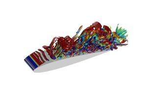
  $Re=50\,000$, and the snapshots of simulation results are dealt with by SPOD to obtain the coherent structures in the frequency domain. We then apply a reconstruction technique proposed by Nekkanti & Schmidt (Reference Nekkanti and Schmidt2021) to convert these coherent structures back into the time domain. The novelty of this study is that contributions of each SPOD mode to drag and lift forces can be quantified by force representation theory. This brings us an insight to verify the importance of the associated coherent structures and to reduce the complexity of the original flow fields. Since a SPOD mode involves motions with various frequencies, the proposed method can further decompose the effect of SPOD modes oscillating at certain frequencies on drag and lift forces. With these simplified flow fields, variations of both drag and lift forces caused by the vorticity within the domain can be identified clearly. To the best of our knowledge, this is the first research to provide quantitative analysis of the coherent structures in turbulence flows, and the basic understanding of SPOD modes is helpful for the design of aircraft and flow control.
The rest of the paper is organized as follows. Section 2 presents the details of force representation theory. In § 3, we introduce the implementations of SPOD and the SPOD-based flow field reconstruction. Section 4 shows the numerical methods and validations. The simulation results are demonstrated in § 5. The effects of SPOD modes on aerodynamic forces and their vorticity forces are presented in §§ 6 and 7. Finally, concluding remarks are summarized in § 8.
2. Vorticity force representation
In the framework of LES, the flow is governed by the spatial-filtered incompressible Navier–Stokes equation, which is written in dimensionless form as
 \begin{gather} \boldsymbol{\nabla} \boldsymbol{\cdot} \bar{\boldsymbol{u}} = 0,\quad \dfrac{\partial \bar{\boldsymbol{u}}}{\partial t} + \boldsymbol{\nabla} \boldsymbol{\cdot} (\bar{\boldsymbol{u}}\otimes \bar{\boldsymbol{u}}) =-\boldsymbol{\nabla} \bar{p} + \dfrac{1}{Re}\, \nabla^2 \bar{\boldsymbol{u}} - \boldsymbol{\nabla} \boldsymbol{\cdot} \boldsymbol{\tau}_{{SGS}}, \end{gather}
where  $\bar {\boldsymbol {u}}$ and
  $\bar {\boldsymbol {p}}$ denote the spatial-filtered quantities of flow velocity and pressure,
  $Re=U_{\infty }L/\nu$ is the Reynolds number (in which
  $U_{\infty }$ is the free stream velocity,
  $L$ is the chord length of the aerofoil, and
  $\nu$ is the kinematic viscosity), and
  $\boldsymbol {\tau }_{{SGS}}$ is the subgrid-scale (SGS) stress that needs to be reconstructed. Typically, the drag and lift forces exerted on the aerofoil are comprised of the pressure force and skin friction:
 $$\begin{gather} {F}_{{D}} = \int_{S_{w}} \bar{p}(\boldsymbol{n}\boldsymbol{\cdot}\boldsymbol{i})\,{\rm d}A + \dfrac{1}{Re}\int_{S_{w}} (\boldsymbol{n}\times \bar{\boldsymbol{\omega}})\boldsymbol{\cdot}\boldsymbol{i}\,{\rm d}A, \end{gather}$$
 $$\begin{gather}{F}_{{L}} = \int_{S_{w}} \bar{p}(\boldsymbol{n}\boldsymbol{\cdot}\boldsymbol{j})\,{\rm d}A + \dfrac{1}{Re}\int_{S_{w}} (\boldsymbol{n}\times \bar{\boldsymbol{\omega}})\boldsymbol{\cdot}\boldsymbol{j}\,{\rm d}A, \end{gather}$$
where  ${F}_{{D}}$ and
  ${F}_{{L}}$ are lift and drag forces,
  $S_{w}$ is the surface of the aerofoil,
  $\boldsymbol {n}$ is the normal vector pointing inwards from the aerofoil,
  $\boldsymbol {i}$ and
  $\boldsymbol {j}$ represent the unit vectors in the drag and lift directions, and
  $\bar {\boldsymbol {\omega }}=\boldsymbol {\nabla }\times \bar {\boldsymbol {u}}$ is the vorticity of the flow field. In this study, an alternative way to obtain the drag force in (2.2) is vorticity force analysis derived by Chang (Reference Chang1992). In his derivation, an auxiliary potential function
  $\phi _{1}$ is introduced to satisfy the Laplace equation and the boundary conditions:
 \begin{gather} \nabla^{2}\phi_{1} = 0, \end{gather}
 \begin{gather} \boldsymbol{\nabla}\phi_{1}\boldsymbol{\cdot}\boldsymbol{n} =-\boldsymbol{i}\boldsymbol{\cdot}\boldsymbol{n}, \quad \boldsymbol{x} \ \mbox{on}\ S_{w}, \end{gather}
 \begin{gather} \phi_{1} = 0, \quad \boldsymbol{x}\rightarrow \pm \infty. \end{gather}
Equations (2.4)–(2.6) reveal that  $\phi _{1}$ is the potential flow induced by a translational motion of the aerofoil at unit speed in the drag direction, and
  $\boldsymbol {\nabla }\phi _{1}$ denotes the velocity field corresponding to such a flow condition. In the present study, we solved (2.4) numerically within the domain shown in figure 1. Here, we assumed that the outer boundary
  $S_{R}$ is far enough from the aerofoil such that (2.6) can be approximated as
 \begin{equation} \phi_{1} = 0,\quad \boldsymbol{x}\ \mbox{on}\ S_{R}. \end{equation}
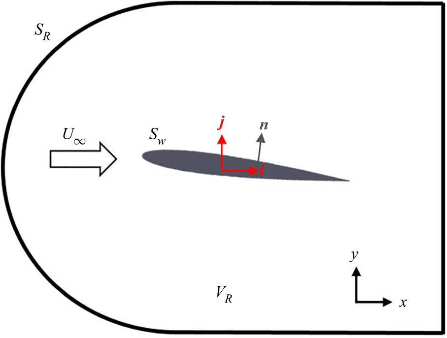
Figure 1. Schematic showing the configuration of vorticity force analysis, where  $V_{R}$ is the control volume,
  ${S_{w}}$ is the surface of the aerofoil,
  ${S_{R}}$ is the cuboid surface of the control volume,
  $U_{\infty }$ is the free stream velocity,
  $\boldsymbol {n}$ is the normal vector of the aerofoil, and
  $\boldsymbol {i},\boldsymbol {j}$ are the unit vectors in the drag and lift directions, respectively.
Figures 2(a,c) show  $\phi _{1}$ zoomed in at the aerofoil used in the present cases with
  $AoA=7.5^{\circ }$ and
  $10^{\circ }$. Now we rewrite the advection and viscous terms in (2.1a,b) using the following two vector identities:
 $$\begin{gather} \bar{\boldsymbol{u}}\boldsymbol{\cdot}\boldsymbol{\nabla}{\bar{\boldsymbol{u}}} = \tfrac{1}{2}\,\boldsymbol{\nabla}\vert\bar{\boldsymbol{u}}\vert^2-\bar{\boldsymbol{u}}\times\bar{\boldsymbol{\omega}}, \end{gather}$$
 $$\begin{gather}\nabla^2\bar{\boldsymbol{u}}= \boldsymbol{\nabla}(\boldsymbol{\nabla}\boldsymbol{\cdot}\bar{\boldsymbol{u}})-\boldsymbol{\nabla}\times\bar{\boldsymbol{\omega}}=-\boldsymbol{\nabla}\times\bar{\boldsymbol{\omega}}, \end{gather}$$
and the resulting momentum equation becomes
 \begin{equation} {-\boldsymbol{\nabla}}\bar{p} = \dfrac{\partial\bar{\boldsymbol{u}}}{\partial t}+\dfrac{1}{2}\,\boldsymbol{\nabla}\vert\bar{\boldsymbol{u}}\vert^2-\bar{\boldsymbol{u}}\times\bar{\boldsymbol{\omega}}+\dfrac{1}{Re}\,(\boldsymbol{\nabla}\times\bar{\boldsymbol{\omega}})+\boldsymbol{\nabla}\boldsymbol{\cdot}\boldsymbol{\tau}_{SGS}. \end{equation}
Taking an inner product with  $\boldsymbol {\nabla }\phi _{1}$ on both sides of (2.10) within control volume
  $V_{R}$ (see figure 1), and substituting (2.1a,b) and (2.4)–(2.6), along with the Gauss divergence theorem, yields
 $$\begin{gather} \int_{S_w}\bar{p}(\boldsymbol{n}\boldsymbol{\cdot} \boldsymbol{i}) \,{\rm d}A =\int_{S_w} \phi_1\,\dfrac{\partial \bar{\boldsymbol{u}}}{\partial t}\boldsymbol{\cdot} \boldsymbol{n}\,{\rm d}A - \dfrac{1}{2}\int_{S_w }\vert \bar{\boldsymbol{u}} \vert^2 \boldsymbol{n}\boldsymbol{\cdot} \boldsymbol{i}\,{\rm d}A\nonumber\\ {}-\int_{V_R}\bar{\boldsymbol{u}}\times \bar{\boldsymbol{\omega}}\boldsymbol{\cdot} \boldsymbol{\nabla} \phi_1 \,{\rm d}V +\dfrac{1}{Re}\int_{S_w}\boldsymbol{n}\times\bar{\boldsymbol{\omega}}\boldsymbol{\cdot} \boldsymbol{\nabla}\phi_1 \,{\rm d}A +\int_{V_R}\boldsymbol{\nabla} \boldsymbol{\cdot} \boldsymbol{\tau}_{SGS} \boldsymbol{\cdot} \boldsymbol{\nabla} \phi_1 \,{\rm d}V, \end{gather}$$
where  $S_{R}$ is the cuboid surface of the control volume. It should be noticed that since
  $\boldsymbol {\nabla }\phi _{1}=0$ at
  $\boldsymbol {x}\rightarrow \pm \infty$ (Chang Reference Chang1992; Lee et al. Reference Lee, Hsieh, Chang and Chu2012), both
  $\int _{S_R}\bar {p}(\boldsymbol {n}\boldsymbol {\cdot } \boldsymbol {\nabla }\phi _{1}) \,{\rm d}A$ and
  $\int _{S_R}\vert \bar {\boldsymbol {u}} \vert ^2 \boldsymbol {n}\boldsymbol {\cdot } \boldsymbol {\nabla }\phi _{1}\,{\rm d}A$ equal
  $0$ in the above derivation. Equation (2.11) demonstrates that the pressure force, depicted as the first term on the right-hand side of (2.2), is now expressed as a combination of multiple terms that incorporate information from the flow field. If the friction force
  $({1}/{Re})\int _{S_w}\boldsymbol {n}\times \bar {\boldsymbol {\omega }}\boldsymbol {\cdot } \boldsymbol {i}\,{\rm d}A$ is added to both sides of the above equation, then we can rewrite the drag force (see (2.2)) as
 $$\begin{gather} \int_{S_w}\bar{p}(\boldsymbol{n}\boldsymbol{\cdot} \boldsymbol{i}) \,{\rm d}A + \dfrac{1}{Re}\int_{S_w}(\boldsymbol{n}\times\bar{\boldsymbol{\omega}})\boldsymbol{\cdot} \boldsymbol{i} \,{\rm d}A =\int_{S_w} \phi_1\,\dfrac{\partial \bar{\boldsymbol{u}}}{\partial t}\boldsymbol{\cdot} \boldsymbol{n}\,{\rm d}A - \dfrac{1}{2}\int_{S_w }\vert \bar{\boldsymbol{u}} \vert^2 \boldsymbol{n}\boldsymbol{\cdot} \boldsymbol{i}\,{\rm d}A\nonumber\\ {}-\int_{V_R}\bar{\boldsymbol{u}}\times \bar{\boldsymbol{\omega}}\boldsymbol{\cdot} \boldsymbol{\nabla} \phi_1 \,{\rm d}V +\dfrac{1}{Re}\int_{S_w}\boldsymbol{n}\times\bar{\boldsymbol{\omega}}\boldsymbol{\cdot} (\boldsymbol{\nabla}\phi_1+\boldsymbol{i}) \,{\rm d}A +\int_{V_R}\boldsymbol{\nabla} \boldsymbol{\cdot} \boldsymbol{\tau}_{SGS} \boldsymbol{\cdot} \boldsymbol{\nabla} \phi_1 \,{\rm d}V. \end{gather}$$
Because we examine flow over a static aerofoil in the current study, the first two terms on the right-hand side of (2.12) are zero. Omitting the first two terms of the right-hand side and dividing each term in (2.12) by  $\tfrac {1}{2}U_{\infty }^2A_w$, in which
  $A_w$ is the projection area of the aerofoil (i.e. chord length
  $\times$ aerofoil span), we can obtain the drag coefficients
  $C_D$ as
 \begin{equation} C_D = C_{D,V}+C_{D,S}+C_{D,SGS}. \end{equation}
Based on the terminology used in Chang (Reference Chang1992),  $\bar {\boldsymbol {u}}\times \bar {\boldsymbol {\omega }}\boldsymbol {\cdot } \boldsymbol {\nabla } \phi _1$ is called the volume drag element,
  $\boldsymbol {n}\times \bar {\boldsymbol {\omega }}\boldsymbol {\cdot } (\boldsymbol {\nabla }\phi _1+\boldsymbol {i})$ is the surface drag element, and
  $\boldsymbol {\nabla } \boldsymbol {\cdot } \boldsymbol {\tau }_{SGS} \boldsymbol {\cdot } \boldsymbol {\nabla } \phi _1$ is the SGS contribution to drag. On the other hand, one can apply an auxiliary potential function
  $\phi _{2}$ that satisfies
  $\nabla ^{2}\phi _{2}=0$ with
 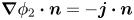 $\boldsymbol {\nabla }\phi _2\boldsymbol {\cdot }\boldsymbol {n}=-\boldsymbol {j}\boldsymbol {\cdot }\boldsymbol {n}$ at
  $\boldsymbol {x}$ on
  $S_{w}$, and
  $\phi _{2}$ vanishes as
  $\boldsymbol {x}\rightarrow \pm \infty$. Figures 2(b,d) show
  $\phi _2$ zoomed in at the aerofoils used in the present cases, with
  $AoA = 7.5^\circ$ and
  $10^\circ$, respectively. Through the same procedure as used for (2.12), one obtains
 $$\begin{gather} \int_{S_w}\bar{p}(\boldsymbol{n}\boldsymbol{\cdot} \boldsymbol{j}) \,{\rm d}A + \dfrac{1}{Re}\int_{S_w}(\boldsymbol{n}\times\bar{\boldsymbol{\omega}})\boldsymbol{\cdot} \boldsymbol{j} \,{\rm d}A\nonumber\\ {}=-\int_{V_R}\bar{\boldsymbol{u}}\times \bar{\boldsymbol{\omega}}\boldsymbol{\cdot} \boldsymbol{\nabla} \phi_2 \,{\rm d}V +\dfrac{1}{Re}\int_{S_w}\boldsymbol{n}\times\bar{\boldsymbol{\omega}}\boldsymbol{\cdot} (\boldsymbol{\nabla}\phi_2+\boldsymbol{j}) \,{\rm d}A +\int_{V_R}\boldsymbol{\nabla} \boldsymbol{\cdot} \boldsymbol{\tau}_{SGS} \boldsymbol{\cdot} \boldsymbol{\nabla} \phi_2 \,{\rm d}V \end{gather}$$
for the analysis of the contributions to the lift force. Using the same analogy as in (2.13), (2.14) leads to the equation for the instantaneous contributions to the total lift coefficient  $C_L$, expressed as
 \begin{equation} C_L = C_{L,V}+C_{L,S}+C_{L,SGS}, \end{equation}
where  $\bar {\boldsymbol {u}}\times \bar {\boldsymbol {\omega }}\boldsymbol {\cdot } \boldsymbol {\nabla } \phi _2$ are the volume lift elements,
 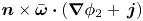 $\boldsymbol {n}\times \bar {\boldsymbol {\omega }}\boldsymbol {\cdot } (\boldsymbol {\nabla }\phi _2+\,\boldsymbol {j})$ are the surface lift elements, and
 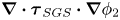 $\boldsymbol {\nabla } \boldsymbol {\cdot } \boldsymbol {\tau }_{SGS} \boldsymbol {\cdot } \boldsymbol {\nabla } \phi _2$ is the SGS contribution to lift.
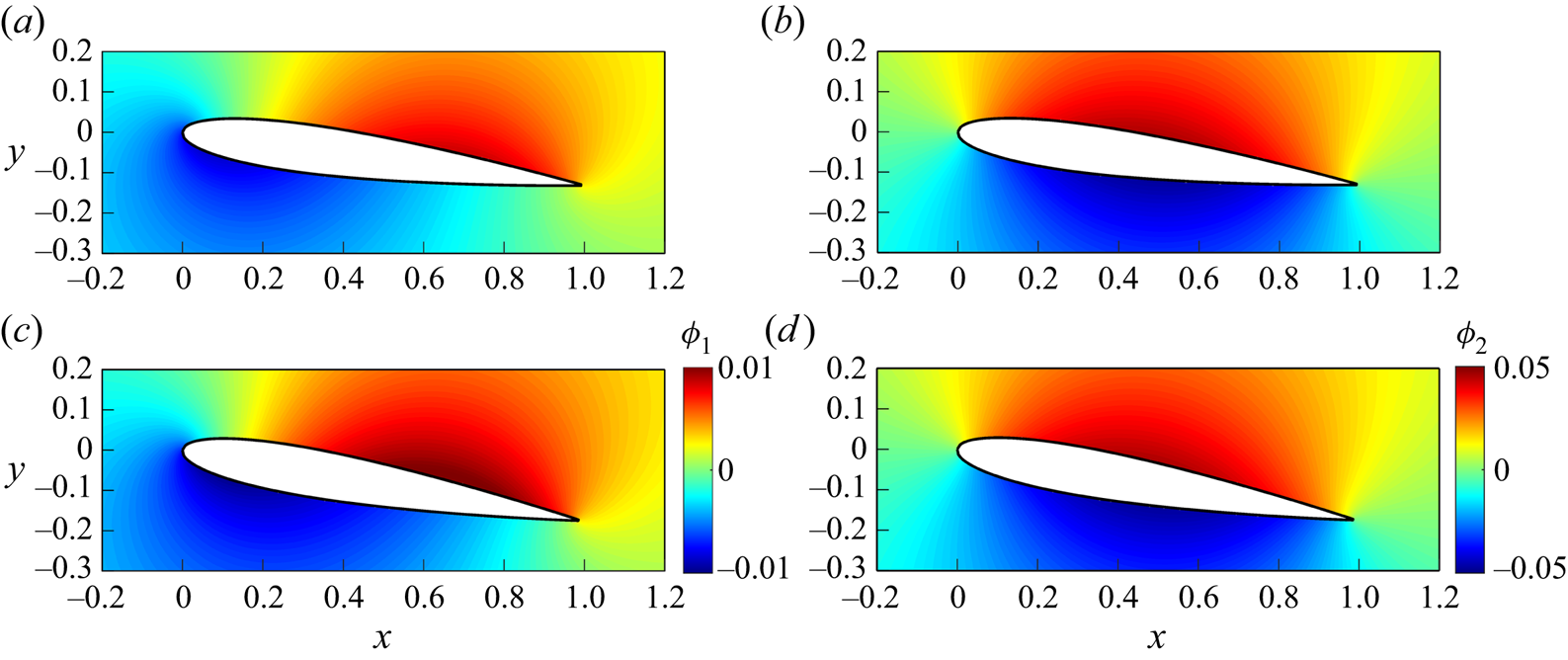
Figure 2. Auxiliary potentials  $\phi _1$ and
  $\phi _2$ zoomed in at the aerofoils in the present cases for (a) drag
  $\phi _1$ with
  $AoA = 7.5^\circ$, (b) lift
  $\phi _2$ with
  $AoA = 7.5^\circ$, (c) drag
  $\phi _1$ with
  $AoA = 10^\circ$, and (d) lift
  $\phi _2$ with
  $AoA = 10^\circ$.
3. Proper orthogonal decomposition
In this section, we outline the algorithm for computing the SPOD, and the data reconstruction using these SPOD modes. More detailed derivations and mathematical properties of SPOD can be found in Towne et al. (Reference Towne, Schmidt and Colonius2018), and the practical implementation of this method is provided by Schmidt & Towne (Reference Schmidt and Towne2019) and Schmidt & Colonius (Reference Schmidt and Colonius2020).
3.1. Spectral proper orthogonal decomposition
We first consider the instantaneous flow field  $\boldsymbol {q}(\boldsymbol {x},t)=(\bar {u},\bar {v},\bar {w})^{\rm T}$, which can be decomposed as
 \begin{equation} \boldsymbol{q}(\boldsymbol{x},t) = \tilde{\boldsymbol{q}}(\boldsymbol{x})+\boldsymbol{q}'(\boldsymbol{x},t), \end{equation}
where  $\tilde {\boldsymbol {q}}(\boldsymbol {x})$ is the temporal average of
  $\boldsymbol {q}(\boldsymbol {x},t)$, and
  $\boldsymbol {q}'(\boldsymbol {x},t)$ is its fluctuation. Let
  $\boldsymbol {q}'_{k}\in \mathbb {R}^{N_x}$ represent the fluctuating velocity vector at the
  $k$th time step, where
  $N_x$ is the number of discrete grid points times the number of variables (three in this study). Collecting all
  $\boldsymbol {q}'_{k}$ into a data matrix, we have
 \begin{equation} \boldsymbol{Q} = \begin{bmatrix} \vert & \vert & \vert & \vert & \vert \\ \boldsymbol{q}'_{1} & \boldsymbol{q}'_{2} & \boldsymbol{q}'_{3} & \cdots & \boldsymbol{q}'_{N_t}\\ \vert & \vert & \vert & \vert & \vert \end{bmatrix},\quad \boldsymbol{Q}\in\mathbb{R}^{N_{x}\times N_{t}}, \end{equation}
where  $N_{t}$ is the total step (total snapshots) of the numerical simulation. The aim of SPOD is to seek modes that are orthogonal in space–time inner product, which can be defined as
 \begin{equation} \langle\boldsymbol{U},\boldsymbol{V}\rangle_{\boldsymbol{x},t} = \int^{\infty}_{-\infty}\int_{\mathit{\varOmega}} \boldsymbol{U}^{*}(\boldsymbol{x},t)\,\boldsymbol{W}(\boldsymbol{x})\,\boldsymbol{V}(\boldsymbol{x},t)\,{\rm d}\kern0.06em \boldsymbol{x}\,{\rm d}t, \end{equation}
where  $\boldsymbol {U}$ and
  $\boldsymbol {V}$ are two arbitrary vectors, the asterisk denotes the conjugate transpose,
  $\mathit {\varOmega }$ is the spatial domain of interest, and
  $\boldsymbol {W}$ is a positive-definite Hermitian matrix. For statistically stationary data, the SPOD modes are obtained by solving the eigenvalue problem for the Fourier transformed two-point space–time correlation matrix (i.e. cross-spectral density):
 \begin{equation} \boldsymbol{S}(\boldsymbol{x},\boldsymbol{x}',f) = \int_{-\infty}^{\infty}\boldsymbol{C}(\boldsymbol{x},\boldsymbol{x}',\tau)\, {\rm e}^{-{\rm i}2{\rm \pi} f\tau}\,{\rm d}\tau, \end{equation}
where  $\tau = t-t'$, and
  $\boldsymbol {C}(\boldsymbol {x},\boldsymbol {x}',\tau )$ is the two-point space–time correlation tensor. Towne et al. (Reference Towne, Schmidt and Colonius2018) developed an algorithm to estimate
  $\boldsymbol {S}(\boldsymbol {x},\boldsymbol {x}',f)$ in (3.4) based on Welch's method (Welch Reference Welch1967). The data matrix
  $\boldsymbol {Q}$ in (3.2) is divided into
  $N_{blk}$ overlapping blocks with
  $N_{fft}$ snapshots in each of them, that is,
 \begin{equation} \boldsymbol{Q}^{(k)} = \begin{bmatrix} \vert & \vert & \vert & \vert \\ \boldsymbol{q}'^{(k)}_{1} & \boldsymbol{q}'^{(k)}_{2} & \cdots & \boldsymbol{q}'^{(k)}_{N_{fft}}\\ \vert & \vert & \vert & \vert \end{bmatrix},\quad k=1,2,\ldots,N_{blk}, \end{equation}
where superscript  $(k)$ denotes the
  $k$th block. Since blocks are overlapped by
  $n_{ovlp}$ snapshots, the
  $j$th column vector in the
  $k$th block
  $\boldsymbol {q}'^{(k)}_{j}$ corresponds to the
  $m$th column vector
  $\boldsymbol {q}'_{m}$ in the
  $\boldsymbol {Q}$ matrix (see (3.2)), where
 \begin{equation} m = j+(k-1)\times(N_{fft}-n_{ovlp})+1. \end{equation}
The discrete Fourier transform (DFT) is then applied to (3.5) to give
 \begin{equation} \hat{\boldsymbol{Q}}^{(k)} = \begin{bmatrix} \vert & \vert & \vert & \vert \\ \widehat{\boldsymbol{q}'}^{(k)}_{1} & \widehat{\boldsymbol{q}'}^{(k)}_{2} & \cdots & \widehat{\boldsymbol{q}'}^{(k)}_{N_{fft}}\\ \vert & \vert & \vert & \vert \end{bmatrix}, \end{equation}
where
 \begin{equation} \widehat{\boldsymbol{q}'}_{j}^{(k)} = \mathcal{F}\left\{w(\,j)\,\boldsymbol{q}'^{(k)}_{j}\right\}, \end{equation}
in which  $\mathcal {F}\{\,\cdot \,\}$ is DFT operator, and
  $w(\,j)$ is the window function to reduce spectral leakage. Here, we use the symmetric Hamming window function
 \begin{equation} w(\,j+1) = 0.54-0.46\cos\left(\dfrac{2{\rm \pi} j}{N_{fft}-1}\right), \quad \text{for } j=0,1,2,\ldots,N_{fft}-1. \end{equation}
The next step is to construct matrix  $\hat {\boldsymbol {Q}}_{i}$ containing the
  $i$th frequency (i.e.
  $i$th column) of each
  $\hat {\boldsymbol {Q}}^{(k)}$, such that
 \begin{equation} \hat{\boldsymbol{Q}}_{i} = \begin{bmatrix} \vert & \vert & \vert & \vert \\ \widehat{\boldsymbol{q}'}^{(1)}_{i} & \widehat{\boldsymbol{q}'}^{(2)}_{i} & \cdots & \widehat{\boldsymbol{q}'}^{(N_{blk})}_{i}\\ \vert & \vert & \vert & \vert \end{bmatrix},\quad \hat{\boldsymbol{Q}}_{i}\in\mathbb{R}^{N_{x}\times N_{blk}}, \end{equation}
and the cross spectral density  $\boldsymbol {S}_{i}$ at the
  $i$th frequency is given by
 \begin{equation} \boldsymbol{S}_{i} = \dfrac{1}{N_{blk}}\,\hat{\boldsymbol{Q}}_{i}\hat{\boldsymbol{Q}}^{*}_{i},\quad \boldsymbol{S}_{i}\in\mathbb{R}^{N_{x}\times N_{x}}, \end{equation}
which leads to the eigenvalue problem
 \begin{equation} \boldsymbol{S}_{i}\boldsymbol{W}\boldsymbol{\varPhi}_{i} = \boldsymbol{\varPhi}_{i}\boldsymbol{\varLambda}_{i}, \end{equation}
where  $\boldsymbol {\varPhi }_{i} = [\boldsymbol {\phi }^{(1)}_{i},\boldsymbol {\phi }^{(2)}_{i},\ldots,\boldsymbol {\phi }^{(N_{blk})}_{i}]$ are the SPOD modes (eigenvectors) at the
  $i$th frequency, and
  $\boldsymbol {\varLambda }_{i} = \mbox {diag}(\lambda ^{(1)}_{i},\lambda ^{(2)}_{i},\ldots,\lambda ^{(N_{blk})}_{i} )$ is the eigenvalue corresponding to the SPOD mode energy, where by convention,
  $\lambda ^{(1)}_{i}\geq \lambda ^{(2)}_{i}\geq \cdots \geq \lambda ^{(N_{blk})}_{i}$. It should be noted that different choices of
  $\boldsymbol {W}$ affect the coherent structures obtained from (3.12) (Schmidt & Colonius Reference Schmidt and Colonius2020). In this study, we specified the weighted matrix
  $\boldsymbol {W}$ as
 \begin{equation} \boldsymbol{W} = \int_{V_{R}} \begin{bmatrix} 1 & & \\ & 1 & \\ & & 1 \end{bmatrix} \,{\rm d}V, \end{equation}
to extract the turbulence kinematic energy from the current dataset  $\boldsymbol {Q}$. However, in practice, the total number of data points
  $N_{x}$ is typically much larger than the number of blocks
  $N_{blk}$. Hence, instead of using (3.12), it is more economical to obtain SPOD modes
  $\boldsymbol {\varPhi }_{i}$ by the analogous eigenvalue problem (Sirovich Reference Sirovich1987)
 \begin{equation} \dfrac{1}{N_{blk}}\,\hat{\boldsymbol{Q}}^{*}_{i}\boldsymbol{W}\hat{\boldsymbol{Q}}_{i}\boldsymbol{\varPsi}_{i} = \boldsymbol{\varPsi}_{i}\boldsymbol{\varLambda}_{i}, \quad \hat{\boldsymbol{Q}}^{*}_{i}\boldsymbol{W}\hat{\boldsymbol{Q}}_{i} \in \mathbb{R}^{N_{blk}\times N_{blk}}, \end{equation}
and the SPOD modes  $\boldsymbol {\varPhi }_{i}$ can be evaluated in terms of
  $\boldsymbol {\varPsi }_{i}$ as
 \begin{equation} \boldsymbol{\varPhi}_{i} = \dfrac{1}{\sqrt{N_{blk}}}\,\hat{\boldsymbol{Q}}_{i}\boldsymbol{\varPsi}_{i}\boldsymbol{\varLambda}^{-{1}/{2}}_{i}. \end{equation}
3.2. Low-rank data reconstruction
Due to the optimality of SPOD modes, the best approximation to the current data matrix  $\boldsymbol {Q}$ is truncated expansion with the first
  $n$ set of the SPOD basis (Schmidt & Colonius Reference Schmidt and Colonius2020). The objective of this study is to examine the actual impact of coherent structures on aerodynamic forces at a specific moment in time. To achieve this, it is crucial to determine the precise values of drag and lift forces induced by each SPOD mode at that particular time instant. While applying the vorticity force representation to each SPOD mode captures the drag/lift coefficients oscillating at a single frequency, the actual magnitude in time remains unknown. Consequently, we are unable to determine which coherent structure predominantly influences the overall behaviours of the original
  $C_{D/L,V}$. In this regard, the present method involves accurately converting the flow quantities associated with SPOD modes
  $\boldsymbol {\varPhi }_{i}$, including their magnitudes represented by expansion coefficients, from the frequency domain to the time domain using a reconstruction technique. Here, we adopted the low-rank data reconstruction technique proposed by Nekkanti & Schmidt (Reference Nekkanti and Schmidt2021), referred to as ‘frequency domain reconstruction’. By inverting the SPOD process in the previous subsection, we have the original realizations of the Fourier transform at each frequency:
 \begin{equation} \hat{\boldsymbol{Q}}_{i} = \boldsymbol{\varPhi}_{i}\boldsymbol{A}_{i}, \end{equation}
where  $\boldsymbol {A}_{i}$ is the expansion coefficient of the
  $i$th frequency,
 \begin{equation} \boldsymbol{A}_{i} = \sqrt{N_{blk}}\,\boldsymbol{\varLambda}^{{1}/{2}}_{i}\boldsymbol{\varPsi}^{*}_{i} = \boldsymbol{\varPhi}^{*}_{i}\boldsymbol{W}\hat{\boldsymbol{Q}}_{i},\quad \boldsymbol{A}_{i} =\begin{bmatrix} a_{11} & a_{12} & \cdots & a_{1N_{blk}}\\ a_{21} & a_{22} & \cdots & a_{2N_{blk}}\\ \vdots & \vdots & \ddots & \vdots \\ a_{N_{blk}1} & a_{N_{blk}2} & \cdots & a_{N_{blk}N_{blk}} \end{bmatrix}_{i}. \end{equation}
The Fourier-transformed data of the  $k$th block can be reassembled by
 \begin{equation} \hat{\boldsymbol{Q}}^{(k)} = \left[\left(\sum_{m}a_{mk}\boldsymbol{\phi}^{(m)}\right)_{i=1},\left(\sum_{m}a_{mk}\boldsymbol{\phi}^{(m)}\right)_{i=2},\ldots,\left(\sum_{m}a_{mk}\boldsymbol{\phi}^{(m)}\right)_{i=N_{fft}} \right], \end{equation}
where  $m$ denotes the first
  $m$ SPOD modes summation. Applying the inverse Fourier transform, the data matrix in the time domain is expressed as
 \begin{equation} \boldsymbol{q}'^{(k)}_{i} = \dfrac{1}{w(i)}\,\mathcal{F}^{-1}\left\{\left(\sum_{m} a_{mk}\boldsymbol{\phi}^{(m)}\right)_{i}\right\}. \end{equation}
Finally, the window-weighted average is adopted to the  $i$th step, which is overlapped in two adjacent blocks (
 $k$ and
  $k+1$):
 \begin{equation} \boldsymbol{q}'_{i} = \dfrac{\boldsymbol{q}'^{(k)}_{j}\,w(\,j)+\boldsymbol{q}'^{(k+1)}_{j-n_{ovlp}}\,w\left(\left\vert \,j-n_{ovlp} \right\vert\right)}{w(\,j)+w\left(\left\vert \,j-n_{ovlp}\right\vert\right)}, \end{equation}
where  $j=i-(k-1)(N_{fft}-n_{ovlp})$. Although Nekkanti & Schmidt (Reference Nekkanti and Schmidt2021) have proposed another technique called ‘time domain reconstruction’ and demonstrated superior performance compared to the aforementioned method, we find the frequency domain reconstruction to be a more straightforward approach for implementing the complete algorithm. Hence, in the present study, all of the reconstructed results in the following sections are conducted by the above procedures.
Based on the above procedures, we can expand the flow velocity as
 \begin{equation} \bar{\boldsymbol{u}} = {\bar{\boldsymbol{u}}}^{(0)} + \sum_{m=1}^{N_{blk}} \bar{\boldsymbol{u}}'^{(m)}, \end{equation}
where  $\bar {\boldsymbol {u}}^{(0)}$ is the zeroth mode obtained from temporal average of
  $\bar {\boldsymbol {u}}$, and
  $\bar {\boldsymbol {u}}'^{(m)}$ denotes the
  $m$th mode velocity reconstructed by SPOD basis. This allows us to reduce the complexity and identify the coherent structures within turbulent flows. Moreover, the effect of these coherent structures on drag and lift coefficients can be quantified using vorticity force analysis (see (2.12) and (2.14)). For example, substituting (3.21) into the first term (volumetric vorticity force) of (2.13), we have
 \begin{equation} C_{D,V} = C^{(0)}_{D,V}+\sum^{N_{blk}}_{m = 1} C^{(m)}_{D,V}, \end{equation}
where
 \begin{equation} \left. \begin{gathered} C^{(0)}_{D,V} = C^{00}_{D,V},\\ C^{(1)}_{D,V} = C^{10}_{D,V}+C^{11}_{D,V},\\ C^{(2)}_{D,V} = C^{20}_{D,V}+C^{21}_{D,V}+C^{22}_{D,V},\\ C^{(3)}_{D,V} = C^{30}_{D,V}+C^{31}_{D,V}+C^{32}_{D,V}+C^{33}_{D,V},\\ \vdots\\ C^{(m)}_{D,V} = C^{m0}_{D,V}+C^{m1}_{D,V}+C^{m2}_{D,V}+\cdots +C^{mm-1}_{D,V}+C^{mm}_{D,V}, \end{gathered} \right\} \end{equation}
is the  $m$th mode contribution to the total
  $C_{D,V}$, and
 \begin{equation} C^{mn}_{D,V} = \begin{cases} \displaystyle\int_{V_{R}}\bar{\boldsymbol{u}}'^{(m)}\times\bar{\boldsymbol{\omega}}'^{(n)}\boldsymbol{\cdot}\boldsymbol{\nabla}\phi_{1}\,{\rm d}V & \text{for }m=n,\\ \displaystyle\int_{V_{R}}\left(\bar{\boldsymbol{u}}'^{(m)}\times\bar{\boldsymbol{\omega}}'^{(n)}+\bar{\boldsymbol{u}}'^{(n)}\times\bar{\boldsymbol{\omega}}'^{(m)}\right)\boldsymbol{\cdot}\boldsymbol{\nabla}\phi_{1}\,{\rm d}V & \text{for }m\neq n,\\ \end{cases} \end{equation}
is the volumetric vorticity force caused by the interaction between the  $m$th and
  $n$th modes. As shown in (3.23) and (3.24),
  $C^{(m)}_{D,V}$ includes effects of zeroth mode/
 $m$th mode,
  $m$th mode/
 $k$th mode (
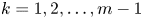 $k=1,2,\ldots,m-1$) and
  $m$th mode/
 $m$th mode interactions, respectively. With these, the importance of each coherent structure can be evaluated quantitatively and provide insight into the physical interpretation of the complex turbulent flows via mode interaction. Similarly,
  $C_{L,V}$ can be decomposed into
 \begin{equation} C_{L,V} = C^{(0)}_{L,V}+\sum^{N_{blk}}_{m = 1} C^{(m)}_{L,V}, \end{equation}
4. Numerical modelling
Solutions of the Navier–Stokes equations are obtained by the commercial software ANSYS FLUENT (Fluent Reference Fluent2013), which discretizes the governing equations using the finite-volume method, and uses a pressure implicit splitting operator (Issa Reference Issa1986) to solve the incompressible flow field. The spatial discretization is second-order accurate, while the time marching scheme is second-order implicit. Transport of momentum is solved using QUICK (Leonard Reference Leonard1979). Here, we use LES, in which the dynamic Smagorinsky–Lilly model (Lilly Reference Lilly1992) is used to obtain the SGS stresses.
As shown in figure 3, an NACA0012 aerofoil with length  $L$ is placed at the central region of the domain, in which C-type grids are used. In the literature, a constant trade-off exists when selecting the domain size, balancing the need to accurately capture flow phenomena with the goal of minimizing computational costs. To this end, Jones et al. (Reference Jones, Sandberg and Sandham2008) carried out systematic investigations to determine the optimal domain size and grid resolutions for DNS of LSB on an NACA0012 aerofoil at
  $Re=50\,000$ and
  $AoA=5^{\circ }$. Based on their findings, they suggested that a domain length in the
  $x$-direction ranging from approximately
  $11.3L$ to
  $13.3L$, and a domain height in the
  $y$-direction of approximately
  $10L$, are suitable for accurately simulating such flow conditions. In addition, they also demonstrated that domain width
  $0.2L$ in the
  $z$-direction is sufficient to capture the movements of small-scale eddies in the spanwise direction. Therefore, in this study the domain dimension is
  $21L$ in the
  $x$-direction,
  $20 L$ in the
  $y$-direction – which is slightly larger than that suggested by Jones et al. (Reference Jones, Sandberg and Sandham2008) – and
  $0.2L$ in the
  $z$-direction. This choice also aligns with recommendations from Liu & Xiao (Reference Liu and Xiao2020), Kojima et al. (Reference Kojima, Nonomura, Oyama and Fujii2012) and Yeh & Taira (Reference Yeh and Taira2019) for cases involving
  $Re\sim O(10^{4})$ and low
  $AoA$, as well as with guidance from Turner & Kim (Reference Turner and Kim2022) and Rodriguez et al. (Reference Rodriguez, Lehmkuhl, Borrell and Oliva2013) in scenarios with full-stall conditions, where domain size
  $0.1L$ was utilized. However, we observed that in the present case with the larger
  $AoA$ (
 $10^\circ$), the two-point correlation of the streamwise velocity does not approach zero at the half-width of the domain. It is worth noting that due to computational resource limitations, we restricted the spanwise dimension to
  $0.2L$, but a larger dimension may be required for future studies. With
  $96$ grid cells in the
  $z$-direction, the total number of grid cells is around
  $7\,200\,000$, which varies slightly between cases depending on the configuration (i.e. different angles of attack). Figure 4 presents a two-dimensional view of the total grid configuration on the
  $xy$-plane (figure 4a) and a zoom-in figure to show the compressed grid cells on the surface of the aerofoil (figure 4b). Simulations begin with a background uniform velocity
  $U_{\infty }$ in the
  $x$-direction such that the Reynolds number is
 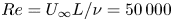 $Re = U_{\infty } L/\nu = 50\,000$, where
  $L=0.1\ \textrm {m}$ is the chord length of the aerofoil, and
 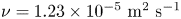 $\nu =1.23\times 10^{-5}\ \textrm {m}^2\ \textrm {s}^{-1}$ is the kinematic viscosity. In the present simulations, grids are always compressed on the near-wall region of the aerofoil such that
 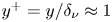 $y^+ = y/\delta _\nu \approx 1$ at the bottom-most grid point on the aerofoil. This can be confirmed by outputting the distribution of
  $y^+$ at the bottom-most grid points on the aerofoil calculated based on the instantaneous wall shear stress, as shown in figure 5, where we show that typical values at a representative instant of time range mostly from
  $0.5$ to
  $2$, while values greater than
  $3$ are found at just few points. Additionally, we find that
  $13 \leq x^+ \leq 22$ and
  $8 \leq z^+ \leq 14$. While these values slightly exceed the DNS mesh size recommendations proposed by Georgiadis, Rizzetta & Fureby (Reference Georgiadis, Rizzetta and Fureby2010) (
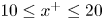 $10 \leq x^+ \leq 20$ and
  $5 \leq z^+ \leq 10$), they remain suitable for achieving the resolution necessary for the LES.
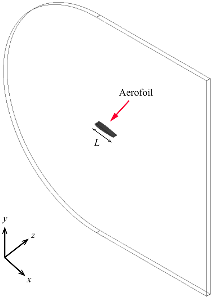
Figure 3. Schematic showing the domain configuration of the present simulations ( $AoA=7.5^{\circ }$), where
  $L=0.1$ m is the chord length of the aerofoil.
Figure 4. (a) Computational grid on the  $xy$-plane in the case with
  $AoA = 7.5^\circ$, and (b) its zoomed-in image around the aerofoil.
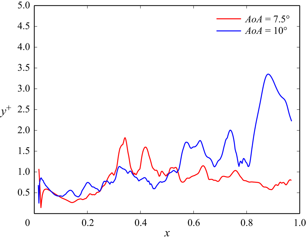
Figure 5. An example of instantaneous distributions of the values of  $y^+$ of the bottom-most grid cells at a time instant in cases with
  $AoA = 7.5^\circ$ (red) and
  $AoA = 10^\circ$ (blue).
To examine the dependence of the numerical results on grid resolutions, we also performed simulations using coarser ( $5\,400\,000$ cells) and finer (
 $9\,600\,000$ cells) grid resolutions than that of the present study (referred to as the medium grid resolution). While progressing from a coarser to a medium mesh, we first enhanced the resolution along the streamwise direction on the aerofoil's surface. Subsequently, we refined the resolution vertically at the same position, exceeding the medium mesh resolution by one and a half times. Figure 6 presents the mean pressure coefficient
  $C_p$ obtained from the present numerical simulations (
 $AoA=7.5^{\circ }$) along with the LES results in Lehmkuhl et al. (Reference Lehmkuhl, Rodríguez, Baez, Oliva and Pérez-Segarra2013) using the QR eddy viscosity model in the case with
  $AoA = 8^\circ$. Lehmkuhl et al. (Reference Lehmkuhl, Rodríguez, Baez, Oliva and Pérez-Segarra2013) show that the pressure drops at two locations (see the grey solid line in figure 6): one at the leading edge (
 $x \approx 0$), and the other at a point close to the centre of the chord (
 $x \approx 0.3$). It is apparent that the coarse grid (see the black dash-dotted line) fails to capture the second point of pressure drop. On the other hand, the medium resolution (see the black solid line) shows that at both of these points, the profile of
  $C_{p}$ slightly underestimates/overestimates the sudden decrease of the pressure. Despite this, fair agreement between the present result and results from the LES by Lehmkuhl et al. (Reference Lehmkuhl, Rodríguez, Baez, Oliva and Pérez-Segarra2013) can be seen. In contrast to the variations observed between cases of coarse and medium grid resolutions, the distinction between cases of medium and fine grid resolutions (see the black dashed line) appears to be insignificant. Thus we can affirm confidently that minor deviations in outcomes do not stem solely from variations in mesh configurations, indicating that grid convergence can be achieved at the medium grid resolution. Therefore, in this study, we use the medium grid resolution to obtain the numerical results.
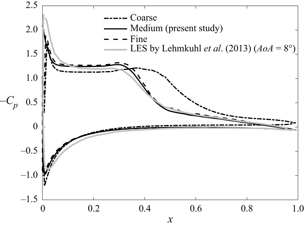
Figure 6. Distributions of the pressure coefficient ( $C_p$) on the surface of the NACA0012 aerofoil in the case with
  $AoA = 7.5^\circ$ obtained from the present simulation with coarse (black dash-dotted line), medium (black solid line) and fine (black dashed line) grid resolutions, and the LES by Lehmkuhl et al. (Reference Lehmkuhl, Rodríguez, Baez, Oliva and Pérez-Segarra2013) using the QR eddy-viscosity model (grey solid line).
As for the SPOD procedure, LES data consist of  $1000$ snapshots in each angle of attack case, and the SPOD modes are computed for blocks containing
  $N_{fft}=64$ snapshots with
  $50\,\%$ overlap (to minimize the variance of the spectral estimate), resulting in a total number of blocks
  $N_{blk}=30$. It should be noted that selecting appropriate values for
  $N_{fft}$ and
  $N_{blk}$ is considered state of the art in SPOD research. During our simulation period, we discovered that applying SPOD with
  $N_{fft}=64$ and
  $N_{fft}=128$ per block yielded nearly identical results for the first two modes, and the first three frequencies obtained from the
  $N_{fft}=64$ case are enough to capture the fundamental frequency of the wake in our simulations, which will be discussed later. Consequently, to retain simplicity, we used
  $N_{fft}=64$ per block to construct the SPOD modes for the subsequent analyses. Furthermore, the SPOD mode convergence for the current set-up is also checked by using the method proposed by Abreu, Cavalieri & Wolf (Reference Abreu, Cavalieri and Wolf2017), and the details are shown in Appendix A.
5. Flow fields and total vorticity forces
Figure 7 presents the mean streamwise velocity  $\tilde {\bar {u}}$, along with the streamlines in two cases of different
  $AoA$. Here, the mean velocity is obtained by applying the spatial and temporal averages to the velocity field. Flow separation behind the leading edge can be found in both cases, but in the case with
  $AoA = 7.5^\circ$, figure 7(a) shows that the separated flow reattaches to the aerofoil surface at
  $x \approx 0.3$, forming a bubble-like flow structure in the mean field, which is known as the laminar separation bubble (LSB). When
  $AoA$ increases, as shown in figure 7(b), the separated flow no longer reattaches. In the cases with the larger
  $AoA$, as shown in figure 7(b), the extension of the separation region to the trailing edge results in a strong shear layer behind the trailing edge. This leads to the formation of the trailing-edge vortex (TEV), which is absent in the low-
 $AoA$ cases. In the present study, under the same
  $Re$, the reattachment, detachment and TEV characterize three distinct flow regimes from low to high values of
  $AoA$.
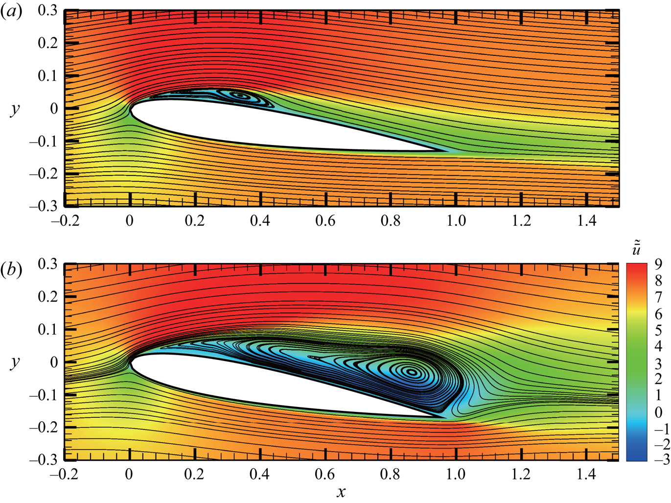
Figure 7. The mean streamwise velocity along with the streamlines of the mean flow field in cases with (a)  $AoA = 7.5^\circ$, and (b)
  $AoA = 10^\circ$.
In addition to the mean flow field, root-mean-square (r.m.s.) of fluctuating streamwise velocity  $\mbox {r.m.s.}(u')$ at the central slice in the
  $z$-direction in cases with
  $AoA=7.5^{\circ }$ and
  $AoA=10^{\circ }$ are plotted in figure 8. It can be seen from figure 8(a) that at
  $AoA=7.5^{\circ }$,
  $\mbox {r.m.s.}(u')$ is concentrated within the LSB (see figure 7a). On the other hand, without flow reattachment, values of
  $\mbox {r.m.s.}(u')$ in the case with
  $AoA=10^{\circ }$ are higher along the shear layer and near the trailing edge, as shown in figure 8(b). Next, fluctuation quantities associated with vortex shedding frequency (Roshko Reference Roshko1961; Huang & Lin Reference Huang and Lin2000) are further examined via the power spectra of vertical velocity. At
  $AoA=7.5^{\circ }$, vertical velocity fluctuation is measured at five points (
 $P1$–
$P1$– $P5$) positioned at distances 5–8 grid units from the upper surface. Furthermore, the last point,
  $P6$, is probed in the wake region. In the case with
  $AoA=10^{\circ }$, points
  $P1$–
$P1$– $P5$ are chosen specifically along the shear layer depicted in figure 7(b), while
  $P6$ is located at the wake region. Figures 9(a,b) present the power spectra of the vertical velocity sampled at six points along the upper side of the aerofoil, as shown by
  $P1$–
$P1$– $P5$ in figures 9(c,d), in cases with
  $AoA = 7.5^\circ$ and
  $10^\circ$, respectively. In general, the spectra with slope
  $-5/3$ (marked by the dashed line), i.e. the inertial subrange, can be found for both
  $AoA$ values, particularly near the trailing edge, i.e. points
  $P5$ and
  $P6$. At the point closest to the leading edge (i.e.
  $P1$), a high-frequency peak (
 $St \approx 11$) can be found in both
  $AoA$ cases. These peaks correspond to shear instabilities, which disappear as the flow moves downstream and transforms to turbulence. Another important feature is in the large
  $AoA$ case is the presence of a low-energy peak at
  $St \approx 11$ at the station
  $P6$, as shown in figure 9(b). This is the fundamental frequency that corresponds to the wake, which plays a crucial role in aerodynamic forces exerted on the aerofoil, as discussed in the following sections. It is worthwhile mentioning that the power spectra shown in figure 9(b) are very similar to those obtained from the DNS results with slightly smaller
  $AoA$ (
 $=9.25^\circ$) in Rodriguez et al. (Reference Rodriguez, Lehmkuhl, Borrell and Oliva2013). Because the flow reattachment suppresses the wake, the fundamental frequency is not found in the smaller
  $AoA$ case (see figure 9a).
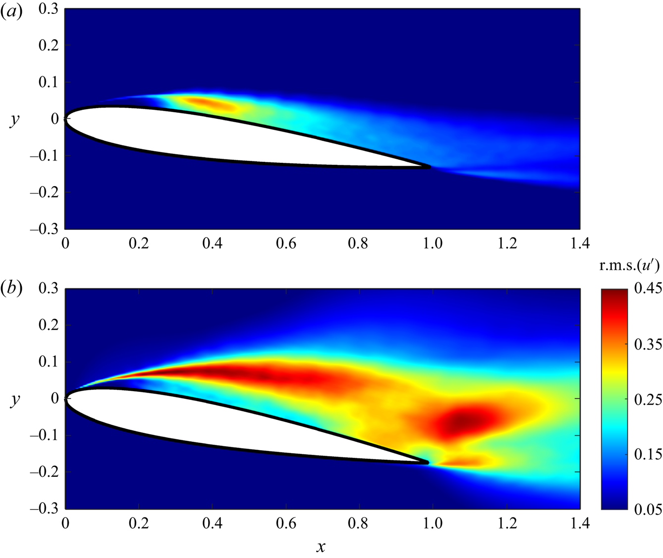
Figure 8. Root-mean-square (r.m.s.) of fluctuating streamwise velocity  $u'=\bar {u}-\tilde {\bar {u}}$ at the central slice in the
  $z$-direction in cases with (a)
  $AoA = 7.5^\circ$, and (b)
  $AoA = 10^\circ$.
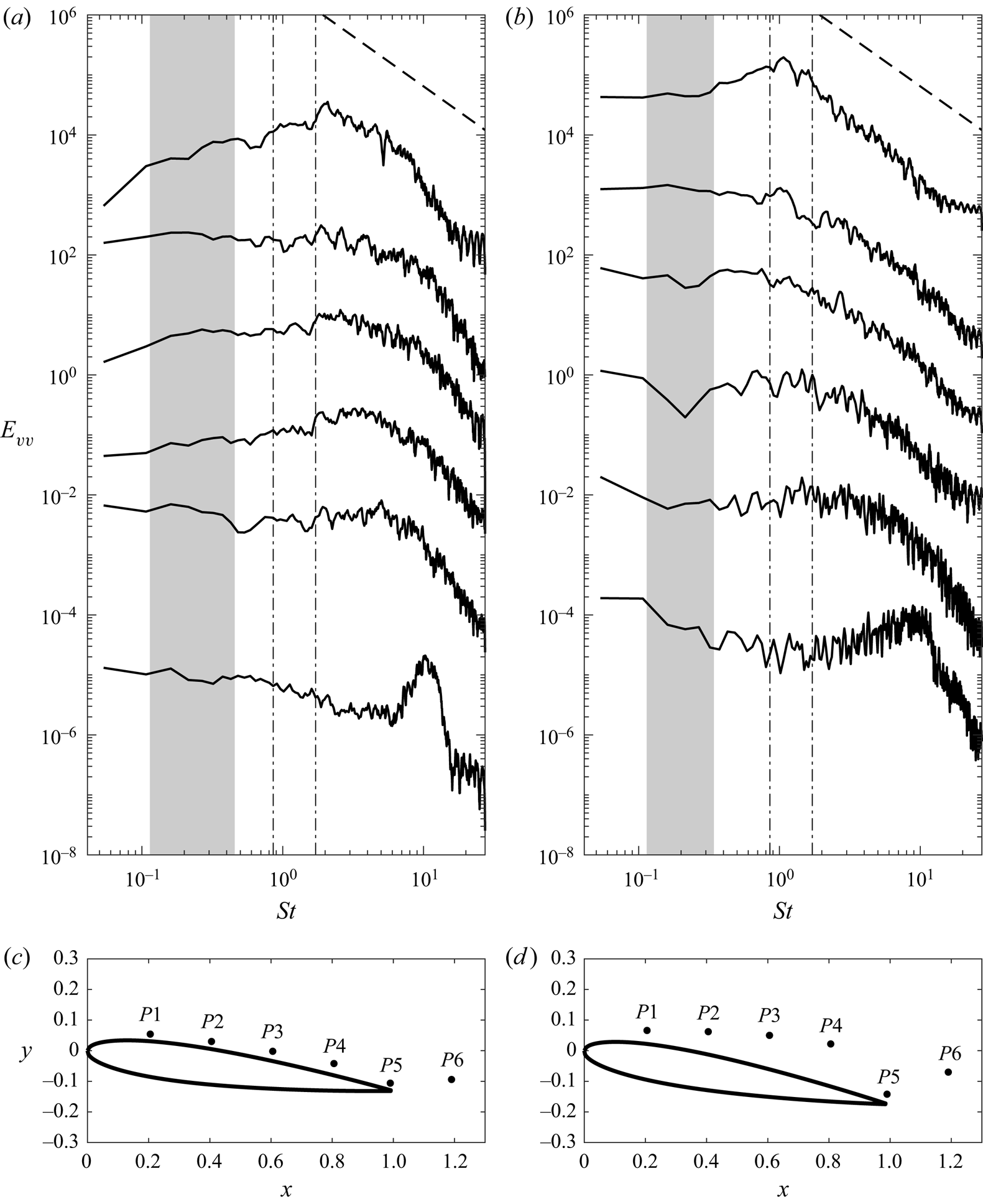
Figure 9. Power spectra of the vertical velocity in the cases with (a)  $AoA = 7.5^\circ$, and (b)
  $AoA = 10^\circ$. From top to bottom, spectra in (a,b) correspond to points
  $P6$,
$P6$,  $P5$,
$P5$,  $P4$,
$P4$,  $P3$,
$P3$,  $P2$ and
  $P1$ in (c,d), respectively. The dashed lines represent slope
  $-5/3$. The grey areas highlight the low-frequency range of the zeroth mode, while the dash-dotted lines in each case indicate the first (left-hand line) and second (right-hand line) frequencies in the present SPOD analysis.
Figure 10 presents time series of the total drag and lift coefficients, and all the contributions from the vorticity force analysis according to (2.13) and (2.15), for the present cases, where we also indicate the averaged values  $\tilde {C}_D$ and
  $\tilde {C}_L$. As summarized in table 1, values of
  $\tilde {C}_D$ and
  $\tilde {C}_L$ with different
  $AoA$ in the present study are close to those predicted by Musial & Cromack (Reference Musial and Cromack1988) based on the experimental data of Sheldahl & Klimas (Reference Sheldahl and Klimas1981) and Miley (Reference Miley1982). The magnitudes of the surface contribution (
 $C_{D, S}$ or
  $C_{L, S}$) in all cases are similar, while the total drag and lift are increasingly dominated by the volumetric term (
 $C_{D,V}$ or
  $C_{L,V}$), with increasing
  $AoA$. Except for the drag in the case with
  $AoA = 7.5^\circ$, where
  $C_{D,S}$ is about one-fifth of the volume contribution (
 $C_{D,V}$),
  $C_{D, V}$ is typically greater than all the other terms by more than one order of magnitude. Also, because the small grid size in the near field results in small values of the eddy viscosity in the present SGS model (i.e. eddy viscosity
  $<0.1\nu$), the SGS contributions (
 $C_{D,SGS}$ and
  $C_{L,SGS}$) are negligible (
 $< 1\,\%\,C_{D,V}$ or
  $< 1\,\%\,C_{L, V}$) compared with the others in all of the present cases, and are not plotted in figure 10. The dominance of the volumetric terms indicates that in such flow regimes, the coherent structures, particularly the vortices, play crucial roles in forces exerted on the aerofoil. In what follows, our discussion is on only the volumetric terms. Figure 11 is utilized to demonstrate visually how the generation of drag force occurs through the interaction between velocity and vorticity fields in the case with
  $AoA=10^{\circ }$. The dominant contributing factor to the volume drag element can be observed from figures 11(a,b), where it is typically the outcome of multiplying the streamwise velocity with the spanwise vorticity. Figure 11(c) illustrates that the streamwise vorticity maintains a positive value within the shear layer, while negative values are concentrated beneath it. This leads to a negative distribution of vorticity across the shear layer, as depicted in figure 11(d). Upon combining
  $\bar {u}$,
  $\bar {\omega }_{z}$ and
  ${\partial \phi _{1}}/{\partial y}$, which are negative within the region of interest (see figure 11e), it can be concluded that the drag force is attributed primarily to the positive distribution of the shear layer, as demonstrated in figure 11(b).
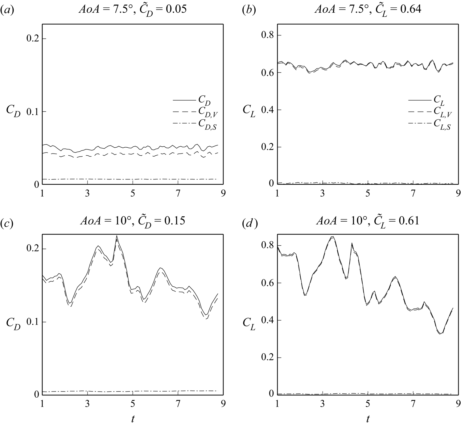
Figure 10. Time series of (a,c) drag and (b,d) lift coefficients, with their mean values, denoted with tildes, and the volumetric ( $C_{D,V}$ and
  $C_{L, V}$) and surface (
 $C_{D,S}$ and
  $C_{L, S}$) vorticity force contributions in cases with (a,b)
  $AoA = 7.5^\circ$, and (c,d)
  $AoA = 10^\circ$.
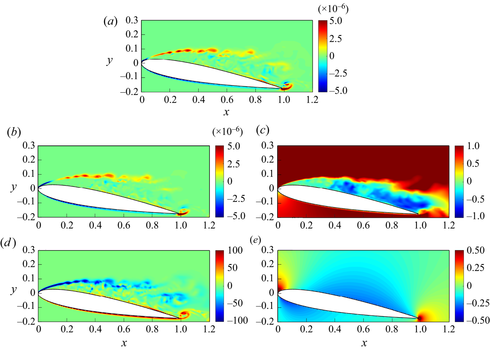
Figure 11. Snapshots of (a) volume drag element  $-(\bar {\boldsymbol {u}}\times \bar {\boldsymbol {\omega }})\boldsymbol {\cdot }\boldsymbol {\nabla }\phi _{1}$, (b) one of its components
  $\bar {u}\times \bar {\omega }_{z}\times {\partial \phi _{1}}/{\partial y}$, (c)
  $\bar {u}$ (d)
  $\bar {\omega }_{z}$ and (e)
  ${\partial \phi _{1}}/{\partial y}$, at the central slice in the
  $z$-direction at
  $t=3.83$ in the case with
  $AoA=10^{\circ }$.
Table 1. Comparisons of temporal average of drag ( $\tilde {C}_{D}$) and lift (
 $\tilde {C}_{L}$) coefficients between existing data and the present cases.
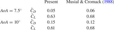
6. Effect of SPOD modes on aerodynamic forces
Figure 12 displays the eigenvalues of the SPOD modes as a function of the Strouhal number ( $St=fU_{\infty }/L$) for different
  $AoA$. It can be seen that the relative importance in terms of energy decreases with increasing mode.

Figure 12. Eigenvalues  $\lambda _{m}$ of the
  $m$th SPOD mode as a function of Strouhal number (
 $St$) in the cases with (a)
  $AoA=7.5^{\circ }$, and (b)
  $AoA=10^{\circ }$.
To examine the convergence to the total drag of the mode cumulation from  $C^{00}_{D,V}$ to
  $C^{MN}_{D,V}$, we introduce a force convergence index. Taking drag as an example, the force convergence index is defined as
 \begin{equation} R^{M}_{D} = \dfrac{\displaystyle\sum_{j=1}^{N_T}\left\vert\sum_{m=0}^{M}C^{(m)}_{D,V} -C^{(0)}_{D,V}\right\vert+N_TC^{(0)}_{D,V}}{\displaystyle\sum_{j=1}^{N_T}\left\vert C_{D,V}-C^{(0)}_{D,V}\right\vert+N_TC^{(0)}_{D,V}}\times 100\,\%. \end{equation}
Based on the vorticity force theory, (6.1) indicates how well the the drag/lift of the bulk flow can be approximated by the mode cumulation covered by the  $M$th mode. In the same analogy, we define the force convergence index for lift, denoted as
  $R^{M}_{L}$. Figure 13 shows
  $R^{M}_{D,V}$ and
  $R^{M}_{D,L}$ against
  $M$ in cases with
  $AoA = 7.5^\circ$ and
  $10^\circ$. Because of the relatively small time variations of both
  $C_{D,V}$ and
  $C_{L,V}$ in the low
  $AoA$ case due to the flow reattachment, the magnitude of total force can be well approximated by considering only the mean flow field (i.e. zeroth mode) for both drag (
 $R^{00}_{D} = 89.9\,\%$) and lift (
 $R^{00}_{L} = 95.6\,\%$). As shown in figure 13(a), convergence for drag and lift coefficients becomes fairly slow after the second mode is added. Different from those with
  $AoA=7.5^{\circ }$, the zeroth mode in the case with
  $AoA = 10^\circ$ has relative lower percentage of the total drag and lift contributions. The rapid convergence is reached (
 $97\,\%$ for drag and
  $99\,\%$ for lift) after taking
  $C^{(2)}_{D,V}$ and
  $C^{(2)}_{L,V}$ into account. Next, to examine the force convergence due to the contribution arising from the interactions between modes, we introduce force convergence indices that consider mode–mode interactions. For drag, this is expressed as
 \begin{equation} \tilde{R}^{MN}_{D} =
\dfrac{\displaystyle\sum_{j=1}^{N_T}\left\vert\sum_{m=0}^{M-1}C^{(m)}_{D,V}+\sum^{N
\le M}_{n=0}C^{Mn}_{D,V}
-C^{(0)}_{D,V}\right\vert+N_TC^{(0)}_{D,V}}{\displaystyle\sum_{j=1}^{N_T}\left\vert
C_{D,V}-C^{(0)}_{D,V}\right\vert+N_TC^{(0)}_{D,V}}\times
100\,\%,
\end{equation}
\begin{equation} \tilde{R}^{MN}_{D} =
\dfrac{\displaystyle\sum_{j=1}^{N_T}\left\vert\sum_{m=0}^{M-1}C^{(m)}_{D,V}+\sum^{N
\le M}_{n=0}C^{Mn}_{D,V}
-C^{(0)}_{D,V}\right\vert+N_TC^{(0)}_{D,V}}{\displaystyle\sum_{j=1}^{N_T}\left\vert
C_{D,V}-C^{(0)}_{D,V}\right\vert+N_TC^{(0)}_{D,V}}\times
100\,\%,
\end{equation}
and  $\tilde {R}^{MN}_{L}$ is defined for lift by analogy. Both
  $R^{MN}_{D,V}$ and
  $R^{MN}_{D,L}$ for the first two non-zero modes (
 $0 < M$,
  $N \le 2$) along with the zeroth mode (
 $M,N = 0$) are summarized in table 2. Overall, this shows that for non-zero modes, only their interactions with the zeroth mode (i.e.
  $MN = 10$ and
  $20$) dominate the force contribution, while the contributions of mode–mode interactions are typically negligible, as
 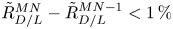 $\tilde {R}^{MN}_{D/L}-\tilde {R}^{MN-1}_{D/L} < 1\,\%$. Moreover, while the effect of the second mode is relatively minor in the small
  $AoA$ case, it becomes much more important in the large
  $AoA$ case. To make the discussion more concise, in what follows, we consider only the mode contributions that are greater than
  $1\,\%$. That is, we examine the force contribution due to the interactions of the zeroth mode and mode
  $1$ in the case with
  $AoA = 7.5^\circ$, while in the case with
  $AoA = 10^\circ$, we consider the interactions of the zeroth mode and the first two non-zero modes.
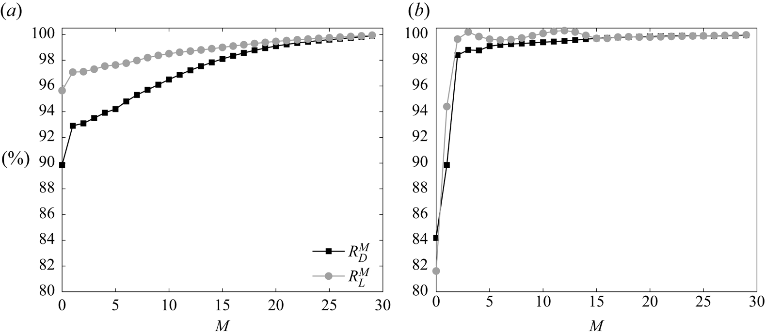
Figure 13. The force convergence indices against the cumulation of mode  $M$ to show the convergence of the force contribution of mode cumulation to drag (black) and lift (grey) for the first thirty modes in cases with (a)
  $AoA = 7.5^\circ$, and (b)
  $AoA = 10^\circ$.
Table 2. Values of the force convergence indices  $\tilde {R}_D^{MN}$ and
  $\tilde {R}_L^{MN}$ in cases with
  $AoA = 7.5^\circ$ and
  $10^\circ$ for
  $0\le M$,
  $N \le 2$.
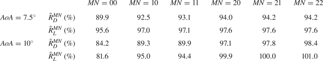
From the previous results, we can conclude that the time variation of the total drag and lift is attributed mainly to the interaction between the zeroth mode and SPOD modes (i.e.  $C^{10}_{D/L,V}$ and
  $C^{20}_{D/L,V}$), whereas the mode–mode interaction (e.g.
  $C^{11}_{D/L,V}$ and
  $C^{22}_{D/L,V}$) provides only fluctuation, which is fairly insignificant to aerodynamic forces. However, it is still difficult to determine the importance of each coherent structure since
  $\bar {\boldsymbol {u}}'^{(m)}$ consists of coherent structures with different time scales/frequencies (Towne et al. Reference Towne, Schmidt and Colonius2018). Therefore, in what follows, we further decompose the flow fields resulting from the first and second SPOD modes (
 $\bar {\boldsymbol {u}}'^{(1)}$ and
  $\bar {\boldsymbol {u}}'^{(2)}$) into the summation of coherent structures oscillating at a single frequency, that is,
 \begin{equation} \bar{\boldsymbol{u}}'^{(m)} = \sum_{k=0}^{{N_{fft}}/{2}} \bar{\boldsymbol{u}}'^{(m,k)},\quad m=1,2, \end{equation}
where  $\bar {\boldsymbol {u}}'^{(m,k)}$ is the velocity of the
  $m$th SPOD mode oscillating at the
  $k$th frequency (i.e. Fourier series expansion of
  $m$th mode). In this study, the evaluation of
  $\bar {\boldsymbol {u}}'^{(m,k)}$ involves nullifying the
  $k$th column vector in (3.18) (
 $k$th frequency in SPOD), followed by the application of (3.19) and (3.20) to convert it to the time domain. Then
  $C^{10}_{D,V}$ and
  $C^{20}_{D,V}$ in (3.24) can be rewritten as
 \begin{equation} \left. \begin{gathered} C^{10}_{D,V} = C^{100}_{D,V}+C^{101}_{D,V}+C^{102}_{D,V}+\cdots+C^{10K}_{D,V},\\ C^{20}_{D,V} = C^{200}_{D,V}+C^{201}_{D,V}+C^{202}_{D,V}+\cdots+C^{20K}_{D,V},\quad \mbox{for }k=N_{fft}/2, \end{gathered} \right\} \end{equation}
where
 \begin{equation} \left. \begin{gathered} C^{10K}_{D,V} = \int_{V_{R}}\left(\bar{\boldsymbol{u}}^{(0)}\times\bar{\boldsymbol{\omega}}'^{(1,K)}+\bar{\boldsymbol{u}}'^{(1,K)}\times\bar{\boldsymbol{\omega}}^{(0)}\right)\boldsymbol{\cdot}\boldsymbol{\nabla}\phi_{1}\,{\rm d}V,\\ C^{20K}_{D,V} = \int_{V_{R}}\left(\bar{\boldsymbol{u}}^{(0)}\times\bar{\boldsymbol{\omega}}'^{(2,K)}+\bar{\boldsymbol{u}}'^{(2,K)}\times\bar{\boldsymbol{\omega}}^{(0)}\right)\boldsymbol{\cdot}\boldsymbol{\nabla}\phi_{1}\,{\rm d}V, \end{gathered} \right\} \end{equation}
are the vorticity force contributions of  $C^{10}_{D,V}$ and
  $C^{20}_{D,V}$ at the
  $K$th frequency. In the following discussions, we refer to
  $K=0$ as the ‘zeroth’ frequency,
  $K=1$ as the ‘first’ frequency, and
  $K=2$ as the ‘second’ frequency. It is worth noting that while
  $C^{10}_{D/L,V}$ (
 $C^{20}_{D/L,V}$) comprises the interaction between the velocity of the zeroth mode and the vorticity of the first (second) mode, as well as the velocity of the first (second) mode and the vorticity of the zeroth mode (see (3.24)), our analysis of the present cases reveals that both components make nearly equal contributions to the drag/lift force. Therefore, our focus lies on the combined effect of these two components.
The procedure of the analysis in the present study is summarized in the flow chart shown in figure 14. We first apply SPOD to the time series of the flow field generated by LES. Subsequently, we reconstruct the flow field for each individual mode and frequency by flow field using the obtained SPOD modes. We then conduct the vorticity force analysis, which enables us to identify force contributions from the mean flow field and coherent structures with various features and frequency. The sum of these contributions is equivalent to the total force obtained from the conventional force analysis.
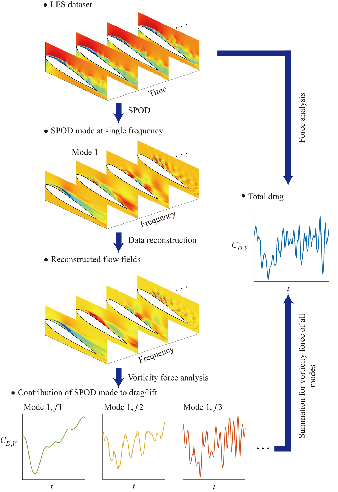
Figure 14. Flow chart summarizing the procedure of the present vorticity force analysis using SPOD. Here, f1, f2 and f3 represent the first, second and third frequencies, respectively.
Figure 15 displays the spectra of the vorticity force contributions to drag and lift for various cases. Specifically, we examine the total force, the zeroth mode, and the cumulation of the first three frequencies of the first mode for cases with  $AoA = 7.5^\circ$ (figures 15a,b) and
  $AoA = 10^\circ$ (figures 15c,d), as well as the second mode for the case with
  $AoA = 10^\circ$ (figures 15e,f). It is important to mention that multiple frequency peaks are observed in figure 15, despite these representing the forces resulting from the SPOD mode at a single frequency. This is due to the fact that we perform SPOD to velocity field rather than
  $C^{10K/20K}_{D/L,V}$. Nonlinear interaction between
  $\bar {\boldsymbol {u}}'^{(m,k)}$ and
  $\bar {\boldsymbol {\omega }}'^{(m,k)}$ in (6.5) will generate frequency peaks different from that generated from SPOD. Another possibility is that the number of sample points (total time step) used in fast Fourier transforms for evaluating spectra of
  $C^{10K/20K}_{D/L,V}$ differs from that utilized in the SPOD procedure (i.e.
  $N_{fft}$ in each block). As a result, multiple frequency peaks are observed in figure 15 due to spectral leakage. Figures 15(a,b) reveal that while there is a gap between the total force and mode cumulation until the second frequency of the first mode (the green line in figures 15a,b), the latter captures a few dominant frequencies corresponding to the large force peak. Although the zeroth and first modes somewhat capture the low-frequency force oscillation, the highest contribution to both drag and lift oscillation cannot be captured until the second mode is added. In contrast to the case with
  $AoA = 7.5^\circ$, where higher frequencies are dominant, the time variations of forces in the case with
  $AoA = 10^\circ$ are dominated by low-frequency oscillations, as shown in figures 15(c–f). These low-frequency oscillations are captured by flow at the zeroth and first frequencies, while flow at the third frequency is responsible for higher-frequency oscillations, which are insignificant in this case. Additionally, the zeroth frequency of the second mode becomes a relatively important contribution to drag, as shown in figure 15(e). Although adding more frequencies in both cases of
  $AoA$ may be desired, for conciseness, the following discussion focuses on the flows at the first three frequencies.

Figure 15. Spectra of the vorticity force contributions to (a,c,e) drag and (b,d,f) lift for the total force, the zeroth mode, and the cumulation of the first three frequencies of the first mode in the cases with (a,b)  $AoA = 7.5^\circ$ and (c,d)
  $AoA = 10^\circ$, and (e,f) the cumulation of the first three frequencies of the second mode in the cases with
  $AoA = 10^\circ$.
7. Vorticity forces of coherent structures in dominant modes and frequencies
7.1.  $AoA = 10^{\circ }$

Figure 16 shows the time histories of the normalized force contribution to drag and lift for the first three frequencies of the first mode in the case with  $AoA = 10^\circ$. It is worthwhile mentioning that in the first mode, the contributions of the zeroth frequency to drag and lift have an opposite trend, and the latter is associated with a greater magnitude. This is explained in the next subsubsection. For the first and second frequencies, patterns of the force contributions to drag and lift are similar. Figure 17 shows results analogous to figure 16 for the second mode. In this mode, the zeroth frequency has a much greater amplitude than the others, and the contribution of the first frequency to drag becomes insignificant. In fact, as shown in figure 9, the first three frequencies in the case with
  $AoA = 10^\circ$ characterize the three important regimes in the velocity spectrum. It should be noted that in the present SPOD, there exists a broadband spectrum at the zeroth frequency, with frequency ranging from
  $St=0$ to
  $St=0.45$. As shown in figure 9, this covers a wide range in the energy containing range of the spectra. This is due to the fact that while SPOD divides the discrete LES data into
  $N_{blk}$ blocks and applies a Fourier transform to each of them (as seen in (3.5) and (3.7)), the highly fluctuated flow pattern does not guarantee that both drag and lift coefficients obtained from the blockwise-averaged flow fields (i.e. zeroth frequency) remain the same in each block. Therefore, there is a low-frequency oscillation (i.e. frequency
  $< N_{blk}/T_{tot}$, where
  $T_{tot}$ is the total simulation time) in the time series of zeroth frequency (see orange line). Variations between blocks will be smoothed after the window-weighted average in frequency domain reconstruction shown in (3.20). Moreover, as documented by Nekkanti & Schmidt (Reference Nekkanti and Schmidt2021), it has been indicated that potentially, the Hamming window (see (3.9)) approach could exhibit abrupt transitions between adjacent blocks, contributing an additional factor of unintended variability in our outcomes. There are two ways to compensate this issue; one is to utilize a greater number of snapshots within a single block, while the other is to extend the duration of the simulation itself. Nevertheless, the effectiveness of both strategies is constrained due to the highly fluctuating characteristics of
  $C_{D/L,V}$ in the current study. Furthermore, utilizing these strategies during the SPOD procedure required massive computational costs. This makes it inefficient to apply them in our study. In summary, the zeroth frequency represents a low-frequency oscillation that results in flapping of the shear layer while the aerofoil is close to stall (Rodriguez et al. Reference Rodriguez, Lehmkuhl, Borrell and Oliva2013). The first and second frequencies (
 $St = 0.86$ and
  $1.7$) are close to the fundamental frequency induced by wakes, while the latter may also indicate a lower bound of the higher-frequency oscillation resulting from shear instability.
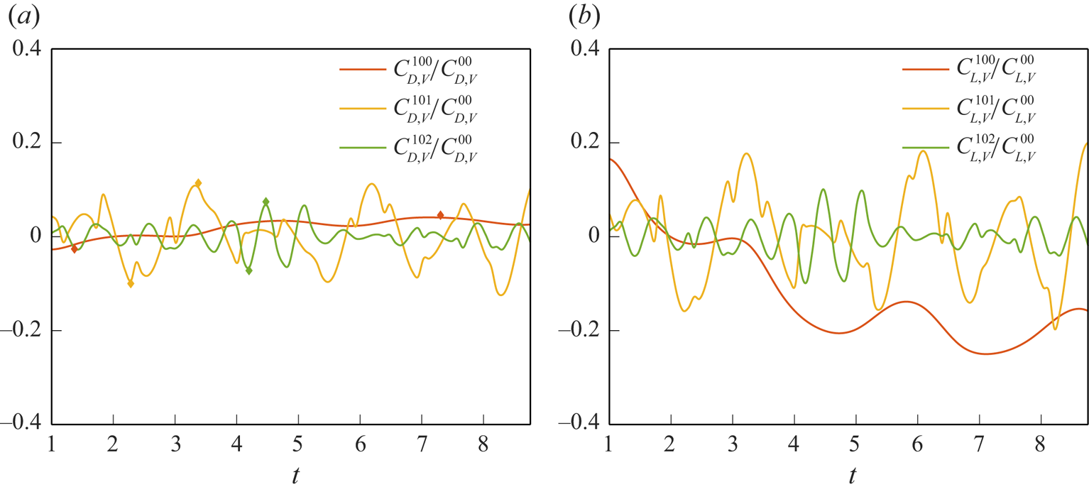
Figure 16. Time histories of the vorticity force contributions to (a) drag and (b) lift, for the first three frequencies of the first mode normalized by the zeroth mode in the case with  $AoA = 10^\circ$. Diamonds in (a) indicate the time points corresponding to local maximum and minimum values of the force contribution.
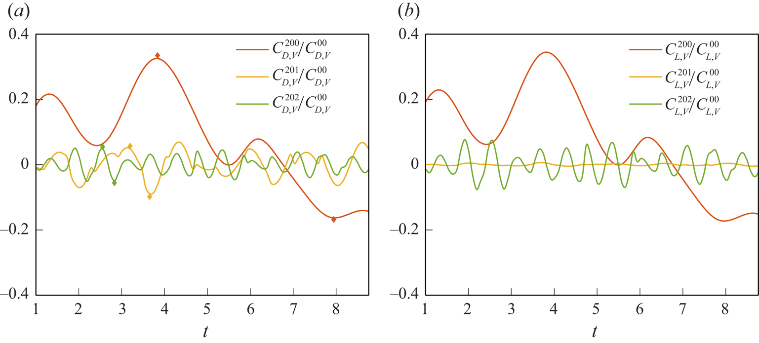
Figure 17. Time histories of the vorticity force contributions to (a) drag and (b) lift, for the first three frequencies of the second mode normalized by the zeroth mode in the case with  $AoA = 10^\circ$. Diamonds in (a) indicate the time points corresponding to local maximum and minimum values of the force contribution.
To examine force contributions of each frequency, we analyse the flow structures resulting from each frequency at the local minimum and maximum, as indicated by diamonds in figures 16(a) and 17(a). Discussion is given in an incremental order in frequency for each mode in a cumulative manner, i.e. discussing the effect of the  $n$th frequency of the
  $m$th mode by adding it to the flow field composed of the zeroth mode and zeroth to
  $(n-1)$th frequencies of the
  $m$th mode. The time points (i.e. local minimum and maximum) taken for the following discussion for a specific mode allows us to minimize the effect of the previous (lower) frequency.
7.1.1. Zeroth frequency of the first mode
Figure 18 presents snapshots of volume drag elements of  $C^{100}_{D,V}$ along with the velocity field at the central slice in the
  $z$-direction and the combination with the zeroth mode at two representative time instants. It should be noted that for better visualization, we use different velocity scales when plotting the flow field for the single frequency (figures 18b,c) and for its combination with its previous mode and frequency (figures 18d,e), as indicated by the arrows at the top right of figures 18(c,e), respectively. All the following figures presenting the analogous physical quantities are plotted in the same manner. As shown in figure 18(a), the positive force contribution at the zeroth mode comes from the strong velocity shear associated with the leading edge separation. It can be seen from figures 18(b,c) that the zeroth frequency of the first mode corresponds to a large vortex structure at the end of the shear layer above the trailing edge. The vortical structure results in a significant stream along the suction side, which interacts with the shear layer, resulting in the low-frequency time variation of drag. At
  $t=1.37$, the vorticity associated with the clockwise rotation is relatively weak, so that the addition of the
  $C^{100}_{D,V}$ to the zeroth mode (see figure 18d) at
  $t=1.37$ does not differ much from the original zeroth mode
  $C^{00}_{D,V}$ shown in figure 18(a). At
  $t=7.30$, the large vortex structure at the same position turns to anticlockwise and becomes stronger, resulting in a significant horizontal stream on the suction side of the aerofoil. As shown in figure 18(e), when combined with the flow of the zeroth mode, the clockwise vortex structure pulls up the shear layer to a higher level and enhances the recirculation near the trailing edge. This results in a leading-edge vortex (LEV) that has a negative force contribution in the region beneath the separated shear layer, which in turn cancels out certain positive contributions in the shear layer. In fact, it is the thin shear layer developed at
  $x = 0.6$–
 $1.8$ on the wall due to the re-entrant jet on the suction side that has a net positive contribution to drag, as shown in figures 18(c,e).
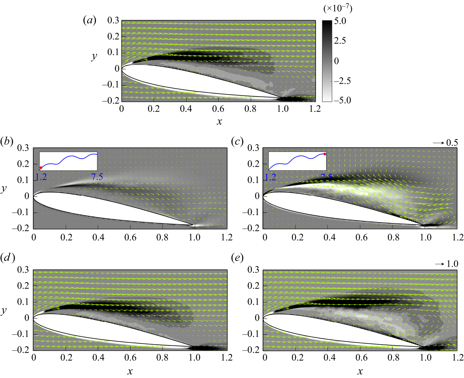
Figure 18. In the case with  $AoA=10^{\circ }$, snapshots of: (a) instantaneous volume drag elements at the central slice in the
  $z$-direction for the zeroth mode superimposed with arrows of
  $\bar {\boldsymbol {u}}^{(0)}$; (b) volume drag elements of
  $C^{100}_{D,V}$ superimposed with arrows of
  $\bar {\boldsymbol {u}}'^{(1,0)}$ at
  $t=1.37$; (c) as (b) but for
  $t=7.30$; (d) volume drag elements of
  $C^{00}_{D,V}+C^{100}_{D,V}$ superimposed with arrows of
  $\bar {\boldsymbol {u}}^{(0)}+\bar {\boldsymbol {u}}'^{(1,0)}$ at
  $t=1.37$; and (e) as (d) but for
  $t=7.30$. The insets in (b,c) indicate the time points on the history of the force contribution of
  $C_{D,V}^{100}$. The arrow at the top right of (c) indicates the velocity scale in (b,c), while the arrow at the top right of (e) indicates the velocity scale in (a,d,e).
In comparison to drag, the volume lift element at the zeroth frequency of the first mode ( $C^{100}_{L,V}$) has a significantly greater magnitude and different sign, as shown in figure 16. To examine this further, figure 19 presents analogous results for
  $C^{100}_{L,V}$. A comparison of the zeroth mode between figures 19(a) and 18(a) shows that the spatial distribution patterns of the volume lift elements are almost identical except near the tip of the leading edge (
 $x < 0.08$), where
  $C_{D,V}^{00}$ turns to the different sign while
  $C^{00}_{L,V}$ remains positive. This different behaviour between drag and lift near the tip of the leading edge is due to the geometric effect, as shown in the auxiliary potential,
  $\phi _1$ and
  $\phi _2$, in figures 2(c,d), respectively. It can be seen from figure 2(c) that when one moves from right to left along the suction side, the positive auxiliary potential for drag (
 $\phi _1$) gradually vanishes and turns negative at the tip of the leading edge, while the auxiliary potential for lift retains a positive sign, as shown in figure 2(d). The non-vanishing of
  $\phi _2$ preserves the positive contribution near the tip of the leading edge at
  $t = 1.37$, as shown in figure 19(b), and the negative contribution at
  $t = 7.30$, as shown in figure 19(c). As a result, contributions to lift have a different sign with greater magnitude when compared to those for drag. This study found that typically, the sign difference feature between contributions to drag and lift is associated with the large vortical structures locating at the shear layer, which induces a significant near-wall stream. This phenomenon is also found in the first frequency of the second mode in the present case with
  $AoA = 10^\circ$, as provided in § 7.1.5.
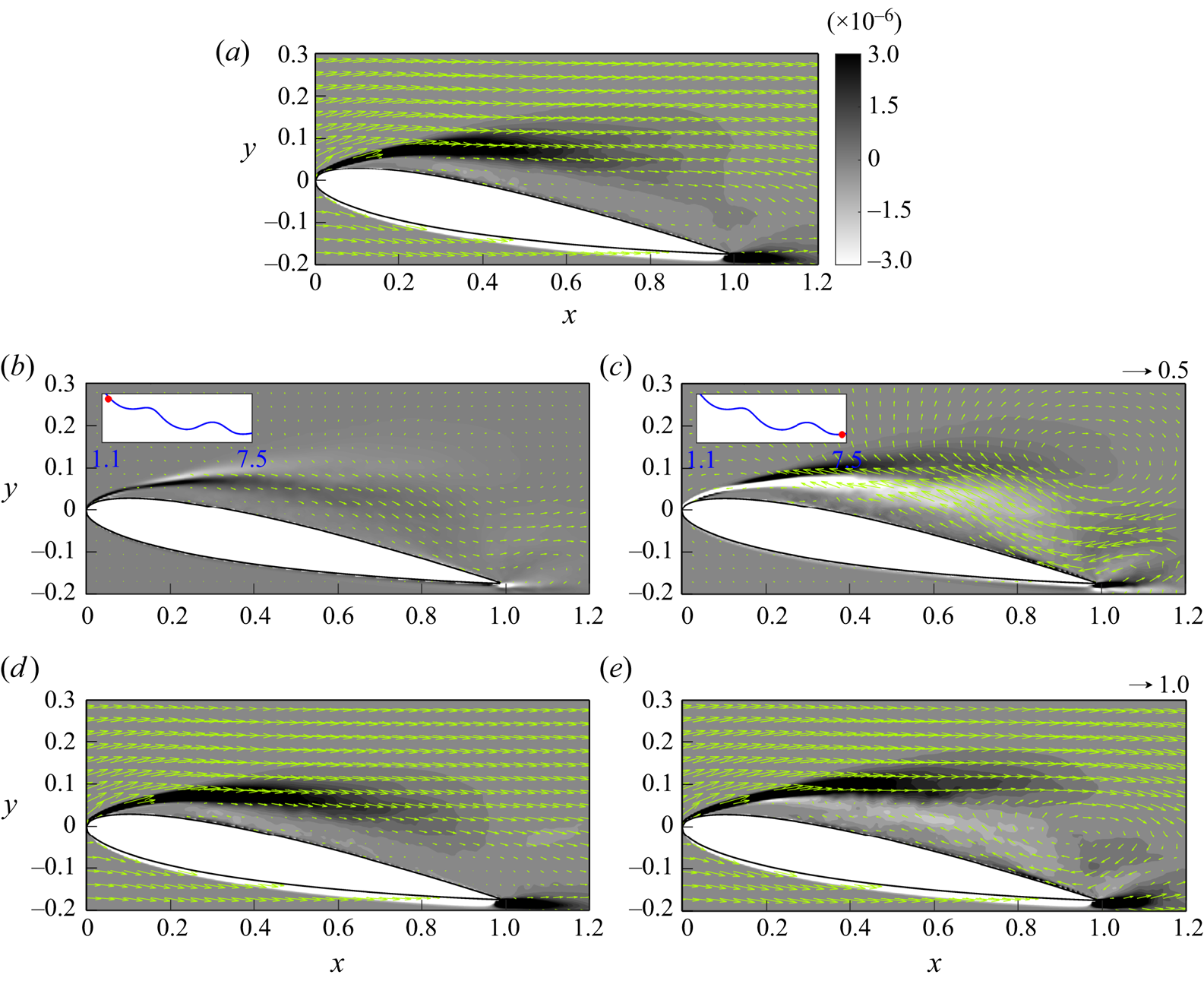
Figure 19. In the case with  $AoA=10^{\circ }$, snapshots of: (a) instantaneous volume lift elements at the central slice in the
  $z$-direction for the zeroth mode superimposed with arrows of
  $\bar {\boldsymbol {u}}^{(0)}$; (b) volume lift elements of
  $C^{100}_{L,V}$ superimposed with arrows of
  $\bar {\boldsymbol {u}}'^{(1,0)}$ at
  $t=1.37$; (c) as (b) but for
  $t=7.30$; (d) volume lift elements of
  $C^{00}_{L,V}+C^{100}_{L,V}$ superimposed with arrows of
  $\bar {\boldsymbol {u}}^{(0)}+\bar {\boldsymbol {u}}'^{(1,0)}$ at
  $t=1.37$; and (e) as (d) but for
  $t=7.30$. The insets in (b,c) indicate the time points on the history of the force contribution of
  $C_{L,V}^{100}$. The arrow at the top right of (c) indicates the velocity scale in (b,c), while the arrow at the top right of (e) indicates the velocity scale in (a,d,e).
7.1.2. First frequency of the first mode
Figure 20 shows snapshots of volume drag elements of  $C^{101}_{D,V}$ at the central slice in the
  $z$-direction and its combination with
  $C^{00}_{D,V}$ and
  $C^{100}_{D,V}$ at two representative time instants. The first frequency corresponds to an asymmetric vortex pair, with one vortex located ahead of and the other behind the trailing edge. As shown in figures 20(a,b), the strong flow pointing to the top left at
  $t=2.28$ leads to the negative contribution to drag, while the flow pointing to the bottom right at
  $t=3.38$ provides a positive contribution to drag. When combined with the previous mode and frequency, at
  $t=2.28$, the anticlockwise vortex suppresses the shear layer in the zeroth mode (see figure 20c). When the vortex turns clockwise, similar to that in
  $C^{100}_{D,V}$ (see figure 18e), an LEV is formed ahead of the trailing edge, which slightly enhances the positive contribution to drag, as shown in figure 20(d). Both the zeroth and first frequencies of the first mode correspond to the LEV, but the latter is more localized, such that its major influence is limited into the second half of the chord (
 $x = 0.6$–
 $1.0$).

Figure 20. In the case with  $AoA=10^{\circ }$, snapshots of: the instantaneous volume drag elements at the central slice in the
  $z$-direction for volume drag elements of
  $C^{101}_{D,V}$ superimposed with arrows of
  $\bar {\boldsymbol {u}}'^{(1,1)}$ at (a)
  $t=2.28$, and (b)
  $t=3.38$; and volume drag elements of
  $C^{00}_{D,V}+\sum _{K=0}^{1} C^{10K}_{D,V}$ superimposed with arrows of
 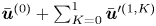 $\bar {\boldsymbol {u}}^{(0)}+ \sum _{K=0}^{1}\bar {\boldsymbol {u}}'^{(1,K)}$ at (c)
  $t=2.28$, and (d)
  $t=3.38$. The insets in (a,b) indicate the time points on the history of the force contribution of
  $C_{D,V}^{101}$. The arrow at the top right of (b) indicates the velocity scale in (a,b), while the arrow at the top right of (d) indicates the velocity scale in (c,d).
7.1.3. Second frequency of the first mode
Figure 21 presents snapshots of volume drag elements of  $C^{102}_{D,V}$ superimposed with the corresponding velocity field at the central slice in the
  $z$-direction, at two representative time instants. The flow field of the second frequency of the first mode consists of a series of vortex pairs at the separated shear layer, namely shear-layer vortices (SLV). These high-frequency, low-wavelength wakes arise due to instability at the separated shear layer. As we can use vorticity force analysis to evaluate forces generated by vortices, it is worth noting that a single vortex has zero net force contribution without background flow; it is the combination of a vortex and background stream that generates a net vorticity force. Therefore, the upper half-regions of these vortices, located in the shear layer, are associated with a stronger drag contribution. Figure 21 also shows that the clockwise vortical structure, which supports the shear layer, provides a positive drag contribution, while the anticlockwise vortical structure, which somewhat disrupts the shear layer, has a negative drag contribution.

Figure 21. Snapshots of the instantaneous volume drag elements at the central slice in the  $z$-direction for
  $C^{102}_{D,V}$ superimposed with arrows of
  $\bar {\boldsymbol {u}}'^{(1,2)}$ at (a)
  $t=4.20$, and (b)
  $t=4.47$, in the case with
  $AoA=10^{\circ }$. The insets indicate the time points on the history of the force contribution of
  $C_{D,V}^{102}$. The arrow at the top right of (b) indicates the velocity scale in (a,b).
To examine further the contribution of these high-frequency wakes, figure 22 presents snapshots of volume drag elements due to the combination of the first three frequencies of the first mode and the zeroth mode at the central slice in the  $z$-direction superimposed with the associated velocity field. The figure also presents the corresponding iso-surfaces of the
  $Q$-criterion (Hunt, Wray & Moin Reference Hunt, Wray and Moin1988) of the original flow field (
 $Q=5\times 10^5$) superimposed with volume drag elements of
  $C_{D,V}$ at four representative time instants. It can be seen that the clockwise vortical structure at the middle of the chord (
 $x \sim 0.6$) in figure 21 corresponds to an enlarged area of positive contribution in the shear layer in figure 22(a). In the original flow field, as shown in figure 22(b), it represents an expanding spanwise vortex originating from the leading-edge separation due to shear instability, as indicated by the triangle in figure 22(b). The downstream movement of this vortical structure along the separated shear layer farther from the wall (see figure 22c) represents a roll-up of the spanwise vortex, accompanied by three-dimensional vortical structures (e.g. distortion and streamwise vortices), as shown in figure 22(d). At this moment, the flow at the second frequency of the first mode approaches a local maximum of the force contribution to drag, as shown in the inset of figure 22(c). The distortion of the two-dimensional vortex core leads to a horseshoe-like vortical structure, as shown in figures 22(d,f). The further roll-up of the vortical structure towards the downstream, as shown in figures 22(e,g), leads to the irregularity of the vortical structure, followed by the break-up and movement away from the aerofoil's surface, as shown in figure 22(h), which reduces its drag contribution (see figure 22g).
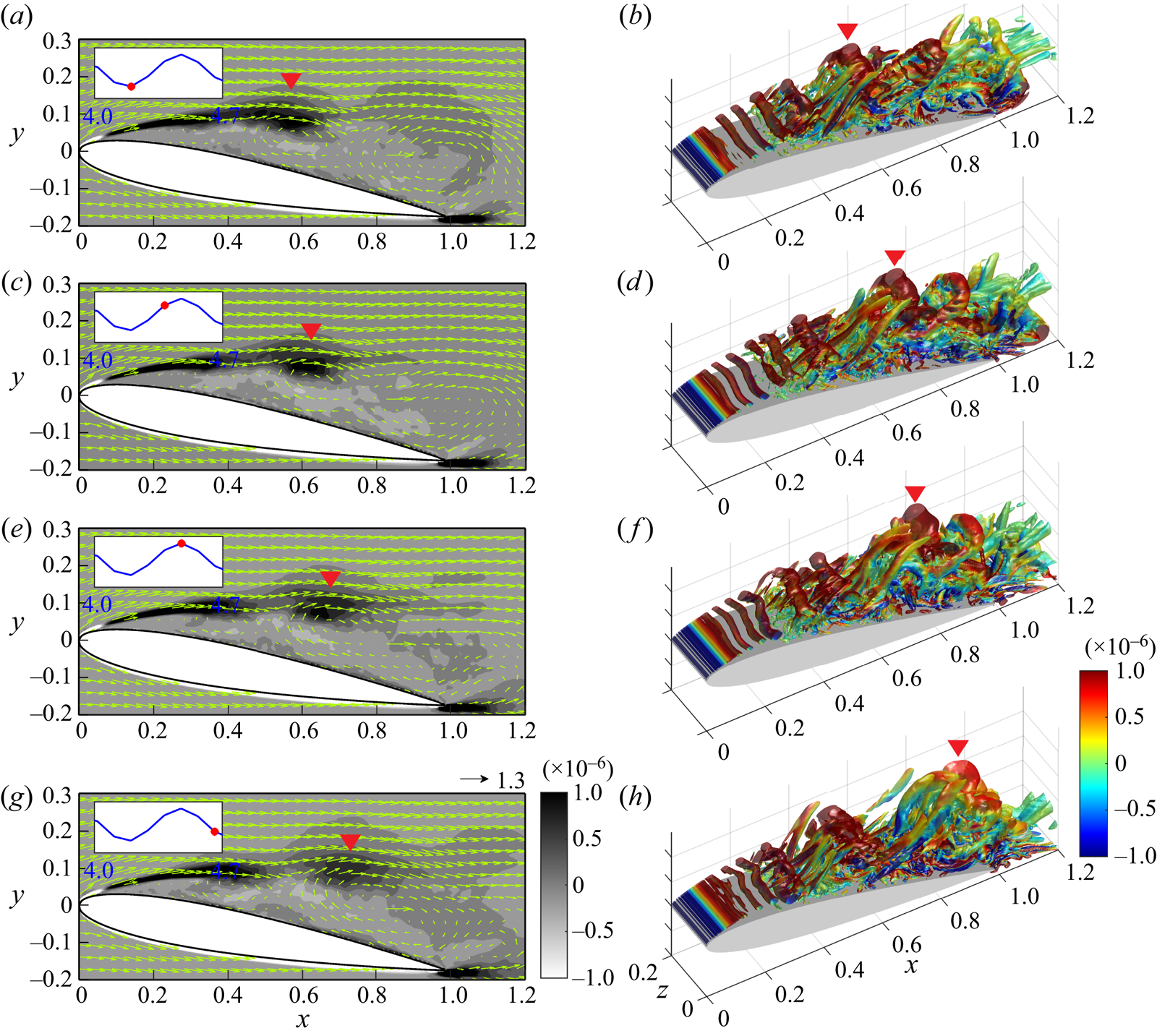
Figure 22. Snapshots of (a,c,e,g) the instantaneous volume drag elements due to the zeroth mode and the first three frequencies of the first mode at the central slice in the  $z$-direction superimposed with the associated velocity field, and (b,d,f,h) the corresponding iso-surfaces of the
  $Q$-criterion (
 $Q = 5\times 10^5$), coloured with volume drag elements at (a,b)
  $t = 4.20$, (c,d)
  $t = 4.38$, (e,f)
  $t = 4.47$, and (g,h)
  $t = 4.67$, in the case with
  $AoA = 10^\circ$. The insets in (a,c,e,g) indicate the corresponding points on the time history of the force contribution of the second frequency of the first mode. The arrow at the top right of (g) indicates the velocity scale in (a,c,e,g). The red triangles indicate the downstream evolution of a vortical structure in (a,c,e,g) the reduced flow field, and (b,d,f,h) the original flow field.
7.1.4. Zeroth frequency of the second mode
Here, we conduct the same analyses as in §§ 7.1.1–7.1.3, and focus on the contributions of the first three frequencies of the second mode. Figure 23 shows snapshots of volume drag elements of  $C^{200}_{D,V}$ at the central slice in the
  $z$-direction and its combination with the zeroth mode at two representative time instants (see figure 17a). Similar to volume drag elements of
  $C^{100}_{D,V}$ (see figure 18), we observe a clockwise primary LEV near the trailing edge of the aerofoil, and a strong, thin layer on the surface of the aerofoil is observed at
  $t=3.83$, resulting in a maximum value of drag (see figure 23a). In contrast, at
  $t=7.85$, the anticlockwise LEV provides a negative contribution to drag on the surface of the aerofoil, as shown in figure 23(b). Furthermore, when adding volume drag elements of
  $C^{200}_{D,V}$ to the zeroth mode, we observe that the clockwise LEV causes a downstream extension of the shear layer and creates a circulation zone near the trailing edge, as shown in figure 23(c). On the other hand, the anticlockwise LEV destroys the shear layer of the zeroth mode, as shown in figure 23(d).
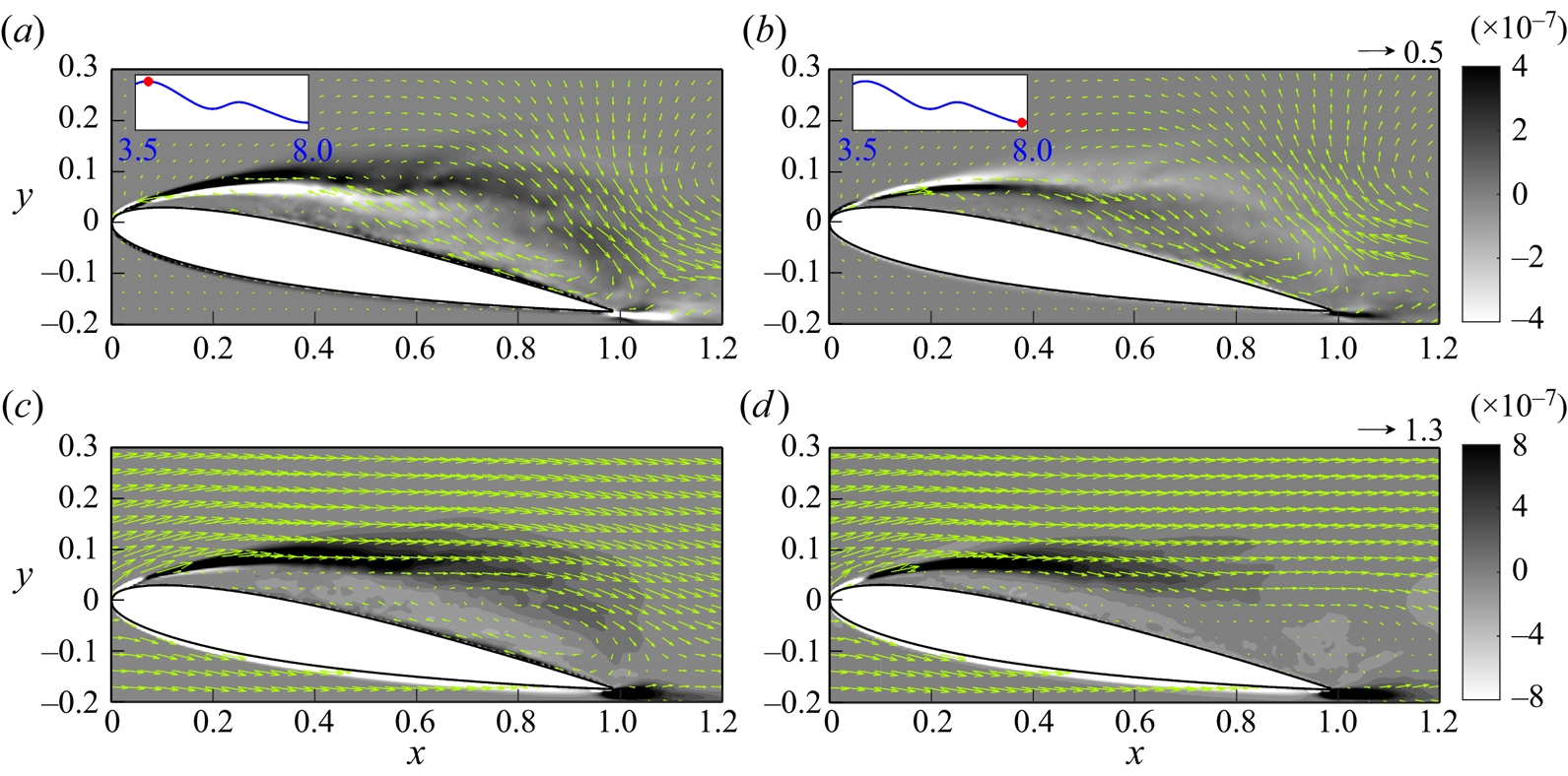
Figure 23. In the case with  $AoA=10^{\circ }$, snapshots of: the instantaneous volume drag elements at the central slice in the
  $z$-direction for volume drag elements of
  $C^{200}_{D,V}$ superimposed with arrows of
  $\bar {\boldsymbol {u}}'^{(2,0)}$ at (a)
  $t=3.83$, and (b)
  $t=7.85$; and volume drag elements of
 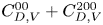 $C^{00}_{D,V}+C^{200}_{D,V}$ superimposed with arrows of
  $\bar {\boldsymbol {u}}^{(0)}+\bar {\boldsymbol {u}}'^{(2,0)}$ at (c)
  $t=3.83$, and (d)
  $t=7.85$. The insets in (a,b) indicate the time points on the history of the force contribution of
  $C_{D,V}^{200}$. The arrow at the top right of (b) indicates the velocity scale in (a,b), while the arrow at the top right of (d) indicates the velocity scale in (c,d).
7.1.5. First frequency of the second mode
Figure 24 shows snapshots of volume drag elements of  $C^{201}_{D,V}$ at the central slice in the
  $z$-direction, superimposed with the flow field at two representative time instants, for combination with the volume drag elements of
  $C^{00}_{D,V}$ and
  $C^{200}_{D,V}$. From figures 24(a,b), it can be observed that the flow at the first frequency of the second mode corresponds to a vortex located at the shear layer at
  $x = 0.6$–
 $0.8$, and a vortex near the tip of the trailing edge, known as the trailing-edge vortex (TEV). The former is similar to those found in the zeroth frequency of the first mode, but has a smaller size and is closer to the middle of the chord. As shown in figure 21, drag is enhanced due to clockwise rotation and suppressed due to anticlockwise rotation. In this case, the TEV does not contribute significantly to drag when combined with the zeroth mode and zeroth frequency. However, its contribution to drag is explained when examining the second frequency in § 7.1.6. It is worth noting that in figure 17, contributions to drag and lift have different signs, whereas the latter is associated with a significantly smaller magnitude. This is similar to the zeroth frequency of the first mode, which is due to the geometric effect near the tip of the leading edge (see § 7.1.1).
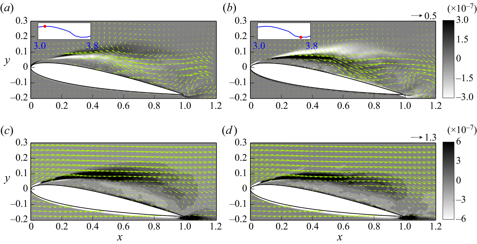
Figure 24. Snapshots of the instantaneous volume drag elements at the central slice in the  $z$-direction superimposed with the associated flow field for the first frequency of the second mode at (a)
  $t = 3.10$ and (b)
  $t = 3.65$, and the cumulation of the first frequency of the first mode combined with the zeroth mode at (c)
  $t = 3.10$ and (d)
  $t = 3.65$, in the case with
  $AoA = 7.5^\circ$. The insets in (a,b) indicate the time points on the history of the force contribution of
  $C_{D,V}^{201}$. The arrow at the top right of (b) indicates the velocity scale in (a,b), while the arrow at the top right of (d) indicates the velocity scale in (c,d).
7.1.6. Second frequency of the second mode
Figure 25 shows snapshots of volume drag elements of  $C^{202}_{D,V}$ at the central slice in the
  $z$-direction, in combination with the volume drag elements of
  $C^{00}_{D,V}$,
  $C^{200}_{D,V}$ and
  $C^{201}_{D,V}$, with the flow field at two representative time instants superimposed. Although there are insignificant vortical structures along the shear layer similar to the second frequency of the first mode (see § 7.1.3), the most notable flow feature is the presence of the TEV, as shown in figures 25(a,b). When combined with the flow field of the zeroth mode and the previous two frequencies, as shown in figures 25(c,d), the structure of the TEV becomes less apparent. However, it can be observed that the TEV with anticlockwise rotation (see figure 25a) slightly enhances drag at the tip of the trailing edge (figure 25c), while its clockwise rotation (figure 25b) suppresses drag (figure 25d).

Figure 25. Snapshots of the instantaneous volume vorticity drag elements at the central slice in the  $z$-direction for
  $C^{202}_{D,V}$ superimposed with arrows of
  $\bar {\boldsymbol {u}}'^{(2,2)}$ at (a)
  $t=5.39$, and (b)
  $t=5.84$, and volume drag elements of
  $C^{00}_{D,V}+\sum _{K=0}^{2} C^{20K}_{D,V}$ superimposed with arrows of
  $\bar {\boldsymbol {u}}^{(0)}+ \sum _{K=0}^{2}\bar {\boldsymbol {u}}'^{(2,K)}$ at (c)
  $t=5.39$, and (d)
  $t=5.84$, in the case with
  $AoA=10^{\circ }$. The arrow at the top right of (b) indicates the velocity scale in (a,b), while the arrow at the top right of (d) indicates the velocity scale in (c,d).
7.2. $AoA = 7.5^\circ$

Figure 26 displays the time histories of the normalized force contribution to drag and lift for the first three frequencies of the first mode in the case with  $AoA = 7.5^\circ$. Owing to flow reattachment, fluctuations in force contributions to both drag and lift are lower compared to the larger
  $AoA$ cases depicted in figures 16 and 17. Despite the negligible contribution of the zeroth mode to lift, the fluctuation patterns are fairly similar between drag and lift. To examine the force contribution of each dominant frequency, we analyse the resulting flow structures resulting from each frequency at the local minimum and maximum, as indicated by the diamonds in figure 26(a).
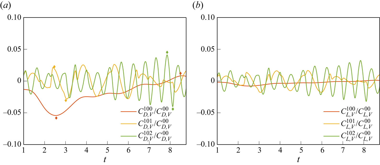
Figure 26. Time histories of the vorticity force contributions to (a) drag and (b) lift, for the first three frequencies of the first mode normalized by the zeroth mode in the case with  $AoA = 7.5^\circ$. Diamonds in (a) indicate the time points corresponding to local maximum and minimum values of the force contribution, which are used for further analysis in § 7.2.
7.2.1. Zeroth frequency of the first mode
Figure 27 presents snapshots of volume drag elements of  $C^{00}_{D,V}$ and
  $C^{100}_{D,V}$ (i.e. the zeroth frequency of the first mode) at the central slice in the
  $z$-direction for combination with the volume drag elements of
  $C^{00}_{D,V}$ superimposed with the flow field at two representative time instants in the case with
  $AoA = 7.5^\circ$. As shown in figure 27(a), the shear layer associated with the leading-edge separation dominates the drag contribution. The drag contribution vanishes near the reattachment point at
  $x \sim 0.5$, indicating that the flow reattachment suppresses drag. As shown in figures 27(b,c), the zeroth frequency of the first mode corresponds to an oscillating near-wall stream that follows the pattern of the reattachment flow. The positive stream of the zeroth frequency slightly hinders the downstream development of the separated shear layer such that the drag decreases, as shown in figure 27(b). In contrast, as shown in figure 27(c), the near-wall backflow at the zeroth frequency enhances the development of the shear layer, thus increasing its drag contribution. That is, when
  $AoA = 7.5^\circ$, the zeroth frequency of the first mode corresponds to a periodic motion of back-and-forth movement of the reattachment point, for which the early reattachment can result in a decrease in drag, and vice versa.
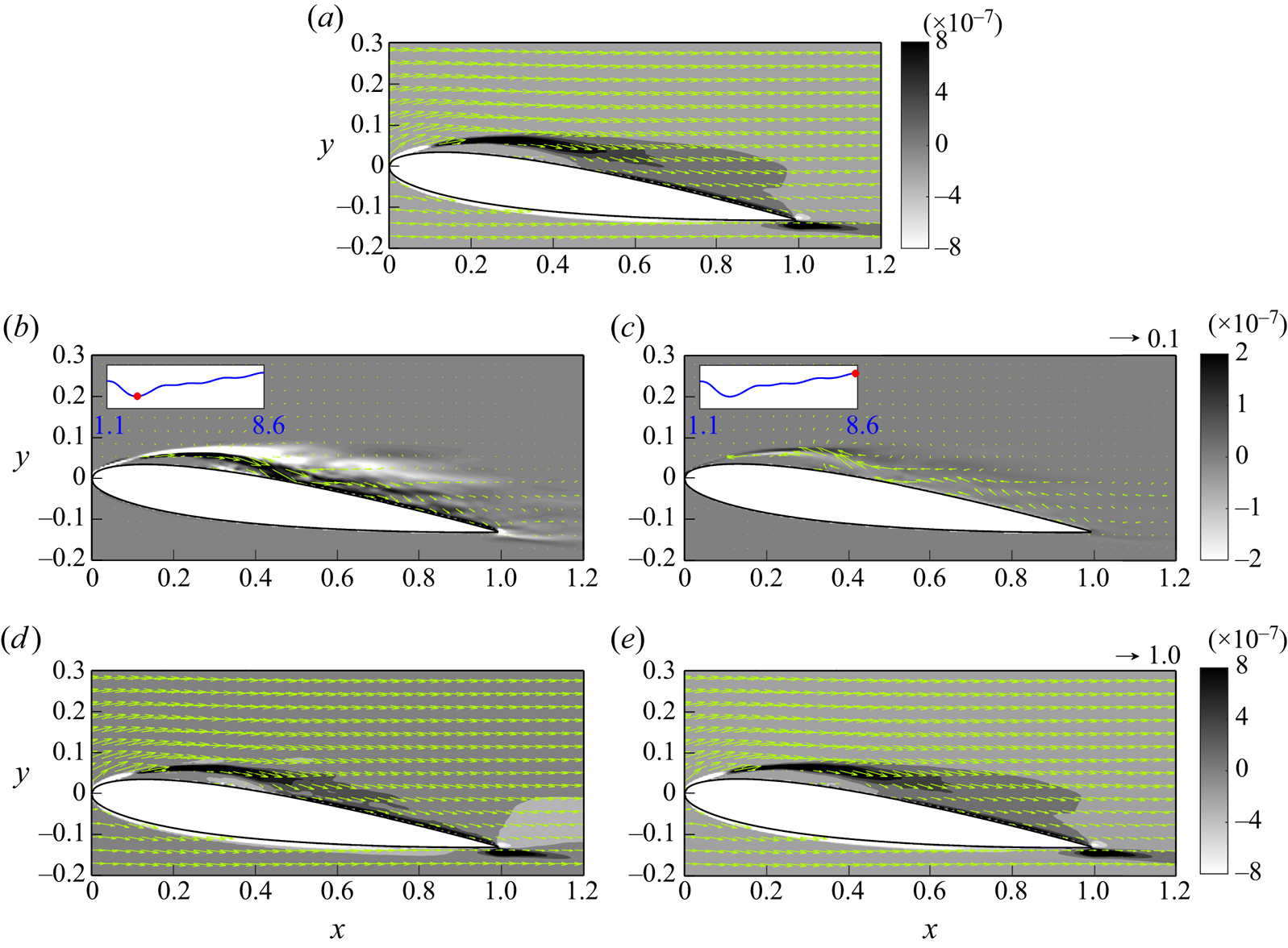
Figure 27. Snapshots of the instantaneous volume drag elements at the central slice in the  $z$-direction superimposed with the associated flow field for (a) the zeroth mode, (b) the zeroth frequency of the first mode at
  $t = 2.56$, and (c) the same as (b) but for
  $t = 8.49$, and its combination with the zeroth mode at (d)
  $t = 2.56$, and (e)
  $8.49$, in the case with
  $AoA = 7.5^\circ$. The insets in (b,c) indicate the time points on the history of the force contribution of
  $C_{D,V}^{200}$. The arrow at the top right of (c) indicates the velocity scale in (b,c), while the arrow at the top right of (e) indicates the velocity scale in (a,d,e).
7.2.2. First frequency of the first mode
Figure 28 displays snapshots of volume drag elements of  $C^{101}_{D,V}$ along with the velocity field at the central slice in the
  $z$-direction for combination with the zeroth mode and the first frequency at two representative time instants in the case with
  $AoA = 7.5^\circ$. As shown in figures 28(a,b), the first frequency corresponds to a counter-rotating vortex pair that generates the near-wall stream. The vortex pair originates at the point where the flow reattaches (
 $x \approx 0.5$). Due to the weakened shear caused by flow reattachment, the influence of the vorticity on drag is reduced significantly. In fact, the drag contribution of these large-scale vortex structures is similar to that in the zeroth mode, which corresponds to the back-and-forth motion of the reattachment resulting from the near-wall stream, as shown in figures 28(c,d).
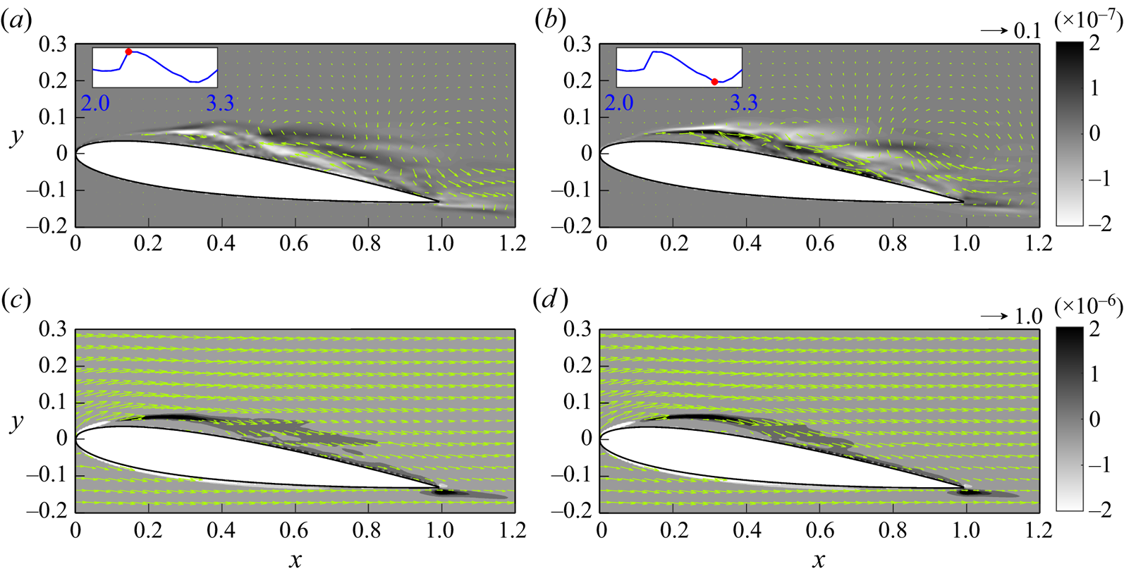
Figure 28. Snapshots of the instantaneous volume drag elements at the central slice in the  $z$-direction superimposed with the associated flow field for the first frequency of the first mode at (a)
  $t = 2.47$ and (b)
  $t = 2.92$, and the cumulation of the first frequency of the first mode combined with the zeroth mode at (c)
  $t = 2.56$, and (d)
  $t = 2.47$, in the case with
  $AoA = 7.5^\circ$. The insets in (a,b) indicate the time points on the history of the force contribution of
  $C_{D,V}^{201}$. The arrow at the top right of (b) indicates the velocity scale in (a,b), while the arrow at the top right of (d) indicates the velocity scale in (c,d).
7.2.3. Second frequency of the first mode
Figure 29 shows snapshots of volume drag elements of  $C^{102}_{D,V}$, along with the velocity field at the central slice in the
  $z$-direction for the combination of the zeroth mode and the previous frequencies at two representative time instants in the case with
  $AoA = 7.5^\circ$. Similar to
  $AoA = 10^\circ$, the second frequency of the first mode in this case corresponds to a series of smaller counter-rotating vortex pairs at the shear layer originated near the point of flow reattachment, as shown in figures 29(a,b). The clockwise vortex provides a positive drag contribution, while the anticlockwise vortex provides a negative contribution. It is found that only those vortices located near the reattachment point provide relatively significant effect on drag, as shown in figures 29(c,d), due to flow reattachment.
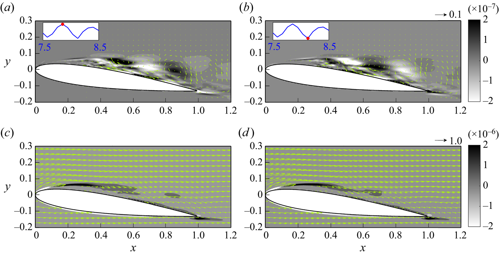
Figure 29. Snapshots of the instantaneous volume drag elements at the central slice in the  $z$-direction superimposed with the associated flow field for the second frequency of the first mode at (a)
  $t = 7.85$, and (b)
  $t = 8.13$, and the cumulation of the second frequency of the first mode combined with the zeroth mode at (c)
  $t = 7.85$ and (d)
  $t = 8.13$, in the case with
  $AoA = 7.5^\circ$. The insets in (a,b) indicate the time points on the history of the force contribution of
  $C_{D,V}^{202}$. The arrow at the top right of (b) indicates the velocity scale in (a,b), while the arrow at the top right of (d) indicates the velocity scale in (c,d).
It can be observed that in the case with  $AoA = 7.5^\circ$, the separated shear layer resulting from flow reattachment vanishes, and vorticity forces in the non-zero mode are effective only near the reattachment point, rapidly becoming negligible as one moves further downstream from the reattachment point. This limits the major source of drag and lift only at the reattachment point, resulting in the force fluctuations being significantly suppressed compared to the large
  $AoA$ case.
7.3. Quantitative comparison of SPOD modes and force contribution
Figure 30 displays representative snapshots of the iso-surfaces of the reconstructed vertical velocity of the first three frequencies (including the zeroth frequency) of the first mode (i.e.  $v'^{(1,m)}$) for
  $AoA = 7.5^\circ$, and first and second modes for
  $AoA = 10^\circ$ (i.e.
  $v'^{(1,m)}$ and
  $v'^{(2,m)}$), at
  $t=4.29$ where the local maximum of drag is observed (see figure 10). As is typical in mode decomposition, the wavelength of flow fluctuations decreases with increasing frequency. The wavelengths, which are obtained by applying the fast Fourier transform to the flow field, along with the type description for each frequency and mode, are summarized in table 3. Generally, the zeroth and first frequencies correspond to changes of LEV, while the second frequency corresponds to SLV. In the case of larger
  $AoA$, a TEV can be found in the first and second frequencies of the second mode. A quantitative measure of these representative frequencies and modes is conducted by examining their r.m.s. values shown in figures 16, 17 and 26 with respect to the zeroth mode. The obtained values are also summarized in table 3. One interesting point is that although the first SPOD mode captures most of the turbulent kinetic energy (see figure 12), the resulting vorticity forces do not follow the same trend. That is, the highest energy mode does not necessarily correspond to the greatest vorticity force fluctuation. As shown in table 3, the r.m.s. of
  $C^{200}_{D,V}$ (
 $15.6\,\%$) is much larger than that of each frequency in the first SPOD mode. However, due to the geometry effect discussed in § 7.1.1, the r.m.s. of
  $C^{100}_{L,V}$ is slightly larger than that of
  $C^{200}_{L,V}$. According to the present theory, in addition to the flow strength, the contribution of each SPOD mode also depends on the location relative to the aerofoil.
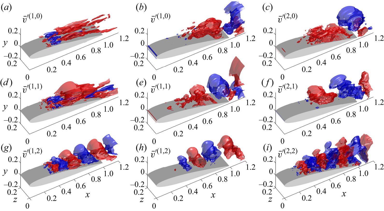
Figure 30. Snapshots of the iso-surfaces of the vertical velocity component for the zeroth to second frequencies (from top to bottom) of (a,d,g) the first mode in the case with  $AoA = 7.5^\circ$, and (b,e,h) the first and (c,f,i) the second modes in the case with
  $AoA = 10^\circ$, at
  $t = 4.29$ where the local maximum of drag occurs. The red and blue iso-surfaces represent positive and negative values, which are (a) 0.01 and
  $-$0.03, (b) 0.1 and
  $-$0.05, (c) 0.04 and
  $-$0.1, (d) 0.01 and
  $-$0.03, (e) 0.003 and
  $-$0.015, (f) 0.05 and
  $-$0.03, (g) 0.01 and
  $-$0.01, (h) 0.15 and
  $-$0.15, and (i) 0.02 and
  $-$0.02.
Table 3. Wavelengths, normalized r.m.s. vorticity force contributions, and flow features in representative frequencies and modes in the cases with  $AoA = 7.5^\circ$ and
  $10^\circ$. In the fifth and sixth columns, the superscript
  $m$ represents the mode number, and
  $n$ is the frequency number.
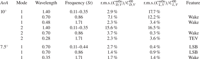
In the case of small  $AoA$, differences in the force contribution between different frequencies are not significant, and it is difficult to ascertain the relative importance of each mode from table 3. When
  $AoA$ becomes larger, the dominant role of the zeroth frequency in vorticity forcing can be found in the first mode in lift, and the second mode in both lift and drag. Moreover, forces are typically dominated by a TEV (i.e. a combination of the zeroth and first frequencies), while SLV and TEVs are responsible for high-frequency fluctuations with lower strength. The reduction in the force contribution of the zeroth frequency in the case with
  $AoA = 7.5^\circ$ compared with
  $AoA = 10^\circ$ demonstrates a significant suppression of force fluctuations due to flow reattachment.
8. Concluding remarks
In the present study, a series of analyses focused on the aerodynamic forces exerted by coherent structures on the NACA0012 aerofoil. These analyses were conducted at two different angles of attack, specifically  $AoA=7.5^{\circ }$ and
  $10^{\circ }$, with a chord-based Reynolds number
  $Re=50\,000$. To identify the coherent structures in turbulent flows, the SPOD algorithm was employed. This involved analysing a considerable amount of LES data, and the resulting SPOD modes in the frequency domain were transformed back into the time domain. The vorticity force analysis (Chang Reference Chang1992) was utilized to quantify the impact of coherent structures on drag and lift forces. This allowed us to calculate the drag and lift coefficients by adding up the effects of the interactions between the zeroth mode flow field and the SPOD modes, as well as the interactions between different modes. It has been noted that the former is responsible for the overall variation of the drag and lift forces, whereas the latter contributes only to the small fluctuations in the time variation.
At an angle of attack  $AoA=10^{\circ }$, we examined the distribution of volume vorticity force (i.e.
  $C_{D,V}$) for the zeroth, first and second frequencies of the first two SPOD modes. The zeroth frequency of the first SPOD mode corresponds to a large vortex structure at the end of the shear layer above the trailing edge. This structure causes a strong flow along the suction side of the aerofoil, resulting in a significant impact on the drag and lift forces based on the rotation directions of the vortex. Additionally, the combination with the zeroth mode confirms that the shear layer is pulled up by the clockwise vortex, and a leading-edge vortex (LEV) is formed. Due to the geometry effect of
  $\phi _{2}$, contributions to lift have different sign with greater magnitude when compared to those for drag, even though both share the same coherent structure. The first frequency of the first SPOD mode represents an asymmetric vortex pair. The interaction between this vortex pair generates a top left stream that destroys the shear layer and causes a negative contribution to drag, while the bottom right stream creates a localized LEV and provides a positive contribution. As for the second frequency of the first SPOD mode, we found a series of vortex pairs present at the shear layer (SLV). Following the downstream movement of SLV, we concluded that the leading-edge separation results in the drag enhancement since the clockwise vortical structure provides a positive drag contribution. Moreover, these vortical structures represent a roll-up of the spanwise vortex, which leads to an irregularity of the vortical structure followed by its break-up and movement away from the aerofoil's surface.
The same analyses are conducted for the zeroth frequency of the second SPOD modes. A clockwise primary LEV near the trailing edge of the aerofoil provides a positive contribution to drag, while an anticlockwise LEV provides a negative contribution. When the second SPOD mode is added to the zeroth mode, the clockwise LEV causes a downstream extension of the shear layer and creates a circulation zone near the trailing edge, while the anticlockwise LEV destroys the shear layer of the zeroth mode. The flow at the first frequency of the second SPOD mode consists of a vortex located at the shear layer and a vortex near the trailing-edge tip. The drag is enhanced due to clockwise rotation and suppressed due to anticlockwise rotation. The significant flow feature of the second frequency of the second SPOD mode is the trailing-edge vortex (TEV), which enhances drag with anticlockwise rotation and suppresses drag with clockwise rotation. When combined with other modes, the structure of the TEV becomes less apparent. There are insignificant vortical structures along the shear layer similar to the second frequency of the first mode.
In the case with  $AoA=7.5^{\circ }$, the zeroth frequency of the first mode corresponds to an oscillating near-wall stream that follows the reattachment flow pattern. The positive stream slightly hinders the separated shear layer development, decreasing drag, while the near-wall backflow enhances the development of the shear layer, increasing the drag contribution. The first frequency corresponds to a counter-rotating vortex pair originating where the flow reattaches. The weakened shear due to flow reattachment reduces the drag contribution of these large-scale vortex structures, making them similar to the back-and-forth motion of the reattachment resulting from the near-wall stream in the zeroth mode. Finally, the second frequency of the first mode corresponds to smaller counter-rotating vortex pairs at the shear layer originated near the reattachment point. The vorticity forces in the non-zero mode are effective only near the reattachment point, and flow reattachment in the smaller
  $AoA$ case significantly suppresses force fluctuations compared to the large
  $AoA$ case.
Funding
We gratefully acknowledge the support of the Taiwan Ministry of Science and Technology (MOST) Thermal Science and Fluid Dynamic Program under grant no. MOST 109-2221-E-002-028-MY3.
Declaration of interests
The authors report no conflict of interest.
Appendix A. Convergence of SPOD modes
Following Sano et al. (Reference Sano, Abreu, Cavalieri and Wolf2019) and Abreu et al. (Reference Abreu, Tanarro, Cavalieri, Schlatter, Vinuesa, Hanifi and Henningson2021), in order to assess the convergence of the SPOD modes generated with the current set-up, we partitioned the original dataset into two blocks. Each block consisted of  $75\,\%$ of the original dataset, equivalent to
  $750$ snapshots. The procedures outlined in § 3.1 were then applied independently to each block, resulting in corresponding SPOD modes denoted by
  $\phi _{i,M}$. Here, the subscript
  $i$ indicates the index of the sub-dataset, while
  $M$ denotes the mode index. A convergence index
  $\beta _{i,M}$ is defined by normalizing the inner product between
  $\phi _{M}$ (original SPOD mode) and
  $\phi _{i,M}$:
 \begin{equation} \beta_{i,M} = \dfrac{\langle\phi_{M},\phi_{i,M}\rangle}{\sqrt{\left\vert\left\vert\phi_{M}\right\vert\right\vert\times\vert\vert\phi_{i,M}\vert\vert}}, \end{equation}
where  $\langle \,\cdot\, \rangle$ is the inner product, and
  $\vert \vert \cdot \vert \vert$ represents the
  $L_{2}$ norm of the vector. Equation (A1) quantifies the degree of similarity between the original dataset's mode
  $\phi _{M}$ and the mode obtained from the sub-dataset,
  $\phi _{i,M}$. A value of
  $\beta _{i,M}$ close to
  $1$ indicates that
  $\phi _{i,M}$ and
  $\phi _{M}$ are highly similar, hence the current set-up achieves mode convergence.
The convergence index  $\beta _{i,M}$ for the zeroth, first, and second frequencies is shown in figure 31 for the cases with
  $AoA=7.5^{\circ }$ and
  $AoA=10^{\circ }$. It is evident that
  $\beta _{i,M}$ is highly dependent on the number of snapshots used in the analysis, especially for higher modes, as it is sensitive to the limited number of snapshots (i.e.
  $1000$) used in this study. Despite this, the first two modes of each frequency were found to be well converged with
  $\beta _{i,M}\geq 0.8$. As a result, we can conclude that the analysis carried out in the present study was meaningful despite the limited number of snapshots.
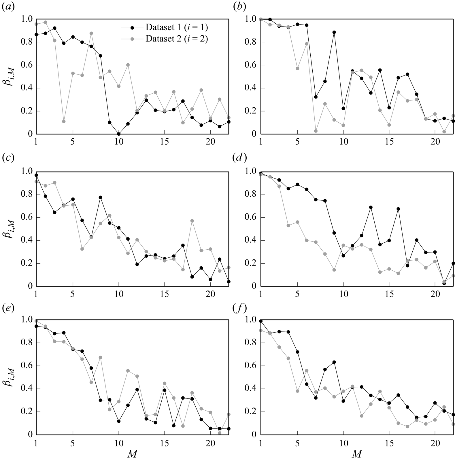
Figure 31. Convergence index  $\beta _{i,M}$ of the SPOD modes in the cases with (a,c,e)
  $AoA=7.5^{\circ }$ and (b,d,f)
  $AoA=10^{\circ }$. Here, only the zeroth, first and second frequencies are analysed due to their importance to the drag and lift coefficients stated in the main text.


 Open access