1 INTRODUCTION
Protoplanetary disks are both a by-product of star formation and the building blocks of planetary systems. Formed by gas and dust in an initial proportion of 100:1 (Bohlin, Savage, & Drake Reference Bohlin, Savage and Drake1978; Savage & Mathis Reference Savage and Mathis1979), their structure and evolution is driven by several interrelated physical mechanisms, including viscous evolution (Hartmann et al. Reference Hartmann, Calvet, Gullbring and D’Alessio1998), magnetospheric accretion (MA) (Koenigl Reference Königl1991), photoevaporation (Clarke, Gendrin, & Sotomayor Reference Clarke, Gendrin and Sotomayor2001), grain growth (Beckwith et al. Reference Beckwith, Sargent, Chini and Güsten1990; Miyake & Nakagawa Reference Miyake and Nakagawa1993), dust settling (D’Alessio et al. Reference D’Alessio, Calvet, Hartmann, Lizano and Cantó1999), and eventually, formation of planetary systems. Although assuming typical disk lifetimes of a few Myr (Sicilia-Aguilar et al. Reference Sicilia-Aguilar2006a; Hernández et al. Reference Hernández2007; Williams & Cieza Reference Williams and Cieza2011) is widely accepted, our understanding of the way disks evolve is still highly uncertain. Moreover, recent observations (e.g. HL Tau; Brogan et al. 2015) show that disk structure and evolution are intimately linked and need to be addressed together: Signs that were previously considered as unmistakable evidence of evolution (i.e. dust gaps) may be so common and appear so early, that they may be rather considered as typical disk structures.
One of the main problems in understanding disks is that the observable footprints of the diverse disk physics are highly degenerated, especially, when the available observations span few wavelengths, or are spatially unresolved. Different observations trace different parts of the disk, which is an additional difficulty for their interpretation. In addition, disks are physically situated somewhere between stellar atmospheres and molecular clouds, concerning densities and temperatures. Densities in disks span at least 10 orders of magnitude, and temperatures range from about 10 to 10 000 K, so even well-tested theories cannot be easily applied. This is why there is no alternative to the analysis of multi-wavelength, multi-telescope data.
Protoplanetary disks and their evolution forming planets cannot be captured in their entirety by looking at details seen at a single wavelength. Multi-wavelength data can help breaking the degeneracies, but observing time and sensitivity constraints impose strong limitations on the disks that can be observed. Observers usually choose one of two directions: either studying one object in great detail, or studying statistically significant samples of disks at well-selected (usually unresolved) wavelengths. High-resolution observations of bright systems unveil the disk structure and are a key to demonstrate the kind of physical processes that we can expect in disks, but they only have access to a few, nearby, bright objects, which may not be representative of most disks, nor solar analogues. Statistically significant observations of large numbers of disks are needed to reveal the common trends and prevalence of different disk structures, together with the time evolution, although the lesser detail carries the risk of always leaving an underlying degeneracy and it also overlooks object-to-object differences.
Current instrumentation (including multi-object capabilities and higher sensitivity on space- and ground-based facilities) are eroding the separation between individual-system studies and statistically significant observations by improving detectability and time-efficiency, but observational communities are still often working apart. This paper aims to determine what can be done and what would be possible in the near future in terms of observing and understanding protoplanetary disks. The Disk Rosetta Stone involves observational decryption of disks: Sometimes we observe the same phenomenon, but use different ‘languages’ (different wavelengths) to explore the physics. The apparently disconnected observations are part of the bigger picture (Figure 1).
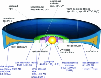
Figure 1. A cartoon of the observations and the parts of the disk that they trace, taking as example a young solar analogue. Although observations trace very different regions and processes in the disk, we need to keep in mind that they are all connected through the disk itself. Note that the complexity of the disk is highly reduced for clarity (for instance, not all the tracers become optically thick at the same location/depth). For a similar figure regarding the phyiscal processes, see Haworth et al. (Reference Haworth2016), Figure 1. Not to scale.
By putting together our observational knowledge, we present a common effort to trace the structure and evolution of protoplanetary disks using available telescopes and instrumentation, and discuss how new observing possibilities can be applied in the future to resolve the physics and structure of protoplanetary disks around T Tauri stars (TTS) and Herbig AeBe (HAeBe) stars. This paper concentrates on some of the most accessible, powerful, and complementary observational techniques currently available. It is thus not complete regarding all possible observations, it does not include future facilities, and it also does not discuss disk chemistry, which would require another paper by itself. We also limit our study to disks around Class II objects, leaving aside Class 0/I disks and post-processed, debris disks. Born at the ‘Protoplanetary Discussions’ in Edinburgh, 2016, this paper complements, from the observational point of view, the discussions that also gave rise to Haworth et al. (Reference Haworth2016) from the theoretical side. Section 2 discusses the significance and power of the measurements of the inner disk radius. Section 3 deals with holes and gaps in disks, their detectability, and their implications for disk evolution. The tracers of disk mass are explored in Section 4. Mass accretion is discussed in Section 5. Variable phenomena, time-dependent processes, and disk dynamics are presented in Section 6. Finally, we include a discussion on the complementarity and power of the mentioned combined techniques in Section 7 and our conclusions in Section 8.
2 MEASURING THE INNER DISK RADIUS
The first evidence of protoplanetary disks surrounding young stars came from IR excesses, together with observations of accretion and winds (e.g. Strom et al. Reference Strom, Strom, Edwards, Cabrit and Skrutskie1989). Given the wavelengths used in ground-based observations, most of the emission in the near-IR (NIR) originates in the disk inner rim, being dominated by dust at the dust sublimation radius (T ~ 1 500 K). The higher densities and shorter orbital periods in the innermost disk led to the prediction of inside-out disk dispersal (Hayashi, Nakazawa, & Nakagawa Reference Hayashi, Nakazawa, Nakagawa, Black and Matthews1985), later confirmed by the first observations of ‘transition disks’, presumed to be in a stage between disked and diskless stars, where the inner disk rim is larger than the dust sublimation radius (Strom et al. Reference Strom, Strom, Edwards, Cabrit and Skrutskie1989; Skrutskie et al. Reference Skrutskie, Dutkevitch, Strom, Edwards and Strom1990).
The inner disk, considered as the radial region inwards of ~ 10–20 AU that produces substantial emission in the NIR (in both gas and continuum), is a key region for the formation of habitable planetary systems, and for Solar Systems analogues. The large majority of exoplanets discovered to date have semi-major axes within ≈ 10 AU, making this disk region essential for the interpretation of exoplanet data.
While the inner dusty disk radius is physically set by the sublimation of dust grains at high temperatures (Section 2.2), other processes are expected to take over with time (e.g. grain growth, photo-evaporation, pebble/planetesimal/planet formation), pushing it to larger disk radii. The gaseous part of the disk can extend down to the corotation radius or the stellar magnetosphere (a few stellar radii in size), although depending on the temperature and density, the gas can be molecular or atomic. The hotter inner disk region is a key to understand the onset of disk dispersal through inner gaps in the gas and dust radial distributions. We put special emphasis on determining the ‘inner disk radius’ to constrain the disk evolutionary stage, noting that the radius depends on the tracer (gas, dust) used.
NIR and mid-IR (MIR) observations (1–30 μm) are very sensitive to dust close to the star, due to the large range of temperatures that produce substantial emission at these wavelengths (ranging from the dust sublimation temperature, ~ 1 500 to ~ 150 K), and to the large range of dust grain sizes that can produce the excess emission( ~ 0.1μm to ~ 20μm; Miyake & Nakagawa Reference Miyake and Nakagawa1993). Hot molecular line observations (e.g. CO, H2) trace the warm molecular layers in the disk.
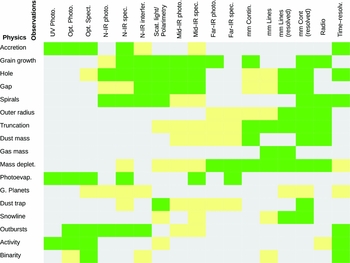
Figure 2 summarises the parts of the disk that can be detected in gas and dust with various techniques. The detectability depends on instrumental capabilities: maximum resolution with ALMAFootnote 1 , limiting magnitudes for SPHEREFootnote 2 , and MIDIFootnote 3 . We also assume that the disk is massive and bright enough, on the temperature of the gas or dust in the region. Since the dependency of the temperature with the radius is very complex (needs to take into account the density, grain sizes, chemistry, structure of the emitting region, scale height, plus potential heating mechanisms in addition to the central star), we take a simple approach where the temperature at each radii is assumed to be black-body-like and result from reprocessed star light alone. Although highly simplified, this figure reveals the main problem when measuring the inner disk rim: Different tracers are not sensitive to the same disk components, and can potentially produce very different results that need to be compared with care.
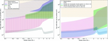
Figure 2. Disk radii that are accessible by different techniques tracing dust (left) and gas (right), for stars with different masses. The figure shows the regions where different methods overlap and what they cannot trace. Left: Detectable dust inner disk vs. stellar mass, as it can be observed at different wavelengths for an object at 140 pc distance. Resolved and unresolved observations are included. For unresolved observations, the detectability depends on the inner rim temperature, and is subject to model fitting (e.g. SED fitting), so the diagram shows the radii at which dust emission of larger than 15% over the photospheric levels can be detected. The lower edge of the observations correspond to the dust destruction radius (T ~ 1 500 K). For comparison, a stellar magnetosphere (between 4–8 Rstar) is also displayed. Right: Detectable gaseous inner disk vs. stellar mass, as it can be probed by different techniques. Note that for gas detetion, there is a distinction between atomic gas tracers and molecular gas. Beyond an approximate temperature of ~ 2 700 K, the gas is mostly atomic, although molecular gas can be found up to temperatures ~ 5 000 K, depending on density (Ilee et al. Reference Ilee2014). The CO gas will produce a substantial emission at temperatures > 300 K (Carmona et al. 2016), although detection may depend on the disk’s area. Also, note that ALMA gas observations at very high resolution are strongly limited by sensitivity, so most systems are not expected to be detectable as they do not have enough cold gas so far in.
Here, we consider the inner disk radius (or inner radial extent of the disk) as the radius closer to the central star where dust and molecular gas can survive and can be observed (the limits of this definition are discussed in each section below). In the following Sections, we discuss observations of the inner disk radius of dust and gas and how the dust sublimation radius (Rsubl) provides the reference to study the onset and evolution of inner disk dust gaps. We discuss first dust observations of Rin, dust, then molecular gas observations of Rin, CO and the picture emerging from combining the two.
2.1. Unresolved observations of the inner dusty disk
NIR observations were the basis of the first estimates of disk lifetimes (Haisch, Lada, & Lada Reference Haisch, Lada and Lada2001). With the advent of the Spitzer Space Telescope, large samples covering most of the disks and diskless populations in clusters, extended our knowledge of the dusty inner rim over several AU (see Figure 2). Spitzer data allowed to conduct statistical studies in disk evolution, including ‘transition disks’ (e.g. Sicilia-Aguilar et al. Reference Sicilia-Aguilar2006a; Najita, Strom, & Muzerolle Reference Najita, Strom and Muzerolle2007; Espaillat et al. Reference Espaillat2012). Despite being unresolved, the number of disks observed during the Spitzer cold mission is so overwhelming, that the statistical constraints on disk properties (including the presence of inner holes and gaps) and their lifetimes have provided one of the most complete and general views about the typical structures, dispersal paths, and lifetimes for the disks around solar- and late-type stars (Hartmann et al. Reference Hartmann, Megeath, Allen, Luhman, Calvet, D’Alessio, Franco-Hernández and Fazio2005; Megeath et al. Reference Megeath, Hartmann, Luhman and Fazio2005; Lada et al. Reference Lada2006; Sicilia-Aguilar et al. Reference Sicilia-Aguilar2006a; Hernández et al. Reference Hernández2007, amongst many others). Such unresolved observations are particularly important to study disk dispersal in solar analogues, since dispersing disks around low- and solar-mass stars are very often too faint to be resolved otherwise.
Silicate emission is another tracer of the dust grains in the warm disk atmosphere and a signature of the vertical temperature structure in the disk (Calvet et al. Reference Calvet1992; D’Alessio et al. Reference D’Alessio, Calvet, Hartmann, Franco-Hernández and Servín2006). Although for most disks, the silicate observations are unresolved, it is possible to obtain spatially resolved silicate data (Van Boekel et al. Reference Van Boekel, Waters, Dominik, Dullemond, Tielens and de Koter2004; Juhász et al. Reference Juhász2012). Partly observable from the ground, it was efficiently observed for large samples of objects thanks to Spitzer/IRS, allowing to study the disk mineralogy in a statistically significant way. Even though the silicate emission does not provide information on the global grain properties in the disk, it is a sign of grain processing, heating, mixing, and transport in the disk. Dust processing happens in all protoplanetary disks, ranging from HAeBe (Meeus et al. Reference Meeus, Waters, Bouwman, van denAncker, Waelkens and Malfait2001; Bouwman et al. Reference Bouwman, Meeus, de Koter, Hony, Dominik and Waters2001; Van Boekel et al. Reference Van Boekel2005) to brown dwarf (BD) disks (Apai et al. Reference Apai, Pascucci, Bouwman, Natta, Henning and Dullemond2005; Ricci et al. Reference Ricci2014). Crystalline silicates are not found in the ISM (Kemper, Vriend, & Tielens Reference Kemper, Vriend and Tielens2004) and require very specific conditions for their formation. Thus, the mass fraction of crystals and stochiometry of the silicates can be used to trace the physical conditions in the disk when the material formed, including the temperature, initial chemical composition, grain sizes, velocities, and the time frame for annealing, considering the different chemical reactions that give rise to the production of different silicate components (e.g. silica, forsterite, enstatite; Bouwman et al. Reference Bouwman, Meeus, de Koter, Hony, Dominik and Waters2001; Henning Reference Henning2010). The formation of a silicate feature is also strongly connected to the disk structure, so the size of the emitting region can be estimated even in unresolved observations, considering the strength of the emission in different silicate bands (Kessler-Silacci et al. Reference Kessler-Silacci2007; Bouwman et al. Reference Bouwman2008; Juhász et al. Reference Juhász2010).
The silicate feature is optically thin, which allows to estimate the dust mass and composition fraction in the outer disk layers and, comparing to the continuum, to discern the presence of gaps and holes (Bouwman et al. Reference Bouwman2010) and the presence of large ( ~ 10 μm) grains in the disk atmosphere, used to constrain turbulence and settling (Sicilia-Aguilar et al. Reference Sicilia-Aguilar2007; Pascucci et al. Reference Pascucci, Apai, Luhman, Henning, Bouwman, Lahuis and Natta2009). The lack of strong amorphous silicate features in intermediate-aged disks around M-type stars is interpreted as a sign of grain growth and settling in the innermost disk, which dominates the 10 μm emission (Sicilia-Aguilar et al. Reference Sicilia-Aguilar2007). The lack of trends between crystallinity and other disk and stellar properties (Watson et al. Reference Watson2009; Sicilia-Aguilar et al. Reference Sicilia-Aguilar2007, Reference Sicilia-Aguilar2011) suggests that their formation depends on many factors, including rapid creation and mixing of crystalline silicates on timescales much shorter than those of disk evolution (Ábrahám et al. Reference Ábrahám2009; Juhász et al. Reference Juhász2012). Finally, crystalline silicates could be used as indirect signatures of the presence of planets, related to heating by shocks (Desch et al. Reference Desch, Ciesla, Hood and Nakamoto2005; Bouwman et al. Reference Bouwman2010).
2.2. Inner extent of dust in disks
Although modelling spatially unresolved spectral energy distributions (SED) provides some constraints on the inner disk radius, the most accurate measurements of Rin, dust come from spatially resolved interferometric observations of NIR dust emission. These measurements showed that the spatial extent of the hottest dust in disks were not consistent with disk models extending up to the star, and were found to correlate with the squared root of the stellar luminosity as Rin, dust ∝ L1/2 ⋆ (Monnier & Millan-Gabet Reference Monnier and Millan-Gabet2002; Dullemond & Monnier Reference Dullemond and Monnier2010). This correlation was readily explained with the existence of a dust sublimation front at temperatures of 1300–1500K: Most of the NIR dust emission is emitted by a disk rim located at the dust sublimation front (Natta et al. Reference Natta2001; Dullemond, Dominik, & Natta Reference Dullemond, Dominik and Natta2001). The gas inside this rim must be radially optically thin enough to allow a direct irradiation of the rim. More physical models of the rim were proposed, including the physics of dust sublimation (Isella & Natta Reference Isella and Natta2005), multiple dust species and full radiative transfer (Kama, Min, & Dominik Reference Kama, Min and Dominik2009) and detailed hydrodynamics (Flock et al. Reference Flock, Fromang, Turner and Benisty2016). The radial location of the dust rim can provide constraints on the inner disk dust surface density, size distribution, and material through an analytical formula or through detailed models (Kama et al. Reference Kama, Min and Dominik2009; Flock et al. Reference Flock, Fromang, Turner and Benisty2016).
The advent of new instruments at VLTI, such as AMBER and PIONIER, and the use of very long baselines (CHARA), enabled detailed modelling of multi-wavelength observations. These showed that additional material (gas or refractory species) could contribute significantly to the NIR excess (Kraus et al. Reference Kraus2008; Tannirkulam, Harries, & Monnier Reference Tannirkulam, Harries and Monnier2007; Benisty et al. Reference Benisty2010a). Multi-wavelength observations revealed systems with cleared regions (Olofsson et al. Reference Olofsson2011, Reference Olofsson2013; Tatulli et al. Reference Tatulli2011; Matter et al. Reference Matter2014), and optically thin material located inside the gap (Kraus et al. Reference Kraus2012). With a larger number of observations available, the images of the first AU could be reconstructed, unveiling a complex morphology (Renard et al. Reference Renard, Malbet, Benisty, Thiébaut and Berger2010; Benisty et al. Reference Benisty, Tatulli, Ménard and Swain2010b). Although the most detailed studies were focussed on a small samples, recent homogeneous PIONIER observations of HAeBe stars found that very few objects show well-resolved puffed-up rims, so that the sublimation front is rather smooth and not a sharp transition (Lazareff et al. submitted). Large-scale emission, contributing to lower visibilities at short baselines, might indicate cavity walls. Similar findings were derived from a statistical analysis of MIR observations (Millan-Gabet et al. Reference Millan-Gabet2016).
As a cautionary note, resolved observations are subject to interpretation through models that depend on the dust composition and size distribution, on the structure of the rim, on the dust density, and on the temperature. The dust composition and size affects the dust opacity, which controls the local temperature (see Section 7). Observations of different objects, including those with and without inner holes, and combination with multi-wavelength observations to track the gas content and the extended disk structure are a key to put these observations into a broader context.
2.3. Inner extent of molecular gas in disks
Similarly to the hottest dust in the inner disk, the hottest (and innermost, in terms of disk radii) molecular gas emission typically peaks in the NIR with ro-vibrational branches at 2–5 μm (e.g. Figure 7 in Salyk et al. Reference Salyk, Blake, Boogert and Brown2009), or in the UV at 1 300–1 700 Å (France et al. Reference France2011, Reference France2012). With due differences, spatial information on the gas-emitting region can be obtained with interferometry (Eisner et al. Reference Eisner2010; Eisner, Hillenbrand, & Stone Reference Eisner, Hillenbrand and Stone2014), spectro-astrometry (Pontoppidan et al. Reference Pontoppidan2008; Pontoppidan, Blake, & Smette Reference Pontoppidan, Blake and Smette2011; Brittain, Najita, & Carr Reference Brittain, Najita and Carr2015), position-velocity diagrams (Goto et al. Reference Goto2006; Brittain, Najita, & Carr Reference Brittain, Najita and Carr2009; van der Plas et al. Reference van der Plas2009; Carmona et al. Reference Carmona2011), and with high-dispersion spectrographs through fully spectrally resolved velocity profiles (Brown et al. Reference Brown2013; Banzatti & Pontoppidan Reference Banzatti and Pontoppidan2015). For optically thin lines, the strength of NIR gas emission lines is linked to the column density, temperature, and excitation conditions of hot gas in the inner disk. Optically thick lines trace the temperature in the emitting region, which has a complex dependency on the gas density.
The emission from two molecules, H2 and CO, is especially suited to trace the innermost disk region where molecular gas can survive: They are abundant (being made by the most abundant atoms), they share a similarly high thermal dissociation temperature ( ~ 4500 K) and they can also self-shield to dissociating UV radiation to some extent (Bruderer Reference Bruderer2013a; see Section 2.4).
The NIR CO fundamental ro-vibrational lines are good tracers of the gas in the inner disk because their energy levels are sufficiently populated at the temperatures found at 0.1–10 AU and because their Einstein A coefficients are large, making them much stronger than the NIR H2 lines (e.g. Carmona et al. Reference Carmona2008; Bitner et al. Reference Bitner2008), which lack a permanent dipole moment. As the CO emission becomes optically thick at low column densities (NCO ~ 1016 cm−2 or NH ~ 1020 cm−2), strong lines are formed even in the upper regions where the dust is optically thin. The CO overtone needs higher column densities and temperatures than CO ro-vibrational to be excited (NCO ~ 5 × 1020 cm−2, T > 1 700 K; Bik & Thi 2004), being mostly observed in massive young stars.
UV pumping triggers H2 emission at 2.12 μm, which can be detected up to 150 AU if the disk is warm and flared (e.g. Carmona et al. Reference Carmona2011). H2 also has stronger fluorescent transitions (excited by Lyα photons) in the UV that been observed with IUE and HST wavelengths and that are also detectable for CTTS and transition disks (Valenti et al. Reference Valenti, Fallon and Johns-Krull2003; Hoadley et al. Reference Hoadley, France, Alexander, McJunkin and Schneider2015). The main limitation for these observations are the brightness of the target and whether there is still enough gas at a high enough temperature, to produce substantial NIR emission. This poses a general outer limit of ≈ 20 AU to the disk regions that can be studied in the thermal NIR, as well as sensitivity limits of the individual techniques. All considered to date, high-dispersion spectroscopy of NIR CO emission has provided the largest and most informative dataset of molecular gas observations in inner disks (Brown et al. Reference Brown2013; Banzatti & Pontoppidan Reference Banzatti and Pontoppidan2015).
High-dispersion spectroscopy provides a way to characterise the emitting region of gas in disks even at scales not directly spatially resolvable. This is achieved by modelling velocity-resolved line profiles broadened by Keplerian rotation in the disk. The observed velocities depend on Kepler’s law and on the inclination angle, so that emission from smaller orbital radii has higher velocity shifts. The observed line profiles therefore provide measurements of the disk radii where CO is emitting, being ‘spatially-resolved’ through the velocity shifts. To fully spectrally resolve a line from a ≲ 10 AU disk radii, a resolving power of at least 25 000 is required, depending on the disk inclination. In the case of NIR observations, this is currently achieved by high-resolution slit spectrographs such as CRIRES at the ESO-VLT, iSHELL on the IRTF, NIRSPEC at Keck, and IRCS at Subaru. This technique has proven to be efficient in surveys of velocity-resolved CO emission, especially with the advent of CRIRES (e.g. Pontoppidan et al. Reference Pontoppidan, Blake and Smette2011; Brown et al. Reference Brown2013; Banzatti & Pontoppidan Reference Banzatti and Pontoppidan2015). It allows us to study a radial region between 0.05–20 AU in disks around stellar masses ≳ 0.3 M⊙, based on flux sensitivity limits of CRIRES of ≈ 2–10−16 erg cm−2 s−1 for an unresolved line with resolution 3.3 km s−1 and a typical line width of 10 km s−1. The minimum column density depends on the assumed gas temperature, the size of the emitting region, and the disk inclination. From observations of HD 139614 (Carmona et al. 2016), the minimum column density detectable at 3σ level was NH = 5 × 1019 cm−2 (NCO = 5 × 1015 cm−2) for a disk of gas between 0.1–1.0 AU at T = 675–1 500 K inclined 20° around a 1.7 M⊙ star.
If the emitting region is beyond 10–30 AU in disks at 120–140 pc, CO emission lines can be directly spatially resolved in position-velocity diagrams (Goto et al. Reference Goto2006; Brittain et al. Reference Brittain, Najita and Carr2009; van der Plas et al. Reference van der Plas2009; Carmona et al. Reference Carmona2011). If the emitting region is < 10 AU, information on the spatial scales can be retrieved from the spectroastrometry signature of the line profiles in the 2D spectrum (e.g. Pontoppidan et al. Reference Pontoppidan, Blake and Smette2011; Brown et al. Reference Brown2013; van der Plas et al. Reference van der Plas, van den Ancker, Waters and Dominik2015). Spectroastrometry essentially measures the shift on the centre of the point spread function (PSF) at the position of the emission lines in the 2D spectrum. As the centre of the PSF can be measured with an accuracy of the order of 1/10 of a pixel with CRIRES (with the assistance of adaptive optics), spatial information can be retrieved on spatial scales of the order of 0.01 arcsec (= 1 AU at 100 pc), for bright enough sources. This technique has been successfully implemented in a dozen of disks so far (Pontoppidan et al. Reference Pontoppidan2008, Reference Pontoppidan, Blake and Smette2011; Brittain et al. Reference Brittain, Najita and Carr2015). Its success depends, amongst other things, on the disk inclination and on reaching a good S/N, which strongly limits the observations of faint and low-mass disks. NIR interferometry has been used to detect CO emission at 2.3 μm at disk radii of < 2 AU (Eisner et al. Reference Eisner2010, Reference Eisner, Hillenbrand and Stone2014). The low detection rates with this technique suggested that the most effective range to study CO gas in inner disks is at 4.6–5 μm, where the emission is more frequently found, also for low-mass stars (Goto et al. Reference Goto2006; Brown et al. Reference Brown2013; Banzatti & Pontoppidan Reference Banzatti and Pontoppidan2015).
All the NIR observing techniques mentioned above provide spatial information on CO emission in the inner disks. As they probe the hottest molecular gas, the spatial information is usually regarded as a measurement of the smallest stellocentric distance where the molecular gas survives, which we call Rin, CO as being based mostly on observations of CO. These measurements have a high potential to constrain disk structure and evolution, as we will discuss later. In velocity-resolved observations, the velocity at the half width at half maximum (HWHM) of the line provides a measurement of the disk radius close to where the peak line flux is emitted. At smaller disk radii, less than 10% of the line flux is typically emitted, with slight differences depending on how steep line wings are (Banzatti & Pontoppidan Reference Banzatti and Pontoppidan2015). In spectroastrometry, Rin, CO is usually taken at the peak of the spectro-astrometric signal, which corresponds to the disk radius that contributes most to the emission (Pontoppidan et al. Reference Pontoppidan2008, Reference Pontoppidan, Blake and Smette2011). Models show that Rin, CO from CO ro-vibrational emission corresponds to the location of the maximum CO intensity when a power law for the intensity, or a power-law column density and temperature profiles are assumed. It effectively corresponds to the disk radius where CO emission becomes optically thick. From Rin, CO inward to the star, the column density of CO decreases, so the value depends on how the temperature increases at lower radii. For a detection, the decline on surface density should (combined with the decrease on solid angle) be faster that the increase on temperature.
As being based on molecular gas, Rin, CO does not imply that no gas is present closer to the star. Atomic gas usually extends inward to the magnetospheric radius to feed stellar accretion, and it is often much easier to detect accretion than molecular gas, especially in low-mass disks (see Section 5).
2.4. Rin > Rsubl: the onset of inner disk gaps?
Given that the dust dominates the opacity and controls the amount of UV radiation penetrating the disk, the survival of molecular gas is expected to be linked to the presence of shielding dust. We would thus expect Rin, dust and Rin, CO to agree with each other in disks, but CO is able to self-shield against UV radiation, surviving down to very low amounts of gas mass even in the total absence of dust grains (e.g. 12CO self-shields at NCO ~ 1015 cm−2, corresponding to NH ~ 1019cm−2, assuming standard abundances; van Dishoeck & Black Reference van Dishoeck and Black1988; Bruderer 2013b). Although Rin, dust is set by the dust sublimation temperature( ~ 1500 K), Rin, CO may be smaller than expected from the thermal dissociation temperature of CO (4 500 K) due to self-shielding. If Rin, dust is larger than Rsubl,, the dust is removed by means other than dust sublimation. In this case, if Rin, CO still matches Rin, dust, it means that whatever process is removing dust it is also removing CO gas, because otherwise CO gas should self-shield and exist down to < Rsubl,. Therefore, comparison of measured Rin, dust and Rin, CO to Rsubl, can help to understand the physics and processes that regulate the inner disk structure.
In Figure 3, we show measurements of Rin, dust from IR interferometry (Anthonioz et al. Reference Anthonioz2015; Menu et al. 2015) and of Rin, CO from IR spectroscopy of CO gas (Banzatti & Pontoppidan Reference Banzatti and Pontoppidan2015), as compared to a simplified parameterisation of Rsubl, (Dullemond & Monnier Reference Dullemond and Monnier2010, Salyk et al. 2011). The two probes of Rin agree with each other and with Rsubl, in most disks around stars with masses < 1.5 M⊙, supporting the idea that CO survives where dust survives, and that dust survives until it is destroyed by the high temperatures close to the star. Rin, CO is much larger than Rsubl, in some disks, though, and notably some of them are known to be ‘transitional’ disks from observations of the inner dust (e.g. TWHya). Remarkably, for stellar masses of > 1.5 M⊙, Rsubl, is smaller than both Rin, dust and Rin, CO in the vast majority of disks. This has been recently interpreted as evidence that most of these disks are forming inner gas and dust holes by means different than dust sublimation (Maaskant et al. Reference Maaskant2013; Banzatti & Pontoppidan Reference Banzatti and Pontoppidan2015; Menu et al. Reference Menu2015b).
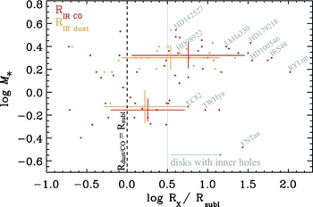
Figure 3. Measurements of RIR, dust from IR interferometry (orange points, from Anthonioz et al. Reference Anthonioz2015; Menu et al. Reference Menu2015b) and of RIR, CO from IR spectroscopy of CO gas (red points, from Banzatti & Pontoppidan Reference Banzatti and Pontoppidan2015). The dust/CO radii (R X ) are normalised to the dust sublimation radii Rsubl, expected from models. Large crosses show median values and median absolute deviations for two stellar mass bins.
The combination of observations at different wavelengths can thus help to explore the various possibilities of disk dispersal in the inside-out scenario to understand the physics and connections between gas and dust, and the process of accretion and transport in the innermost disk, all highly relevant for the formation of terrestrial planets and Solar Systems analogues.
3 IMAGING DISK GAPS AND LARGE-SCALE ASYMMETRIES
Large-scale asymmetries are increasingly attracting the attention of the disk and planet communities, thanks to the recent spatially resolved images of structures in disks. These observations have revealed that deviations from a continuous radial or azimuthal distributions are common in protoplanetary disks. The most typical radial discontinuities are disk ‘gaps’, ‘holes’, and ‘rings’. The term ‘cavity’ has also been frequently used to define a significant depletion of material occurring in the inner tens of AU, regardless of the presence of substantial material close to the star. In this section, we define gap and ring as any azimuthally symmetric deficit and enhancement in the disk brightness, respectively. In most cases (but not all), these deficits and enhancements are to be ascribed to a real depletion or concentration of material. Azimuthal discontinuities like lopsided rings or spirals are also often observed in disks, with the former structures being common in millimetre imaging and the latter in the visible/NIR scattered light. We note that the disk regions with mass depletion are usually not completely devoid of material (i.e. gas is often observed inside dust gaps). Gaps and holes observed with different tracers look different and do not always agree because individual gas and dust tracers have strong restrictions on the temperature, density, and grain size of the material they can detect. Some disks that show clear holes in mm interferometry show no holes in scattered-light imaging, and IR dust and gas observations find that these holes are not void regions but still host disk material. The reconciliation of these observations is currently a necessity, because while the incorrect use of definitions may produce confusion, the combination of different tracers bears the power to clarify the origin of disk gaps/holes and their link to disk evolution.
To date, it is still unclear how disk dispersal in the inside-out scenario may be linked to the rapidly increasing number of spatially resolved observations of gaps and holes, spirals, and other radially or azimuthally asymmetric features detected at radii > 10 AU. The concept of disks that are ‘primordial’ and disks that are ‘in transition’ may need to be revisited on the basis of new evidence from the growing number of spatially resolved observations, which shows that disks may have structures previously attributed to evolution at phases much earlier than previously expected (e.g. ALMA image of HLTau).
Clarifying the link between the disk gaps observed on small and large scales and the global disk structure is essential to understand disk evolution (e.g. Owen Reference Owen2016). The growing number of observations that probe disk material within or beyond 10 AU starts now to provide grounds towards a unified picture of disk evolution and dispersal. For instance, ALMA can provide spatially resolved images only down to disk radii ≳ 3 AU at 120–140 pc (or ≳ 30 AU in star-forming regions at 1 kpc)Footnote 4 . ALMA is also not optimal to observe disk gas at ≲ 10 AU due to a combination of angular and spectral sensitivity and the fact that the hot gas emits strongly in the IR, but not at mm wavelengths. On the other hand, ro-vibrational CO emission at NIR wavelengths is a good tracer of disk structure and gaps at 0.05–20 AU (Salyk et al. 2011, Banzatti & Pontoppidan Reference Banzatti and Pontoppidan2015), and NIR dust emission probes a similar region (see Section 2), providing overlap and complementarity to the disk region probed by mm interferometers. A global understanding of gaps therefore requires a combination of observations at different wavelengths to probe disk radii from the smallest to the largest distances from the star in both gas and dust.
In this section, we explore how different imaging techniques see gaps and asymmetries in disks (specifically mm interferometry and optical/IR scattered light imaging), and describe their limits, ranges, and degeneracies.
3.1. Millimetre continuum interferometry observations
Whereas dust gaps in disks were traditionally identified through a dip in the MIR part of their SED due to the deficit of warm dust (e.g. Strom et al. Reference Strom, Strom, Edwards, Cabrit and Skrutskie1989; Forrest et al. Reference Forrest2004; Calvet et al. Reference Calvet2005; Brown et al. Reference Brown2007), their presence was confirmed through (sub)millimetre interferometric imaging at subarcsecond resolution, using e.g. the SubMillimeter Array (SMA), Plateau de Bure Interferometer (PdBI), and Combined Array for Research in Millimeter-wave Astronomy (CARMA). The millimetre continuum images revealed that dust was indeed depleted from the inner tens of AU of the disk, showing ring-like outer disk structures (e.g. Piétu et al. Reference Piétu, Dutrey, Guilloteau, Chapillon and Pety2006; Dutrey et al. Reference Dutrey2008; Hughes et al. Reference Hughes2009; Brown et al. Reference Brown2009; Isella et al. Reference Isella, Natta, Wilner, Carpenter and Testi2010; Andrews et al. Reference Andrews2011b; see review in Williams & Cieza Reference Williams and Cieza2011). Interestingly, some large mm-dust cavities were found in disks without a clear deficit in their SED, e.g. MWC758, UX Tau A, and WSB 60, possibly due to vertical structure and small/large dust grain segregation (Andrews et al. Reference Andrews2011b).
The image quality of these pioneering interferometers was rather low, due to the small number of antennas, resulting in low u,v-coverage and S/N (typically 10–20 peak S/N ratios). The image results from the Fourier transform of the observed visibilities, using a deconvolution algorithm (cleaning) to suppress the side lobes. Interpretation of these images thus has to be done with care, as the deconvolution process generally does not result in a beam-convolved image, but rather the best attempt of the algorithm to deconvolve the data with incomplete u,v-sampling. The visibility data can be represented in a real and an imaginary component as function of baseline (u,v-distance), usually deprojected along the position angle and inclination of the disk (Berger & Segransan Reference Berger and Segransan2007). The real component represents the radial variations, and for a ring-like structure, it shows an oscillation pattern (following a Bessel function), where the first ‘null’ is a measure of the cavity size (Hughes et al. Reference Hughes2007). Emission in the imaginary component indicates azimuthal asymmetries along the ring: Zero emission indicates an axisymmetric disk. The real and imaginary components are measured with respect to the phase centre, the centre of the disk, so an offset will result in non-zero imaginary emission.
Interpretation of the dust continuum images is usually done by fitting the visibilities (in the u,v-plane) with a radiative transfer model. Typical dust models include a dust surface density profile Σ(r), following a power-law with or without exponential tail, and an inner cut-off at the dust cavity radius. This cut-off is usually taken to be sharp, to simplify the fitting and limit the parameter space, although this is generally considered to be unphysicalFootnote 5 . When near infrared excess is measured in the SED, an inner disk is often added by setting Σ(r) to non-zero between the dust sublimation radius and an arbitrary inner disk size (typically 1–10 AU). The inner disk may cast shadows on the gap edge, so this is a crucial part of the interpretation of mm data. As azimuthal asymmetries were usually not significant, a simple assumption of an axisymmetric disk was used, with zero imaginary emission.
The huge increase of sensitivity and u,v-coverage by ALMA has resulted in many high quality images of disk dust gaps at 0.2–0.3 arcsec resolution (e.g. van Dishoeck et al. Reference van Dishoeck, van der Marel, Bruderer, Pinilla, Iono, Tatematsu, Wootten and Testi2015). The high S/N (typically > 100) leaves no doubt about the azimuthally asymmetric nature of some of these disks. The most extreme examples are Oph IRS 48 (van der Marel et al. Reference van der Marel2013) and HD 142527 (Casassus et al. Reference Casassus2013; Fukagawa et al. Reference Fukagawa2013) with contrasts ~ 30–130. Minor azimuthal asymmetries with contrasts of ≲ 2 appear in SR 21 and HD 135344B (Pérez et al. Reference Pérez, Isella, Carpenter and Chandler2014; Pinilla et al. Reference Pinilla2015a). Several clearly axisymmetric dust rings are also found (e.g. Zhang et al. Reference Zhang, Isella, Carpenter and Blake2014; Walsh et al. Reference Walsh2014; van der Marel et al. Reference van der Marel, van Dishoeck, Bruderer, Pérez and Isella2015b, Reference van der Marel2016; Canovas et al. Reference Canovas2016). These structures can be understood in the context of mm-dust trapping in gas pressure bumps (e.g. Whipple Reference Whipple and Elvius1972; Pinilla, Benisty, & Birnstiel Reference Pinilla, Benisty and Birnstiel2012). This is supported by the segregation of small dust grains as seen in scattered light, where observations reveal no or smaller gaps (e.g. Garufi et al. Reference Garufi2013), and the presence of gas inside the dust cavity as shown by ALMA CO observations (e.g. Pontoppidan et al. Reference Pontoppidan2008; Bruderer et al. Reference Bruderer, van der Marel, van Dishoeck and van Kempen2014; Zhang et al. Reference Zhang, Isella, Carpenter and Blake2014; Perez et al. Reference Perez2015; Banzatti & Pontoppidan Reference Banzatti and Pontoppidan2015; van der Marel et al. Reference van der Marel, van Dishoeck, Bruderer, Pérez and Isella2015b, Reference van der Marel2016; Canovas et al. Reference Canovas2016). CO intensity maps (integrated over velocity) can resolve the gas cavities directly at ~ 0.25 arcsec resolution, when their inner radius is large enough (several tens of AU). A quantitative analysis of these data indicates deep gas gaps, with density drops of several orders of magnitude, which are smaller than the dust gaps (van der Marel et al. Reference van der Marel2016 a). However, the amount of gas inside ~ 10 AU remains unconstrained, as the emission at this resolution is dominated by the edge of the gap. NIR observations (Section 2) provide more information about the presence of gas closer to the star. The dust asymmetries may result from azimuthal trapping in a vortex, as a result of Rossby Wave instability in the pressure bump (e.g. Barge & Sommeria Reference Barge and Sommeria1995; Birnstiel, Dullemond, & Pinilla Reference Birnstiel, Dullemond and Pinilla2013; Lyra & Lin Reference Lyra and Lin2013).
Considering the large parameter space and the high S/N, intensity profiles rather than full radiative transfer models are often used to fit these data, especially in azimuthally asymmetries (van der Marel et al. Reference van der Marel2013; Pérez et al. Reference Pérez, Isella, Carpenter and Chandler2014; Walsh et al. Reference Walsh2014; Pinilla et al. Reference Pinilla2015a; van der Marel et al. Reference van der Marel2015a). The edges are generally more consistent with a smooth ring (following a radial Gaussian) rather than a sharp cut-off (Andrews et al. Reference Andrews, Rosenfeld, Wilner and Bremer2011a). Observing the continuum at different wavelengths reveals a wavelength dependency of the cavity size through the shift of the null in the visibilities (e.g. Pinilla et al. Reference Pinilla2015a; van der Marel et al. Reference van der Marel, van Dishoeck, Bruderer, Pérez and Isella2015b) or as radial dependence of the spectral index α, with F mm ~ να (e.g. Wright et al. Reference Wright2015; Casassus et al. Reference Casassus2015; van der Marel et al. Reference van der Marel2015a), indicating that the larger dust grains are usually more concentrated.
As ALMA is reaching its full capacity, milliarcsecond observations have revealed a possibly different type of gaps in disks: Series of narrow bright and dark rings in the dust continuum of HL Tau and TW Hya (Brogan et al. 2015; Andrews et al. Reference Andrews2016), which are interpreted through a range of possibilities in the context of planet gaps, snowlines, magnetised disks, dust opacity effects, and sintering-induced dust rings (e.g. Dong, Zhu, & Whitney Reference Dong, Zhu and Whitney2015; Zhang, Blake, & Bergin Reference Zhang, Blake and Bergin2015; Banzatti et al. Reference Banzatti2015b; Flock et al. Reference Flock2015; Pinte et al. Reference Pinte2016; Okuzumi et al. Reference Okuzumi, Momose, Sirono, Kobayashi and Tanaka2016).
3.2. Scattered light observations
Scattered light observations in the visible and NIR probe the dust in the surface layers of the disk. At those wavelengths, a relatively small column density of dust is enough to attain a scattering optical depth of the order of unity. These observations mostly trace (sub-)micron sized grains, which are the dominant population of dust at the disk surface, as the strong coupling between small dust grains and gas attenuates their settling towards the midplane. To spatially resolve a disk in scattered light, high-contrast and high-resolution observations are needed. This has biased the sample of detected protoplanetary disks ( ~ 30) towards bright disks around HAeBe stars in the nearest star-forming regions (see Quanz Reference Quanz2015). The primary limit on the stellar brightness is dictated by the adaptive optics system, whereas large disk brightnesses are needed to obtain a relatively high contrast with the stellar luminosity.
Differential imaging techniques are used to overcome the large star-disk flux contrast at small angular separations. Post-processing PSF subtraction initiated the high-contrast imaging by means of coronagraphic Hubble Space Telescope (HST) observations (e.g. Grady et al. Reference Grady1999; Weinberger et al. Reference Weinberger1999). This technique is powerful to resolve the outer disk region, but limits the access to the inner ~ 1 arcsec because of the limited telescope size and the need for a coronagraphic mask. Ground-based facilities like the VLT and Gemini provide dedicated differential imaging instrumentation (e.g. Beuzit et al. Reference Beuzit2006; Macintosh et al. Reference Macintosh2008). Angular differential imaging (ADI) was developed for direct detection of companions, but it can be used for scattered light observations of disks. The principle of ADI is to keep the orientation of the telescope pupil fixed on the detector such that the field of view rotates around the target star. In this way, the disk signal rotates with respect to the quasi-static speckles and a reference PSF can be constructed from the target star itself (Marois et al. Reference Marois, Lafrenière, Doyon, Macintosh and Nadeau2006). This technique is particularly powerful for radially narrow disks, such as debris and edge-on disks (Milli et al. Reference Milli2012) but it may suffer from flux losses by self-subtraction in extended disks (Garufi et al. Reference Garufi2016). Polarimetric differential imaging (PDI) makes use of the polarising nature of dust grains by taking the difference of orthogonally polarised images which subtracts the unpolarised stellar halo and speckles (Canovas et al. Reference Canovas, Rodenhuis, Jeffers, Min and Keller2011; Avenhaus et al. Reference Avenhaus2014a, e.g.). Pioneering works were done by Kuhn, Potter, & Parise (Reference Kuhn, Potter and Parise2001) and Apai et al. (Reference Apai2004), while the first systematic census of protoplanetary disks in PDI was performed with Subaru/HiCIAO by the SEEDS consortium (e.g. Hashimoto et al. Reference Hashimoto2011; Kusakabe et al. Reference Kusakabe2012; Grady et al. Reference Grady2013).
The surface brightness of a disk in scattered light depends both on the disk structure and the scattering properties of the dust grains in the disk surface. For example, a local change in surface density or pressure scale height will affect the irradiation of the disk surface and the amount of light scattered into our line of sight. For inclined disks, the surface brightness is also determined by the dust properties because of the scattering angle dependence on the phase function and the degree of polarisation. Scattered light provides also insight into the dust properties in the disk surface through measurements of disk colour (e.g. Mulders et al. Reference Mulders, Min, Dominik, Debes and Schneider2013; Stolker et al. Reference Stolker2016) and phase function (Stolker et al. subm.). While small (compared to the observed wavelength) grains scatter isotropically, the phase function of larger grains has a forward scattering peak which can manifest itself as a brightness asymmetry of the near and far side of a disk (e.g. Mishchenko, Hovenier, & Travis Reference Mishchenko, Hovenier and Travis2000; Thalmann et al. Reference Thalmann2014). On the other hand, the degree of polarisation typically peaks around scattering angles of 90°, which is near the disk major axis (e.g. Hashimoto et al. Reference Hashimoto2012; Min et al. Reference Min, Rab, Woitke, Dominik and Ménard2016). The combined effect of disk structure, phase function, and degree of polarisation can make the interpretation of polarised surface brightness non-trivial: Disentangling the different effects may require radiative transfer modelling. Here, sub-millimetre observations can help to trace a complete picture of the distribution of small dust, large dust, and gas throughout a disk (see Section 7).
Several types of morphological features and brightness asymmetries have been detected in scattered light (e.g. Casassus Reference Casassus2016). Spiral arms have been observed in a number of transition disks (e.g. Muto et al. Reference Muto2012; Garufi et al. Reference Garufi2013; Wagner et al. Reference Wagner, Apai, Kasper and Robberto2015). Their origins are still debated due to our limited knowledge of their vertical structure, since in principle both global changes of the dust properties and small variations on the disk scale height may account for the observations. The observed spirals can be produced by various mechanisms, including planet/stellar interactions with the disk (e.g. Ogilvie & Lubow Reference Ogilvie and Lubow2002; Boss Reference Boss2006), gravitational instabilities (e.g. Cossins, Lodato, & Clarke Reference Cossins, Lodato and Clarke2009), and shadowing effects (Montesinos et al. Reference Montesinos2016). The visibility of a spiral density wave in scattered light depends on the strength of the temperature and/or surface density perturbation (Juhász et al. Reference Juhász2015). A massive planet can trigger both a primary and secondary spiral arms interior to its orbit (Dong et al. Reference Dong, Zhu, Rafikov and Stone2015), which resembles some of the observed spiral arms (e.g. Benisty et al. Reference Benisty2015).
Brightness asymmetries may also be related to global or local asymmetries in the disk structure. In some cases, a plausible connection between disk surface and midplane can be made when the asymmetry in scattered light and sub-mm dust continuum coincides (e.g. Garufi et al. Reference Garufi2013; Marino et al. Reference Marino2015).
Radial reductions in surface brightness are often interpreted as gaps (e.g. Quanz et al. Reference Quanz2013; Thalmann et al. Reference Thalmann2015; Rapson et al. Reference Rapson, Kastner, Millar-Blanchaer and Dong2015). Nevertheless, a decrease in the scattered light flux does not necessarily relate to a decrease in gas and/or dust surface density but could also be a shadowing effect (e.g. Siebenmorgen & Heymann Reference Siebenmorgen and Heymann2012; Garufi et al. Reference Garufi2014). Local shadowing effects have been detected on a few disks: For example, a warped inner disk (Marino, Perez, & Casassus Reference Marino, Perez and Casassus2015) can produce azimuthal surface brightness reductions, possibly variable on detectable timescales (Pinilla et al. Reference Pinilla2015b; Stolker et al. Reference Stolker2016). Radiative transfer modelling, ideally combined with hydrodynamical simulations, are required to translate scattered light flux into gap depth (e.g Fung, Shi, & Chiang Reference Fung, Shi and Chiang2014; Rosotti et al. Reference Rosotti, Juhasz, Booth and Clarke2016). In gaps opened by planet formation (e.g. Baruteau et al. Reference Baruteau, Beuther, Klessen, Dullemond and Henning2014), the gap depth depends on the planet-to-star mass ratio, the disk aspect ratio, and the turbulence (e.g. Kanagawa et al. Reference Kanagawa2015). Alternative explanations include the effect of snow-lines on the dust surface density (e.g. Zhang et al. Reference Zhang, Blake and Bergin2015; Banzatti et al. Reference Banzatti2015b; Okuzumi et al. Reference Okuzumi, Momose, Sirono, Kobayashi and Tanaka2016), dust evolution (Birnstiel et al. Reference Birnstiel, Andrews, Pinilla and Kama2015), and vortices at dead zone edges (e.g. Varnière & Tagger Reference Varnière and Tagger2006). Non-axisymmetric gap edges in scattered light can be shaped by dynamical disruption by a planet (e.g. Casassus et al. Reference Casassus2012), but they can also be an illumination effect of an inclined gap edge (e.g Thalmann et al. Reference Thalmann2010) or a shadowing effect by a misaligned inner disk (e.g. Thalmann et al. Reference Thalmann2015).
Finally, the detectable size in scattered light is limited by the disk structure and the sensitivity of the instrument. For example, the τ=1 height of a flaring disk will increase with radius as long as the surface density is high enough. This means that, depending on the disk structure, the disk becomes self-shadowed at a given radius and what we observe in scattered light beyond that radius is an optically thin/faint surface layer. Moreover, the illumination by the star decreases as r −2, so that disks are not detectable any more in scattered light beyond a certain radius. For PDI scattered light images, the sensitivity rapidly drops down at 1–2 arcsec, whereas observed disks are often larger. On the other hand, HST coronographic scattered light images work better above 2–3 arcsec (Grady et al. Reference Grady2005), although this cannot be applied to disks with sizes < 200–300 AU. The same applies to the very inner part of the disk (at the dust sublimation radius), unachievable with current instrumentation. Very compact disks also remain unresolved with mm imaging and undetectable in scattered light (e.g. Garufi et al. Reference Garufi2014). If there is a class of disks with < 10–30 AU radii (e.g. Woitke et al. Reference Woitke2013), then SPHERE and ALMA would be the right instrument to measure their outer edge.
4 THE DISK MASS
In this section, we address disk mass estimates from different observations and how they can be compared. In particular, we address the issues of disk mass estimated from dust vs. from gas, including the degeneracies due to assumptions on the dust sizes/properties/distributions, disk temperature, and the gas/dust ratio, and their implications for our understanding of disks.
4.1. The dust mass
The total mass of disk-forming material is distributed between the refractory dust ( ~ 1% by mass) and the volatile gas (remaining ~ 99%). Given the relative ease of broadband continuum observations as compared to spectrally resolved observations of atomic and molecular transitions, dust masses are generally easier to estimate. The total disk mass is then derived scaling up the dust mass by a standard gas-to-dust ratio, Δg/d = 100. This standard ratio is being increasingly questioned, as the processes happening in disks (photoevaporation, planet formation, viscous evolution) are expected to affect the gas/dust ratio, including radial variations, now clearly exposed by the differences in dust-gaps and gas-gaps (Section 3). The mass of dust can be estimated from a continuum measurement and an adopted dust opacity, by assuming a mass-averaged dust temperature, often in the 20–30K range for TTS disks and somewhat higher for HAeBe disks (Andrews et al. Reference Andrews, Rosenfeld, Kraus and Wilner2013). The grain size distribution, porosity, and composition affect the dust opacity, considering that disk and ISM dust can be very different. This in turn affects the thermo-chemical models of the disks.
Dust grains are poor emitters of blackbody radiation above wavelengths ~ 2π × radius, so long wavelengths can be used to examine large particles to discern what systems look promising for planets. Finding radio emission with a dust-like spectral index is thus a clue to the presence of grains up to centimetre-sizes. This field of study was pioneered by Wilner et al. (Reference Wilner, D’Alessio, Calvet, Claussen and Hartmann2005), who detected dust at 3.5 cm in TW Hya, and similarly large grains have since then been found in many other objects (Rodmann et al. Reference Rodmann, Henning, Chandler, Mundy and Wilner2006; Ricci et al. Reference Ricci2010). Advances in sensitivity with instruments such as VLA and MERLIN make it possible to image cm-sized grains even at very low surface brightnesses. In the future, this science will be opened up with the Square Kilometre Array, especially in later phases when ~ 1000-km baselines at several-GHz frequencies could be used to obtain few-AU resolution at the distances of nearby star-forming regions.
For typical grain size distributions in disks, it is usually true that the mass is mostly in the large particles, while the emission comes mainly from the smaller grains (due to a more favourable surface-area to mass ratio). However, if extended up to the size of planetesimals, this means that most of the disk mass is unobservable by radiation signatures. Hence, where M disk is deduced from data, it should strictly refer to a size of particles contributing significantly to the emission at the wavelength of observation. Where measured dust disk masses are below those required to build planetary cores, it may be that planet formation has already occurred, and what we observe is remnant material (Greaves & Rice Reference Greaves and Rice2011).
Very low-mass, anemic, or dust-depleted disks (Lada et al. Reference Lada2006; Currie et al. Reference Currie, Lada, Plavchan, Robitaille, Irwin and Kenyon2009) have low submillimetre and millimetre fluxes, which makes it hard to detect them at long wavelengths. In addition to evolved disks, other disks are intrinsically faint, such as disks around BD. For these cases, the mid- and far-IR data may be a good option to set strong constraints to the total dust content (Currie & Sicilia-Aguilar Reference Currie and Sicilia-Aguilar2011; Harvey et al. Reference Harvey2012a; Sicilia-Aguilar et al. Reference Sicilia-Aguilar2011, Reference Sicilia-Aguilar2013a, Reference Sicilia-Aguilar2015a; Daemgen et al. Reference Daemgen2016), even though the degeneracy between disk scale height and total disk mass cannot be broken unless long-wavelength data is included.
4.2. The gas mass
Although molecular hydrogen is the main component of the disk mass, the total H2 mass cannot be directly measured. H2 does not emit at temperatures found in cold disk regions (T gas < 100K) due to its lack of a permanent dipole moment, and alternatives such as vibrationally excited H2 gas trace only the hottest part of the disk. Moreover, H2 is optically thick in the parts of the disk where emission originates, not even allowing a regional mass determination (Carmona et al. Reference Carmona2008; Bitner et al. Reference Bitner2008). Line-of-sight absorption is another interesting, but poorly explored, method to trace a part of the H2 mass, but difficult to apply in practise (e.g. France et al. Reference France, Herczeg, McJunkin and Penton2014; Martin-Zaïdi et al. Reference Martin-Zaïdi2008). This has led to great interest in alternative tracers of the gas mass, the main of which we review below.
Carbon monoxide (CO): The most commonly used cold gas tracer is rotational emission from the CO molecule, which in disks has an abundance of 12CO/H2 ≈ 10−4 (Thi et al. Reference Thi2001; France et al. Reference France, Herczeg, McJunkin and Penton2014). The J upper = 1, 2, and 3 transitions, as well as several higher lying ones, are observable from the ground with, for example, the ALMA, NOEMA, and SMA interferometers and the APEX, ASTE, and IRAM 30-m telescopes. Extensive archival data exist for JCMT, CSO, and Herschel. Optical depth effects can be corrected for by observing the less abundant isotopologues 13CO, C18O, and C17O. Modelling of these needs to include isotopologue-selective (photo)chemistry (Miotello et al. 2016; Miotello, Bruderer, & van Dishoeck Reference Miotello, Bruderer and van Dishoeck2014). Simpler models calibrated with detailed simulations can also yield good estimates of the gas mass, although with no provision for global carbon depletion (Williams & Best Reference Williams and Best2014; Kama et al. Reference Kama2016a, Reference Kama2016b). CO-based gas masses are often a factor of 10–1000 lower than expected from the interstellar standard gas-to-dust ratio of 100 (Dutrey, Guilloteau, & Guelin Reference Dutrey, Guilloteau and Guelin1997; Thi et al. Reference Thi2001). These low CO fluxes may signal the depletion of carbon and oxygen from the warm, UV-irradiated gas of the disk surface layers, and highlight the need for complementary tracers of the total gas mass (Bruderer et al. Reference Bruderer, van Dishoeck, Doty and Herczeg2012; Favre et al. Reference Favre, Cleeves, Bergin, Qi and Blake2013; Du, Bergin, & Hogerheijde Reference Du, Bergin and Hogerheijde2015; Kama et al. Reference Kama2016b).
Hydrogen deuteride (HD): The singly deuterated isotopologue of H2 is a powerful probe of the total warm gas mass in a disk. The two lowest rotational lines of HD are at 112 and 56μm, and require space-based observations because of the high atmospheric opacity. The first and to-date only published detection of HD was obtained towards TW Hya by Bergin et al. (Reference Bergin2013), who found a total disk mass of ≈ 0.05M⊙. McClure et al. (Reference McClure2016) expand the sample of 3σ detections with DM Tau (4.5 × 10⁻²M⊙) and GM Aur (19.5 × 10⁻²M⊙). The upper limits on HD lines towards HD 100546 constrain the gas-to-dust ratio in that system to ⩽ 300, equivalent to a gas mass of ⩽ 2.4 × 10⁻¹M⊙ (Kama et al. Reference Kama2016b).
Atomic oxygen ([OI]): Neutral atomic oxygen traces warm-to-hot gas in the disk atmosphere, but the analysis can be thwarted by contamination issues. For late-type stars and disks with no residual envelope, the far-infrared 63 and 145μm lines of [OI] are in principle a clean probe of the warm oxygen or even total gas mass (Woitke et al. Reference Woitke2010; Kamp et al. Reference Kamp2011). However, this assumes a standard total gas-phase oxygen abundance. Depletion of volatile oxygen from the disk atmosphere by sequestration into planetesimals forming in the midplane can reduce the oxygen abundance globally by several orders of magnitude, making it impossible to derive the gas mass from [OI] alone (Du et al. Reference Du, Bergin and Hogerheijde2015; Kama et al. Reference Kama2016b). Many transitional TTS disks have [OI] fluxes approximately a factor of two lower than ‘full’ or ‘primordial’ disks with the same far-infrared continuum luminosity, while the transitional disk [OI] flux range also contains all ‘primordial’ disks (Keane et al. Reference Keane2014). The cause of this is not yet clear, but a low gas-to-dust ratio or overall oxygen depletion are potential explanations. For early-type stars, where the disks are warmer and depletion of volatiles may be less important, the [OI] flux sometimes carries a non-disk contribution (Dent et al. Reference Dent2013) and gives an upper limit on the warm gas mass. This is underlined by the case of HD 100546, where a circum-disk envelope adds to the 63μm line flux (Bruderer et al. Reference Bruderer, van Dishoeck, Doty and Herczeg2012; Kama et al. Reference Kama2016b).
Figure 4 offers a visualisation of the various uncertainties to which different disk mass tracers are subject. For this exercise, we take as a reference the mass derived for the disk around a 1 M⊙ star at 140 pc distance with a 1.3-mm flux of 25 mJy, following the methods in Andrews et al. (Reference Andrews, Rosenfeld, Kraus and Wilner2013). This is roughly the mean value for solar-type stars in Andrews et al. (Reference Andrews, Rosenfeld, Kraus and Wilner2013). After deriving this dust-based total disk mass, we made the experiment of considering it as the ‘true mass’ of the disk, and calculate the mass values that other different methods would measure, based on their own uncertaintiesFootnote 6 . For dust-based estimates, we explored the effect of grain growth (Miyake & Nakagawa Reference Miyake and Nakagawa1993; Henning & Stognienko Reference Henning and Stognienko1996; Henning Reference Henning2010), dust temperature (Andrews et al. Reference Andrews, Rosenfeld, Kraus and Wilner2013), and of the gas/dust ratio (Riviere-Marichalar et al. Reference Riviere-Marichalar2013; Panić et al. Reference Panić, Hogerheijde, Wilner and Qi2009). As for gas-based measurements, we explored gas depletion (Thi et al. Reference Thi2001; Du et al. Reference Du, Bergin and Hogerheijde2015; Kama et al. Reference Kama2016a; Miotello et al. Reference Miotello, Bruderer and van Dishoeck2014) for several species and the mass values we would obtain accounting for the typical gas-phase C depletion, including freezing-out (Thi et al. Reference Thi2001), carbon depletion (Kama et al. Reference Kama2016a), and gas isotopologue relations (Miotello et al. Reference Miotello, Bruderer and van Dishoeck2014). The uncertainties in case the disk mass is estimated from an incomplete SED (lacking mm data) are also shown, as they are important to estimate the mass dispersal timescales, including low-mass and evolved disks (too faint for most mm-wavelength instrumentation). From this figure, the intrinsic uncertainties in all estimates of disk masses are revealed, as well as the importance of finding reliable gas tracers to estimate reliable disk masses is the main open problem regarding disk masses.
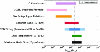
Figure 4. Ranges of disk masses resulting from the uncertainties in total masses derived from dust and gas and measured by various techniques. The dashed vertical line indicates our reference mass for this exercise, taken to be the mass estimate for a disk with 1.3 mm emission of 25 mJy around a 1 M⊙ star (the median value in Andrews et al. Reference Andrews, Rosenfeld, Kraus and Wilner2013). The coloured bars mark how the mass estimate may change depending on the method. Using a gas tracer, depending on: C abundance (purple; Kama et al. Reference Kama2016a), CO depletion/freeze out (pink, Thi et al. Reference Thi2001; Du et al. Reference Du, Bergin and Hogerheijde2015), isotopologue relations (yellow; Miotello et al. Reference Miotello, Bruderer and van Dishoeck2014), and changing the gas/dust ratio between 10–200 (red; Panić et al. Reference Panić, Hogerheijde, Wilner and Qi2009; Riviere-Marichalar et al. Reference Riviere-Marichalar2013). Using a dust indicator: with a complete SED lacking the mm data but including mid-IR (light blue) and far-IR (dark blue; Sicilia-Aguilar et al. Reference Sicilia-Aguilar2011; Sicilia-Aguilar et al. 2015a; Currie & Sicilia-Aguilar Reference Currie and Sicilia-Aguilar2011), varying the assumed dust temperature (green; Andrews et al. Reference Andrews, Rosenfeld, Kraus and Wilner2013), and changing the maximum grain size between 10 μm and 1 mm (black; Miyake & Nakagawa Reference Miyake and Nakagawa1993; Henning & Stognienko Reference Henning and Stognienko1996).
The possibility of high-sensitivity gas tracers with ALMA would be a key, both to obtain better mass estimates as well as to resolve the potential radial dependency of grain sizes and gas/dust ratios throughout the disk. A robust way to estimate gas masses would require simultaneous modeling of spatially resolved CO isotopologue data, together with sub-mm imaging, and also [O I] 63 μm and [C I] emission (Woitke et al. Reference Woitke2016; Kama et al. Reference Kama2016a, Reference Kama2016b). Building on these and other works, future ALMA observations together with a better understanding of the disk chemistry will be keys to determine the disk masses.
5 ACCRETION
In this section, we discuss the observables of mass accretion onto the star, and several outstanding problems raised by observations. Accretion plays a central role in disk dispersal: Angular momentum transport and energy minimisation in the disk, driven by viscosity, cause mass transport inwards and accretion onto the star, while it also produces expansion of the disk outer radius in time (Gammie Reference Gammie1996; Hartmann et al. Reference Hartmann, Calvet, Gullbring and D’Alessio1998, Reference Hartmann, D’Alessio, Calvet and Muzerolle2006). While viscous evolution alone would require disk evolutionary times much longer than observed (Hartmann et al. Reference Hartmann, Calvet, Gullbring and D’Alessio1998), accretion is a powerful mechanism: It connects the whole disk and the star, having the potential to affect the early stellar evolution (Baraffe, Chabrier, & Gallardo Reference Baraffe, Chabrier and Gallardo2009), the architecture of the nascent planetary system and the migration of planets (Lubow & Ida Reference Lubow and Ida2010), and the disk structure (such as the mass distribution in the inner disk and the dust vs. gas disk radius).
There are two main theories to explain how accretion proceeds onto the star: boundary layer (BL; the gas accretes directly from the disk to the central star) and MA (the gas from the inner disk channeled through the stellar magnetic field lines). Early works focussed on the BL scenario for both TTS and HAeBes (Bertout, Basri, & Bouvier Reference Bertout, Basri and Bouvier1988; Basri & Bertout Reference Basri and Bertout1989; Blondel & Djie Reference Blondel and Djie1994, Reference Blondel and Djie2006). Nevertheless, MA is since long widely accepted for TTS (Uchida & Shibata Reference Uchida and Shibata1985; Koenigl Reference Königl1991; Shu et al. Reference Shu1994; Alencar Reference Alencar2007), supported by evidence from near-UV excess, emission line profiles, observed magnetic (B-) fields, rotational modulation of line profiles, and the presence of outflows and jets. MA also seems to be drive accretion in brown dwafs (Riaz Reference Riaz2013) and has been temptatively proposed for accreting planets in formation (Lovelace, Covey, & Lloyd Reference Lovelace, Covey and Lloyd2011; Zhu Reference Zhu2015). Several lines of evidence suggest that accretion could also be magnetically driven in late type HAe stars, as suggested by spectro-polarimetry (Vink et al. Reference Vink, Drew, Harries and Oudmaijer2002; Mottram et al. Reference Mottram, Vink, Oudmaijer and Patel2007) and near-UV continuum excesses (Muzerolle et al. Reference Muzerolle, D’Alessio, Calvet and Hartmann2004; Donehew & Brittain Reference Donehew and Brittain2011; Mendigutía et al. Reference Mendigutía2011b, Reference Mendigutía2013; Fairlamb et al. Reference Fairlamb2015). Near-UV/optical/NIR spectral lines also show profiles similar to those of TTS (Mendigutía et al. Reference Mendigutía2011a; Cauley & Johns-Krull Reference Cauley and Johns-Krull2014, Reference Cauley and Johns-Krull2015), which can be reproduced from MA line modelling (e.g. UX Ori and BF Ori in Muzerolle et al. Reference Muzerolle, D’Alessio, Calvet and Hartmann2004 and Mendigutía et al. Reference Mendigutía2011b, respectively).
The small/non-detected B-fields in HAeBes is commonly argued against MA operating in these objects. Although their internal structure with radiative envelopes did not predict the presence of B-fields and related high-energy emission, X-rays are regularly detected towards HAeBe stars (especially, amongst those with M < 3M⊙, e.g. Feigelson et al. Reference Feigelson, Gaffney, III, Hillenbrand and Townsley2003; Preibisch et al. Reference Preibisch2005; Forbrich & Preibisch Reference Forbrich and Preibisch2007; Stelzer et al. Reference Stelzer, Robrade, Schmitt and Bouvier2009). The minimum B-field required to drive MA is strongly dependent on the stellar properties (Johns-Krull, Valenti, & Koresko Reference Johns-Krull, Valenti and Koresko1999), so if B-fields of ~ 1 kG are necessary in TTs, much smaller B-fields of only hundreds of G or less would be enough for the HAeBes (see the discussion in Mendigutía et al. Reference Mendigutía2015b; Fairlamb et al. Reference Fairlamb2015). There are clear indications that the accretion mechanism changes at some point within the HAeBe regime (e.g. Mottram et al. Reference Mottram, Vink, Oudmaijer and Patel2007; Mendigutía et al. Reference Mendigutía2011b; Fairlamb et al. Reference Fairlamb2015), and there are several early-type HBes for which MA is definitely not able to reproduce the strong near-UV excesses observed (Mendigutía et al. Reference Mendigutía2011b; Fairlamb et al. Reference Fairlamb2015). Understanding accretion in HBes would need a new approach, perhaps returning to BL (Cauley & Johns-Krull Reference Cauley and Johns-Krull2015) or considering similar mechanisms (but for accretion, not decretion) as in classical Bes (Patel, Sigut, & Landstreet Reference Patel, Sigut and Landstreet2015).
Observationally, accretion rates are ultimately derived from the accretion luminosity. The accretion luminosity can be estimated from the veiling, continuum excess (Gullbring et al. Reference Gullbring, Hartmann, Briceño and Calvet1998), or emission line luminosity (Natta et al. Reference Natta, Testi, Randich and Muzerolle2005; Fang et al. Reference Fang, van Boekel, Wang, Carmona, Sicilia-Aguilar and Henning2009; Alcalá et al. Reference Alcalá2014). To determine the luminosity due to accretion, the spectral type and extinction of the star must be well-constrained, especially if the accretion luminosity is small compared to the stellar luminosity. The lowest accretion rate that can be detected depends on how other processes, such as activity and winds, affect the accretion tracers (Sicilia-Aguilar, Henning, & Hartmann Reference Sicilia-Aguilar, Henning and Hartmann2010; Manara et al. Reference Manara2013). This makes the methods relying on direct accretion luminosity estimates (measuring the veiling, the Balmer jump, or U band excess) more powerful than those relying on line emission (as showed in Figure 5). When detailed information on the stellar properties (spectral type, luminosity, extinction, typical activity levels in similar but diskless stars) is available, the detection limits for accretion onto solar-type stars (late K-early M) can be as low as 10−11 M⊙ yr−1 (Sicilia-Aguilar et al. Reference Sicilia-Aguilar, Henning and Hartmann2010), while for very low-mass stars and BD, accretion rates as low as 10−13 M⊙ yr−1 can be inferred (Natta et al. Reference Natta, Testi, Neri, Schepherd and Wilner2004; Herczeg, Cruz, & Hillenbrand Reference Herczeg, Cruz and Hillenbrand2009). On the other hand, accretion-related spectral lines have the advantage of providing velocity information. Metallic lines observed in accreting stars (Hamann & Persson Reference Hamann and Persson1992) span a large range of critical densities and temperatures, thus tracing material in various physical conditions and different locations within the accretion-related structures. The velocities can be used to estimate the extent of accretion columns via Doppler tomography, using the strong Hα and Hβ lines (Muzerolle, Calvet, & Hartmann Reference Muzerolle, Calvet and Hartmann2001; Muzerolle et al. Reference Muzerolle, Hillenbrand, Calvet, Briceño and Hartmann2003; Lima et al. Reference Lima, Alencar, Calvet, Hartmann and Muzerolle2010; Alencar et al. Reference Alencar2012), or the many metallic emission and absorption lines (Beristain, Edwards, & Kwan Reference Beristain, Edwards and Kwan1998, Reference Beristain, Edwards and Kwan2001; Sicilia-Aguilar et al. Reference Sicilia-Aguilar2012; Petrov et al. Reference Petrov, Gahm, Herczeg, Stempels and Walter2014; Sicilia-Aguilar et al. Reference Sicilia-Aguilar2015b).
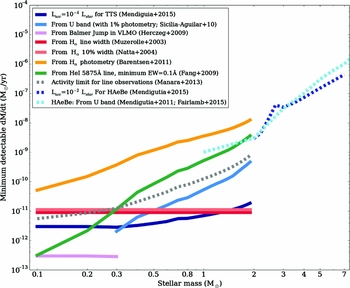
Figure 5. Lowest detectable accretion rates for stars with different masses, using different techniques. The (Siess, Dufour, & Forestini Reference Siess, Dufour and Forestini2000) isochrone track for 3 Myr-old stars is used to transform between mass and luminosity. A distance of 140 pc is assumed. See references in text for details on the various techniques.
5.1. Accretion as a probe of the disk and the star
Accretion involves the whole disk, as transport through the disk is needed to maintain the accretion rate over time. Therefore, the presence (or lack) of accretion is a powerful tool to investigate disk structure and physical processes. Although it is possible to measure accretion rates down to 10−11 M⊙ yr−1 for solar-type starsFootnote 7 , we find that only very few stars have such low rates, suggesting that accretion stops quickly after reaching levels below ~ 10−10 M⊙ yr−1 (Sicilia-Aguilar et al. Reference Sicilia-Aguilar, Henning and Hartmann2010). This is consistent with the predictions of photoevaporation as a process removing the inner gaseous disk in a relatively short time (Clarke et al. Reference Clarke, Gendrin and Sotomayor2001; Alexander, Clarke, & Pringle Reference Alexander, Clarke and Pringle2006; Gorti, Dullemond, & Hollenbach Reference Gorti, Dullemond and Hollenbach2009). For solar-type stars, stopping accretion seems very rare unless dramatic changes have occurred to the whole disk (such as strong mass depletion Sicilia-Aguilar et al. Reference Sicilia-Aguilar, Kim, Sobolev, Getman, Henning and Fang2013b, Reference Sicilia-Aguilar2015a). This is in agreement with accretion being a global process that connects the inner and the outer disk and can be used as an indicator of global disk evolution (Sicilia-Aguilar et al. Reference Sicilia-Aguilar2015a; Manara et al. Reference Manara2016).
The presence (or lack) of accretion in disks with inner holes (identified from SEDs) also clearly separates two classes amongst transition disks around TTS: accreting and non-accreting ones. While essentially all primordial or ‘full’ disks show signs of accretion (Sicilia-Aguilar et al. Reference Sicilia-Aguilar, Kim, Sobolev, Getman, Henning and Fang2013b), between 30–50% of transition disks show none (narrow emission lines, no UV excess, no veiling; Fang et al. Reference Fang, van Boekel, Wang, Carmona, Sicilia-Aguilar and Henning2009; Sicilia-Aguilar et al. Reference Sicilia-Aguilar, Henning, Juhász, Bouwman, Garmire and Garmire2008b, Reference Sicilia-Aguilar, Henning and Hartmann2010). Although less explored, differences in the accretion rate between primordial and transitional disks have also been observed for HAeBe stars (Mendigutía et al. Reference Mendigutía2012). Our understanding of the evolutionary stage of transition disks will improve with multi-wavelength data (see Section 7).
Accretion is also connected to the stellar properties, since the accreting matter is channelled onto the star by the stellar magnetic field (Koenigl Reference Königl1991). Therefore, studies of the properties and distribution of accretion columns can also help to study the magnetic field topology of the star, intimately related to the stellar structure and evolution (e.g. Donati et al. Reference Donati2011, Reference Donati2013; Gregory et al. Reference Gregory, Jardine, Cameron and Donati2006, Reference Gregory2014). Time-resolved Hα and metallic line emission spectroscopy are promising ways to study the presence, distribution, and evolution of accretion-related hot spots, which can be connected to the structure of the stellar magnetic field (Alencar et al. Reference Alencar2012; Sicilia-Aguilar et al. Reference Sicilia-Aguilar2015b). Extension of these studies to other stars have the power to provide new information on stellar properties during a key time in their evolution.
5.2. Open problems for accretion: disk masses and accretion tracers
An outstanding problem regarding the disk’s gas content is that accretion rates and observed disk masses are often in conflict: Considering the measured disk masses (dust- or gas-based) and the observed accretion rates, a significant fraction of stars are expected to fully drain their disks in timescales shorter (sometimes, by several orders of magnitude) than the usual disk lifetimes. The situation can be extreme for some strong accretors with not-so-massive disks (Hartmann et al. Reference Hartmann, D’Alessio, Calvet and Muzerolle2006; Sicilia-Aguilar et al. Reference Sicilia-Aguilar2008a; Sipos et al. Reference Sipos2009; Liu et al. Reference Liu2016; Kóspál et al. Reference Kóspál2016).
Figure 6 shows the extent of the problem: If we compare the observed disk masses (Andrews et al. Reference Andrews, Rosenfeld, Kraus and Wilner2013) with the mass ingested by the star during 2 Myr (which is shorter than the median disk lifetime of ~ 3 Myr; Sicilia-Aguilar et al. Reference Sicilia-Aguilar2006a), there is a clear divergence. This is a problem that affects both TTS (Andrews & Williams Reference Andrews and Williams2007; Sicilia-Aguilar et al. Reference Sicilia-Aguilar2011) and HAeBes (Mendigutía et al. Reference Mendigutía2012), although the difference is negligible for stellar masses M * < 0.2 M⊙ and increases with the mass of the star (see Figure 6). Assuming that stars have variable accretion and that they only spend a small part of their lives accreting at very high rates could help solving the problem, although there is no evidence of short-term strong accretion variability amongst most 1–10 Myr old stars (Sicilia-Aguilar et al. Reference Sicilia-Aguilar, Henning and Hartmann2010; Costigan et al. Reference Costigan2012, Reference Costigan, Vink, Scholz, Ray and Testi2014). Moreover, the problem still persits if the accretion rate is taken to be the median accretion rate observed for stars aged ~ 3–4 Myr (Sicilia-Aguilar et al. Reference Sicilia-Aguilar, Henning and Hartmann2010), scaling the results from solar-type stars to higher and lower masses following the usual Ṁ∝M 2 * relation (Natta et al. Reference Natta, Testi, Randich and Muzerolle2005). This points to an overestimation of the accretion rates (or the time stars spend accreting), or an underestimation of the disk masses, or both.
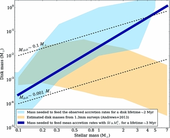
Figure 6. Disk masses as measured by observations, and as expected from the need to support the observed accretion rates during a lifetime of 2–3 Myr. The black dotted lines represent the usual limits of disk masses between 0.1–10% of the mass of the star. The yellow area displays the disk masses measured by (Andrews et al. Reference Andrews, Rosenfeld, Kraus and Wilner2013). The blue region represents the expected disk masses for the whole range of accretion rates observed, and a disk lifetime of 2 Myr (which is typically lower than the median disk lifetime of ~ 3 Myr). The dark blue line represents the expected disk masses considering the median accretion rate at 4 Myr and an accretion lifetime of 3 Myr (Sicilia-Aguilar et al. Reference Sicilia-Aguilar, Henning and Hartmann2010).
At present, the uncertainty in the accretion rates (especially if derived from UV or accretion luminosities for stars with well-known spectral types and extinctions) is smaller than the uncertainty in the total disk mass (or at least, in the part of gas mass that we can measure; see Figure 4). Freezing-out of gas tracers and the potential changes in the gas/dust ratio as the disk evolves are clear problems in the estimation of gas masses. We may be able to solve this mismatch as more detailed, spatially resolved gas observations become available. The problem could be solbed by assuming gas/dust ratio ~ 1 000, but current observations, including data from several Herschel Consortia, rather suggest that if any, the gas/dust ratios may be lower than in the ISM (e.g. Riviere-Marichalar et al. Reference Riviere-Marichalar2013).
Shorter disk and accretion lifetimes for HAeBe could contribute to solve the problem, and indeed accretion rates in HAeBe are expected to drop more abruptly than for TTS (Mendigutía et al. Reference Mendigutía2012). Changing the way the accreted matter reaches the star does not help: BL results in higher accretion rates than MA, making the problem worse. Considering that the correlations between the accretion rate and the disk mass expected from viscous accretion models (Hartmann et al. Reference Hartmann, Calvet, Gullbring and D’Alessio1998) often remain elusive, the mass/accretion disagreement may be a signature of our difficulties estimating total disk masses, where dust masses are by far better determined than gas masses—but they only trace a minimal part of the disk (Manara et al. Reference Manara2016).
Another open problem is whether all accretion tracers measure the same thing. The observed correlations between line and accretion luminosities do not necessarily indicate a physical relation between both (Mendigutía et al. Reference Mendigutía2015a). Spectro-interferometry of Hα, Brγ, and CO, with instruments on Keck-I, CHARA, and VLTI, shows that although the Hydrogen lines are often used as a proxy to estimate mass accretion rates, the bulk of the emission arises in regions more extended than expected from MA. Indeed, several observations reveal extended emission, consistent with the base of a disk wind (Kraus et al. Reference Kraus2008; Benisty et al. Reference Benisty2010c; Weigelt et al. Reference Weigelt2011; Garcia Lopez et al. Reference Lopez2015; Caratti o Garatti et al. Reference Caratti o Garatti2015). In the same objects, in particular, the most massive ones, the displacement of the photocentre is consistent with Keplerian motion (Ellerbroek et al. Reference Ellerbroek2014; Kraus et al. Reference Kraus2012; Mendigutía et al. Reference Mendigutía2015b), although it might be difficult to disentangle the emission from the disk from the emission from the base of the disk wind (Kurosawa et al. Reference Kurosawa2016).
Moreover, observed emission lines often suggest that accretion-related structures are not monolithic entities, but include gas with different physical conditions. Several stars (DR Tau, Petrov et al. Reference Petrov, Gahm, Stempels, Walter and Artemenko2011; S CrA, Gahm et al. Reference Gahm, Walter, Stempels, Petrov and Herczeg2008; EX Lupi, Sicilia-Aguilar et al. Reference Sicilia-Aguilar2012, Reference Sicilia-Aguilar2015b; RU Lupi, Dodin & Lamzin Reference Dodin and Lamzin2012, Reference Dipierro, Laibe, Price and Lodato2013) show evidence of line-dependent veiling or ‘veiling-by-lines.’ In these cases, part of the accretion luminosity is not emitted as continuum, but as spectral lines, filling in the stellar photospheric lines to different extents. The strength of the veiling on a given line depends on the physical conditions on the accretion structures (temperature, density) and the line formation conditions/atomic parameters of the given line. The properties and structure of the accretion column may vary, depending on their number and structure, resulting in strong line differences even in objects with similar accretion rates (Sicilia-Aguilar et al. Reference Sicilia-Aguilar2015b). Line-dependent veiling can dominate the spectrum during times of high accretion, resulting in strong, broad line emission (Kóspál et al. Reference Kóspál2008; Sicilia-Aguilar et al. Reference Sicilia-Aguilar2012; Holoien et al. Reference Holoien2014). Line veiling has been poorly explored for the general population, and could potentially affect the estimates of accretion rates, especially for objects with very low accretion or in cases where the accretion columns are optically thin. Nevertheless, line-dependent veiling can be also used as a tool to estimate the physical conditions in the accretion columns and accreting material (Sicilia-Aguilar et al. Reference Sicilia-Aguilar2012, Reference Sicilia-Aguilar2015b) (see Section 6), although extracting broad, faint lines from the stellar spectrum can be hard.
6 DISK INSIGHTS FROM VARIABLE PHENOMENA AND DISK DYNAMICS
In this section, we discuss the stellar variability and the dynamical effects observed in the disk as means to explore the time dimension in disks. Different parts of the star+disk system respond to different timescales (stellar rotation, keplerian rotation), and the physical processes involved in disk dispersal are also strongly dynamical.
6.1. Photometric and spectroscopic variability
Photometric and spectroscopic variability is a defining characteristic of pre-main sequence stars (PMS; Joy Reference Joy1945; Herbst et al. Reference Herbst, Herbst, Grossman and Weinstein1994; Briceño et al. Reference Briceño2001; Alencar, Johns-Krull, & Basri Reference Alencar, Johns-Krull and Basri2001). Photometric monitoring campaigns at optical wavelengths covering timescales of days to months reveal three main causes for the variations in low-mass TTS (Herbst et al. Reference Herbst, Herbst, Grossman and Weinstein1994): periodic, cold (chromospheric) spots on the stellar surface, non-periodic hot (accretion-related) spots, and more extreme dimmings (up to 3–4 mag in the optical on timescales of one week) accompanied by polarisation changes, caused by circumstellar material in the line of sight (UXOr-type variability; see e.g Grinin et al. Reference Grinin, Kiselev, Chernova, Minikulov and Voshchinnikov1991; Natta et al. Reference Natta, Grinin, Manings and Ungerechts1997; Rodgers Reference Rodgers2003). A sensitive photometric survey with CoRoT identified several common types of variability and was able to probe the presence of stable and unstable accretion, stellar hot spots, and common occultations by inner disk structures such as accretion columns and warps (McGinnis et al. Reference McGinnis2015). While hot and cold spots explain most of the variability observed in TTS, HAeBes, without cold spots, no chromospheres, and accretion shock temperatures comparable to their effective temperatures, are dominated by UXOr-type variability (Muzerolle et al. Reference Muzerolle, D’Alessio, Calvet and Hartmann2004; Mendigutía et al. Reference Mendigutía2011b, Reference Mendigutía2011a).
The Spitzer Space Telescope, especially during its warm mission, has been used to study infrared variability in a number of nearby clusters (Morales-Calderón et al. Reference Morales-Calderón2009; Poppenhaeger et al. Reference Poppenhaeger2015; Rebull et al. Reference Rebull2015; Morales-Calderón et al. Reference Morales-Calderón2011; Günther et al. Reference Günther2014; Wolk et al. Reference Wolk2015; Flaherty et al. Reference Flaherty2013; Cody et al. Reference Cody2014). These studies find that 60–90% of the young stellar objects are variable in the infrared, with variability being stronger and more common amongst Class I sources and weaker and less common amongst Class III sources, with typical fluctuations of a few tenths of a magnitude. While many of these studies are focussed on daily-to-weekly fluctuations, year-to-year fluctuations have been seen by both Spitzer (Rebull et al. Reference Rebull2014; Megeath et al. Reference Megeath2012) and ground-based NIR studies (Scholz Reference Scholz2012; Wolk, Rice, & Aspin Reference Wolk, Rice and Aspin2013; Parks et al. Reference Parks, Plavchan, White and Gee2014; Rice et al. Reference Rice, Reipurth, Wolk, Vaz and Cross2015). Full disks tend to show a flatter wavelength dependence of their variability over the 2–10 μm region (Megeath et al. Reference Megeath2012; Kóspál et al. Reference Kóspál2012), but some changes in colour have been seen. The 3–5 μm variability can be explained by a mix of extinction and disk variability (Poppenhaeger et al. Reference Poppenhaeger2015; Wolk et al. Reference Wolk2015), while ground-based NIR studies find similar results along with additional contributions from star spots (Carpenter, Hillenbrand, & Skrutskie Reference Carpenter, Hillenbrand and Skrutskie2001; Parks et al. Reference Parks, Plavchan, White and Gee2014), due to the larger fraction of stellar emission at shorter wavelengths.
Variability at different wavelengths (e.g. optical vs. IR) and spectroscopic variability (in emission and absorption lines, affecting the flux or the line profiles) can be very different for the same star. Campaigns to monitor variability at different wavelengths simultaneously provide information on the process that causes the variable events (e.g. extinction by disk material, compared to variations in the accretion rate/accretion luminosity; Eiroa et al. Reference Eiroa2000, Reference Eiroa2002; Morales-Calderón et al. Reference Morales-Calderón2009).
6.2. Stellar variability and variable accretion
Accretion variability is a highly debated topic, although part of the discussion depends on how one measures accretion: Using the UV-excess as tracer, the accretion rate variations over few-year timescales are small, typically less than 0.5 dex both in TTS (Sicilia-Aguilar et al. Reference Sicilia-Aguilar, Henning and Hartmann2010; Costigan et al. Reference Costigan2012; Venuti et al. Reference Venuti2015) and HAeBes (Mendigutía et al. Reference Mendigutía2011b, Reference Mendigutía2013). Line variability has been also used to study accretion variations, since accretion-related emission lines can change quite dramatically in flux and profile. However, these lines are affected by other physical processes, so even though the variations in line intensity and profile are stronger in stars with variable accretion (Alencar et al. Reference Alencar, Johns-Krull and Basri2001; Herbig Reference Herbig2008; Sicilia-Aguilar et al. Reference Sicilia-Aguilar2012), rotational modulation of the line intensities, and/or profiles is also observed in stars with relatively constant accretion (Alencar et al. Reference Alencar2012; Costigan et al. Reference Costigan, Vink, Scholz, Ray and Testi2014; Sicilia-Aguilar et al. Reference Sicilia-Aguilar2012, Reference Sicilia-Aguilar2015b). This effect has led to proposing stable and unstable accretion regimes, depending on whether accretion proceeds via well-defined channels (stable) vs. multiple, quickly changing fingers (unstable; Kurosawa & Romanova Reference Kurosawa and Romanova2013; Takami et al. Reference Takami2016).
Without detailed time-resolved data, it is often hard to determine whether accretion itself is variable, or whether there are rotational modulations due to an irregular distribution of accretion columns over the stellar surface (Alencar et al. Reference Alencar2012; Costigan et al. Reference Costigan2012, Reference Costigan, Vink, Scholz, Ray and Testi2014). Nevertheless, some objects (FUOr and EXOr) display dramatic accretion variations, with increases in the accretion rate up to a few orders of magnitude. Both classes were initially identified from optical variability, and their nature, evolutionary stage, and the link between them and the rest of PMS stars remains open to debate (e.g. review in Audard et al. Reference Audard, Beuther, Klessen, Dullemond and Henning2014, amongst others).
Besides their interest as part of the star-formation pathway and disk evolution, stars with variable accretion are key target to understand the physics of disks, by observing how the disk reacts to a sudden increase in the accretion rate. The luminosity variations associated to increased accretion episodes can dramatically affect the disk properties, processing the amorphous dust in the disk, and creating crystalline silicates (Ábrahám et al. Reference Ábrahám2009), and changing the gas composition in the planet-formation region by evaporating icy bodies and destroying organic molecules (Banzatti et al. Reference Banzatti2012). An increased disk heating can also shift the water snow line to much larger disk radii during an accretion outburst, as discovered in the FUor disk of V883 Ori (Cieza et al. Reference Cieza2016), producing ice evaporation and dust fragmentation over a disk region where planets would otherwise typically form (Banzatti et al. Reference Banzatti2015b). Subsequent evolution of the disk after outbursts reveals longer term processes happening in inner and out disk regions, such as the draining of inner disk gas by the central star (Banzatti et al. Reference Banzatti, Pontoppidan, Bruderer, Muzerolle and Meyer2015a; Goto et al. Reference Goto2011) and the redistribution of crystalline silicates to larger radial distances by disk winds (Juhász et al. Reference Juhász2012), allowing us to explore disk parameters that are otherwise hardly observable (disk mass budgets, disk viscosity, radial transport).
6.3. Time-resolved data as a means to trace disk and stellar properties
Time-resolved data allows to probe phenomena that involve variability, but they also allow us to access processes with well-defined timescales, such as stellar rotation, rotational modulation of accretion, companion orbits, and disk rotation. It is specially powerful to track relatively short timescales (hours–days), which typically correspond to spatial scales that are beyond the current direct resolution limits (e.g. stellar spots, accretion columns at few stellar radii, structures, and clumps on the inner disk rim at sub-AU scales).
The puffed-up inner rim may cause a radial part of the inner disk to be in shadow (Natta et al. Reference Natta2001; Dullemond et al. Reference Dullemond, Dominik and Natta2001; Dullemond & Dominik Reference Dullemond and Dominik2004; Isella & Natta Reference Isella and Natta2005). Although shadowing by features in the inner disk rim is more common amongst intermediate-mass stars, evidence for occultations by clumpy inner disks has been found for objects down to the BD regime (Scholz, Mužić, & Geers Reference Scholz, Mužić and Geers2015). One common subgroup are the ‘dippers’ or ‘AA-Tau’-like objects. The prototype is AA-Tau, which exhibits periodic extinction events that have been traced back to a warp at the interface of the disk and stellar magnetic field that periodically obscures they star as it rotates (e.g. Bouvier et al. Reference Bouvier2003). While this behavior is seen more often in the optical (where the extinction is stronger), it provides insight on the inner disk since it is the disk that is doing the obscuring. AA-Tau events occur in ~ 30% of the young stellar objects (Alencar et al. Reference Alencar2010; Cody et al. Reference Cody2014), with rapid extinction events associated with obscuration by material in the accretion flow (Stauffer et al. Reference Stauffer2014) and longer, quasi-periodic events associated with warps in the disk (McGinnis et al. Reference McGinnis2015).
Quasi-periodic dippers can be used to determine the height of the inner wall, which can vary by ~ 10% from one period to the next (McGinnis et al. Reference McGinnis2015). This is similar to the ‘seesaw’ behaviour seen in pre-transition disks, in which the short-wavelength flux increases (decreases) as the long-wavelength flux decreases (increases) (Muzerolle et al. Reference Muzerolle2009; Espaillat et al. Reference Espaillat2011; Flaherty et al. Reference Flaherty2011, Reference Flaherty2012), which has been successfully modelled by a variable inner disk height.
Azimuthally narrow shadowing structures at < 1AU in the optically thick inner disk height affect the illumination of part or all of the outer disk. They have orbital timescales comparable to the light travel time to the outer edge of the disk. As a result, the shadows cast by any such structures will be curved, and can take a range of shapes from nearly linear to strongly curved spirals (Kama, Pinilla, & Heays Reference Kama, Pinilla and Heays2016c). Fitting the shape of such features, we can constrain the orbital properties of spatially unresolved structures in the inner disk, as well as provide an independent constraint on the vertical structure and absolute radial size of the disk. The 1mag variability of the HD 163296 disk in scattered light imaging spanning 6 yrs may be direct evidence for time-variable shadowing (Sitko et al. Reference Sitko2008; Wisniewski et al. Reference Wisniewski2008). The systematic study of such variations could constrain the presence and properties of large-mass substellar companions and various instabilities (Sitko et al. Reference Sitko2008).
Polarisation, despite being a main technique to study the extended disk (see Section 3.2), can be also used to study variability of PMS and the innermost disk through unresolved photo-polarimetry. Unpolarised stellar light that scatters off dust grains in a circumstellar environment will become linearly polarised. The photometric signal from star and disk combined will be partially polarised when the emission from the stellar photosphere deviates from spherical symmetry (e.g. stellar spots), when part of the stellar surface is obscured by the disk (e.g. flaring inner disk), or the circumstellar disk is inclined or non-axisymmetric, producing polarisation levels of 0–2% (e.g Oudmaijer et al. Reference Oudmaijer2001). Photo-polarimetric variability can thus reveal changes in the stellar photosphere and the inner disk, for example, by a warped inner disk which is coupled to the stellar magnetic field leading to variable obscuration of the star (e.g. Manset et al. Reference Manset2009).
Time-resolved spectroscopy is a further tool to study the complexity of parts of the star-disk system that are beyond the possibilities of direct resolution. Applied to absorption lines, it can be used to track the orbits of atomic gas packages in the disk and to study atomic gas dynamics (Mora et al. Reference Mora2002, Reference Mora2004). Bright emission lines like Hα and Hβ can be used to study the stability of accretion (Alencar et al. Reference Alencar2012; Kurosawa & Romanova Reference Kurosawa and Romanova2013). Metallic emission lines (Fe I, Fe II, Ti II, Mg I, Ca II, etc.; Hamann & Persson Reference Hamann and Persson1992) are specially valuable, since they are simpler than Hydrogen and Helium emission lines and span a large range of critical densities and temperatures, which allows to probe different regions within the accretion structures. Time-resolved spectroscopy of the metallic emission lines thus provides a ‘tomographic’ 3D view of accretion, tracing the location, extent, and physical properties of the accretion columns and associated hot spots (Sicilia-Aguilar et al. Reference Sicilia-Aguilar2012, Reference Sicilia-Aguilar2015b).
Time-resolved radial velocity data is also a classical means to determine the presence of planetary and binary companions. Nevertheless, the signatures of companions in young stars can be mimicked/masked by the presence of periodic signatures associated to stable accretion columns or stellar spots (Kóspál et al. Reference Kóspál2014; Sicilia-Aguilar et al. Reference Sicilia-Aguilar2015b). This makes it hard, but not impossible (if the star properties are well-constrained), to detect young planets (Johns-Krull et al. Reference Johns-Krull2016; Donati et al. Reference Donati2016; David et al. Reference David2016). Companions embedded in the disk are a potential tool to study disk properties. Accretion rate variations are normally random, but the presence of close-in stellar companions embedded in the disk can cause pulsed accretion (in L54361; Muzerolle et al. Reference Muzerolle, Furlan, Flaherty, Balog and Gutermuth2013) and periodic perturbations to the accretion-related wind (in GW Ori; Fang et al. Reference Fang2014). A companion in the disk acts as a ‘disk scanner’: It moves through a well-defined orbit that crosses (and potentially perturbs) the material in the inner disk. This allows us to use its disturbances to estimate the location of the launching point of the disk wind and where the bulk of the matter flow runs through the inner disk.
6.4. Disk dynamics
Radio interferometers not only can trace the spatial distribution of gas within a disk, but also its kinematic profile. To zeroth order, the gas in a disk is moving in Keplerian orbits around the central star(s). With small corrections due to the pressure gradient and the height of gas above the midplane (Rosenfeld et al. Reference Rosenfeld, Andrews, Hughes, Wilner and Qi2013), this motion can be used to ‘weigh’ the central star(s), as has been done in the AK Sco (Czekala et al. Reference Czekala2015) and DQ Tau (Czekala et al. Reference Czekala2016) binary systems.
Beyond Keplerian rotation, turbulence plays a large role in e.g. setting the relative velocity of small dust grains (Testi et al. 2014), regulating the accretion flow through the disk (Turner et al. Reference Turner2014), setting the vertical chemical structure (e.g. Owen et al. 2014), setting the minimum mass of gap opening planets (e.g. Kley & Nelson Reference Kley and Nelson2012), amongst many other effects. In part because of its importance, turbulence has received a great deal of attention in theoretical studies (see recent reviews by Armitage Reference Armitage2011; Turner et al. Reference Turner2014). The predominant theory for turbulence, magneto-rotational instability (MRI) predicts motions of a few tenths of the local sound speed in the upper few pressure scale heights of the outer disk (Miller & Stone Reference Miller and Stone2000; Flock et al. Reference Flock, Dzyurkevich, Klahr, Turner and Henning2011; Simon et al. Reference Simon, Hughes, Flaherty, Bai and Armitage2015), which translates to tens to hundreds of metres per second in the outer disk.
Given the weakness of this effect and its degeneracy with thermal broadening, observations have been less common than theoretical studies. The high spatial and spectral resolution of radio interferometers can overcome many of these complications, making them a promising source of observational constraints. Simon et al. (Reference Simon, Hughes, Flaherty, Bai and Armitage2015) demonstrated, using simulated ALMA CO observations of their shearing-box MRI simulations, that turbulence can change the peak-to-trough ratio of the CO spectrum, as well as the broadening in the images, removing some of the degeneracy with thermal broadening. Guilloteau et al. (Reference Guilloteau, Dutrey, Wakelam, Hersant, Semenov, Chapillon, Henning and Piétu2012) used CS, whose relatively high mass reduces the contribution from thermal broadening, to measure turbulence of ~ 0.5 c s in DM Tau. Flaherty et al. (Reference Flaherty2015) examined ALMA observations of HD 163296 and put an upper limit of only 0.03 c s on the turbulence in the outer disk, well below theoretical predictions. Hughes et al. (Reference Hughes, Wilner, Andrews, Qi and Hogerheijde2011) used high spectral resolution SMA observations of CO to derive an upper limit ( < 40 m s−1) in the TW Hya disk. Teague et al. (Reference Teague2016) examined ALMA data of TW Hya and tentatively detect turbulence at ~ 50–130 m s−1, while emphasising that uncertainties in the absolute calibration are a substantial limiting factor in these types of observations.
Other non-Keplerian effects have also been examined in recent years, often in response to new ALMA observations. Rosenfeld, Chiang, & Andrews (Reference Rosenfeld, Chiang and Andrews2014) modelled the rapid radial inflow of gas that can arise in transition disk systems with heavily depleted inner gaps. Casassus et al. (Reference Casassus2015) considered a warped disk in which the inner disk is tilted with respect to the outer disk. Dong et al. (Reference Dong, Vorobyov, Pavlyuchenkov, Chiang and Liu2016) estimates that signatures of gravitational instability should be detectable by ALMA in the gas dynamics of disks up to 400 pc distance. All these situations generate velocity differences on the order of the Keplerian velocity, which can be easily resolved over much of the disk. Salyk et al. (Reference Salyk2014) find evidence for molecular winds in CO observations of the binary AS 205 based on the kinematics of the extended emission. Shocks associated with spiral arms can create velocity jumps that are multiples of the local sound speed (Zhu et al. Reference Zhu, Dong, Stone and Rafikov2015) and surface density differences across the spiral arms that are potentially observable (Dipierro et al. Reference Dipierro, Lodato, Testi and Monsalvo2014; Hall et al. Reference Hall, Forgan, Rice, Harries, Klaassen and Biller2015).
The dynamical timescale of the outer disk stretches from decades to thousands of years, while the surface layers can respond rapidly to changes in illumination (Chiang & Goldreich Reference Chiang and Goldreich1997). This time dependence means that synoptic observations over many years can trace changes in structure as well as the response of the upper disk layers to variable illumination. HH 30, a nearly edge-on disk, exhibits variable reflection from the dust surface layers that can be explained by a central beam of light sweeping through the outer disk (Stapelfeldt et al. Reference Stapelfeldt1999). Accretion bursts can modify the solid-state features in disks, producing crystalline silicates and cometary material (Ábrahám et al. Reference Ábrahám2009). These newly created crystals can be used as a ‘contrast’ to track the mass flow within the disk: Follow-up of these crystals over months/years can be used to trace transport, mixing, turbulence, and viscosity through the disk (Juhász et al. Reference Juhász2012), even though disentangling the various transport mechanisms (wind, viscous transport, mixing on the vertical direction, turbulence) is not easy.
As the optical and IR (and soon also longer wavelengths) temporal baseline of observations in public databases grow, a new door to exploring long-period variability opens, including studing accretion variability on half a century term, spectral type changes associated to activity cycles, and constraining the long-timescale variations in protostars and FUor objects.
7 DISCUSSION: POWER AND LIMITATIONS OF MULTI-WAVELENGTH OBSERVATIONS
In this section, we discuss what we can learn from combining different observational techniques. We highlight their complementarity in terms of disk properties, outline the limitations of individual techniques, and discuss how the synergy of different observations can help to clarify outstanding problems in our understading of disk structure and evolution.
7.1. Understanding the degeneracies
Many of the uncertainties in our knowledge of disks result from incomplete observations, which lead to degeneracies when interpreting observations e.g. in terms of disk structure, gas/dust ratio, and dust properties. When interpreting dust continuum observations such as the SED or the IR visibilities and closure phases, there is a great degree of freedom in the selection of the dust shape, structure, composition (in particular, for featureless species such as carbon), and dust size distribution used to model the data. In addition, gas/dust ratios are usually unknown. Consequently, models are intrinsically degenerated: A large number of models may describe the data equally well. An additional complication comes from the parameter space being strongly non-continuous, so very different geometries, dust properties, and structures may provide a similarly good fit.
The stellar properties have a large impact on the disk structure as well as on its observables. The strong UV and X-ray irradiation by the young central star creates complicated and quite unique non-LTE conditions that cannot be studied elsewhere, which is one of the difficulties in understanding disk chemistry. In addition, a good characterisation of the star (spectral type, extinction, luminosity, activity) is the only way to observationally constrain many disk properties, such as ages and accretion rates (Sicilia-Aguilar et al. Reference Sicilia-Aguilar2006b, Reference Sicilia-Aguilar, Henning and Hartmann2010; Manara et al. Reference Manara2012, Reference Manara2013; Da Rio et al. Reference Da Rio, Jeffries, Manara and Robberto2014). The observational impact is larger for the parts of the disk SED for which the star provides a strong contribution, such as the NIR and the UV. The intrinsic variability of young stars is another potential source of inconsistency between non-simultaneous datasets.
Moreover, since disk emission is essentially stellar light reprocessed by the disk material, the central star plays an important role on observations, including the sensitivity (disks around late-type stars are significantly fainter at short wavelengths than their HAeBe counterparts, even if the disk masses are similar), contrast (e.g. detecting UV excesses and line emission from accretion in intermediate-mass stars is harder due to the higher continuum and deeper photospheric lines), and technical feasibility (e.g. NIR interferometry and scattered light observations require a certain magnitude for the central star). This produces observational biases with respect to the kind of disks we observe for stars with different masses, regarding for instance the detectability of holes and gaps, which need to be taken into account before deriving general properties and timescales.
The dust grain properties are a source of uncertainty and degeneracy for both unresolved and resolved observations. Usually, dust grains are assumed to have a distribution of sizes between a maximum and a minimum size, with a power-law exponent with slope − 3.5 (from collisional equillibrium). This relation can nevertheless change in protoplanetary disks: Grain sticking and fragmentation, together with the special physical conditions (very different from the ISM), can affect the grain properties and emissivity (Brauer, Dullemond, & Henning Reference Brauer, Dullemond and Henning2008; Zsom et al. Reference Zsom, Ormel, Dullemond and Henning2011). Dust size distributions can furthermore vary radially in the disk and with respect to the midplane due to size-dependent filtering by planets/companions and settling. The degeneracy on the dust properties can be reduced by modelling additional data sets. For example, a 10 μm spectrum covering the silicate emission can constrain the dust composition and size distribution in the upper layers of the disk. Scattered light images can constrain the amount of dust settling (e.g. Pinte et al. Reference Pinte, Ménard, Berger, Benisty and Malbet2008, Reference Pinte2009; Pinte et al. Reference Pinte2016), and sub-mm images constrain the mass of dust in large grains in spatial scales similar to the beam size, as well as the grain size and disk mass.
Understanding the gap physics from observations of individual disks with known planets could be also the starting point to interpret the observations of gaps and holes in other disks where the presence of planets is not known. Sparse aperture masking can be used for the detection and imaging of young planets and circumplanetary disks, and for the detection of complex structures within the disks (Biller et al. Reference Biller2014). ADI has also been used to search for protoplanets (Quanz et al. Reference Quanz2013). When accretion-related lines like Hα are observed with ADI, we can also detect accretion onto the protoplanets and study the structure of the gas within the cavity (Sallum et al. Reference Sallum2015). Spectro-astrometry of CO lines can be also applied to the search for planets and associated disks (Brittain et al. Reference Brittain, Najita and Carr2015; but see caveats in Fedele et al. Reference Fedele, Bruderer, van den Ancker and Pascucci2015). Spectro-astrometric signatures of accreting protoplanets should be detectable in optical and NIR emission lines (Hα, Brγ). NIR data, where the contrast with the star is lower, is very promising, athough X-shooter observations have not been successful so far (Whelan et al. Reference Whelan2015). Similarly, detailed studies of accretion and activity can help to improve our knowledge of these processes, helping to distinguish their effects on radial-velocities and photometry from those of planetary companions (Sicilia-Aguilar et al. Reference Sicilia-Aguilar2015b).
We still need to be careful with the difference between what has been determined about disks, and what relies on inferences. Some uncertainties can be addressed by an improvement in observational capability or in models. For example, with very high spatial resolution, we can determine a scale height directly by observing an edge-on disk in a tracer of choice. Or, if we need to know if a molecule varies greatly in abundance within a disk, we can apply a suitably large chemical network. However, other problems remain where we need to make sure that our inferences do not become established ‘facts’. Examples include the masses of disks and the signatures of planets, where our actual knowledge is much less sophisticated than, for example, the directly measurable properties of stars and exoplanets.
7.2. The power and limitations of unresolved, multi-wavelength data
One classical example of analysis of observations that is affected by multiple degeneracies is SED modelling and interpretation. The first problem is the lack of information on the gas, beyond what can be indirectly deduced from indicators such as accretion or disk flaring. Even though a good characterisation of the star and a relatively complete multi-wavelength dataset can exclude many possible disk structures, well-fitting detailed SED models for individual objects are often later contradicted by spatially resolved observations.
The broadband continuum SED of a disk can constrain the total dust mass up to particle sizes comparable to the longest observed wavelength, as well as the degenerate combination of gas disk flaring and large-grain settling. Although determining the size of an unresolved hole in the inner disk is strongly dependent on the assumed dust properties (including grain size) and shape of the inner rim (Calvet et al. Reference Calvet, D’Alessio, Hartmann, Wilner, Walsh and Sitko2002; Ratzka et al. Reference Ratzka2007; Sipos et al. Reference Sipos2009; Sicilia-Aguilar et al. Reference Sicilia-Aguilar2011), a complete optical and NIR SED can prove that a radial variation on disk properties (mass, grain sizes, and/or vertical scale heights) is needed to explain low IR fluxes (Furlan et al. Reference Furlan2005; D’Alessio et al. Reference D’Alessio, Calvet, Hartmann, Franco-Hernández and Servín2006; Sicilia-Aguilar et al. Reference Sicilia-Aguilar2013a). Similarly, even though the disk mass and scale height are highly degenerated if no millimetre data is available, there is a strong correlation between MIR data and millimetre observations (Lommen et al. Reference Lommen2010; Currie & Sicilia-Aguilar Reference Currie and Sicilia-Aguilar2011).
Far-IR data can provide strong constraints to the disk structure, specially important in case of faint and evolved disks (Sicilia-Aguilar et al. Reference Sicilia-Aguilar2015a). The shape of the MIR SED depends on both the disk flaring angle and the presence of cavities. MIR colours are in good correlation with the amount of detected scattered light, suggesting that both depend on the disk scale height. However, it is not known how often these disks may have non-detected gaps, since most (all?) of the resolved disks have gaps (Section 3).
SED interpretation relies on disk models, which can be applied to dust and gas observations. Codes such as, but not limited to, RADMC (Dullemond & Dominik Reference Dullemond and Dominik2004), DALIFootnote 8 (Bruderer et al. Reference Bruderer, van Dishoeck, Doty and Herczeg2012; Bruderer Reference Bruderer2013a), PRoDiMoFootnote 9 (Woitke, Kamp, & Thi Reference Woitke, Kamp and Thi2009), MCFOST (Pinte et al. Reference Pinte, Ménard, Duchêne and Bastien2006), and MCMax (Min et al. Reference Min, Dullemond, Dominik, de Koter and Hovenier2009) allow to model disks and to reconstruct observables (SEDs, resolved images) that can be directly compared to the data. Some models can simultaneously fit the SED, spatially resolved data, and atomic and molecular line fluxes. Published grids of models give guidance on how to combine the SED, line fluxes and profiles, and spatially resolved data to constrain various structure parameters, gas masses, snowline locations, and elemental abundances in the inner and outer disk (Gorti & Hollenbach Reference Gorti and Hollenbach2004; Robitaille et al. Reference Robitaille, Whitney, Indebetouw, Wood and Denzmore2006; Woitke et al. Reference Woitke2010; Kamp et al. Reference Kamp2011; Qi et al. Reference Qi2011; Woitke et al. Reference Woitke2016; Kama et al. Reference Kama2016a). A number of studies have fitted multi-wavelength data to determine the disk structure, gas mass, and C and O abundances (Gorti et al. Reference Gorti, Hollenbach, Najita and Pascucci2011; Tilling et al. Reference Tilling2012; Carmona et al. Reference Carmona2014; Du et al. Reference Du, Bergin and Hogerheijde2015; Kama et al. Reference Kama2016b). Care has to be taken when fitting disks with a pre-existing model grid, as this will not be able to pick up structures or disk properties that had not been previously included in the grid. Statistically similarly ‘good’ fits may miss key features (e.g., the silicate feature in the SED example in Figure 7), so ruling out disk structures incompatible with the observations is often a more powerful way to extract information from multi-wavelength SEDs than finding a good (but not unique) match (Sicilia-Aguilar et al. Reference Sicilia-Aguilar2011, Reference Sicilia-Aguilar2015a).
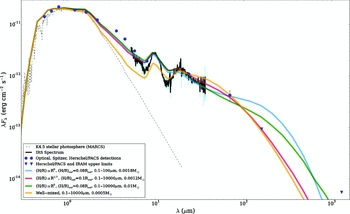
Figure 7. An example of how a very different (and non-continuous) distribution of disk models, including changes in disk mass, vertical structure, grain sizes, and settling) can provide similarly good fits to partial multi-wavelength data (based on Sicilia-Aguilar et al. Reference Sicilia-Aguilar2015a). The more data we include, the more models we can rule out. For the present example, NIR data can exclude a well-mixed gas and dust disk model, while the far-IR data and mm-wavelength upper limits put a strong constraint to the dust content in the disk. The fact that the silicate feature is not well-reproduced by any radially continuous disk model further indicates the presence of unresolved holes or gaps, which were not included in the model.
In summary, combined with statistically significant observations of many stars, SED modelling and interpretation is one of the most time-inexpensive methods to characterise the general properties and evolution of disks, especially faint ones around solar-type and low-mass objects. When large samples are included, the average global properties and timescales deduced provide a representation of the general behaviour. Even if the interpretation of individual objects may remain ambiguous, a fine-detail model is not always the answer: For instance, if we want to obtain a global view of the role of planets in disk dispersal, it may be enough to know what percentage of disks have gaps or holes consistent with planet formation, even if we do not know the precise sizes and locations of all the gaps and planets.
7.3. Planets and asymmetries: Intrinsic structure or evolution?
While there is a general consensus that the typical lifetime of disks is a few Myr, the way disk disperse and evolve and the observational signatures of disk dispersal processes are still uncertain. Recent observations show that it may be very hard to draw a clear line between disk structure and disk evolution. Disk gaps and holes are ubiquitously found by the increasing number of spatially or spectrally resolved observations, so that ‘classical’, primordial, continuous disks may indeed be the exception. This is especially true for HAeBe stars, for which both continuum and scattered light images show that almost all disks are asymmetric (Sections 2 and 3), but the (few) available high-resolution data on low-mass stars reveal potential evolutionary signatures, rings, and gaps, as well (e.g. HL Tau, TW Hya).
Radial asymmetries may form earlier than previously thought in the disk lifetime, even if most unresolved observations such as broadband SEDs are compatible with radially continuous disks. In this case, the ‘transitional’ phase of disks would be harder to define, as most disks would have holes/gaps/asymmetries from early on. The rate of structural changes in disks is essentially unknown, except in some extreme and rapidly variable cases (e.g. the triple system GW Ori, whose inner hole has suffered several dramatic changes in the last ~ 40 yrs; Fang et al. Reference Fang2014). The high frequency of gaps and holes observed would thus indicate that they are either produced all the time, or that they can survive for a few Myr.
Detailed, spatially resolved data and multi-wavelength observations of large samples of young disks around stars with different masses, will be a key to investigate which gaps and holes imply evolution (and which objects are the best candidates to be ‘about-to-disperse’ or ‘in transition’), and which may result from long-lasting processes operating through most of the disk lifetime. A comprehensive picture is still lacking but an effort to understand whether disks with(out) cavities, spirals, or rings, extended vs. compact structures, are different evolutionary stages or evolutionary paths starts to be possible (e.g. Maaskant et al. Reference Maaskant2013; Sicilia-Aguilar et al. Reference Sicilia-Aguilar, Kim, Sobolev, Getman, Henning and Fang2013b). Surveys that include disks around low-mass stars and around intermediate-mass stars will help to distinguish differences and similarities in their evolutionary paths (Banzatti & Pontoppidan Reference Banzatti and Pontoppidan2015). Being able to detect and resolve evolved disks around low-mass stars will also help to check whether gaps in disks around low-mass and intermediate-mass stars are similar entities, created by the same physical processes.
The morphology (and possibly also the nature) of the asymmetries observed in continuum and scattered light are different. The different coupling of small and large grains with the gas (which includes the possibility that large grains are not coupled at all; Laibe & Price Reference Laibe and Price2012a, Reference Laibe and Price2012b; Dipierro et al. Reference Dipierro, Laibe, Price and Lodato2016) is the likely cause, and can be used to explore the causes behind the asymmetries. Searching for counterparts of the scattered-light spirals and asymmetries at mm wavelengths can reveal whether these structures are ripples in the height distribution of micron size grains, or if they affect the whole disk, including larger grains (Akiyama et al. Reference Akiyama2016). Asymmetries affecting all disk components (gas, dust with different sizes) could be a signpost of processes such as gravitational instability (Durisen et al. Reference Durisen, Reipurth, Jewitt and Keil2007), which involves the entire disk structure.
Pinilla et al. (Reference Pinilla, Benisty and Birnstiel2012) and de Juan Ovelar et al. (2013) showed how the discrepancy between the location of the disk inner edge for micron- and mm-sized grains can be ascribed to the dust differentiation from the interaction with planets. The first observational proofs were obtained by Garufi et al. (Reference Garufi2013), later confirmed by others. Dong et al. (Reference Dong2012) showed that in some cases, a hole/gap for micron size grains may not even exist at all where seen for mm grains. Thus, a clear link between observed brightness decrease and intrinsic disk mass depletion has not yet been established, at least in scattered light.
Many authors have studied the effects of planet-disk interaction in the context of spirals (e.g. Juhász et al. Reference Juhász2015; Pohl et al. Reference Pohl2015; Dong et al. Reference Dong, Zhu and Whitney2015; Zhu Reference Zhu2015), although often the models do not provide fits with plausible physical conditions and/or perturber mass. No planets have been detected in spiral disks yet. More in general, there is no disk feature that could unanimously be ascribed to the interaction with known planets, even though the effects of known companions in disks holes and gaps has been documented for a few objects (Biller et al. Reference Biller2012; Fang et al. Reference Fang2014). Moreover, most of the transition disks studied in scattered light may be outliers in the nominal evolution of disks (and we are thus biased); otherwise, it is hard to reconcile the observed planetary system architectures with the disk observations (e.g. Dong et al. Reference Dong, Vorobyov, Pavlyuchenkov, Chiang and Liu2016). Finally, the aspect ratio and the location of the disk inner edge and its brightness profile can reveal information on the cavity nature, using scattered light (Quanz et al. Reference Quanz2013; Garufi et al. Reference Garufi2014; Avenhaus et al. Reference Avenhaus2014b) or MIR interferometry (Mulders et al. Reference Mulders2013).
In addition, there is a wide range in planetary mass and size that we cannot directly detect. The largest radio-detectable dust grains are centimetres across, while an accreting proto-planet will have a Hill sphere on AU scales. The only detectable sign of intermediate-mass planetesimals is perhaps in ‘falling evaporating bodies’, i.e. exo-comets that leave a redshifted spectroscopic signature towards the host star. In late-stage ‘debris’ disks, planetesimals should be present to regenerate dust that is short-lived compared to the host star; however, backtracking to the planetesimal sizes and locations is difficult. Further, some key physics on e.g. gas viscosity, turbulence motion, and ice formation is unclear, so that infering planet presence from apparently cleared gaps and cavities in disks is risky. In the future, observing forming planets—perhaps with JWST infrared imaging—or being able to apply usual planet detection techniques to young stars (which requires a very good understanding of the effects of accretion and activity on the planet tracers) may allow us to determine what actually makes a disk ‘proto-planetary’.
7.4. Disk mass and disk evolution
Although timescales favour the dispersal of protoplanetary disks from the inside-out (Hayashi et al. Reference Hayashi, Nakazawa, Nakagawa, Black and Matthews1985; Strom et al. Reference Strom, Strom, Edwards, Cabrit and Skrutskie1989), some disk dispersal processes such as gravitational instability may be more efficient in the outer, colder parts of the disk (Boss Reference Boss1997; Rice et al. Reference Rice, Armitage, Wood and Lodato2006). Moreover, observations of globally mass-depleted disks (with low small-dust content; Currie et al. Reference Currie, Lada, Plavchan, Robitaille, Irwin and Kenyon2009), extensive grain growth (Rodmann et al. Reference Rodmann, Henning, Chandler, Mundy and Wilner2006; Ricci et al. Reference Ricci2010), significantly settled disks (Furlan et al. Reference Furlan2005; D’Alessio et al. Reference D’Alessio, Calvet, Hartmann, Franco-Hernández and Servín2006; Sicilia-Aguilar et al. Reference Sicilia-Aguilar2011), and gaps at large distances (Brogan et al. 2015) suggest that a large degree of evolution may have happened through the whole disk before it starts to dissipate from the inside-out. A variety of evolutionary paths could also be behind the diversity of exoplanetary systems. From statistical studies using multi-wavelength, unresolved data, TTS appear to follow several distinct evolutionary paths. Transition disks with inner holes appear in two flavors: accreting and non-accreting (Fang et al. Reference Fang, van Boekel, Wang, Carmona, Sicilia-Aguilar and Henning2009; Sicilia-Aguilar et al. Reference Sicilia-Aguilar, Henning and Hartmann2010). Besides the presence/lack of accretion, the two classes also differ in the small-dust content of the disk (Sicilia-Aguilar et al. Reference Sicilia-Aguilar, Kim, Sobolev, Getman, Henning and Fang2013b, Reference Sicilia-Aguilar2015a).
The accretion behaviour (including lack of accretion) amongst small-dust depleted disks is substantially different from that of primordial and non-depleted disks (Sicilia-Aguilar et al. Reference Sicilia-Aguilar, Kim, Sobolev, Getman, Henning and Fang2013b). In fact, non-accreting disks are exceedingly rare amongst primordial and transition disks that are bright in the far-IR (and thus massive and/or flared and gas rich; Sicilia-Aguilar et al. Reference Sicilia-Aguilar2015a). Therefore, having a hole is usually not sufficient to shut down accretion, while having a low small-dust mass seems to affect accretion independently of the presence of (SED-inferred) holes. A low disk mass is also not a requisite to open a hole. This diversity amongst dispersing disks suggests that the opening of inner holes may occur at different evolutionary stages (Sicilia-Aguilar et al. Reference Sicilia-Aguilar, Kim, Sobolev, Getman, Henning and Fang2013b, Reference Sicilia-Aguilar2015a), as it would be expected from the interplay of different disk dispersal mechanisms (photoevaporation, planet formation, viscous evolution).
Amongst TTS disks with holes inferred from their SEDs, accreting and non-accreting transition disks have by definition similar NIR and MIR colours and excesses, but their Herschel far-IR fluxes are surprisingly and significantly different. Compared to primordial disks around stars with similar spectral types, non-accreting transition disks have clearly lower 70 μm flux, and accreting transition disks have higher 70 μm fluxes(Sicilia-Aguilar et al. Reference Sicilia-Aguilar2015a). These differences in far-IR colours suggest that non-accreting disks have significantly lower masses and/or clearly flatter disks (which would also imply small-dust depletion, extreme settling and probably, gas depletion; Sicilia-Aguilar et al. Reference Sicilia-Aguilar2015a). Low disk masses in non-accreting disks are in agreement with the predictions of photoevaporation as a mean to stop accretion once the disk mass (and thus the viscous flow through the disk) have decreased enough (Gorti et al. Reference Gorti, Dullemond and Hollenbach2009; Sicilia-Aguilar et al. Reference Sicilia-Aguilar, Henning and Hartmann2010). The higher 70 μm fluxes of accreting transition disks (compared to primordial ones) could indicate that inner holes are more likely formed in disks with a high mass, although other effects such as changes in the vertical scale height (for instance, induced by further gaps at larger distances) could also contribute to higher 70 μm emission (Sicilia-Aguilar et al. Reference Sicilia-Aguilar2015a). These differences in far-IR fluxes amongst TTS disks may be the analogue to the mm-bright and mm-faint disks (or group I/II HAeBe disks; Meeus et al. Reference Meeus, Waters, Bouwman, van denAncker, Waelkens and Malfait2001) amongst HAeBe.
The total disk mass would thus be an important parameter in evolution, in addition to (and independently of) the presence of inner holes or gaps. Given the abundance of disks with asymmetries as shown by resolved observations, mass depletion may be a better signature of imminent disk dispersal than holes and gaps. The fact that accretion strongly decreases (or even ceases) in low-mass and dust-depleted disks is a sign that the transport through the disk fails as the disk loses mass, eventually leading to the rapid dispersal of disks.
In this case, the uncertainty in mass estimates is a strong limitation to understand disk dispersal. Figure 4 has illustrated orders of magnitude difference in derived mass from different methods and assumptions. We are forced into this situation because the bulk of the mass is in molecular hydrogen, and only four disks have been observed in directly related HD (Section 4.2). There are very good reasons to think that the gas-to-dust ratio and abundances of trace gases vary, between systems and across individual disks. So for the ensemble of disks, some other ‘reality check’ arguments are important. Observations that can indirectly probe the global disk mass and gas content, by detecting processes that connect or involve the whole disk, such as accretion, or by studying the coupling between gas and dust (e.g. studying the disk vertical scale height for different grains) can help to pin-down the disk mass. Further sanity checks on our understanding of disk masses include checking whether the observed mass budgets sufficiently high to form the ensemble of observed exo-planets, to feed accreting protostars (specially important if planets form very early on, as suggested by HL Tau), or low enough that the star-disk systems are gravitationally stable. Applying such logic may help to understand why some tracers are better than others, as well as to devise a better way to estimate the total disk mass. The high sensitivity of modern interferometry will be a key to detect faint, low-mass disks (usually too faint for single-dish mm-wavelength observations) in both gas and dust. If a low disk mass is found to be the main key to a rapid disk dispersal, observations of low-mass disks will be a challenge for the future, including future instrumentation.
7.5. Gas as a probe of disk evolution
In the disk environment, the physics of the gas and dust strongly depends on the interactions between the two components. While many problems arise when trying to connect gas and dust (differences in disk masses and sizes estimated from gas and dust, dust decoupling and settling, different behaviour of gas and dust in planet-related gaps, etc), the gas/dust connection is a useful tool to trace processes that are otherwise hard to observe. In particular, the gas density distribution inside the dust gaps can provide information on their origin: The two leading mechanisms for gap formation, photoevaporation (e.g. Clarke et al. Reference Clarke, Gendrin and Sotomayor2001; Alexander et al. Reference Alexander, Clarke and Pringle2006; Ercolano, Clarke, & Drake Reference Ercolano, Clarke and Drake2009; Gorti et al. Reference Gorti, Dullemond and Hollenbach2009), and dynamic interaction with giant planets (e.g., Rice et al. Reference Rice, Armitage, Wood and Lodato2006), predict clear differences in the evolution of the gas surface density in a disk.
A Jupiter-mass planet would quickly open a gap in the large dust grains at the location of the planet (about < 2–4 AU width, depending on the planet mass), but blocking the gas and the well-coupled small dust is harder. As the disk evolves, the disk’s surface density at radii smaller than the planet would decrease with time, eventually creating a gas density drop (see for example, Figure 5. in Tatulli et al. Reference Tatulli2011). Large planets can produce gaps in gas and dust, but smaller ones only create dust gaps and, in general, dust gaps are highly planet-size dependent (Dipierro et al. Reference Dipierro, Laibe, Price and Lodato2016). Photoevaporation would quickly open a several-AU gap in the gas at the location of the critical radius. The gap would grow in a very short timescale to sizes > 5 AU, while the inner most disk would lose gas due to accretion and photoevaporation, until accretion would terminate once the innerdisk gas has been accreted. Nevertheless, the two mechanisms are likely to happen simultaneously. If combined with giant planet formation, X-ray photoevaporation may be responsible for the origin of transitional disks with large inner holes (Rosotti et al. Reference Rosotti, Ercolano, Owen and Armitage2013). Photoevaporation may also explain why stars with very low accretion rates amongst solar-type objects are rare (Sicilia-Aguilar et al. Reference Sicilia-Aguilar, Henning and Hartmann2010).
The observed dichotomy for transition disks around low- and intermediate-mass stars offers an interesting comparison with this bimodal way of disk dispersal. Owen (Reference Owen2016) discusses the possibility of having two families of holes produced by different mechanisms (planet vs. photo evaporation) amongst the mm-bright and the mm-faint HAeBe disks. Possibly all the dust gaps and dust holes seen in transition disks around HAeBe stars have gas inside (e.g. Pontoppidan et al. Reference Pontoppidan2008; Banzatti & Pontoppidan Reference Banzatti and Pontoppidan2015; van der Plas et al. Reference van der Plas, van den Ancker, Waters and Dominik2015), especially for dust gaps resolved at sub-mm wavelengths. Current observations of gas inside the cavities of transition disks (Carmona et al. Reference Carmona2014, Reference Carmona2016; Bruderer et al. Reference Bruderer, van der Marel, van Dishoeck and van Kempen2014; Banzatti & Pontoppidan Reference Banzatti and Pontoppidan2015; van der Marel et al. Reference van der Marel, van Dishoeck, Bruderer, Pérez and Isella2015b, Reference van der Marel2016) provide evidence for gas density drops in transition disks. Nevertheless, all gaps seen in intermediate-mass mm-bright transition disks are very large ( > 10 AU) and significantly different from the small dust cavities found in mm-faint disks. The mm-faint disks of HAeBe would be the higher mass analogue of mass-depleted or anemic transitional disks (Lada et al. Reference Lada2006; Currie et al. Reference Currie, Lada, Plavchan, Robitaille, Irwin and Kenyon2009), which also appear significantly different in terms of accretion and gas content (Fang et al. Reference Fang, van Boekel, Wang, Carmona, Sicilia-Aguilar and Henning2009; Sicilia-Aguilar et al. Reference Sicilia-Aguilar, Kim, Sobolev, Getman, Henning and Fang2013b, Reference Sicilia-Aguilar2015a). The bright, accreting transition disks around TTS would be the equivalent to the mm-bright HAeBe transition disks. The parallelism is further extended considering that, as mentioned in Section 7.4, accreting and non-accreting transition disks show different 70 μm emission, by amounts that require a strong dust depletion and not only a change in vertical structure (Sicilia-Aguilar et al. Reference Sicilia-Aguilar2015a). For HAeBe, the gas properties of transition and primordial disks are different. The fact that accreting TD have lower accretion rates than primordial disks with the same mass may be pointing in the same direction (Najita et al. Reference Najita, Strom and Muzerolle2007; Sicilia-Aguilar et al. Reference Sicilia-Aguilar2015a; Najita, Andrews, & Muzerolle Reference Najita, Andrews and Muzerolle2015).
Connecting the disks around TTS and HAeBe would require unifying their observations. The main problem to trace the gas throughout the disk is the dependency of gas tracers on the temperature profile (and of the temperatures on the stellar mass, as shown in Figure 2) and the solid angle. The correlation between CO ro-vibrational emission and the CO (sub-)mm emission in primordial and transitional disks (Woitke et al. Reference Woitke2016; Carmona et al. Reference Carmona2014) suggests a connection between the inner disk gas and the outer disk gas. Although millimetre CO ALMA data can detect the faint emission of colder gas down to 5–10 AU, sensitivity is a problem for high-resolution observations, so observations of the ro-vibrational CO transitions are much more sensitive to gas at 0.05–20 AU (Banzatti & Pontoppidan Reference Banzatti and Pontoppidan2015). The combination of the two techniques can be very instructive, providing a unified view of gaps from the smallest to the largest. By comparing the inner radii of CO ro-vibrational and CO rotational, we can also distinguish gaps from holes with no gas inside the dust gap. Including accretion and atomic gas observations, the presence of gas can be thus traced from the outer to the innermost disk even if the CO ro-vibrational emission is very weak.
In summary, gas observations favour planet formation as the dominant scenario for the formation of the dust cavities and gas density drops in bright and massive transition disks. However, the large density drops observed in the gas around HAeBe, and the lack of accretion in a significant number of transition and dust-depleted disks around low-mass stars, are more easily explained by a combination of planet and photoevaporation than by the presence of a giant planet alone (see Owen & Jacquet Reference Owen and Jacquet2015).
7.6. The time dimension
As the usual dichotomy between single-object detailed observations and multi-object unresolved datasets is disappearing thanks to the gain in sensitivity of current instrumentation, the potential of using ‘special’ systems to track certain processes is also gaining acceptance. ‘Special objects’ (with variable accretion, with anomalous disk masses, with anomalous metallicity, with extreme inclinations) can be used as ‘stellar experiments’ to explore the parameter space in unusual conditions (e.g. how the disk and the star react to a sudden increase in the accretion rate, the differences and origins of disks with very different masses around similar stars, the role of dust and its coupling to gas in low-metallicity disks).
Strongly connected to the previous point, the time-dimension is another of the most promising lines to explore in the coming years. To every timescale, there is a spatial scale, which can be smaller than what can be currently resolved by other means. Besides obtaining new time-resolved data, we are reaching a time when good-quality observations are available for many objects, covering the past > 40 yrs. The availability of high-quality optical and NIR photometric data since the early 70’s has already allowed us to explore timescales in multiple stars with disks comparable to several orbital periods, unveiling how the companion-disk interaction clears the disk and filters the dust (e.g. GW Ori; Fang et al. Reference Fang2014).
As high-resolution observations with ALMA accumulate year after year, it will become possible to study disk dynamics in the planet-forming regions (with 10–20 yr periods). Periodic phenomena can help to understand disks and trace parts of them that cannot be resolved by other means. For instance, using known companions as scanners that move through the disk (Fang et al. Reference Fang2014), or using observations of stable/unstable accretion. The dynamics of the accretion columns can be used to indirectly explore the stellar magnetic field configurations, in stars where these direct observations are hard due to accretion and activity (Sicilia-Aguilar et al. Reference Sicilia-Aguilar2015b). Periodic or quasi-periodic disk obscurations (including dippers) are also a key to explore the dust properties and the disk scale-height, which can help us to understand and interpret other systems even if they do not have extreme inclinations.
7.7. A protoplanetary disk ‘Rosetta Stone’
From the discussions presented in previous Sections, the power of combined multi-wavelength observations emerges as a way to reduce the degeneracies in the interpretation of disks in terms of disk physics and structures. This power to unravel disks is based on the different ways in which disk physics affects the various disk components, such as gas and dust, which are interconnected by being parts of the same structure: the disk. Wherever results from different wavelengths appear incompatible or contradictory, rather than a problem or conflict, it should be considered as an opportunity to explore new disk physics.
Table 1. Key observations and the processes that they can help to distinguish. The sections where the corresponding discussion can be found are also listed.

The complementarity of the various observations discussed in the previous sections is shown in Figure 8, which we call “the Disk’s Rosetta Stone” as an attempt to identify common physical processes that can be decrypted and investigated through different wavelengths. Combined high-sensitivity observations allow us to access some parts of the disk parameter space that are not directly observable (such as the disk viscosity or turbulence). In Table 1, we offer a summary of some of the key complementary observations arised in our analysis and lists the relevant sections. More details are given below:
-
1. Observing accretion and/or gas within dust inner holes can help distinguishing inner holes related to photoevaporation vs. those opened by other processes (e.g. planets). Combined with disk mass observations, we can extract information on the disk viscosity and also detect other processes that may interfere with gas transport in the disk (e.g. planets/companions, gravitational instability).
-
2. Exploring the sizes of disks in gas and dust can reveal to which extent viscous evolution of the disk has altered the initial well-mixed state. If data on grains with different sizes is included, grain growth and size-dependent dust filtering can be also probed, including their radial dependencies.
-
3. The differences in the gas and dust content within gaps are also related to disk viscosity (a parameter that governs the transport of matter through the disk) and to the coupling between gas and dust. Direct resolution of gas and dust in disks with different masses or at different radii can help to map the viscosity through disks.
-
4. Time-resolved observations of accretion tracers (especially with spectrally resolved emission lines, although photometric studies of hot spots could also be used) can reveal the stability of accretion as well as the physical properties and distribution of accretion columns. Given the connection between accretion and the stellar magnetosphere, they can be used as indirect probes of stellar evolution.
-
5. Combined scattered-light images and dust continuum SEDs can constrain the disk vertical scale height and gas content. Large grains can be detected with sub-mm data. From the differences between large and small grains and gas, we can also gather information on the gas content, disk flaring, and dust settling. Silicate feature observations can complete the surface dust picture.
-
6. Mid- and far-IR data can be combined to distinguish between mass-rich/gas-rich/flared and mass-depleted transition disks that have essentially the same NIR colours. Exploring the structures of these disks can unveil their evolutionary stages and the processes responsible for their radial asymmetries.
-
7. Observations of regions with various metallicities can be used to explore the gas and dust interconnection, as well as our relations and calibrations between different gas and dust components.
-
8. Time-variable shadowing by the disk, which can be observed via scattered light imaging or resolved mm observations, can be used to explore the disk structure and scale height. The periodicity (or quasi-periodicity) of the obscuring phenomenae and the light time travel to track distances across the disk are keys to determine the radial structure of the disk.

Figure 8. The disk Rosetta Stone. The top row lists the available observations, the left column lists different aspects of the disk structure and evolution. Green cells mark the places where observations can provide clear information about the given aspect of the disk structure. Yellow cells mark observations that provide some information on the disk structure, but subject to different interpretations in terms of disk models and/or disk physics. The combination of multiple observations allows us to trace the various parts of the gas and dust in the disk, connecting them through the different physical processes happening in disks.
One of the main limitations at present is that the coverage of multi-wavelength data is very limited: There are very few objects with complete and spatially resolved datasets, and they tend to be massive, bright disks which may not be representative for the origin of most planetary systems (including our own). New instrumentation, with higher resolution and higher sensitivity, is currently closing-in the gap between detailed studies of single and bright objects, vs. less detailed observations of statistically significant samples of disks, as the summary table in Figure 9 shows.
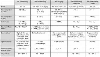
Figure 9. Feasible observations with current instrumentation. The table summarises the kind of objects and disk regions that can be currently probed with the available instrumentation, depending on their distances, stellar, and disk properties.
As very detailed observations of many disks start being a reality, finding common points between disks, and connecting observations either as results from the same physical process (with different initial conditions) or as different time-steps on initially similar objects will be also part of the analysis and interpretation of disks. From what we have learned from unresolved observations, the evolution/structure connection may not be evident nor immediate, so observing statistically significant samples will become a necessity. Future telescopes will also help in this direction by improving efficiency and sensitivity, allowing us to connect what we can observe in bright, nearby objects and fainter ones (including low-mass and solar-type stars, as well as more evolved disks). This will help to understand disks in their full range of stellar mass and time evolution.
Similarly, better models that allow for 3D disk structures will become more and more needed due to the increasing availability of spatially resolved observations. Although the present paper does not address the complex disk chemistry, high-sensitivity, and spatial resolution of molecular line observations will be an additional powerful tool to explore disks (see Haworth et al. Reference Haworth2016 on challenges for disks modellers).
8 CONCLUSIONS
In this paper, we explore the power of combined multi-wavelength observations to unveil details of protoplanetary disks that remain hidden, or are degenerated, when observed with a single technique. We show that combinations of observations can be used to remove the degeneracy in the interpretation of the disk structure, to distinguish disks with different structures, and to explore the paths of disk evolution. Well-devised, combined observations, even those with relatively old facilities, can help to unveil details of disks that are beyond the reach even of the most modern telescopes, also contributing to make the most with current ground- and space-based instrumentation.
The power of multi-wavelength data is also an indication that future advances will need to involve many experts working on different techniques. Our proposed Disk’s Rosetta Stone explores useful combinations of observations depending on the particular problem that we want to address, helping to devise time- and telescope-efficient observing schemes. The Disk’s Rosetta Stone is an ever-growing scheme: Our study is not complete and disk decryption will improve as new observations become feasible and gain sensitivity, power, efficiency, and time baseline.
ACKNOWLEDGEMENTS
We thank the organisers of the Protoplanetary Discussions in Edinburgh, 2016 March, and in particular, P. Woitke, for bringing all of us together and making possible this observational collaboration, and also for his comments to the paper. We also thank M. Benisty for her comments and suggestions and her participation in the discussion, D. Price for his support of this paper, B. López for his input regarding MIDI, and the anonymous referee for valuable comments that contributed to clarify this work. This work is the fruit of a collaborative effort between disk observers that use different observing techniques. A.S.A. is the organiser of the paper contributing to Sections 2, 5, 6. She also organised Section 7, to which all authors have contributed. A.B. is the co-organiser of the paper, leading Sections 2 and 3 and contributing to Section 7 and to the overall structure of the paper. A.C. and M.K. contributed to Sections 2 and 3. M.K is also the main contributor to Section 4. T. S. and A.G. led the scattering light and polarisation observations in Section 3. I.M. is the main contributor to accretion in massive stars in Section 5 and also contributed to Section 6. K.F. contributed to the disk dynamics part in Section 6. N.v.d.M. is the main contributor to the mm continuum interferometry part in Section 3. J.G. contributed to the dust mass part in Section 4. All authors contributed to the discussion in Section 7, as well as in building the Disk’s Rosetta Stone in Figures 8 and 9. This research has made use of NASA’s Astrophysics Data System.