


1. Introduction
Transfer of gases across a gas–liquid interface is of fundamental importance in many research fields, such as civil engineering and environmental science. Examples of interfacial gas exchange processes in nature include the absorption of climate controlling gases into the ocean, e.g. carbon dioxide, for which the ocean acts as a gigantic buffer, and the absorption of oxygen (reaeration) into rivers and streams, which is crucial for aquatic life. The transfer rate is governed by a variety of processes, the most important being the hydrodynamic flow conditions at the liquid side, which are significantly affected by the surface conditions. The latter includes surface contamination effects (e.g. Tsai & Liu Reference Tsai and Liu2003; McKenna & McGillis Reference McKenna and McGillis2004; Wissink et al. Reference Wissink, Herlina, Akar and Uhlmann2017), surface roughness effects (e.g. Turney Reference Turney2016) and whitecap effects (e.g. Brumer et al. Reference Brumer, Zappa, Blomquist, Fairall, Cifuentes-Lorenzen, Edson, Brooks and Huebert2017; Jähne Reference Jähne2020). In nature, turbulent flow typically generated by wind shear, buoyancy and/or bottom shear enhances the gas transfer rate. Wind shear is usually the most effective driving mechanism and has been extensively studied (e.g. Plate & Friedrich Reference Plate and Friedrich1984; Komori, Nagaosa & Murakami Reference Komori, Nagaosa and Murakami1993; Wanninkhof et al. Reference Wanninkhof, Asher, Ho, Sweeney and McGillis2009; Garbe et al. Reference Garbe2014). Furthermore, Tsai et al. (Reference Tsai, Chen, Lu and Garbe2013) and Turney (Reference Turney2016) found that at relatively low wind speeds Langmuir circulations (which are somewhat similar to very large-scale motions (VLSM) in open channel flow) contribute significantly to interfacial mass transfer. Also, with reducing wind speed, buoyancy and bottom-shear induced turbulence become increasingly important. Particularly in deep water bodies, buoyancy effects due to surface cooling (e.g. by evaporation) often contribute significantly to the interfacial transfer of heat and greenhouse gases (e.g. Podgrajsek, Sahlee & Rutgersson Reference Podgrajsek, Sahlee and Rutgersson2014). In rivers or streams, bottom shear induced turbulence is generally the dominant gas transfer mechanism, which we aim to study here in detail. To this end, highly accurate direct numerical simulations (DNS) of mass transfer across a shear-free surface in isothermal open channel flow were performed.
Commonly, the mass transfer across the air–water interface is measured using the transfer velocity  $K_L$, which remains difficult to predict accurately. Firstly, because of the complex interrelated physical processes (including molecular diffusion, turbulent mixing, waves and surfactants) and secondly, due to the fact that the interfacial transfer processes of low (O $_2$, CO, CH $_4$) to moderate (CO $_2$) soluble gases are concentrated in a very thin boundary layer on the water side adjacent to the surface (Jähne & Haußecker Reference Jähne and Haußecker1998). Thus, traditional empirical models for the prediction of gas transfer in streams and rivers are mostly based on global hydraulic parameters, such as water depth, bulk velocity and bottom slope (e.g. Thackston & Krenkel Reference Thackston and Krenkel1969; Gulliver & Halverson Reference Gulliver and Halverson1989) or more specific parameters, such as bed roughness (e.g. Moog & Jirka Reference Moog and Jirka2002).
Apart from empirical models, several conceptual models have also been proposed. An overview of several important conceptual models, such as the surface renewal model (Danckwerts Reference Danckwerts1951), the large-eddy model (Fortescue & Pearson Reference Fortescue and Pearson1967), the small-eddy model (Banerjee, Scott & Rhodes Reference Banerjee, Scott and Rhodes1968; Lamont & Scott Reference Lamont and Scott1970) and the surface divergence model (McCready, Vassiliadou & Hanratty Reference McCready, Vassiliadou and Hanratty1986) can be found in, for example, Theofanous (Reference Theofanous1984) and Herlina & Wissink (Reference Herlina and Wissink2014). Field measurements in various systems (including the coastal ocean and the large tidal freshwater river) by Zappa et al. (Reference Zappa, McGillis, Raymond, Edson, Hintsa, Zemmelink, Dacey and Ho2007) support the small-eddy model. By performing experiments in open channels, Plate & Friedrich (Reference Plate and Friedrich1984) and Moog & Jirka (Reference Moog and Jirka1999) showed the applicability of the small-eddy model to predict interfacial mass transfer. More recently, Turney & Banerjee (Reference Turney and Banerjee2013) experimentally validated the surface divergence model and showed that it can accurately predict open channel mass transfer in windless conditions. In contrast, for locally accelerating open channel flow, Sanjou (Reference Sanjou2020) observed that the constant of proportionality of the surface divergence model needs to be increased continuously (compared with non-accelerating flow) to account for the significant increases in mass transfer velocity due to the local acceleration.
The very thin concentration boundary layer mentioned above makes it very difficult to perform measurements (Herlina & Jirka Reference Herlina and Jirka2008) as well as fully resolved numerical simulations at realistic Reynolds and Prandtl / Schmidt numbers ( $Pr=\nu /\kappa _h$, $Sc=\nu /D$, where $\nu$ is the kinematic viscosity, $\kappa _h$ is the thermal diffusivity and $D$ is the molecular diffusivity). The main problem here is the very low diffusivity (high $Sc$) of many atmospheric gases in water, resulting in filaments with very large concentration gradients that need to be fully resolved. For this reason, DNS were usually performed at low to moderate Schmidt and/or Reynolds numbers. For example, Lakehal et al. (Reference Lakehal, Fulgosi, Yadigaroglu and Banerjee2003) and Tsai et al. (Reference Tsai, Chen, Lu and Garbe2013) performed DNS of interfacial mass transfer driven by surface-shear/wind for $Sc$ up to $10$ and $7$, respectively, while Schwertfirm & Manhart (Reference Schwertfirm and Manhart2007) performed DNS of buoyancy-driven mass transfer for $Sc$ up to $49$. Recently, DNS of highly realistic Schmidt numbers (e.g. $Sc \approx 500$ for O $_2$ and $Sc\approx 600$ for CO $_2$ in water) have been performed in buoyancy-driven flow by Wissink & Herlina (Reference Wissink and Herlina2016), Fredriksson et al. (Reference Fredriksson, Arneborg, Nilsson, Zhang and Handler2016) and in isotropic-turbulence driven flow by Herlina & Wissink (Reference Herlina and Wissink2014) and Herlina & Wissink (Reference Herlina and Wissink2019). Note that the latter is often used to produce a near-surface turbulent flow field that, despite the lack of streamwise anisotropy, is used to mimic the flow field generated by bottom shear, such as in open channel flow.
Handler et al. (Reference Handler, Saylor, Leighton and Rovelstad1999) were among the first to perform DNS of interfacial mass transfer in open channel flow, using a Prandtl number of  $Pr=2$ and a friction Reynolds number of $Re_\tau =u_\tau H/\nu = 180$, where $u_\tau$ is the friction velocity and $H$ is the channel height. It was observed that hairpin vortices were the dominant structures contributing to transfer of passive scalars in open channel flow. Nagaosa & Handler (Reference Nagaosa and Handler2003), who performed DNS for $Re_\tau = 150, 300$ and $Pr=1$, showed that these hairpin vortices, which were generated at the bottom wall, evolved into ring-like vortices as they approached the free surface. These ring-like vortices were observed to be present immediately below high mass transfer regions. Kermani et al. (Reference Kermani, Khakpour, Shen and Igusa2011) performed DNS at $Re_\tau \simeq 300$ and $0.71\le Sc \le 8$ and focused on the quantification of the surface age (i.e. the time between two surface renewal events). They concluded that Danckwerts’ assumption of a constant renewal rate does not apply at small (young) surface age, where interfacial mass transfer is actually at its largest. More recently, Nagaosa & Handler (Reference Nagaosa and Handler2012) performed DNS in open channel flow for $150\le Re_\tau \le 600$ with $Sc=1$. They evaluated the suitability of two characteristic time scales to approximate the renewal time in Danckwert's model. The first was based on the characteristic length and velocity scales at the free surface, while the other was the reciprocal of the root mean square (r.m.s.) of the surface divergence. Both time scales were found to perform well. Magnaudet & Calmet (Reference Magnaudet and Calmet2006) used the computationally less demanding large-eddy simulation (which only resolves the larger scales of motion) to be able to study interfacial mass transfer in open channel flow at a high friction Reynolds number of $Re_\tau =1280$ and Schmidt numbers ranging from $Sc=1$ to $200$. They confirmed the scaling of $K_L$ with $Sc^{-0.5}$ and found that the mass transfer was mostly driven by motions with a large streamwise extent.
In summary, because of the huge computational demands to fully resolve all scales of motion, previous DNS of interfacial mass transfer in open channel flow had the following limitations. (i) The DNS were limited to Schmidt numbers up to  $Sc=8$ which is approximately two orders of magnitude lower than the typical values encountered for atmospheric gases. (ii) With the exception of the $Re_\tau = 400$ and $600$ cases by Nagaosa & Handler (Reference Nagaosa and Handler2012), all other DNS were performed for $Re_\tau \leq 300$. Typically, with increasing $Re_\tau$ the range of scales present in the turbulence spectrum widens, which potentially changes the dominant physical mechanisms that play a role in interfacial mass transfer. (iii) The widening of the turbulent spectrum is not only directed towards the higher end, but also towards the lower end of the wavenumbers, as evidenced by the occurrence of VLSM, which has been observed both experimentally and numerically for sufficiently large $Re_\tau$ (e.g. Wang & Richter Reference Wang and Richter2019; Peruzzi et al. Reference Peruzzi, Poggi, Ridolfi and Manes2020). So far, in previous DNS of open channel flow with interfacial mass transfer, the size of the computational domain was often insufficient to accommodate the possible occurrence of VLSM. Hence, despite the valuable insights gained from previous DNS, the potential influence of VLSM on interfacial mass transfer has yet to be explored. Hence, there is good reason to perform further DNS using sufficiently large computational domains with flat, clean surfaces. The latter facilitates a highly accurate resolution of the near surface flow and scalar dynamics without significantly increasing the need for computational resources, which would otherwise severely restrict Reynolds and/or Schmidt number and/or domain size.
The series of DNS presented in this paper constitutes a significant leap forward by pushing the boundaries of both Reynolds and Schmidt numbers to  $180 \leq Re_\tau \leq 630$ and $7\leq Sc \leq 200$, respectively, as well as ensuring that the domain size was large enough to accommodate even the largest scales of motion that may occur in open channel flow. This was made possible due to the recent increases in computational power and the availability of the dual-meshing strategy in our KCFlo code (Kubrak et al. Reference Kubrak, Herlina, Greve and Wissink2013), which also allows us to simultaneously solve multiple scalar transport equations. The above enables us to numerically explore the physical mechanisms that control interfacial mass transfer in the presence of VLSM at high Schmidt numbers. This includes, for instance, (i) the confirmation that the $Sc^{-0.5}$ scaling of the transfer velocity for larger Schmidt numbers also holds in open channel flow; (ii) investigating the importance of turbulence dissipation on local mass transfer in the presence of VLSM; (iii) evaluating the validity of Theofanous’ model for open channel flow mass transfer; and (iv) producing benchmark data on near surface scalar statistics that can be used for improvement and/or development of new mass transfer models, for example predictive climate change simulations.
2. Numerical aspects
2.1. Numerical method
The mathematical formulation describing the process of mass transfer (e.g. dissolved gas transfer) in turbulent open channel flow comprises the incompressible Navier–Stokes equations for the flow and advection–diffusion equations for the scalar concentration field, which in non-dimensional form read
 \begin{gather} \dfrac{\partial u^*_i}{\partial x^*_i} = 0, \end{gather}
 \begin{gather} \dfrac{\partial {u^*_i}}{\partial t^*}+\dfrac{\partial u^*_i u^*_j}{\partial x^*_j} ={-}\dfrac{\partial p^*}{\partial x^*_i} +\dfrac{1}{Re_b} \dfrac{\partial ^2 u^*_i}{\partial x^*_j \partial x^*_j} + f^*\delta_{i1}, \end{gather}
 \begin{gather} \dfrac{\partial c^*}{\partial t^*}+\dfrac{\partial u^*_jc^*}{\partial x^*_j} =\dfrac{1}{Re_b\,Sc} \dfrac{\partial ^2 c^*}{\partial x^*_j \partial x^*_j}, \end{gather}
where  ${\phi }^*$ denotes the non-dimensional form of $\phi$, $(u_1, u_2, u_3) = (u, v, w)$ are the velocity components in the $(x_1,x_2,x_3) = (x, y, z)$ direction, respectively, $t$ is time, $p$ is pressure, $\delta$ is the Kronecker delta, $f$ is the dynamically adjusted forcing term added to the momentum equation to ensure a constant flow rate, $c$ is the scalar concentration and $Sc$ is the Schmidt number. The bulk Reynolds number is defined as $Re_b=U_b H/\nu$, where $H$ is the height of the channel and $U_b$ is the bulk velocity. The latter is defined by $U_b =({1}/{H})\int ^H_0 \overline {\langle {u}\rangle }\,{\rm d}{y}$, where $\bar {\cdot }$ and $\langle \cdot \rangle$ denote averaging over time and the homogeneous horizontal ( $x,z$) directions, respectively. Note that for a fully developed turbulent flow changes in $f$ are negligibly small. The scalar concentration is normalised by
 \begin{equation} c^*=\frac { {c}-{c}_{b,0}} {{c}_s-{c} _{b,0} }, \end{equation}
where  ${c}_{b,0}$ is the initial concentration in the bulk and ${c}_{s}$ is the saturation concentration at the surface.
The full set of governing equations was solved using the in-house KCFlo code (Kubrak et al. Reference Kubrak, Herlina, Greve and Wissink2013). The momentum equations were discretised using a fourth-order central scheme for diffusion combined with a fourth-order kinetic energy conserving scheme for convection. The Poisson equation for the pressure was solved using a conjugate gradient solver, with simple diagonal preconditioning. The scalar advection–diffusion equations were discretised using a fifth-order weighted essentially non-oscillatory scheme (Liu, Osher & Chan Reference Liu, Osher and Chan1994) for the convection, and a fourth-order accurate central scheme for the diffusion. As the scalar diffusivities are much smaller than the momentum diffusivity, a dual-mesh approach (using a finer mesh for the scalar computation than for the flow computation) was used in order to accurately resolve the Batchelor scales in a computationally efficient manner.
The solutions of both flow and scalar fields were advanced in time using the second-order accurate explicit Adams–Bashforth scheme. Three scalar advection–diffusion equations with different Schmidt numbers were solved simultaneously, enabling a direct comparison of scalar transport processes driven by exactly the same background turbulence.
The constitutive parts of our numerical code were validated in Wissink (Reference Wissink2004) for the flow solver and in Kubrak et al. (Reference Kubrak, Herlina, Greve and Wissink2013) for the scalar advection–diffusion. In the latter reference, the numerical treatment of the scalar transport process was compared with analytical solutions for pure advection as well as pure diffusion, and the convergence rate of the method was rigorously established. Furthermore, the effectiveness and convergence of our dual-meshing approach was demonstrated in, for example, Kubrak et al. (Reference Kubrak, Herlina, Greve and Wissink2013), Herlina & Wissink (Reference Herlina and Wissink2014) and Wissink & Herlina (Reference Wissink and Herlina2016).
2.2. Computational set-up
As mentioned above, the present study focuses on low diffusivity mass transfer in a fully developed turbulent open channel flow. The size of the computational domain was  $L_x\times L_y \times L_z$ in the streamwise ( $x$), vertical ( $y$) and spanwise ( $z$) directions, respectively (cf. figure 1). Three different domain sizes were used: $3H\times H\times 3H$, $12H\times H\times 3H$ and $24H\times H\times 6H$. The total number of grid points employed in the simulations ranged from $4.72\times 10^6$ to $1.22\times 10^{10}$. The Schmidt and bulk Reynolds numbers were varied from $Sc=4$ to $200$ and $Re_b=2875$ to $12\,000$, respectively. A list of the simulations performed is provided in table 1.

Figure 1. Schematic of the computational domain.
Table 1. Overview of the simulations. Here  $Re_b$ is the bulk Reynolds number, $Re_\tau$ is the friction Reynolds number, $Sc$ is the Schmidt number, $H$ is the channel height, $L_x \times L_y \times L_z$ denote the size of the domain in $x,y,z$ directions, respectively, $N_x, N_y, N_z$ are the number of grid points in the base mesh, while $\psi _x, \psi _y, \psi _z$ denote the refinement factors used for the finer scalar mesh (of the $Sc$ cases marked with superscript $R$) and $\Delta t_f /t_b$ is the time window used for the flow statistics, where $t_b=H/U_b$ is the bulk time unit. Note that the time window of the scalar statistics differ from $\Delta t_f /t_b$, as will be explained in § 4.2.

In all simulations, the surface was assumed to be flat, thereby neglecting any possible influence of waves on mass transfer. For both flow and scalar fields, periodic boundary conditions were used in the streamwise and spanwise directions. In the vertical direction, a free-slip boundary condition at the free surface ( $y/H=1$) and a no-slip boundary condition at the wall ( $y/H=0$) of the channel were applied for the velocity field. For the scalars, at the surface a Dirichlet boundary condition with $c=c_s$, modelling the presence of the atmosphere was employed, while at the wall a zero flux boundary condition ( $\partial c/ \partial y = 0$) was used. To speed up the formation of a turbulent concentration boundary layer, the concentration field was initialised using the solution of the unsteady diffusion equation (cf. e.g. Fischer et al. Reference Fischer, List, Koh, Imberger and Brooks1979)
 \begin{equation} c^*(1-y/H)=\text{erfc}\left(\frac{1-y/H}{\sqrt{{4t_d^*}/{(Re_bSc)}}}\right), \end{equation}
for a prescribed non-dimensional diffusion time  $t_d^*$, which was set to $10$ for the smallest domain considered and $12$ for the two larger domains.
The spatial discretisation was performed on a non-uniform and staggered Cartesian mesh. The mesh was uniform in the homogeneous ( $x$,
$x$,  $z$) directions and stretched in the vertical ( $y$) direction with refinement near the free surface, located at $y(N_y)=H$, and the wall, located at $y(0)=0$. The node distribution is given by
 \begin{equation} y(k) = \left[1-\frac{\tanh(y_\phi)}{\tanh(y_1)}\right]\frac{y(0)}{2} + \left[1+\frac{\tanh(y_\phi)}{\tanh(y_1)}\right]\frac{y(N_y)}{2} \end{equation}
for  $k=1,\ldots,N_y-1$, with
 \begin{gather} y_1=\psi_m/2, \end{gather}
 \begin{gather}y_{\phi}=\psi_m \left[\frac{k}{N_y}-0.5\right], \end{gather}
where  $N_y$ is the number of nodes in the $y$ direction. The stretching is controlled by the parameter $\psi _m = ({k}/{N_y}) \psi _t + [1-{k}/{N_y}]\psi _b$, where $(\psi _t, \psi _b)$ was set to $(2, 2)$ in the smallest domain, $(3, 2)$ in the midsized domain and $(2.3, 3)$ in the largest domain. The adequacy of the base mesh resolution for all simulations was confirmed by studying one-dimensional (1-D) energy spectra of the velocity, as discussed in § 3.1.
As mentioned above, a dual-mesh strategy was employed to accurately resolve the evolution of the high  $Sc$ scalar fields. The refined grid resolution was chosen such that (i) the vertical grid size $\Delta y$ at the surface was less than $0.15L_B$, where $L_B=\eta /\sqrt {Sc}$ is the Batchelor scale and $\eta$ is the Kolmogorov scale; and (ii) the geometric mean of the grid cells $\Delta =\sqrt [3]{\Delta x\Delta y \Delta z}$ was $\Delta <{\rm \pi} \,L_B$ in the upper part of the domain ( $y/H \le 0.55$). These two conditions fulfil the criterion proposed by Grötzbach (Reference Grötzbach1983), which ensures that the scalar mass transfer in all simulations is adequately resolved.
2.3. Domain size
Before proceeding with the discussion of the results, a brief overview of the effect of the domain size on the flow structures in open channel flow is presented. A more detailed investigation can be found in, for example, Wang, Park & Richter (Reference Wang, Park and Richter2020), while similar investigations for closed channel flow were carried out by, for example, Hwang & Cossu (Reference Hwang and Cossu2010), Lozano-Durán & Jiménez (Reference Lozano-Durán and Jiménez2014), Feldmann, Bauer & Wagner (Reference Feldmann, Bauer and Wagner2018) and Abe, Antonia & Toh (Reference Abe, Antonia and Toh2018).
One of the main findings reported in the investigations mentioned above is the appearance of very large coherent structures for large  $Re_\tau$. To assess the suitability of the domain sizes used in the present simulations for capturing such large coherent structures, typical snapshots of the streamwise velocity fluctuations $u^\prime$ at $y/H=0.6$ for G03, G06, G09 are shown in figures 2(a), 2(c) and 2(e), respectively. As can be seen in table 1, these cases have the highest $Re_\tau$ for each of the three domain sizes considered. In all figures, high and low velocity elongated streaky structures, that are characteristic of open-channel flow, can be seen. The snapshots and corresponding two-point correlations
 \begin{gather} {\mathsf{R}}_{uu}^x(\Delta x,y)=\overline{\left ( \frac{\langle u^\prime(x,y,z,t) u^\prime(x+\Delta x,y,z,t) \rangle} {\langle u^\prime(x,y,z,t)^2 \rangle} \right)}, \end{gather}
 \begin{gather}{\mathsf{R}}_{uu}^z(\Delta z,y)=\overline{ \left ( \frac{\langle u^\prime(x,y,z,t) u^\prime(x,y,z+\Delta z,t) \rangle} {\langle u^\prime(x,y,z,t)^2 \rangle} \right)}, \end{gather}
at  $y/H=0.6$ (figure 2b,d,f) indicate that the streamwise extent of these coherent structures was captured quite well in the largest domain and marginally in the midsized domain, but not in the smallest domain.

Figure 2. Instantaneous contour maps of  $u^\prime /U_b$ (a,c,e) and time-averaged two-point correlations $R_{uu}$ of the streamwise velocity (b,d,f) in the plane $y/H = 0.6$ for simulations performed (a,b) in the small $3H\times H\times 3H$ domain at $Re_\tau = 290$, (c,d) in the midsized $12H\times H\times 3H$ domain at $Re_\tau = 290$ and (e,f) in the large $24H\times H\times 6H$ domain at $Re_\tau = 630$. The lines in (b,d,f) represent ${\mathsf{R}}_{uu}$ in streamwise (solid lines) and spanwise (dashed lines) directions.
For both  $Re_\tau =365$ and $630$, the proper decorrelation of $u^\prime$ in the largest domain (shown for $Re_\tau =630$ and $y/H=0.6$ in figure 2f) was achieved in the spanwise direction for all $y/H$ and in the streamwise direction for $y/H \leq 0.7$. For $y/H>0.7$ the minimum value for the streamwise ${\mathsf{R}}_{uu}$ was always smaller than $0.05$, indicating a more marginal decorrelation. Therefore, we can assume that the $24H\times H \times 6$ domain size was sufficiently large to effectively capture the VLSM for $Re_\tau$ up to $630$. In contrast, for the lowest $Re_\tau =200$, a decorrelation of $u^\prime$ in both horizontal directions was obtained for the entire depth. In the midsized simulations, the streamwise decorrelation was marginal for all cases, while in the smallest domain no decorrelation was achieved. As expected, a domain size of $3H \times H \times 3H$ is too small to fully capture turbulent open-channel flow, even for $Re_\tau$ as low as $190$. Nevertheless, it will be shown in § 4.1 that for $Re_\tau = 240$ and $290$ the interfacial mass transfer was found to be largely independent of the domain size.
Furthermore, in figure 2(e) coherent structures of lengths roughly  $10H$ and $20H$ can be seen. In the literature, structures of length $\gtrsim 10H$ are usually referred to as VLSM, while the term large-scale motions (LSM) is typically used for structures with a length of $\approx 1-3H$. In open channel flow, the onset of the appearance of VLSM is still uncertain (cf. e.g. Adrian & Marusic Reference Adrian and Marusic2012). To date such motions have been confirmed to appear for $Re_\tau \ge 550$ (Wang & Richter Reference Wang and Richter2019) and experimentally at $Re_\tau \geq 700$ (Peruzzi et al. Reference Peruzzi, Poggi, Ridolfi and Manes2020). The very large coherent structure seen in figure 2(e) is an example of such a VLSM that is found at $Re_\tau =630$. Later it will be shown that in the present simulations VLSM could already be detected at $Re_\tau = 365$. Further confirmation of the appearance of VLSM based on, for example, premultiplied spectra and velocity fluctuations analyses, is presented in § 3.1.
3. Flow characteristics
3.1. Flow statistics
All simulations were started from fully developed turbulent flow fields. The shown statistics, if not stated otherwise, were obtained by averaging in the homogeneous ( $x$,
$x$,  $z$) directions and in time (cf. table 1).
Figure 3(a) shows that the mean streamwise velocity profiles in all simulations agree well with the law of the wall, including a logarithmic region  $u^+=({1}/{\kappa })log(y^+)+B$, with standard values for the von Kármán constant ( $\kappa =0.40$) and for the intercept ( $B=5$). The 1-D streamwise energy spectra of the velocity components for the simulation with the largest Reynolds number (G09) are shown in figure 3(b). As also observed for all other simulations, the existence of an inertial subrange, indicated by the $k^{-5/3}$ power law, can be clearly seen. Furthermore, no energy pile-up at high wavenumbers was observed, demonstrating that the smallest scales of motion were well resolved in all simulations. In addition, it was found that $Re_\tau =0.166Re_b^{0.88}$, which is in agreement with the results for closed channel flow as shown by Pope (Reference Pope2000) and Lee & Moser (Reference Lee and Moser2015).

Figure 3. (a) Near-wall mean streamwise velocity profiles: blue solid line, G01; blue dashed line, G02; blue dotted line, G03; red solid line, G04; red dashed line, G05; red dotted line, G06; black solid line, G07; black dashed line, G08; black dotted line, G09; teal solid line,  $u^+=y^+$; teal dashed line, the logarithmic law with $\kappa =0.40$ and $B=5$. (b) The 1-D energy spectra in streamwise direction from simulation G09 at $y/H=0.7$.
Figure 4 shows contours of the longitudinal velocity fluctuation spectra in the streamwise ( $x$) and the spanwise ( $z$) directions from the simulations performed in the $24H \times H \times 6H$ domain (G07–G09). The energy spectra were premultiplied by the wavenumber and are shown as a function of the wavelength and distance from the wall. As expected, for increasing Reynolds number the amount of energy at smaller wavelengths was found to increase, especially near the wall of the channel. Higher up in the boundary layer (for $y/H > 0.2$) all streamwise spectra (figure 4a–c) show an energy peak at a wavelength of $\lambda _x/H \approx 3$. This peak is associated with LSM. It should be noted that in the spectra, the location of the peaks with higher wavelengths becomes less accurate due to the limited size of the computational domain $L_x=24H$, $L_z=6H$. Even though the location may not be entirely correct, the energy peaks observed at $\lambda _x \gtrsim 10H$, which extend over virtually the whole channel height, indicate the presence of VLSM for $Re_\tau \ge 365$ (G08, G09). When examining the spanwise spectra (figure 4d–f), energy peaks at $\lambda _z/H \approx 1$, which relate to LSM, were detected in all three cases. High energy values at $\lambda _z/H \ge 2$ (typical for VLSM) were observed for $Re_\tau =365$ and $Re_\tau =630$ when $y/H\ge 0.3$ and $0.1$, respectively.

Figure 4. Contour maps of normalised premultiplied longitudinal velocity fluctuation spectra in (a–c) streamwise ( ${\mathsf{E}}^*_{u'u'}=k_x\,{\mathsf{E}}_{u'u'}/(k_x\,{\mathsf{E}}_{u'u'})_{max}$) and (d–f) spanwise ( ${\mathsf{E}}^*_{w'w'}=k_z\,{\mathsf{E}}_{w'w'}/(k_z\,{\mathsf{E}}_{w'w'})_{max}$) directions as a function of wavelength and distance from the wall ( $y/H$). The Reynolds numbers for the shown cases are (a,d) $Re_\tau =200$, (b,e) $Re_\tau =365$ and (c,f) $Re_\tau =630$.
The r.m.s. of the velocity fluctuations for the simulations performed using the midsized and large-sized domains are shown in figure 5. As expected, a decrease in the boundary layer thickness at the wall with increasing Reynolds number was observed. The increase in the peak of the streamwise component  $u_{rms}$ (figure 5a) from $2.7$ for $Re_\tau =200$ to $2.8$ for $Re_\tau =630$ is in good agreement with the values reported in Kim, Moin & Moser (Reference Kim, Moin and Moser1987), Pope (Reference Pope2000) and Wang & Richter (Reference Wang and Richter2019). For $y/H \ge 0.3$, the $u_{rms}^+$ profiles for $Re_\tau < 365$ were found to nearly collapse on one curve, while for $Re_\tau \ge 365$ the $u_{rms}^+$ profiles tend to grow with $Re_\tau$. This increase in $u_{rms}^+$ tends to be associated with the presence of VLSM (Kim & Adrian Reference Kim and Adrian1999; Del Álamo et al. Reference Del Álamo, Jiménez, Zandonade and Moser2004; Hoyas & Jiménez Reference Hoyas and Jiménez2006).

Figure 5. Profiles of r.m.s. velocity fluctuations normalised by the friction velocity  $u_\tau$ as a function of $y/H$. The lines represent: red solid line, G04; red dashed line, G05; red dotted line, G06; black solid line, G07; black dashed line, G08; black dotted line, G09.
Figures 5(b) and 5(c) show that for  $y/H \ge 0.3$, similar $v_{rms}^+$ profiles and similar $w_{rms}^+$ profiles were obtained for all Reynolds numbers. At the surface, vertical fluctuations are damped and the turbulent kinetic energy is redistributed in the horizontal directions, which explains the slight increase in $u^+_{rms}$ as well as the significant increase in $w^+_{rms}$ towards the surface. To the authors’ knowledge, previous experiments (e.g. Nezu & Rodi Reference Nezu and Rodi1986; Turney & Banerjee Reference Turney and Banerjee2013) do not show any conclusive proof either against or in support of such increases in $u^+_{rms}$ and $w^+_{rms}$. This is likely related to the fact that it is very difficult to maintain a perfectly clean surface while performing experiments, especially when using seeding particles as tracer. Such contamination was shown to result in near-surface turbulence damping (cf. e.g. McKenna & McGillis Reference McKenna and McGillis2004; Wissink et al. Reference Wissink, Herlina, Akar and Uhlmann2017). The thickness of the surface influenced layer $L_{s}$ was determined by the distance between the surface and the location, $y_\infty$, where $I(y)= \overline {( {\langle uu\rangle }+{\langle vv \rangle }+{\langle ww\rangle } ) / ( {\langle uu\rangle }+{\langle ww\rangle } )}$ is maximum ( $L_s = (H-y_\infty )$). Here $I$ can be seen as a measure of the Reynolds stress anisotropy, where the lower limit $I=1$ corresponds to two-dimensional flow, while isotropic flow would result in $I=3/2$. In open channel flow, the former is achieved at the free surface. With increasing distance from the surface ( $H-y > 0$), the flow becomes less anisotropic and hence the magnitude of $I$ increases until it reaches a maximum at the edge of the surface influenced layer ( $y=y_\infty$). Here, in all simulations, $y_\infty$ was found to be located somewhere between $0.6H$ and $0.75H$ (cf. table 2), such that $0.25H\leq L_s \leq 0.4H$. When comparing simulations of the same domain size, the surface influenced layer $L_s$ was found to decrease with increasing $Re_\tau$.
Table 2. Parameters used in the definition of the turbulent Reynolds number for the simulations listed in table 1. The location  $y_\infty$ identifies the edge of the surface influenced layer (cf. § 3.1), $L_{\infty }, u_{\infty }, Re_T$ are defined in (4.8). Note that all values were obtained by averaging over a time window $\Delta t_s/t_b$ in which the scalar statistics are quasisteady, see table 1.

Figure 6 shows the integral length scales for the velocity components in the homogeneous directions as a function of  $y/H$ for the largest domain size. For $y/H > 0.4$, a significant increase in the integral length scale in the $x$ direction ( $L_{uu}^x$ ) by approximately $50\,\%$ was observed when increasing the Reynolds number from $Re_\tau =200$ to $365$. Further increasing $Re_\tau$ to $630$ resulted in a further increase in $L_{uu}^x$ by approximately $10\,\%$ (figure 6a). This significant growth in $L_{uu}^x$ for $Re_\tau =365$ and $630$ corresponds to the presence of VLSM. For $y/H\leq 0.05$, all integral length scales in the $x$ direction ( $L_{uu}^x$, $L_{vv}^x$ and $L_{ww}^x$) can be seen to decrease with increasing Reynolds number. This trend persists for $L_{vv}^x$ for (almost) every $y/H$, and for $L_{ww}^x$ until $y/H\approx 0.8$. Compared with the $x$ direction, with the possible exception of $L_{ww}^z$, the integral length scales in the $z$ direction do not show any significant Reynolds number effect.

Figure 6. Integral length scales of the velocity components (a)  $u$, (b) $v$ and (c) $w$ in the $x$ direction (red) and $z$ direction (blue) as a function of $y/H$. The data are from the $24H \times H \times 6H$ domain simulations with $Re_\tau =200$ (solid lines), $Re_\tau =365$ (dashed lines) and $Re_\tau =630$ (dotted lines).
3.2. Flow structures
Figure 7 shows contours of the streamwise-averaged  $u$ fluctuation ( $\langle u^\prime /U_b \rangle _x$), together with streamwise-averaged velocity vectors of the two components in the plane. Large areas with high- and low-speed streamwise flow can be observed, which extend almost from the wall to the free surface of the channel. Downward moving flow is typically present in the high streamwise velocity areas, while in the low-speed areas the flow tends to move upwards. It was observed in figure 2(a) that these high- and low-speed areas extend over a significant streamwise portion of the channel, and are related to VLSM.

Figure 7. Typical contour plot of the streamwise averaged  $u$ fluctuation $\langle u^\prime /U_b \rangle _x$ from simulation G09 (at $t/t_b=52$). The black arrows represent the streamwise averaged velocity components in the cross-plane, ( $\langle v/U_b \rangle _x, \langle w/U_b \rangle _x$).
Figure 8(a) shows contours of streamwise velocity fluctuations  $u^\prime /U_b$ in the plane at $y/H=0.5$. Superimposed on this plot are small-scale vortical structures in the interval $0.5\leq y/H\leq 1$ that are visualised using the normalised $Q$-criterion,
 \begin{equation} q(x,y,z,t) = {Q(x,y,z,t)} / {Q_{rms}(y)}, \end{equation}
where  $Q$ is the second invariant of the velocity gradient tensor (Hunt, Wray & Moin Reference Hunt, Wray and Moin1988) and $Q_{rms}$ is the r.m.s. of $Q$ determined using temporal and spatial averaging in $x, z$. In figure 8(a), it can be seen that the vast majority of the small-scale vortical structures is present inside large low-speed streaks that extend toward the surface (cf. also figure 7). The strong concentration of these small structures in low-speed streaks can be explained as follows. Low-speed streaks form when relatively slow moving, highly turbulent flow from the lower part of the boundary layer is ejected to the upper, less turbulent part of the boundary layer (e.g. Komori et al. Reference Komori, Ueda, Ogino and Mizushina1982). This larger turbulence intensity is responsible for the concentration of small-scale structures observed inside the low-speed streaks.

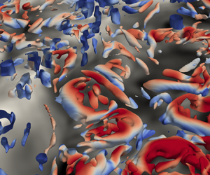
Figure 8. Typical vortical structures from simulation G09 (at  $t/t_b=52$), visualised by isosurfaces that correspond to a value of (a) $q=1$ and (b) $q=0.1$, see (3.1). In (a) the structures are coloured by $y/H$, while in (b) they are coloured by the fluctuating vertical velocity. The background contour map represents the streamwise velocity fluctuation in the $x$–
$x$– $z$ plane at (a) $y/H=0.5$ and (b) $y/H=0.9$.
When the small vortices approach the surface they either align with or become orthogonal to the surface, which are referred to as surface-aligned and surface-attached vortices, respectively. Figure 8(b) shows an instantaneous snapshot of the upper part ( $y/H\ge 0.9$) of the channel. Most of the surface-attached vortices were found above downwelling motions corresponding to high-speed streaks. As mentioned above, in low-speed streaks most of the vortical structures are present. These structures tend to align with the surface due to the shear generated underneath the divergent flow at the surface. In these low-speed regions, the surface-aligned vortices are often ring-shaped, which according to Nagaosa & Handler (Reference Nagaosa and Handler2003) started their life as hairpin vortices from near the wall of the channel.
The implications of the above on interfacial mass transfer will be discussed in § 4.4.
4. Mass transfer
4.1. Instantaneous results
Figure 9 shows typical contours of the concentration, and qualitatively depicts the interaction between the turbulent open channel flow and the scalar transport at  $Sc=7$ (a,c) and $Sc=100$ (b,d). The thickness of the concentration boundary layer $\delta$, which will be defined in (4.1), below, depends on both the Reynolds and the Schmidt number. Comparing the vertical cross-sections ( $x,y$ planes) shown in figures 9(a) and 9(b), it can be clearly seen that an increase in Schmidt number at constant $Re_b$ results in much finer concentration filaments in the bulk and a significantly reduced boundary layer thickness. Note that for a shear-free surface, the thickness $\delta$ scales with $Sc^{-0.5}$ (cf. figure 10a) so that $\delta _{Sc=7} \approx 3.78\delta _{Sc=100}$. This scaling is not taken into account in figures 9(c) and 9(d), which shows surface-parallel planes at a distance of $0.0003H$ to the surface, corresponding to $\simeq 0.019\delta$ and $\simeq 0.071 \delta$ for $Sc=7$ and $100$, respectively. Hence, the range of the scalar concentrations in figure 9(d) had to be increased by a factor of $\approx \sqrt {100/7}=3.78$ to obtain similar contours. Nevertheless, small differences can still be observed locally due to differences in diffusion in the horizontal directions.

Figure 9. Typical contours of  $c^*$ in the $x$–
$x$– $y$ plane (a,b) and in the $x$–
$x$– $z$ plane at $y/H=0.9997$ (c,d). Shown are snapshots from G07 (at $t/t_b=42$) for (a,c) $Sc=7$ and (b,d) $Sc=100$. Please note the different ranges in the colour maps of panes (c,d).

Figure 10. (a) Typical scaling of the mean boundary layer thickness  $\overline {\langle \delta \rangle }/H$ with $Sc$, shown here for case G07. Also included are: black solid line, the Kolmogorov scale ( $\overline {\langle \eta \rangle }/H$); black dotted line, the Batchelor ( $\overline {\langle L_B\rangle }/H$) scale; black dashed line, the $Sc^{-0.5}$ slope. (b) Normalised boundary layer thickness $\overline {\langle \delta \rangle }\sqrt {Sc}/H$ as a function of $Re_b$. The black dashed line represents $14.4Re_b^{-0.67}$.
Note that the above reduction in  $\delta$ at a fixed $Re_b$ is due to the increase in interfacial mass transfer resistance with increasing Schmidt number. At a fixed $Sc$, the increase in turbulence in the bulk associated with an increase in $Re_b$ results in improved mixing with a reduction of $\delta$, which in this case promotes mass transfer.
4.2. Statistics of scalar transport
As mentioned in § 3.1, all simulations were started from fully developed turbulent flow fields with the scalars initialised by (2.5). After a transient period needed to ensure that the scalar statistics were quasisteady, scalar averaging was carried out using a time window of  $\Delta t_s/t_b$ (see table 2).
The thickness of the diffusive concentration boundary layer  $\delta$ is identified using
 \begin{equation} \delta = \frac {(c_s-\overline{\langle c_b \rangle})}{ \partial c / \partial y|_{y=H}}. \end{equation}
As illustrated in figure 10(a) for simulation G07, in all simulations  $\delta$ was found to scale with $Sc^{-0.5}$, which is in agreement with the theoretical prediction for a shear-free interface (e.g. Ledwell Reference Ledwell1984). Included in this plot are the thicknesses of the Kolmogorov sublayer $\eta$ and the Batchelor sublayer $L_B$ at the interface. Except for $Sc=7$, it was found that $L_B < \delta < \eta$, which is in agreement with Herlina & Wissink (Reference Herlina and Wissink2014) (hereafter HW14).
Figure 10(b) shows the variation of  $\overline {\langle \delta \rangle } \sqrt {Sc}/H$ with the bulk Reynolds number $Re_b$. It can be seen that for $Re_b=4000$ and $5000$, the normalised boundary layer thickness is nearly independent of the computational domain size. The best fit through the data points was found to be $\overline {\langle \delta \rangle } \sqrt {Sc}/H \propto Re_b^{-0.67}$. This will be discussed further in § 4.3, where the scaling will be linked to the transfer velocity.
Figure 11 shows normalised mean vertical profiles of the concentrations, the r.m.s. of concentration fluctuations and the mass fluxes at various Reynolds numbers (G07, G08 and G09). As discussed above, the boundary layer thickness  $\delta$ depends on both the molecular diffusivity ( $Sc$) and the Reynolds number ( $Re_b$). Thus, it is expected that the vertical profiles of the normalised mean scalar quantities exhibit self-similarity when the vertical $(H-y)$ direction is normalised by $\overline {\langle \delta \rangle }$. (Note that the profiles for the different Schmidt numbers also collapse.)

Figure 11. Vertical profiles of normalised (a) mean concentration, (b) r.m.s. of concentration, (c) mean diffusive  $j_d/j_s$ and turbulent $j_t/j_s$ mass fluxes, where $j_s$ denotes the surface mass flux. Shown are profiles at $Sc=16$ for various bulk Reynolds numbers: $Re_b=3200$ (G07, solid lines), $Re_b=6400$ (G08, dashed lines) and $Re_b=12\,000$ (G09, dotted lines).
In all simulations, the magnitude of  $\overline {\langle \delta \rangle } /H$ was found to be virtually identical to the distance between the surface and the location at which the r.m.s. of the concentrations
 \begin{equation} c_{rms} = \sqrt{\overline{\langle c^2 \rangle - \langle c \rangle^2}} \end{equation}
reaches its maximum. Hence, the peak in figure 11(b) is located at  $(H-y)/\overline {\langle \delta \rangle }=1$. The maximum $c_{rms}/(c_s-c_b)$ values were $\approx 0.3$, which is in agreement with previous numerical (Magnaudet & Calmet Reference Magnaudet and Calmet2006; Herlina & Wissink Reference Herlina and Wissink2014, Reference Herlina and Wissink2019) and experimental (Atmane & George Reference Atmane and George2002) results. The lower normalised $c_{rms}$ peak values of ${\approx }0.1\text {--}0.2$ obtained in the experiments of Herlina & Jirka (Reference Herlina and Jirka2008) and Janzen et al. (Reference Janzen, Herlina, Jirka, Schulz and Gulliver2010) indicate a partially contaminated surface, as confirmed by the numerical studies of Khakpour, Shen & Yue (Reference Khakpour, Shen and Yue2011) and Wissink et al. (Reference Wissink, Herlina, Akar and Uhlmann2017).
The total averaged vertical mass flux,  $j=j_d +j_t$, comprises a diffusive component
 \begin{equation} j_d(y)={-}D \frac{\partial \overline{\langle c \rangle}}{\partial {y}} \end{equation}
and a turbulent component
 \begin{equation} j_t(y)=\overline{\langle c^\prime v^\prime \rangle}. \end{equation}
 Figure 11(c) illustrates that  $j_d$ dominates at the surface, as $v'$ is damped due to the two-dimensionality imposed by the free-slip boundary condition. With increasing distance to the surface the contribution of $j_d$ to the total mass flux reduces, while at the same time the contribution of $j_t$ becomes increasingly important until it entirely dominates $j$. It can also be seen that at $(H-y)/\overline {\langle \delta \rangle }\simeq 0.65$ the diffusive and turbulent mass fluxes become equal. Furthermore, it was found that in the range $2\lessapprox (H-y)/\overline {\langle \delta \rangle }\lessapprox 10$, the turbulent mass flux $\overline {\langle c'v' \rangle }$ agrees reasonably well with the mass flux at the surface ( $j_s$).
From the surface ( $y=H$) down to a depth of $(H-y)\approx 2\overline {\langle \delta \rangle }$, the normalised mean vertical profiles of the scalar quantities shown in figure 11 were found to nearly collapse with the profiles reported in Herlina & Wissink (Reference Herlina and Wissink2019), hereafter HW19 (not included in the plot), where the interfacial mass transfer was driven by isotropic turbulence diffusing upwards from the opposite boundary. For the highest Reynolds number case (G09), the agreement between the open channel profiles produced here and in the case driven by isotropic turbulence remains reasonably well up to a distance of at least $10\overline {\langle \delta \rangle }$ from the free surface. This indicates that the strong anisotropy present in the velocity field of turbulent open channel flow (which increases with increasing Reynolds number) does not affect the shape of the normalised profiles at least up to the aforementioned depth.
4.3. Scaling of mass transfer velocity
The local, instantaneous transfer velocity  $k_l$ is defined as
 \begin{equation} k_l (x,z,t) =\left| {\frac{-D\left. {\partial c(x,z,t)}/{\partial y} \right |_{y=H} } { c_s- \langle c_b \rangle }} \right|. \end{equation}
For open channel flow with no wind shear, the mean transfer velocity
 \begin{equation} K_L = \left| \frac{\left. j_d\right |_{y=H}}{c_s-\overline{\langle c_b \rangle}}\right| = \langle \overline{k_l(x,z,t)} \rangle, \end{equation}
is commonly parameterised using the bulk Reynolds number  $Re_b$ or the friction Reynolds number $Re_\tau$. In figure 10 it was found that $\overline {\langle \delta \rangle /H}$ scales with $Sc^{-0.5}$ and $Re_b^{-0.67}$. Hence, as
 \begin{equation} \overline{\langle \delta \rangle} =D/K_L, \end{equation}
the normalised transfer velocities  $K_L/U_b$ obtained here scale with $Sc^{-0.5}$ and $Re_b^{-0.33}$. The former scaling was found to be valid only for clean (surfactant-free) surfaces (Wissink et al. Reference Wissink, Herlina, Akar and Uhlmann2017). The power $n=-0.33$ in the latter scaling is somewhat smaller than the one found in the DNS of Nagaosa & Handler (Reference Nagaosa and Handler2012), hereafter NH12, who obtained $K_L \propto Re_b^{-0.25}$ in small-box simulations at $Sc=1$. When using the friction Reynolds number $Re_\tau$ rather than $Re_b$, $K_L/u_\tau$ was found to scale with $Re_\tau ^{-0.23}$, see figure 12(a). This power of $n=-0.23$ is similar to the powers found in open channel flow experiments of Moog & Jirka (Reference Moog and Jirka1999), Lau (Reference Lau1975) and Gulliver & Halverson (Reference Gulliver and Halverson1989) where $n$ ranges between $-0.19$ and $-0.29$.

Figure 12. Normalised mass transfer velocity as a function of (a)  $Re_\tau$ and (b) $Re_T$, compared with the fitted relations found in HW14 and HW19.
Theofanous, Houze & Brumfield (Reference Theofanous, Houze and Brumfield1976) proposed to use the turbulent Reynolds number  $Re_T$, defined by
 \begin{equation} Re_T = u_\infty 2L_\infty/\nu, \end{equation}
as a measure of turbulence characteristics that is independent of the way that turbulence is generated, for example, by wind shear, bottom shear or buoyancy. In (4.8),  $u_\infty$ is the turbulence intensity and $L_\infty$ is the streamwise integral length scale, taken here as $u_{rms}$ and $L^x_{uu}$ evaluated at the edge of the surface influenced layer $y=y_\infty$, see table 2. Note that $Re_T$ could not be computed for the smallest domain size since no decorrelation of $u$ in the streamwise direction was achieved. As can be seen in table 2, our data fall near and above the critical turbulent Reynolds number $Re_T=500$, that in the two-regime model of Theofanous et al. (Reference Theofanous, Houze and Brumfield1976) separates the large-eddy ( $Re_T\leq 500$) from the small-eddy ( $Re_T\geq 500$) regime. Figure 12(b) shows that in our open channel flow simulations $K_L Sc^{0.5}/u_\infty$ scales with $0.35Re_T^{-0.25}$ when $Re_T> 500$. The normalised $K_L/u_\infty$ values and hence its scaling with $Re_T$ are in close agreement with the results found in the absence of mean shear by HW19, which confirms that for $Re_T>500$ the turbulent characteristics are dominated by small eddies (i.e. $K_L Sc^{0.5}/u_\infty \propto Re_T^{-0.25}$), also in open channel flow.
4.4. Flow structures and mass transfer
In § 3, it was shown that VLSM are only observed for sufficiently large Reynolds numbers. They are located approximately in the middle of the boundary layer and are associated with both large low-speed and high-speed streaks. Above, in figure 8(a), it was shown that high-speed streaks transport low-turbulence-intensity flow from the surface to the bulk, while the low-speed streaks transport small-scale disturbances from the lower part of the boundary layer towards the surface. It is expected that the upward motion in the low-speed streaks, by itself, will contribute to a local increase in the interfacial mass transfer by suppressing the concentration boundary layer. However, as shown in figure 12(b), for sufficiently large Reynolds number it is the small-scale disturbances that are most effective in increasing local mass transfer.
Previous authors have shown that the surface divergence model of McCready et al. (Reference McCready, Vassiliadou and Hanratty1986),  $K_L\propto \sqrt {\beta _{rms}D}$, where $\beta _{rms}$ is the r.m.s of the surface divergence $( \beta = -{\partial v^\prime }/{\partial z} |_{z=H} )$, generally provides a good prediction of the mass transfer velocity, in open channel flow (Sanjou, Nezu & Okamoto Reference Sanjou, Nezu and Okamoto2017; Turney & Banerjee Reference Turney and Banerjee2013) as well as in turbulence without mean shear (HW19) (McKenna & McGillis Reference McKenna and McGillis2004). The approximately linear variation of $K_L\sqrt {H/(DU_b)}$ with $\sqrt {\beta _{rms}H /U_b}$, shown in figure 13, confirms that the surface divergence model performs reasonably well also in the present simulations. For interfacial mass transfer driven by isotropic turbulence, it was found that despite the good correlation between $\beta _{rms}$ and the mean transfer velocity $K_L$, the correlation between the local, instantaneous transfer velocity $k_l (x,z,t)$ and the instantaneous surface divergence $\beta$ tends to deteriorate with $Re_T$ (Herlina & Wissink Reference Herlina and Wissink2019). As explained below, in our present simulations no such deterioration of the time-averaged correlation $\overline {\rho (k_l(x,z,t),\beta (x,z,t))}$ with an increase in turbulence level was observed. Hereafter, the aforementioned correlation will be referred to as $\rho (k_l, \beta )$.

Figure 13. Variation of  $K_L \sqrt {H/(D U_b)}$ with $\sqrt {\beta _{rms}H /U_b}$. The coefficient of proportionality of the fitted-dashed line was found to be $0.47$.
Figure 14(a) depicts the variation of  $\rho (k_l, \beta )$ with $Re_T$ obtained in the present simulations, combined with results from HW19. It can be seen that initially, for isotropic turbulence ( $Sc=20$) the correlation $\rho (k_l, \beta )$ tends to reduce with increasing $Re_T$ and appears to reach a plateau around $\rho \approx 0.8$. In contrast, in the large-box simulations of the present open channel flow study at $Sc=16$, the correlation $\rho (k_l, \beta )$ approaches a somewhat smaller value of approximately $0.72$ from below. As can be seen in figure 14(b), a similar improvement of $\rho (k_l,\beta )$ with $Re_b$ was also observed in the present small-box simulations and, somewhat less clear, also in the midsized simulations. Note that this is in agreement with the trend observed in small-box simulations reported in NH12 at $Sc=1$. The good agreement achieved between the small- and large-box simulations is likely due to the incomplete decorrelation in the streamwise direction in the small box, which mimics the presence of large streamwise structures as can only be fully captured in a much larger computational domain. Contrastingly, in the midsized box a marginal streamwise decorrelation was achieved causing the maximum size of the streamwise structures to become significantly smaller than in the large box simulations. Note that a more detailed study of the effect of the domain size on mass transfer is beyond the scope of this paper.

Figure 14. Correlation between the instantaneous mass transfer velocity  $k_l$ and surface divergence $\beta$ as a function of (a) $Re_T$, (b) $Re_b$ and (c) $Sc$. In (a) data from G05–G09 at $Sc=16$ are compared with HW19 at $Sc=20$. In (b) data from G01–G03 at $Sc=8$ and G04–G09 at $Sc=7$ are compared with NH12 at $Sc=1$. In (c) data are from G07–G09.
The Schmidt number effect on the correlation coefficient  $\rho (k_l,\beta )$ is shown in figure 14(c). The correlation was found to decrease with increasing Schmidt number. This can also be seen in figure 14(b) when comparing the present results with NH12. For $Sc = 1$ momentum and scalar diffusivity are identical and the correlation is not influenced by differences in diffusive time scales. With increasing scalar diffusivity, the difference in diffusive time scales between momentum and scalar increases, resulting in a reduced correlation between $\beta$ and $k_l$.
To investigate the slight increase of  $\rho (k_l, \beta )$ with the Reynolds number – observed in open channel flow simulations – in more detail, table 3 reports the correlation $\rho (k_l,\beta )$ separately for low-speed regions ( $u < \langle u \rangle - 0.5\sigma (u)$) and high-speed regions ( $u > \langle u \rangle + 0.5\sigma (u)$), where $\sigma (u)$ denotes the standard deviation of $u$. It was found that $\rho (k_l,\beta )$ is approximately independent of $Re_T$ in the low-speed regions, while it increases with $Re_T$ in the high-speed regions. As a result, an overall increase in the correlation was observed with increasing turbulence Reynolds number. This increased correlation was linked to the distribution of surface parallel vortical structures (SPVS) close to the surface. These structures are responsible for the vertical mixing of fluid close to the surface and are relatively stable. In an idealised case, they would look like a surface parallel ring vortex that continuously brings up unsaturated fluid in its centre to the surface leading to local maxima in $k_l$ and $\beta$, while on its outer side the now partially saturated fluid is returned to the bulk leading to local minima in $k_l$ and $\beta$ as illustrated in figure 15(a,c). Hence, these SPVS typically contribute to a good correlation $\rho (k_l,\beta )$. For low $Re_T$, these SPVS are mainly present in the low-speed regions, while for larger $Re_T$ this distribution was observed to become more uniform (possibly due to increased mixing), see figure 15(b,d). As a result, $\rho (k_l,\beta )$ was found to increase inside the high-speed regions, and hence overall. The above is consistent with the observation that $\rho (k_l,\beta )$ was found to be markedly higher in the low-speed regions than in the high-speed regions.

Figure 15. Typical three-dimensional pairs of concurrent snapshots: (a,b) case G07 at  $Sc=200$, $Re_b=3200$ and (c,d) case G09 at $Sc=64$, $Re_b=12\,000$. The structures are visualised by isosurfaces of the $Q$-criterion at $q=0.1$. Both the background $x$–
$x$– $z$ plane (located at $y=0.9H$ for G07, $y=0.97$ for G09) and the vortical structures are coloured by $k_l$ in (a,c) and by $u^\prime$ in (b,d).
Table 3. Correlation coefficient,  $\rho (k_l,\beta )$, at $Sc=16$ for $Re_b=3200$ (G07), $Re_b=6400$ (G08) and $Re_b=12\,000$ (G09), together with the corresponding fractions of the free-surface area $A$ covered by high ( $u > \langle {u} \rangle + 0.5\sigma (u)$) and low ( $u < \langle {u} \rangle - 0.5\sigma (u)$) speed regions.

By comparing figures 15(a) and 15(c) it can also be seen that the typical size of the  $k_l$ pattern (and hence the surface divergence pattern) reduces with increasing Reynolds number. This is consistent with the results shown in figure 16, where the integral length scale $L^x_{\beta \beta }$ was found to decrease with increasing $Re_b$.

Figure 16. Streamwise integral length scale of the surface divergence as a function of the bulk Reynolds number.
Because of the reasonably good correlation between surface divergence and mass transfer, it is inferred that turbulence structures of similar size to the integral length scale of the surface divergence  $L^x_{\beta \beta }$ are of key importance to the overall mass transfer. Additionally, above it was found that $K_L/u_\infty \propto Re_T^{-0.25}$, which indicates that mass transfer is significantly influenced by very small-scale turbulent structures. To explore this further, first the importance on the vertical mass transfer of turbulence structures of various sizes is investigated in figure 17. Here, the normalised premultiplied spectrum of $c^\prime v^\prime$ is shown as a function of the normalised wavenumber $k_x H$. Also indicated in the figure are the locations of the wavenumber associated with $L_\infty$ ( $k_\infty =2{\rm \pi} /L_\infty$) and the wavenumber associated with $L^x_{\beta \beta }$ ( $k_\beta =2{\rm \pi} /L^x_{\beta \beta }$). It can be seen that in all three cases, $L^x_{\beta \beta }$ is associated with much smaller turbulence structures (higher wavenumbers) than $L_\infty$. The peaks in the premultiplied energy spectra were located in-between the wavenumbers $k_\infty$ and $k_\beta$. Also, as expected, the peaks tend to move towards larger wavenumbers (smaller scales) at higher turbulence levels (from $k_x H \approx 10$ for $Re_T=465$ to $\approx 20$ for $Re_T=1581$ to $\approx 30$ for $Re_T=2833$). For the cases $Re_T>500$, the peaks were located at wavenumbers significantly larger than $k_\infty$.

Figure 17. Normalised premultiplied spectral density of the turbulent mass flux  $({\mathsf{E}}^*_{c'v'}=k_x\,{\mathsf{E}}_{c'v'}/(k_x\,{\mathsf{E}}_{c'v'})_{max})$ at $(H-y)/\delta =5$, from simulations G07–G09.
Second, in figure 18, for each simulation the approximate location of the aforementioned peaks in the streamwise 1-D turbulent energy spectrum is shown. It can be seen that the wavenumber associated with each peak is located close to the Taylor microscale ( $\lambda ^x_T$), where dissipative effects are no longer negligible.

Figure 18. Streamwise 1-D turbulent energy spectrum ( ${\mathsf{E}}_{uu}^x$) from simulations (a) G07, (b) G08 and (c) G09 at $y=y_\infty$ (cf. table 1). The arrows indicate the locations of $k_x$ associated with the approximate peaks in $k_x{\mathsf{E}}^*_{c'v'}$, while the lines indicate: magenta solid line, ${-5/3}$ slope; black dashed line, location of $k_\beta =2{\rm \pi} /L_{\beta \beta }^x$; black dotted line, location of $k_{\lambda _T}=2{\rm \pi} /L_{\lambda _T}^x$.
Third, also shown in figure 18 are the exact locations of  $k_\beta$. In each of the simulations, $k_\beta$ was found to be markedly larger than the wavenumber associated with the Taylor microscale $k_{\lambda T}$, and hence small-scale turbulence dissipation significantly affects surface divergence. This is in agreement with the theoretical considerations of McCready et al. (Reference McCready, Vassiliadou and Hanratty1986) and further evidences the association of the surface divergence integral length scale ( $L^x_{\beta \beta }$) with small rather than large turbulence scales. The above confirms the importance of small (dissipative) scales on interfacial mass transfer in turbulent open channel flow for $Re_T$ larger than $\approx 500$.
5. Conclusions
Mass transfer across the clean, flat surface of a fully developed turbulent open channel flow was studied in detail using large-scale DNS at various Reynolds ( $180 \leq Re_\tau \leq 630$) and Schmidt numbers ( $4 \leq Sc \leq 200$). Turbulent flow statistics were found to be in good agreement with the literature (e.g. Wang & Richter Reference Wang and Richter2019; Peruzzi et al. Reference Peruzzi, Poggi, Ridolfi and Manes2020). By analysing premultiplied spectra and velocity fluctuations, VLSM, detected previously for $Re_\tau \geq 400$, were identified already for $Re_\tau \geq 365$ in the simulations with the largest computational domain ( $24H\times H\times 6H$).
Close to the surface, the vertical profiles of  $(\overline {\langle c\rangle }-\overline {\langle c_b\rangle })/ ( c_s-\overline {\langle c_b \rangle })$, ${c_{rms}} / ( c_s-\overline {\langle c_b\rangle })$ and $j_d/j_s,j_t/j_s$ were found to collapse after normalising the $y$ coordinate using $(H-y)/\overline {\langle \delta \rangle }$. In addition, these profiles were also found to collapse with those reported in HW19, which were obtained using isotropic (rather than anisotropic) turbulence diffusing from below. The normalised mean transfer velocity $K_L$ was found to scale with $Sc^{-0.5}$ for Schmidt numbers up to $Sc=200$, which is in agreement with the theoretical prediction for free-slip (clean) surfaces. The scaling of the normalised $K_L$ with Reynolds number was found to vary with $K_LSc^{0.5} / U_b = \alpha _bRe_b^{-0.33}, K_L Sc^{0.5} / u_\tau = \alpha _\tau Re_\tau ^{-0.23}$ and $K_LSc^{0.5} / u_\infty = \alpha _\infty Re_T^{-0.25}$. The two former scalings are relatively close to the data reported in the literature. For $Re_T>500$, the latter scaling (with $\alpha _\infty =0.35$) is in very good agreement with HW19 and the small eddy model of Banerjee et al. (Reference Banerjee, Scott and Rhodes1968) and Lamont & Scott (Reference Lamont and Scott1970). Hence, the ansatz of Theofanous et al. (Reference Theofanous, Houze and Brumfield1976) that the scaling of the normalised time and space averaged interfacial mass transfer $K_LSc^{0.5} / u_\infty$ with $Re_T^{-0.25}$ (where $u_\infty$ and $L_\infty$ are determined at the edge of the surface influenced layer) is independent of the way the turbulence is generated, was found to be supported for the case of bottom-shear induced turbulence, which can be replaced by isotropic turbulence diffusing from below without affecting the scaling. However, when studying the local, instantaneous mass transfer $k_l$, significant differences between bottom-shear induced and isotropic-turbulence induced interfacial mass transfer can be observed. In the latter the small-scale vorticity responsible for local interfacial mass transfer is homogeneously distributed in the horizontal directions and brought up towards the surface by relatively slow turbulent diffusion. Contrastingly, in bottom-shear induced turbulence, such small-scale vortical structures were brought up from the lower part of the turbulent boundary layer towards the surface relatively quickly by the upward convection current in (large, long-lived) low-speed streaks, which are associated with the emergence of hairpin vortices near the bottom wall. Note that this upward convection current, by itself, will also cause a slight local increase in interfacial mass transfer.
Furthermore, it was found that  $K_L \sqrt {H/(D U_b)}$ scales with $0.47 \sqrt {\beta _{rms}H /U_b}$, which supports the validity of the surface divergence model for all $Re_\tau$ and $Sc$ considered. A detailed study of the correlation $\rho (k_l,\beta )$ of the local mass transfer velocity $k_l$ and the surface divergence $\beta$ showed that it improves with increasing Reynolds number, but deteriorates with increasing $Sc$. Using conditional averaging, it was found that improvements in $\rho (k_l,\beta )$ with increasing Reynolds number were entirely due to increases in the correlation inside high-speed regions, while the correlation in the low-speed regions remained almost constant (and significantly higher than in the high-speed regions). The observed improvement in correlation was due to the SPVS – which are responsible for vertical mixing – becoming more uniformly distributed close to the surface with increasing Reynolds number.
Finally, the locations of the wavenumbers  $k_{\lambda _T}$, $k_\beta$ and $k_p$ associated with the Taylor microscale, the surface divergence integral length and the approximate location of the peaks of the premultiplied spectral density, respectively, were determined for $Re_T=465, 1581, 2833$. It was found that $k_{\lambda _T}$ and $k_p$ almost coincide, while $k_\beta$ was significantly larger for all Reynolds numbers and well outside of the inertial range. Such that it can be concluded that the surface divergence, and hence the mean transfer velocity (which is well correlated with $\beta _{rms}$), are notably affected by the turbulence dissipation and hence the small length scales. This again supports the validity of the small eddy model for the prediction of $K_L$ for $Re_T\gtrapprox 500$ in open channel flow.
Acknowledgements
The simulations were performed on the supercomputer bwUniCluster 2.0 supported by the state of Baden-Württemberg through bwHPC and on the supercomputer ForHLR II funded by the Ministry of Science, Research and the Arts Baden-Württemberg and by the Federal Ministry of Education and Research.
Funding
We thank the Baden-Württemberg Stiftung gGmbH for funding M.P. (project ‘MOAT’) through the ‘High Performance Computing II’ program.
Declaration of interests
The authors report no conflict of interest.


 Open access