


1. INTRODUCTION
Glaciers react sensitively to climate change (Dyurgerov and Meier, Reference Dyurgerov and Meier2000). A large number of studies have been devoted to investigation of mountain glacier changes and their impacts on hydrological cycles and water resource as a result of anthropogenic warming (e.g. Kaser and others, Reference Kaser, Cogley, Dyurgerov, Meier and Ohmura2006; Huss, Reference Huss2011; Gardner and others, Reference Gardner2013; Grinsted, Reference Grinsted2013; Ke and others, Reference Ke, Ding and Song2015; Song and others, Reference Song, Ke, Huang and Richards2015). These studies critically depend on a fundamental baseline dataset in a complete and reliable glacier inventory (e.g. Cogley, Reference Cogley2010; Ohmura, Reference Ohmura2010). In general, a glacier inventory provides essential information about the distribution of glaciers, and a variety of parameters of glaciers such as the spatial extents and the topographical features. With the increase of satellite observations in recent decades, there have been efforts to inventory glaciers worldwide (e.g. Paul and Andreassen, Reference Paul and Andreassen2009; Cogley, Reference Cogley2010; Ohmura, Reference Ohmura2010; Pfeffer and others, Reference Pfeffer2014; Guo and others, Reference Guo2015), mostly based on optical/infrared remote sensing imagery in combination with a DEM. However, mapping glaciers over areas with rugged terrain and frequent clouds, and/or with optically thick debris cover, is still a challenging issue in remote sensing (Raup and others, Reference Raup2007; Racoviteanu and others, Reference Racoviteanu, Paul, Raup, Khalsa and Armstrong2010), which results in the unavailability of reliable glacier inventories for some regions, particularly over the mountainous central Asian region including the Qinghai–Tibet Plateau (QTP).
The southeastern QTP (SE QTP) presents extremely challenging conditions for mountain glacier mapping. The high-relief region contains one of the largest pools of monsoonal temperate glaciers, with ample summer precipitation brought by the Asian summer monsoons over the extended high mountains (Liu and others, Reference Liu, Shi, Wang and Xie2000; Shen, Reference Shen2004). Frequent cloud activity due to the influence of summer monsoons and prevalent orographic clouds can obscure observations from optical sensors. Digital glacier information is currently available for the SE QTP, mainly from two datasets, CGI1 (the first version of China Glacier Inventory) and CGI2 (the second version of China Glacier Inventory). These two datasets were incorporated into world glacier inventories such as Global Land Ice Measurements from Space (GLIMS) and Randolph Glacier Inventory (RGI). Although the CGI1 shows serious quality issues due to problems in source data (Pfeffer and others, Reference Pfeffer2014), the CGI2, released in December 2014, represents a great effort to produce reliable glacier outlines by using recent satellite images. However, glacier outlines in CGI2 have few updates over the SE QTP, where good quality remote sensing images are difficult to acquire (Guo and others, Reference Guo2015). The potential errors in the glacier inventory can result in great uncertainties in determining the regional glacier changes. Despite the fact that remarkable shrinkage and mass loss were reported for several glaciers including glaciers in some small subbasins in the region (Yang and others, Reference Yang2010; Yao and others, Reference Yao2012), estimates and evaluation of the regional glacier mass loss and its contribution to local hydrology are seldom documented, or the results are subject to large uncertainties (Neckel and others, Reference Neckel, Kropácek, Bolch and Hochschild2014) due to the unavailability of a reliable glacier inventory.
Another challenge in glacier mapping over the SE QTP is the identification of debris-covered glaciers, which show similar spectral characteristics to the surrounding non-glacier areas. Debris-covered glaciers have mainly been mapped by manual delineation, which is often time-consuming, and the results are highly dependent on the researcher's skills and expertise. Prior studies have developed semi-automated methods for retrieving debris-covered ice by combining multi-spectral data with DEMs (Paul and others, Reference Paul, Huggel and Kääb2004) and utilizing thermal data (Shukla and others, Reference Shukla, Gupta and Arora2010). These methods can be effective and accurate at local scales. However it is difficult to apply them in extensive regions due to their partial dependence on cloud-free images, up-to-date high quality DEM and local environmental characteristics such as snow cover, weather conditions and debris thickness (Racoviteanu and others, Reference Racoviteanu, Williams and Barry2008; Veettil, Reference Veettil2012). Recently, new techniques including use of observations from Synthetic Aperture Radar (SAR) data have been proposed to improve glacier delineation (Atwood and others, Reference Atwood, Meyer and Arendt2010; Strozzi and others, Reference Strozzi, Paul and Kääb2010; Frey and others, Reference Frey, Paul and Strozzi2012; Zhu, Reference Zhu2015). However, automation of the data processing over an extensive and rugged region still requires further exploration.
We present a semi-automated approach for generating a digital glacier inventory based on latest multi-source and multi-temporal satellite data. Both multi-spectral Landsat imagery and non-polarimetric SAR data are used in a systemic scheme for glacier mapping in the challenging environment of SE QTP, where there are frequent orographic clouds, seasonal snow and highly debris-covered glacier tongues. Results from multi-temporal Landsat scenes are employed to compensate the effect of clouds. A semi-automated framework is developed to retrieve debris-covered glacier tongues based on coherence maps derived from the Advanced Land Observing Satellite (ALOS) Phased Array type L-band Synthetic Aperture Radar (PALSAR) sensor and information from Landsat imagery and DEMs.
2. STUDY REGION AND DATASETS
2.1. Extent of mapped glaciers
The study region is located in the SE QTP and covers an area of more than 100 000 km2. The region constitutes several large mountain ranges including the central and eastern Nyainqentanglha Ranges and the west end of the Hengduan Mountains (Fig. 1). The northern limit is defined by the Salween River, and the southern limit by the Yarlung Tsangpo River. A majority of the region belongs to the Yarlung Tsangpo basin and some of the glaciers in the east drain into the Salween River. The SE QTP region is under the influence of both the continental climate of central Asia and the Asian summer monsoon systems, and the latter bring the majority of the annual precipitation during summer (May–October). The glaciers in these regions are temperate and are sensitive to temperature and precipitation changes (Su and Shi, Reference Su and Shi2002; Yang and others, Reference Yang2010).

Fig. 1. Overview of the study area and satellite data including Landsat 8/OLI images in false color composite (Band 754 for RGB; only typical scenes with low cloud cover are shown) and footprints of ALOS PALSAR data (black rectangles). The locations of Figs 2, 4, 5, 11 are highlighted in colored boxes (legend). The upper right map shows the location of the study area and the lower right map shows the geographical background of the study region.
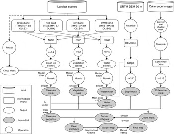
Fig. 2. Schematic workflow for mapping clean ice and debris-covered ice for the study area. Key steps in mapping clean ice include generation of clean-ice masks, masking of clouds and generation of water masks, while debris-covered glacier tongue mapping mainly consists of generating coherence maps and segmentation, producing vegetation and slope masks, overlay of all masks (coherence mask, slope mask, vegetation mask and clean-ice mask), neighborhood analysis and manual editing. The processing step ‘smooth’ represents spatial filtering of masks with open and close operations.
2.2. Landsat imagery
We obtained images acquired from the Landsat sensors including Landsat 8/OLI, Landsat 7/ETM+ and Landsat 5 TM, from the period, 2011 to 2013 (Table 1). Most of the images were acquired from Landsat 8, which started normal operations on 30 May 2013. Landsat 8/OLI provides images with more spectral bands and improved signal to noise radiometric performance compared with the previous Landsat sensors, enabling better characterization of land cover (U.S. Geological Survey, 2013). We inspected all the available scenes to select suitable images that are cloud-free over the glaciers and with minimum seasonal snow cover. However, it is almost impossible to get one image that is completely free from clouds in the summer season, due to frequent clouds and the prevalent orographic clouds. Meanwhile, there is a significant contrast in seasonal snow/ice coverage between warm and cold seasons. As a compromise between minimum seasonal snow cover and cloud cover, all available scenes acquired in August/September 2011–13 with low cloud coverage (at most 40%) were employed for glacier mapping in a schematic overlay frame (Section 3 below).
Table 1. List of Landsat satellite images and ALOS PALSAR scenes used in this study

For TM/ETM+ images, Bands 2, 3, 4, 5, 7 are used, while for OLI images, bands 3, 4, 5, 6, 7 are used.
All Landsat images used in this study were available from the United States Geological Survey (USGS) (http://earthexplorer.usgs.gov/). The images used are standard L1T products performed with systematic radiometric and geometric correction and in Universal Transverse Mercator (UTM) projection. Our study area belongs to UTM zone 46N and 47N and is covered by five scenes with different path/row combinations (Fig. 1; Table 1). For practical purpose, this study adopted UTM zone 46N as the projection for all mosaicked images and the final glacier inventory.
2.3. SAR scenes
For mapping debris-covered ice, we employ coherence images from SAR data. The coherence images are created from seven ALOS PALSAR image pairs (Section 3). The ALOS PALSAR sequential scenes were acquired from the ascending orbit in Fine-Beam Dual mode (FBD-HH/HV) with perpendicular baselines shorter than 410 m and a time interval of 46 or 92 d during the summer period of 2009 or 2010 (Fig. 1; Table 1). These PALSAR FBD data have an off-nadir angle of 34.3°, and the pixel spacing is ~5 m in the azimuth direction and 20 m in the range resolution. The L-band PALSAR data are preferred over the C- or X-band SAR data because the low-frequency system is less sensitive to decorrelation effects, so that changes in the surface properties can be easily shown in the coherence map (Atwood and others, Reference Atwood, Meyer and Arendt2010). In order to minimize the effect of spatial decorrelation, SAR image pairs with small baselines are preferred. The ALOS PALSAR data cover the majority of glacierized region (over 95%; Fig. 1).
2.4. DEM data
There are no available local or national DEMs of the study region with sufficient quality. However, two elevation datasets are available with near-global coverage, the DEM from the Shuttle Radar Topography Mission (SRTM) and the Advanced Spaceborne Thermal Emission and Reflection Radiometer (ASTER) Global DEM (GDEM), which are both accurate enough for compiling topographic glacier inventory data (Frey and Paul, Reference Frey and Paul2012). A subtraction of the ASTER GDEM from the SRTM DEM reveals differences of several hundred meters or up to 1 km in some regions. Visual examinations of hill shade views show some systematic shifts in the interpolated SRTM mask, indicating that the large bias is likely caused by erroneous interpolations in the SRTM data voids. This study replaced the erroneously interpolated values of SRTM3v4 with the corresponding ASTER GDEM (smoothed to reduce artificial bumps and holes and resampled to 90 m resolution before merging). The new SRTM DEM is void-free and smooth in hill shade view, and is used to compile the glacier inventory and to process the ALOS PALSAR coherence images. The percentage of the replaced data over the region is <1%, and mainly not within the glacierized region.
3. METHODOLOGY
Generation of the glacier inventory in SE QTP consists of three major steps: mapping clean ice with Landsat imagery, mapping debris-covered ice by combining Landsat, coherence images and DEM, and generation of ice divides and glacier parameters.
3.1. Mapping of clean ice
We employ a semi-automated method to generate a cloud-free mask by mosaicking several partly cloud-covered glacier masks. For clean ice mapping, the key steps include generation of glacier mask, cloud mask and open water surface mask from each Landsat scene (Fig. 2).
3.1.1. Preprocessing of Landsat scenes
We use normalized index images of different band combinations to highlight land information such as snow/ice, vegetation and water bodies. To derive normalized index images, calibration of Landsat scenes from raw digital numbers (DN) to Top-of-Atmosphere (TOA) reflectance is a first step and batch processed in ENVI/IDL platform. For Landsat8/OLI images, such calibration is done by referring to gain and offset parameters provided in the metadata files. For TM/ETM+ images, the calibration needs extra references to parameters such as mean exoatmospheric solar irradiance (ESUN) and earth/sun distance summarized by Chander and others (Reference Chander, Markham and Helder2009). TOA planetary reflectance is then derived by dividing TOA by the cosine of the sun elevation angle of the scene center. We use TOA planetary reflectance instead of DN, as it is preferable to work with data expressed in physical units and these calibrations may help standardize scenes from different dates and/or sensors (Burns and Nolin, Reference Burns and Nolin2014). The data gaps in the Landsat 7/ETM+ scenes due to failure of scan-line corrector are masked out with no-data filling value.
3.1.2. Generation of clean-ice masks
Clean-ice mask from individual Landsat scenes is generated by segmenting Normalized Difference Snow Index (NDSI) images. The NDSI is computed as the normalized difference between the reflectance of green band and short-wave infrared band (SWIR) (Landsat 8/OLI: (B3 − B6)/(B3 + B6); Landsat 7/ETM: (B2 − B5)/(B2 + B5)). The NDSI-based classification method is effective in removing some of the illumination differences on glaciers and yields satisfactory results for shaded ice (Racoviteanu and others, Reference Racoviteanu, Williams and Barry2008). Pixels with NDSI ≥ 0.4 and NDSI < 0.4 are, respectively, classified as potential clean-ice glaciers (value 1) and nonglaciers (value 255) in the mask, and when there are no data the value is set to 0. The threshold was developed based on experiments on glaciers sampled all over the world and has been proven effective (Hall and others, Reference Hall, Riggs and Salomonson1995). Mapping results are not sensitive to the changes of thresholds between 0.39 and 0.41.
3.1.3. Generation of cloud masks
As most of the Landsat scenes used are partly covered by cloud, a prerequisite step before mosaicking is to identify, which part of the images are contaminated by cloud. Such cloud-cover identification is implemented with the Fmask tool, which is available at https://code.google.com/p/fmask/. The latest Fmask tool, v3.2, is able to process Landsat 4, 5, 7 and 8 images (Zhu and others, Reference Zhu, Wang and Woodcock2015). This tool can generate cloud mask (with a value of 4) with high accuracy by applying a proper probability threshold (ranging from 0 to 100) in the input. We have tested a series of thresholds on different scenes and found that a threshold of 95–100 produced most accurate results for most scenes. The percentage of cloud area identified in a scene generally increases with the applied probability threshold, and stabilized after the threshold of 95. However, for several scenes that have low and thick cloud cover, such as the LE7/ETM+ image acquired on 23 August 2013, a high-probability threshold failed to identify the thick clouds distributed along the mountainsides. In such cases, a threshold of 50–60 can produce more satisfactory results. To maintain the highest percentage of clear pixels while identifying most cloud coverage, we recommend verifying the accuracy of cloud masks by superimposing them on corresponding Landsat false color composite images, such as Band 754 (RGB) for OLI images and Band 743 (RGB) for TM/ETM+.
3.1.4. Overlay and mosaic of clean-ice masks
The cloud mask generated by Fmask is used to mask the cloud-covered pixels by filling value 0 (no information) to the pixels, and then smoothed with a 3 × 3 kernel-size median filter to remove isolated pixels and fill small gaps. All individual masks are then mosaicked and overlaid into a single raster map within the maximum mosaic scheme. This scheme means that the non-glacier values (255) have a higher priority than glacier values (1) over overlapping areas. The lowest priority (0) denotes filling values and the cloud-covered pixels. The mosaic can retrieve minimum clean ice extent from multiple scenes and the cloud-covered pixels can be automatically removed and substituted by the clear pixels in other scenes. Figure 3a shows the original NDSI image, the single clean-ice mask by segmenting NDSI and the mosaic of all cloud-masked clean-ice masks, over a heavily glacierized subregion in the central study area (shown in Fig. 1). The example demonstrates that by overlying multi-temporal masks, glaciers under cloud-covered regions (highlighted in light grey in Fig. 3a(3)) in a single scene can be properly mapped from multi-temporal scenes.

Fig. 3. Selected key steps in generating clean-ice mask (a) and water mask (b). Column 1 is ratio images (NDSI/NDWI) of a single scene; column 2 gives the results of thresholding (binary image in black and dark grey) and then cloud masking (cloud in white); column 3 is the map of overlay and mosaic of all masks (with light grey indicating glaciers, which are obscured by clouds in a(2)); column 4 is the final results after spatial filtering (morphological open and close operations), with difference related to a(3) highlighted in light grey.
The mosaicked clean-ice mask needs to be smoothed to fill small holes and to remove small patches that originate from seasonal snow cover, mosaicking, cloud-detection and water-mask uncertainties. We apply morphological operators (open and close operation with disk structural element of 1-pixel radius) to smooth the final binary mask. The minimum size of glaciers to be included in the glacier inventory is set as 0.02 km2, equivalent to removal of small patches <23 pixels. The choice of the minimum glacier size depends on seasonal snow coverage and the resolution of the Landsat images, and consistency with other Landsat-based glacier inventories (Bajracharya and Shrestha, Reference Bajracharya and Shrestha2011; Frey and others, Reference Frey, Paul and Strozzi2012). Part of the smoothed clean-ice mask is shown in Figure 3a(4).
3.1.5. Generation, overlay and mosaic of water masks
It is worth noting that the smoothed clean-ice mask contains misclassifications caused by water bodies such as lakes, pro-glacial lakes and wide rivers, as they also show high-NDSI values. A common solution to this problem is to apply a threshold to the NIR band reflectance (TM/ETM band 4, OLI band 5) to eliminate water surfaces that are characterized by low reflection at the NIR band. This method, however, can eliminate shadowed or illuminated ice and humid glacier surfaces due to strong melting at the same time, resulting in fragmented patches in the classification maps.
We thus produce a water mask to remove water bodies, similar to the generation of a snow/ice mask. The method mainly includes four steps: (1) generation of ratio index image for each scene, (2) segmenting ratio images and masking clouds, (3) mosaicking and overlay of all scenes and (4) smoothing and post-processing. The Normalized Difference Water Index (NDWI) image is used as a main base for identifying water bodies. NDWI is computed as the normalized difference of the reflectance of green band and near infrared (NIR) band (TM/ETM+: (B2 − B4)/(B2 + B4); OLI: (B3 − B5)/(B3 + B5)) (McFeeters, Reference McFeeters1996). In the NDWI image, the unfrozen open water surfaces generally show high-NDWI values, in contrast to the slightly positive or negative NDWI shown by the non-water areas. A threshold of 0.15 is applied to segment the NDWI image into open water surface (value 1), non-water areas (255) and filling values (0). A major problem with the water masking is that shadowed areas are likely to be classified as water bodies. These misclassifications are removed by thresholding the mean slope of each water patch. If a polygon represents a real water surface, the mean slope should be very small. Referring to the bimodal distribution of mean slope of potential water polygons, a threshold of 15° is chosen to remove non-water polygons. This method is more effective than a pixel × pixel filtering of slope images, as the DEM is not up-to-date and some lakes may cover areas with large slopes due to expansion. During post processing, the polygons are dilated by two pixels, and then used to erase water surfaces from the clean-ice masks. The key steps in processing water masks are presented in Figure 3b.
3.2. Mapping of debris-covered glacier tongues
As an alternative to optical imagery, SAR data from active radar sensors are relatively independent of weather and solar illumination, and have been widely used to monitor surface deformations (e.g. Zhang and others, Reference Zhang2012; Hu and others, Reference Hu2014). One important estimate from SAR data is the coherence that shows the correlation between image pairs used in an interferometric operation. Since coherence is defined by phases and image intensities related to radar backscattering, the magnitude of coherence depends on many factors including sensor parameters (wavelength, polarization, system noise, slant range resolution), parameters related to the observation geometry (baseline, local incidence angle) and the surface properties (Atwood and others, Reference Atwood, Meyer and Arendt2010; Jiang and others, Reference Jiang, Ding, Hanssen, Malhotra and Chang2015). The influence of sensor- and geometry-dependent factors can be mitigated by appropriate interferometric processing. Volume decorrelation caused by penetration of the radar signal and temporal decorrelation caused by changes of target surface (i.e. motion and change of the scatterers) between image acquisitions are important to characterize properties of the observed surfaces. In particular, temporal decorrelation over glaciers can be severe in summer seasons, due to melting and freezing of ice and significant glacier flow that cause surface scattering and geometry changes. Thus low coherence can be used as a proxy for identifying glaciers (Atwood and others, Reference Atwood, Meyer and Arendt2010; Frey and others, Reference Frey, Paul and Strozzi2012).
One main problem with maps based on SAR data, including the coherence map, is the geometric distortions such as layover and shadow that can lead to data gaps over high-relief regions. Fortunately, the debris-covered glacier tongues, which are characterized by small slope angles, are in general free from the layover and shadow problems. Because other factors, such as melt of seasonal snow and growth of vegetation, can also lead to low coherence values, we combine multi-source data, including coherence image and additional information such as surface slope and land cover classifications (vegetation, glacier and water bodies) to map the debris-covered glacier tongues. The use of additional information is similar to the method proposed in Paul and others (Reference Paul, Huggel and Kääb2004). Specifically, the debris-covered parts are determined by six constraints: (1) coherence <0.15, (2) slope in the range 0°–25°, (3) not clean ice (value = 255 in the clean-ice mask, (4) not vegetation cover (value = 1 in the vegetation mask, introduced below), (5) not water bodies (value = 0 in the water mask) and (6) connection with clean ice. The processing is shown schematically in Figure 2 and described below.
3.2.1. Generation of coherence maps and segmentation
We use Gamma Remote Sensing interferometric tools (GAMMA) (Werner and others, Reference Werner, Wegmüller, Strozzi and Wiesmann2000) to derive single look complex (SLC) image pairs and interferometric coherence from the Level 1.0 ALOS PALSAR data. First, seven pairs of SLC images are derived by concatenating scenes along the track, range and azimuth compression, and by absolute radiometric calibration. The SLC image pairs are then co-registered with reference to topographic data. To remove the phase contribution from topography, a phase screen is simulated according to SRTM DEM and subtracted from the interferometric phase. In the interferometric processing, common band filtering and a multi-look of 6 × 14 in the range and azimuth direction are performed to reduce phase noises and reach approximately square pixels on the ground. An adaptive phase filter based on phase gradient (Goldstein and Werner, Reference Goldstein and Werner1998) is applied to maximize the coherence difference between the decorrelated and coherent areas, and an adaptive window size varying between 3 × 3 pixels and 9 × 9 pixels is used in coherence estimation. After terrain correction and geocoding, the final coherence images are in the UTM projection and at a spatial resolution of 30 m.
Glaciers and water bodies show very low coherence values (dark) in the resulting coherence images (Fig. 4a(1)). Areas affected by layover and shadow are identified with reference to the SAR imaging geometry and the topographic information (Fig. 4a(2); data gaps in white). To extract the low-coherence areas, a simple method is to apply a threshold on the coherence image. We determine the threshold empirically based on the distribution of coherence values over several large debris-covered glaciers that are manually delineated by referring to the false composite of Landsat images. The average coherence values over the tested glaciers range from 0.04 to 0.07, with standard deviations (σ) in the range 0.03–0.05. We determined a threshold of 0.15 (the averages of mean value ±2 σ) to extract potential debris-covered glacier parts.

Fig. 4. A subregion in the central area is selected to show the key steps in debris mapping. a(1): coherence image; a(2): coherence with data gaps masked out; a(3): resulting binary map of low-coherence areas (black) and others (data gaps and high-coherence areas in grey) after segmentation; a(4): final binary coherence mask after smoothing. b(1): NDVI image of a single scene; b(2): resulting map after thresholding and cloud masking (clouds in white, vegetation in grey and non-vegetation in black); b(3): mosaic of all vegetation masks; b(4): final binary vegetation mask after smoothing. c(1): false-color composite of Landsat 8 image; c(2): slope map of SRTM; c(3): resulting map after segmenting slope with a threshold of 25°, c(4): overlay of the binary coherence (a(4)), vegetation (b(4)), slope map(c(3)), clean ice (Fig. 3a(4)) and water (Fig. 3b(4)), showing clean ice in black, debris-covered ice in dark grey, water in light grey.
3.2.2. Generation of vegetation masks and slope mask
The vegetation masks are generated similarly to the water masks and clean-ice masks. The Normalized Difference Vegetation Index (NDVI), is used to segment the scenes into vegetation and non-vegetation areas. NDVI is computed as the normalized difference of the reflectance of NIR band and red band (TM/ETM: (B4 − B3)/(B4 + B3); OLI: (B5 − B4)/(B5 + B4)). NDVI can highlight the contrast between vegetation (high NDVI) and other land cover areas (low or negative NDVI values), and has been widely used to investigate vegetation cover (Tucker and others, Reference Tucker, Justice and Prince1986). Landsat images acquired in the summer seasons are suitable to define the maximum coverage of vegetation. We use a threshold of 0.2 to segment the scenes into vegetation-covered areas (NDVI > 0.2: value 255) and non-vegetation areas (NDSI < 0.2: value 1), according to the bimodal distribution of NDVI values in the scene. The vegetation mask derived from each scene is cloud masked, smoothed and then mosaicked to a single mask with the ‘maximum’ rule setting, which means retrieval of a maximum vegetation cover. The main steps in deriving the vegetation mask are shown in Figure 4b(1–4).
Thresholding on a slope image has proven to be an effective constraint in extracting areas with glacier tongue-like topography (Paul and others, Reference Paul, Huggel and Kääb2004; Veettil, Reference Veettil2012). Paul and others (Reference Paul, Huggel and Kääb2004) demonstrated that the slope of glacier tongues in a mountain glacier in the Swiss Alps does not exceed 24° in the case of complete coverage with debris. Similarly, this study applies a threshold of 25° to segment the slope map. The slope mask limits potential debris-covered areas to the relatively flat terrain.
3.2.3. Overlay of all masks and post processing
By overlaying the coherence mask, clean-ice mask, vegetation mask and slope mask, a binary mask defining the debris-covered ice is derived (Fig. 4c(4)). Smoothing of the mask is performed with a similar morphological operator to that introduced in Section 3.1. Generally debris-covered glaciers are connected with clean-ice parts. To remove isolated debris patches, we performed neighborhood analysis proposed by Paul and others (Reference Paul, Huggel and Kääb2004). The smoothed clean-ice mask and potential debris-cover mask are firstly transformed to vector formats, and then polygons connected with the clean ice are selected as the final debris-covered glacier parts.
The post processing step involves editing the clean-ice and debris-covered polygons to ensure seamless shared boundaries. The two kinds of polygons are then merged to form complete glacier outlines. Manual editing was also required for regions obscured by cloud cover in all images. In this case, we manually determined glacier outlines by referring to CGI2 and the PALSAR coherence map, which is helpful to reshape the glacier outlines. The separate mapping of clean-ice and debris-covered ice allows a straightforward distinction of the two types of glaciers and calculation of the percentage of debris cover for each glacier.
3.3. Delineation of ice divides
The last step in creating the glacier inventory is to separate individual glaciers along the hydrological divides. This step can affect the number and area of individual glaciers. To compile glacier drainage divides, we follow the automated approach described by Bolch and others (Reference Bolch, Menounos and Wheate2010) and derive hydrological basins by watershed analysis with the SRTM DEM clipped to a buffer of 1 km around the glacier outlines. The automatically derived drainage divides can contain errors due to inaccurate values in the DEM, particularly in the accumulation area and along the glacier margins (Fig. 5). The errors are inspected and manually improved with the help of the DEM in hill shade view, elevation contours and Landsat scenes. The individual glacier polygons are then derived by intersecting the original glacier polygons with drainage divides. Small polygons with area <0.02 km2 are omitted in the final glacier inventory. With reference to the DEM, glacier-specific parameters, including topographic information (minimum, maximum, mean and median elevation, mean slope and mean aspect in degree and mean aspect sector) are calculated for each glacier. In addition, an internal ID and the percentage of debris cover are assigned to each glacier.

Fig. 5. Comparison of basins derived from SRTM (red curves), ASTER (white curves) and manually corrected divides (yellow curves). Basins derived from SRTM and ASTER DEM show large discrepancies along the margins in the upper parts of some of the glaciers (black boxes in panel (a)). Many glaciers are already separated by ridges and do not need to be divided by drainage divides (black box in panel (b)) or can be easily isolated by one divide along the ridges (white box in panel (b)).
3.4. Creation of manual digitized outlines
Outlines of 55 glaciers (~170 km2) are manually digitized to test the accuracy of our mapping method. The digitization is based on Landsat imagery in a GIS and modified with reference to a slope map. We use the same ice divides to separate the glacierized area. The manually digitized outlines fall within different Landsat Path-Row combinations and cover clean-ice and debris-covered glaciers with a wide range of size classes (0.03–66 km2). Although a manually digitized dataset is considered highly precise, there is inherent error in any GIS-based manual digitization (e.g. Paul and others, Reference Paul2013) and determination of debris-covered glaciers is particularly difficult. We use surface features such as pro-glacial ponds and deposits in the glacier forefield as a sign of glacier termination when digitizing glacier outlines.
4. RESULTS
The 2013 glacier inventory of the SE QTP includes 6892 glaciers larger than 0.02 km2, covering a total area of 6566 km2. The distribution of the glaciers by number and by area per size class (Fig. 6a) and per mean aspect sector (Fig. 6b) shows typical patterns of mountain glaciers (e.g. Andreassen and others, Reference Andreassen, Paul, Kääb and Hausberg2008; Frey and others, Reference Frey, Paul and Strozzi2012). In this region, glaciers smaller than 1 km2 accounted for 84% of the total number, but they share only 20% of the total area. On the other hand, the 10 largest glaciers (>50 km2) cover ~13% of the glacierized area (853 km2). The mean elevation of different glaciers indicates that small glaciers (<1 km2) are distributed at higher elevations (99 m higher) than large glaciers. Analyzing the distribution of glaciers versus aspect sector reveals that with the SE–NW direction as a divide, the number and area of glaciers facing NE aspects (N, NE and E) notably exceeds those with SW aspects (S, SW and W) (Fig. 8b). About 56% of the total glacierized area has a northeast aspect. On the other hand, the mean elevation of glaciers with northeast aspects (5195 m) is 69 m lower than those with southwest aspects (5264 m).
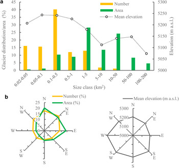
Fig. 6. Distribution of the number of glaciers (yellow), glacier area (green) and mean glacier elevations (circles), (a) per size class, (b) per aspect sector.
The spatial distribution of clean-ice and debris-covered ice is shown in Figure 7. About 8% (531.5 km2) of the glacierized area is covered by debris, with a mean elevation of 4337 m a.s.l. and mean slope of 12.1°. In contrast, the clean-ice glacier area (92% of total area) lies at higher elevations (5234 m a.s.l. on average) and on relatively rugged terrain with mean slope of 23.3°. A total of 338 glaciers have partly covered tongues, and these glaciers account for ~47% (3080 km2) of the total glacierized area. All glaciers >50 km2 and 84% of the glaciers >10 km2 have debris cover on their tongues, indicating large glaciers have a higher probability for debris cover on their tongues. The results from this study are consistent with previous observations that debris-covered glaciers tend to be the low-lying and low-slope tongues of large valley glaciers (Paul and others, Reference Paul, Huggel and Kääb2004; Frey and others, Reference Frey, Paul and Strozzi2012). The hypsometry of all analyzed glaciers in the study region is shown in Figure 8. While almost 92% of the total glacierized area is debris free, the amount of debris-covered ice is more dominant in areas below 4100 m.

Fig. 7. Spatial distribution of inventoried glaciers (including the debris-covered parts and clean-ice parts) and data gaps where images are always cloud covered.

Fig. 8. Hypsometry of glacierized region in the study area, with elevation varying in the range 2522–7203 m.
Mean elevation is often used as a good approximation for the ELA and thus is a suitable parameter to analyze the governing climatic conditions. Figure 9 shows the distribution of mean elevation of individual glaciers. For clarity, only glaciers >1 km2 are shown. The spatial distribution of glacier mean elevations reflects such climate dependence in the SE QTP. Following the Yarlung Tsangpo great canyon from south to north, the Indian summer monsoon brings moisture inward, which results in a relatively maritime climate on the southern slope and eastern facets of the mountain ranges, and the lowest mean elevation of glaciers (below 4500 m) around the Great Bend of Yarlung Tsangpo (Fig. 9). From there, the mean elevation increases in SE–NW and SW–NE directions (indicated by white arrows in Fig. 9), with the highest mean elevations (above 5500 m a.s.l.) in the northwestern and southeastern margins of the study region. The two gradients reflect change in the climate conditions associated with both the extension of large canyons, which serve as an important moisture transportation path, and high-mountain ranges, which block water vapor to the leeward side and inner highlands. It is interesting to note that with the pattern of variability in mean glacier elevation, the debris coverage decreases from ~28% in the SE (mean elevation <4500 m a.s.l.) to only 3% in the NW (mean elevation > 5500 m a.s.l.) (Fig. 9). This phenomenon is similar to that found over the Bhutan Himalaya (Kääb, Reference Kääb2005) and the western Himalayas (Frey and others, Reference Frey, Paul and Strozzi2012). The suggested possible explanations, intensive debris supply from the steep rock walls in the south, different geology from the southern edges of plateau to the inner area, and auto-correlation effects between debris cover and low-elevation glacier parts, may also apply here.

Fig. 9. Outlines of all inventoried glaciers in this study and mean elevation of individual glaciers with size >1 km2 (represented by color-filled circles). The Great Bend of Yarlung Tsangpo region has the most humid climate and the mean elevation increases in both the NW and SE directions (indicated by the white dashed curves). The debris coverage (indicated by the number in brackets in the legend) decreases with increasing elevation.
The water vapor transportation paths along with the topographic variations result in regional differences in glacier distributions. The study region can be divided into six subregions, roughly along the major canyons, which act as natural divides of different mountain ranges and climate patterns (Fig. 9). Table 2 gives a summary of some selected glacier parameters for each subregion. Sub-region A in the NW represents the high-inner plateau, where the climate is relatively dry and cold and is less influenced by the monsoons. Glaciers in these regions are characterized by high elevation, low debris cover and small area (mean area < 0.5 km2). Sub-regions C, D and F in the south and east have a relatively maritime climate due to influences from the summer monsoon, resulting in lower mean elevation, higher percentage of debris cover and large glacier area (dominated by size class between 10 and 50 km2). Glaciers in sub-region D have the highest rate of debris cover (16.3%). About 48, 22 and 12% of the total debris-covered area are distributed in sub-region C, F and D, respectively. It is interesting to note that the glaciers in sub-region F in the southern bank of Parlung Tsangpo have the lowest mean elevation (<5000 m), 400 m lower on average than those in sub-region E in the northern bank, which reflects the maritime (dry) climate in the southern (northern) side of the mountain ranges. Sub-region B represents a medium state between the maritime SE (sub-region D and C) and the dry NW (sub-region A).
Table 2. Glacier parameters for each subregion of the SE QTP

5. DISCUSSION
5.1. Glacier inventory data and accuracy
The manually digitized glacier outlines (as control dataset) are distributed over four heavily glacierized subregions (Fig. 10). There is good agreement between our glacier inventory and the control dataset, despite that the former exhibits noise edges (Fig. 10). The 55 control glaciers have a total area of 176.3 km2 in the control dataset, compared with 171.4 km2 in our generated glacier inventory. This is equal to an overall −2.9% percentage difference (total areal difference divided by the total glacier area). The 30 median-to-large glaciers (>0.2 km2), covering 95% of total area, show stable extents in the two datasets, with areal percentage difference varying between −7 and 3% (−2.5% on average); while 10 smallest glaciers (<0.1 km2) tend to be 10% smaller on average in our generated glacier inventory than in the control dataset. This is reasonable as our retrieved outlines represent conserved glacier extents by mapping minimal area with multi-temporal Landsat scenes, whereas the manual digitized dataset is referred to a single Landsat scene. This effect can be particularly obvious for small glaciers, which tend to show fast temporal variations (Dyurgerov and Meier, Reference Dyurgerov and Meier2000). Although the number of digitized glaciers may be not enough, we consider the validation as roughly representative and estimate an uncertainty of 3% for the total mapped glacier area (6566 km2).
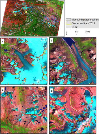
Fig. 10. The 2013 glacier inventory generated in this study (yellow) compared with a couple of manually digitized glacier outlines (black) and the second CGI (CGI2). Overall there is good coherence between the 2013 glacier inventory and the manual dataset. The CGI2 shows inconsistent qualities across the study region, with overestimation in the heavily glacierized central area (e.g. (a) and (b)), acceptable quality in the northeastern area (e.g. (c)) and problematic inner glacier boundaries in the southeastern area (e.g. (d)).
The total number of mapped glaciers (6892) depends on the minimum size threshold (here, 0.02 km2). If this value is set to 0.05 km2, the number reduces to 5783, covering a total area of 6529 km2. In the CGI2, the total number of glaciers >0.05 km2 is 6122 and the total area is 9744.6 km2. The considerable difference in the glacier area (>3000 km2) may partly be explained by glacier changes (retreat). However, it is more likely that the glacierized area in the CGI2 was overestimated due to errors such as misclassification of proglacial lakes, seasonal snow cover and inaccurate inner ice boundaries (Fig. 10). The quality of CGI2 is inconsistent across the study area, with remarkable overestimation in the heavily glacierized region in the central and southeastern part, yet acceptable quality in the northeastern part (Fig. 10). We speculate that the inconsistent quality is probably associated with different qualities of reference data for updating CGI2, despite that it is unclear, which images were used for different parts.
Under cloud-free conditions, automated clean ice mapping methods may have an uncertainty of ±1 pixel (30 m) in an outline position, as shown in previous research (e.g. Paul and others, Reference Paul, Huggel, Kääb, Kellenberger and Maisch2002; Andreassen and others, Reference Andreassen, Paul, Kääb and Hausberg2008). The main uncertainties of our method lie in the use of partly cloud-covered images, which demands high accuracy of cloud mask generation and geometric accuracy of the images. Failure in identifying clouds over a glacierized area may lead to erroneous classification of glaciers. We recommend checking the accuracy of the produced cloud mask and dilating it with 1–3 pixels to ensure complete mask out of a cloud-affected region. The Landsat 1T products, particularly the Landsat 8 scenes, have a high-geometric accuracy within 13 m (less than on-pixel resolution) (Storey and others, Reference Storey, Choate and Lee2014), which ensures reliable overlay of multiple scenes. Note that data gaps may still exist due to persistent orographic cloud cover (Fig. 7). However, the always cloud-covered areas only account for a small percentage of the total study area (6%), and they are not heavily glacierized, with total glacier area ~77 km2 (1.2% of the total glacierized area).
The accuracy of the DEM affects the glacier inventory, mainly in two ways: the generation of glacier divides and the derived topographic parameters of glaciers. There may be local shifts between the Landsat imagery and SRTM, as revealed by the differences between drainage divides derived from SRTM and interpreted from Landsat imagery (Fig. 5). The uncertainties in the glacier divides, however, have no impact on the total mapped glacier area.
5.2. Semi-automated mapping of debris-covered ice with coherence
Due to the presence of data voids in the coherence images over rugged mountainous areas, automated glacier mapping based solely on SAR data is difficult. This study demonstrates the potential of semi-automated mapping of debris-covered glacier tongues that have low slopes and are almost free from data voids in the coherence images. A threshold of 0.1–0.15 on the coherence image and overlay of multi-source data are straightforward and efficient for extracting potential debris-covered glacier tongues. It is worth noting that manual interpretation of debris-covered parts based solely on slope information and Landsat images can be misleading, as there are many glacier-tongue shapes, which turn out to be nonglaciers (Fig. 11). This shows the necessity of employing coherence information in debris-covered ice mapping. With constraint of low coherence and gentle slope, potential rock glaciers and non-moving dead ice are not included in this glacier inventory. To map these glaciers, a combined analysis with coherence, time series and high-resolution data need to be conducted.
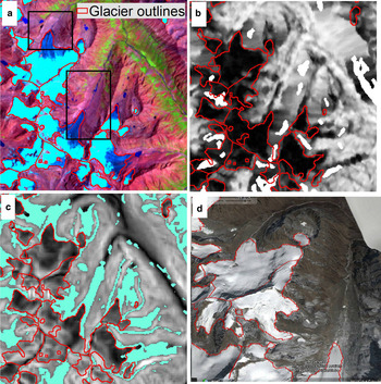
Fig. 11. An illustration of challenging conditions for identifying debris-covered ice over the SE QTP. Some areas (black rectangle in (a)) with glacier tongue-like topography and connected with a clean-ice glacier turns out not to be debris-covered glacier, as (b) shows relatively high-coherence values compared with the surrounding non-glacier region. The shaded green areas in (c) highlight tongue-like topography determined by overlaying non-clean-ice, low slope, non-water and non-vegetation masks. (d) Close-up detail about the black rectangle area based on high-resolution images (acquired on 8 November 2014) from Google Earth.
6. CONCLUSIONS
With a combination of multi-source information from the latest Landsat observations, SRTM DEM and SAR data, this study presents a semi-automated approach for generating a glacier inventory for the SE QTP under challenging mapping conditions (significant terrain relief, debris cover and serious effects from clouds). To reduce the influences of cloud cover, the use of multi-temporal Landsat observations was suggested in previous glacier inventory mapping; however the method for doing this usually involves manual editing and is time- and labor- consuming for a large region. We propose a semi-automated scheme to combine the multi-temporal and multi-source data, based on simple rules of data selection and processing. Most thresholds used for map segmentations are based on distribution of image values (e.g. NDSI, NDVI and NDWI) and most processing steps are semi-automated and pixel-based, significantly reducing the requirement of manual editing and improving the accuracy of glacier mapping. To map debris-covered glacier tongues, we extended the multi-source method proposed by Paul and others (Reference Paul, Huggel and Kääb2004) by adding coherence images from SAR data. Including such information is essential and necessary as many glacier-tongue shapes turn out to be nonglaciers in this region. The proposed method can potentially be used for glacier mapping in similar regions including the Himalaya.
The new glacier inventory for the SE QTP is the most comprehensive to date for the region. The study has also revealed that the glacierized area in CGI2 was significantly overestimated (>30%) probably due to the use of cloud-free images that may contain large seasonal snow cover. The new glacier inventory identifies 6892 glaciers >0.02 km2, covering a total area of 6566 ± 197 km2 (3% uncertainty). The debris-covered glacierized areas account for ~8% of the total area (532 km2), and they are restricted to lower elevations (mostly below 4600 m) with moderate terrain gradients. From the eastern and southern end of the Nyainqentanglha ranges to the inner plateau in the NW, there is an increase in the mean glacier elevation of 2000 m and a general decreasing trend of debris coverage, reflecting different climatic, topographic and geological conditions. We have classified the region into six subregions, roughly along the major canyons that act as natural divides of the different mountain ranges and climate conditions. The new glacier inventory will benefit future glacier studies including assessment and modeling of glacier changes and the impacts on runoff, projecting glacier developments and glacier lake hazards.
ACKNOWLEDGEMENTS
Landsat images were obtained from the U.S. Geological Survey. PALSAR data were provided by Japan Aerospace Exploration Agency (JAXA) through project P1246002. SRTM DEM image was derived from the Consultative Group for International Agricultural Research. The first author is grateful for the Ph.D. studentship offered by the Hong Kong Polytechnic University. The research was supported by the Research Grant Council (RGC) of Hong Kong Special Administrative Region (Grant Numbers: PolyU5146/11E and PolyU 5147/13E), by NASA (No. NNX13AQ89G), NSFC (No. 41374020) and State Key Laboratory of Geodesy and Earth's Dynamics, Institute of Geodesy & Geophysics, Chinese Academy of Sciences (No. Y309473047). We sincerely thank two reviewers (B. Raup and F. Paul) for their helpful feedback and constructive suggestions.


 Open access