


1. Introduction
Chemically active particles can undergo self-diffusiophoresis in liquid solutions by engendering concentration gradients through chemical reactions (Paxton et al. Reference Paxton, Kistler, Olmeda, Sen, Angelo, Cao, Mallouk, Lammert and Crespi2004; Moran & Posner Reference Moran and Posner2017). In their influential work, Golestanian, Liverpool & Ajdari (Reference Golestanian, Liverpool and Ajdari2007) proposed the first macroscale model for self-diffusiophoresis. It assumes Stokes flow conditions and diffusive transport of solute. On the particle boundary, chemical reactions are represented by a prescribed distribution of solute flux; mechanical interactions with solute molecules are assumed to occur within a thin boundary layer relative to the particle size, hence modelled by an effective diffusio-osmotic slip (Anderson Reference Anderson1989). Due to the linearity of the governing equations and boundary conditions, self-propulsion is predicted only for particles exhibiting asymmetry in their shapes or physicochemical properties.
A nonlinear extension of that model, incorporating advective transport of solute, was later proposed by Michelin, Lauga & Bartolo (Reference Michelin, Lauga and Bartolo2013). The extended model predicts that a spherical particle with homogeneous physicochemical properties can self-propel via a symmetry-breaking mechanism. Two necessary conditions are: (i) the particle activity and slip coefficient must have the same sign; and (ii) the intrinsic Péclet number  $Pe$, indicating the strength of advection relative to diffusion, must be greater than $4$. While particles typically do not satisfy the latter condition (Moran & Posner Reference Moran and Posner2017), active droplets were observed experimentally to move spontaneously as a result of an analogous symmetry-breaking mechanism (Izri et al. Reference Izri, Van Der Linden, Michelin and Dauchot2014).
The macroscale description of Michelin et al. (Reference Michelin, Lauga and Bartolo2013) has since served as the basis for multiple subsequent analyses of both asymmetry-driven (Michelin & Lauga Reference Michelin and Lauga2014; Yariv Reference Yariv2016, Reference Yariv2017; Yariv & Kaynan Reference Yariv and Kaynan2017) and spontaneous (Desai & Michelin Reference Desai and Michelin2021, Reference Desai and Michelin2022; Saha, Yariv & Schnitzer Reference Saha, Yariv and Schnitzer2021; Picella & Michelin Reference Picella and Michelin2022; Peng & Schnitzer Reference Peng and Schnitzer2023; Schnitzer Reference Schnitzer2023) motion, and has also been adopted as a reference model for active droplets (Michelin Reference Michelin2023). In particular, several recent extensions of Michelin et al. (Reference Michelin, Lauga and Bartolo2013) have investigated the dynamics of isotropically active spheres constrained by solid boundaries (Yariv Reference Yariv2016, Reference Yariv2017; Desai & Michelin Reference Desai and Michelin2021, Reference Desai and Michelin2022; Picella & Michelin Reference Picella and Michelin2022). In purely hydrodynamic settings, the presence of boundaries leads naturally to increased viscous resistance to particle motion (Happel & Brenner Reference Happel and Brenner1965). Nonetheless, it has been shown that confinement promotes the spontaneous motion of active particles, leading to symmetry breaking at smaller  $Pe$ (Desai & Michelin Reference Desai and Michelin2021, Reference Desai and Michelin2022).
In a recent study, Picella & Michelin (Reference Picella and Michelin2022) presented a particularly dramatic effect of confinement on the spontaneous motion of active particles. Those authors performed time-dependent simulations of an active spherical particle moving through a cylindrical channel, the latter being represented by a large but finite computational domain truncated at two remote cross-sections. (See §§ 3 and 4 of that paper for a detailed description of the numerical method employed.) In a frame of reference moving with the particle, reportedly the simulated system reaches a stable steady state where the centre of the particle is aligned with the channel axis; the geometry of this axisymmetric configuration can be characterised by  $\epsilon$, the ratio of the minimum particle–channel clearance to the particle radius. Focusing on axisymmetric steady states, Picella & Michelin (Reference Picella and Michelin2022) reported a bifurcation from a stationary symmetric state when $Pe$ exceeds a critical threshold. The reported critical $Pe$ is a function of $\epsilon$, say $Pe_c(\epsilon )$, that decreases rapidly with decreasing $\epsilon$ ( $Pe_c\approx 4$ for large $\epsilon$, and $Pe_c\approx 0.1$ for $\epsilon \approx 1$). Unfortunately, Picella & Michelin (Reference Picella and Michelin2022) could not investigate closely fitting particles ( $\epsilon \ll 1$) as their numerical method is not accurate for small $\epsilon$; in fact, they could not determine $Pe_c$ accurately even for moderately small $\epsilon$ ( $\epsilon \lesssim 1$).
Picella & Michelin (Reference Picella and Michelin2022) supplemented their simulations with analytical arguments, including a steady-state integral solute balance ((5.3) therein) in a reference frame moving with the particle, assuming an infinitely long channel. We draw attention to two direct consequences of that balance. First, the problem is ill-posed for  $Pe = 0$, indicating that the small- $Pe$ limit is singular. Second, any solution for $Pe>0$ must involve particle motion at a non-zero speed relative to the channel walls, accompanied by a fore–aft asymmetric solute concentration. Consequently, there cannot be a bifurcation at finite $Pe$ from a symmetric solution with a stationary particle to an asymmetric solution involving spontaneous motion. This latter conclusion, seemingly overlooked by Picella & Michelin (Reference Picella and Michelin2022), reveals that the reported bifurcations and the calculated values of $Pe_c$ can be interpreted only as numerical artefacts.
Despite the above difficulties in the interpretation of the numerical results in Picella & Michelin (Reference Picella and Michelin2022), their model – which is a direct extension of that in Michelin et al. (Reference Michelin, Lauga and Bartolo2013) – provides a useful starting point for the analysis of confined active particles. Moreover, their simulations suggest that achieving spontaneous motion at small values of  $Pe$, which is representative of typical active particles, is possible under confinement. Accordingly, a systematic investigation of the spontaneous motion of confined active particles at small $Pe$ could pave the way for experimental demonstrations of this phenomenon in particles.
Accordingly, the present paper aims to analyse the motion of an isotropically active particle at small Péclet numbers ( $Pe\ll 1$). As in Picella & Michelin (Reference Picella and Michelin2022), we will adopt the macroscale description of Michelin et al. (Reference Michelin, Lauga and Bartolo2013). We will focus on closely fitting particles ( $\epsilon \ll 1$), corresponding to a regime where a detailed asymptotic description of the problem can be constructed systematically following the method of matched asymptotic expansions (Hinch Reference Hinch1991) – as in classical studies of moving particles closely fitting in channels (see e.g. Bungay & Brenner Reference Bungay and Brenner1973). We note that this regime has not been considered by Picella & Michelin (Reference Picella and Michelin2022) due to the aforementioned limitations of their numerical method.
The paper is structured as follows. We describe the physical problem in § 2, and formulate the mathematical problem in § 3. In § 4, we derive integral balances for the mass and solute concentration. In § 5, we perform a scaling analysis in the small- $\epsilon$ and small- $Pe$ regime, which will allow us to determine the appropriate distinguished limit for the problem. In § 6, we perform an asymptotic analysis of the problem in this distinguished limit. We discuss our results in § 7.
2. Physical problem
Consider a chemically active spherical particle (radius  $a^*$) moving within a cylindrical channel (radius $b^*>a^*$) filled with an otherwise quiescent fluid (viscosity $\mu ^*$) that contains a single species of solute molecules (diffusivity $D^*$).
The particle exchanges solute with the fluid at a uniform rate per unit area  $A^*$. This activity generates variations in the solute concentration, which are transported across the channel via advection and diffusion. Concurrently, changes in the concentration along the particle surface induce an effective diffusio-osmotic slip directly proportional to the surface gradient of the concentration. The proportionality constant, namely the slip coefficient $M^*$, is also assumed uniform.
We will henceforth look for axisymmetric solutions of the problem where the particle moves along the channel axis at a constant speed. (We note that in the time-dependent simulations of Picella & Michelin (Reference Picella and Michelin2022), those axisymmetric solutions were found to be stable attractors for the problem.) Since the physicochemical properties of the spherical particle are homogeneous, the problem lacks a preferred direction along the channel axis. As demonstrated in previous works (Michelin et al. Reference Michelin, Lauga and Bartolo2013; Picella & Michelin Reference Picella and Michelin2022), the symmetry breaking leading to spontaneous motion can occur only if  $M^*$ and $A^*$ have the same sign. Motivated by that, we will assume $M^* A^*>0$.
If the particle indeed exhibits symmetry-breaking spontaneous motion, then dimensional arguments show that (Golestanian et al. Reference Golestanian, Liverpool and Ajdari2007)
 \begin{equation} \text{particle speed} = \mathcal{W}\times \frac{M^*A^*}{D^*}. \end{equation}
Here,  $\mathcal {W}$ is the dimensionless speed, which depends upon two strictly positive parameters, namely the dimensionless clearance,
 \begin{equation} \epsilon = \frac{b^*-a^*}{a^*}, \end{equation}
and the intrinsic Péclet number,
 \begin{equation} Pe = \frac{M^*A^ *a^*}{D^{*2}}. \end{equation}
It is convenient to discuss solute transport in the co-moving reference frame, where the flow and concentration fields are steady. Far upstream, corresponding to the direction of the particle motion in the laboratory frame, the solute concentration approaches a uniform value, which by causality must be independent of the particle's activity; far downstream, the concentration saturates at a different uniform value due to the accumulation of solute generated by the particle and advected by the flow. Dimensional arguments show that, relative to its value far upstream,
 \begin{equation} \text{solute concentration far downstream} = \mathcal{C}^-\times \frac{A^* a^*}{D^*}. \end{equation}
Just like  $\mathcal {W}$, the dimensionless downstream concentration $\mathcal {C}^-$ depends upon $\epsilon$ and $Pe$.
$Pe$.
3. Dimensionless formulation
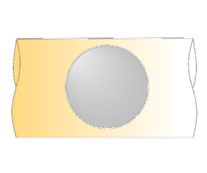
We proceed to formulate the dimensionless steady-state problem in the co-moving reference frame, as illustrated in figure 1(a).

Figure 1. Schematic diagrams depicting (a) the dimensionless problem in the co-moving reference frame and (b) the geometry of the gap region.
We normalise lengths by  $a^*$ and introduce the cylindrical coordinates $(r,\phi,z)$ with the origin at the centre of the particle; $r$ measures the radial distance from the channel axis, $\phi$ is the azimuthal angle, and the $z$-axis coincides with the channel axis and points in the direction of the particle's motion relative to the channel. The surface of the particle, denoted by $\mathcal {S}$, is parametrised as $r = f(z)$ with
 \begin{equation} f(z) = \sqrt{1 - z^2}\quad\text{for }|z|\leq 1, \end{equation}
and the channel wall is located at  $r = 1 + \epsilon$. The fluid domain, denoted by $\mathcal {F}$, is given by $f(z) < r < 1 + \epsilon$ for $|z|\leq 1$, and $r < 1 + \epsilon$ for $|z|> 1$.
We denote the excess solute concentration (normalised by  $A^* a^*/D^*$), relative to its upstream value, by $c$ (if $A^*<0$, then $c$ represents a concentration deficit), the pressure (normalised by $\mu ^*M^*A^*/a^*D^*$) by $p$, and the velocity (normalised by $M^*A^*/D^*$) by $\boldsymbol {u}$. Axial symmetry dictates that the flow and concentration fields are independent of $\phi$ and that the velocity field can be written as
 \begin{equation} \boldsymbol{u} = u\hat{\boldsymbol{r}} + w\hat{\boldsymbol{z}}, \end{equation}
where  $\hat {\boldsymbol {r}}$ and $\hat {\boldsymbol {z}}$ are unit vectors associated with the $r$ and $z$ coordinates, respectively.
The flow is governed by the Stokes equations
 \begin{equation} \boldsymbol{\nabla} p = \nabla^2 \boldsymbol{u},\quad \boldsymbol{\nabla}\boldsymbol{\cdot} \boldsymbol{u} =0\quad \text{in } \mathcal{F}, \end{equation}
the diffusio-osmotic slip condition (Anderson Reference Anderson1989; Golestanian et al. Reference Golestanian, Liverpool and Ajdari2007)
 \begin{equation} \boldsymbol{u} = \boldsymbol{\nabla}_s c\quad \text{on } \mathcal{S}, \end{equation}
wherein  $\boldsymbol {\nabla }_s = (\mathsf {I} -\hat {\boldsymbol {n}}\hat {\boldsymbol {n}})\boldsymbol {\cdot } \boldsymbol {\nabla }$, with $\mathsf {I}$ being the idemfactor and $\hat {\boldsymbol {n}}$ the outward unit normal (note that $\hat {\boldsymbol {n}}\boldsymbol {\cdot } \boldsymbol {u}=0$), the no-slip condition
 \begin{equation} \boldsymbol{u} ={-}\mathcal{W}\hat{\boldsymbol{z}}\quad \text{at } r = 1+\epsilon, \end{equation}
the far-field condition, specifying that the fluid is quiescent far from the particle in the laboratory frame,
 \begin{equation} \boldsymbol{u} \to -\mathcal{W}\hat{\boldsymbol{z}}\quad \text{as } z\to\pm\infty, \end{equation}
and the force-free condition
 \begin{equation} \int_{\mathcal{S}} \hat{\boldsymbol{n}} \boldsymbol{\cdot} [{-}p\mathsf{I} + (\boldsymbol{\nabla}\boldsymbol{u}) + (\boldsymbol{\nabla}\boldsymbol{u})^{\dagger}]\boldsymbol{\cdot} \hat{\boldsymbol{z}}\, \text{d} S =0, \end{equation}
with  ${\dagger}$ denoting the tensor transpose, and $\text {d} S$ denoting a differential area element.
The concentration field satisfies the advection–diffusion equation
 \begin{equation} Pe \,\boldsymbol{u}\boldsymbol{\cdot} \boldsymbol{\nabla} c =\nabla^{2} c\quad \text{in } \mathcal{F}, \end{equation}
subject to the activity condition
 \begin{equation} \hat{\boldsymbol{n}}\boldsymbol{\cdot} \boldsymbol{\nabla} c ={-}1\quad\text{on } \mathcal{S}, \end{equation}
the no-flux condition
 \begin{equation} \hat{\boldsymbol{n}}\boldsymbol{\cdot} \boldsymbol{\nabla} c = 0\quad\text{at } r =1 + \epsilon, \end{equation}
and the upstream and downstream conditions, respectively,
 \begin{equation} c\to 0 \text{ as } z\to\infty,\quad c\to \mathcal{C}^{-}\text{ as } z\to-\infty. \end{equation}
4. Integral balances
We now derive exact integral balances that will facilitate our analysis.
To begin, we integrate the advection–diffusion equation (3.8) over the entire fluid domain and apply the divergence theorem together with (3.3b)–(3.6) and (3.9)–(3.11a,b). This furnishes the relation
 \begin{equation} Pe\, \mathcal{W}\mathcal{C}^-(1 + \epsilon)^2 = 4, \end{equation}
which has been derived previously by Picella & Michelin (Reference Picella and Michelin2022) – see (5.3) therein. This relation represents a balance between the net advective flux far downstream and the activity (3.9) integrated over the particle surface; in particular, it allows us to determine  $\mathcal {C}^-$ once $\mathcal {W}$ is known. Clearly, (4.1) implies that the problem is ill-posed for $Pe=0$ and that stationary solutions ( $\mathcal {W}=0$) are impossible.
Next, we derive cross-sectional balances describing conservation of mass and solute between a cross-section of the channel located far upstream ( $z\to \infty$) and another cross-section located arbitrarily ( $z = \mathcal {Z}$) in the gap between the particle and the channel wall ( $|\mathcal {Z}|\leq 1$). To obtain the cross-sectional mass balance, we integrate the continuity equation (3.3b) over the domain $\mathcal {F}_\mathcal {Z} = \{(r,z)\in \mathcal {F}\, | \,z\geq \mathcal {Z}\}$ and apply the divergence theorem in conjunction with (3.4)–(3.6). This yields
 \begin{equation} \int_{f(\mathcal{Z})}^{1 + \epsilon}w|_{z=\mathcal{Z}}r \, \text{d} r ={-}\tfrac{1}{2}\mathcal{W}(1 + \epsilon)^2. \end{equation}
(Note that the slip velocity (3.4) has zero normal component and hence does not contribute to the mass balance.)
To obtain the cross-sectional solute balance, we integrate (3.8) over  $\mathcal {F}_\mathcal {Z}$ and apply the divergence theorem in conjunction with (3.3b)–(3.6) and (3.9)–(3.11a,b). This yields
 \begin{equation} \int_{f(\mathcal{Z})}^{1 + \epsilon} \left.\left(Pe \,w c - \frac{\partial c}{\partial z} \right)\right|_{z=\mathcal{Z}} r \, \text{d} r ={-}1 + \mathcal{Z}. \end{equation}
The right-hand side represents the integration of the activity (3.9) over the spherical cap  $\mathcal {S}\cap \partial \mathcal {F}_\mathcal {Z}$.
5. Closely fitting particle: scalings
We focus hereafter upon the narrow gap and small Péclet number regime,  $\epsilon \ll 1$ and ${Pe\ll 1}$. We begin with a scaling analysis. In addition to providing insight into the problem, our scalings will allow us to determine the appropriate distinguished limit for the subsequent asymptotic analysis.
Let us first describe the local geometry of the gap between the particle and channel, illustrated in figure 1(b). There, the surface of the particle is approximately paraboloidal, and the particle–channel separation  $h(z) =1 + \epsilon - f(z)$ can be expanded as
 \begin{equation} h(z)=\epsilon + \tfrac{1}{2}z^2 + \cdots\quad \text{as } z\searrow0. \end{equation}
Examining the first two terms of this expansion, we see that the separation remains of order  $\epsilon$ over axial distances of order $\epsilon ^{1/2}$. We postulate that the characteristic radial and axial length scales in the vicinity of the gap are given by $\epsilon$ and $\epsilon ^{1/2}$, respectively.
Regarding the flow in the gap, the cross-sectional mass balance (4.2) implies that the axial velocity in the far field, of order  $\mathcal {W}$, is amplified by a factor $\epsilon ^{-1}$ as the narrow gap is approached. Therefore, the axial velocity in the gap scales as $\mathcal {W}/\epsilon$. The continuity equation (3.3b) suggests that the radial velocity in the gap scales as $\mathcal {W}/\epsilon ^{1/2}$; the axial component of the momentum equation (3.3a) suggests that the pressure in the gap scales as $\mathcal {W}/\epsilon ^{5/2}$; and the diffusio-osmotic slip condition (3.4) suggests that the solute concentration scales as $\mathcal {W}/\epsilon ^{1/2}$.
Given the above, we now consider solute transport in the gap. With the advective flux  $Pe\,wc$ scaling as $Pe\, \mathcal {W}^2/\epsilon ^{3/2}$, and the diffusive flux $-\partial c/\partial z$ scaling as $\mathcal {W}/\epsilon$, the cross-sectional solute balance (4.3) leads to the scaling relation
 \begin{equation} \left(\frac{Pe\, \mathcal{W}^2}{\epsilon^{3/2}}+\frac{\mathcal{W}}{\epsilon} \right)\times \epsilon \sim 1. \end{equation}
This relation indicates that  $\mathcal {W}$ is of order unity for $Pe$ at most of order $\epsilon ^{1/2}$, and is asymptotically small for $Pe\gg \epsilon ^{1/2}$. (Curiously, our scalings also suggest that order-unity speeds could be possible at small $Pe$ even for $\epsilon$ of order unity. We return to this point in § 7.)
Balancing the three terms appearing in (5.2), the appropriate distinguished limit to be considered in the subsequent asymptotic analysis is
 \begin{equation} Pe= O(\epsilon^{1/2}), \end{equation}
with the particle speed being
 \begin{equation} \mathcal{W}= O(1). \end{equation}
Moreover, in this distinguished limit, (4.1) implies that
 \begin{equation} \mathcal{C}^-= O(\epsilon^{{-}1/2}). \end{equation}
Importantly, our scaling arguments suggest that (5.3) is the only distinguished limit in the regime where  $\epsilon$ and $Pe$ are small, as it corresponds to a general scenario where advection and diffusion are accounted for in the gap region
6. Closely fitting particle: asymptotic analysis
We now analyse the distinguished limit (5.3), represented by
 \begin{equation} \epsilon\ll1,\quad Pe= \epsilon^{1/2}\,\overline{Pe}, \end{equation}
with  $\overline {Pe}$ held fixed. In view of (5.4) and (5.5), we pose the expansions
 \begin{equation} \mathcal{W} = \mathcal{W}_{0} + \cdots,\quad\mathcal{C}^-= \epsilon^{{-}1/2} \mathcal{C}^-_{{-}1/2} + \cdots, \end{equation}
where the leading-order balance of (4.1) reads
 \begin{equation} \overline{Pe}\,\mathcal{W}_0\,\mathcal{C}^-_{{-}1/2} = 4. \end{equation}
6.1. Remote regions
We commence our asymptotic analysis by examining the flow and solute transport in the upstream ( $z>0$) and downstream ( $z<0$) remote regions of the channel. In those regions, advection and diffusion balance (3.8) over a (dimensionless) length scale of order $(Pe\,\mathcal {W})^{-1}$, which, by (5.3) and (5.4), is equivalent to $\epsilon ^{-1/2}$. Accordingly, we introduce the strained axial coordinate
 \begin{equation} \tilde{z}= \epsilon^{1/2} z. \end{equation}
 Given that  $\mathcal {W}$ is of order unity, the far-field condition (3.6) shows that the velocity in the remote regions is also of order unity. Moreover, when written in terms of $\tilde {z}$, the Stokes equations (3.3a,b) together with (3.5) and (3.6) demonstrate that this order-unity flow is uniform. It then follows from (3.6) that the velocity possesses the expansion
 \begin{equation} \boldsymbol{u}={-}\mathcal{W}_0\hat{\boldsymbol{z}} + \cdots. \end{equation}
 With a uniform velocity, it is evident that the leading-order concentration must be a function of  $\tilde {z}$ alone. To analyse solute transport, we examine separately the upstream and downstream regions. In the upstream region, we assume, based on (5.5), that the solute concentration is of order $\epsilon ^{-1/2}$. This motivates the expansion
 \begin{equation} c = \epsilon^{{-}1/2}\,\tilde{c}^+_{{-}1/2} + \cdots. \end{equation}
Expanding (3.8) and (3.11a), we find that  $\tilde {c}^+_{-1/2}$ satisfies the one-dimensional advection–diffusion equation
 \begin{equation} {-}\overline{Pe}\,\mathcal{W}_0\,\frac{\text{d} \tilde{c}^+_{{-}1/2} }{\text{d} \tilde{z}} = \frac{\text{d}^2 \tilde{c}^+_{{-}1/2} }{\text{d} \tilde{z}^2}, \end{equation}
subject to the far-field condition (cf. (3.11a))
 \begin{equation} \tilde{c}^+_{{-}1/2} \to 0\quad \text{as } \tilde{z}\to-\infty. \end{equation}
The solution to the above problem is
 \begin{equation} \tilde{c}^+_{{-}1/2} = \mathcal{C}^+_{{-}1/2}\exp{\left(-\frac{\tilde{z}}{\overline{Pe}\, \mathcal{W}_0}\right)}, \end{equation}
where the constant  $\mathcal {C}^+_{-1/2}$ is yet to be determined.
In the downstream region, the concentration is also of order  $\epsilon ^{-1/2}$, in accordance to (5.5), so we pose the expansion
 \begin{equation} c = \epsilon^{{-}1/2}\,\tilde{c}^-_{{-}1/2}+\cdots. \end{equation}
The leading-order concentration  $\tilde {c}^+_{-1/2}$ satisfies the same one-dimensional advection–diffusion equation as in (6.7), but now subject to the condition $\tilde {c}^+\to \mathcal {C}^-_{-1/2}$ as $\tilde {z}\to \infty$ (cf. (3.11b)). The solution is
 \begin{equation} \tilde{c}^-_{{-}1/2}= \mathcal{C}^-_{{-}1/2}. \end{equation}
Accordingly, the leading-order concentration decays exponentially in the upstream remote region (6.9) and is uniform in the downstream remote region (6.11).
6.2. Particle-scale regions
In the downstream region adjacent to the particle, at distances of order unity and  $z<0$, the concentration remains uniform to leading order and equal to (6.11). This is because the order-unity activity (3.9) cannot affect the order- $\epsilon ^{-1/2}$ concentration locally. (We also do not expect an asymptotically large solute flux emanating from the gap, as any such flux would imply a concentration in the gap $\gg \epsilon ^{-1/2}$, contradicting our scalings.)
Similarly, the concentration is uniform to leading order in the vicinity of the particle with  $z>0$. There, asymptotic matching with (6.9) shows that, to leading order, $c$ is given identically by $\epsilon ^{-1/2}\mathcal {C}^+_{-1/2}$.
Therefore, in the vicinity of the particle, at distances of order unity, we expand the concentration as
 \begin{equation} c = \begin{cases} \epsilon^{{-}1/2}\mathcal{C}^-_{{-}1/2}+\cdots, & z<0,\\ \epsilon^{{-}1/2}\mathcal{C}^+_{{-}1/2}+\cdots, & z>0. \end{cases} \end{equation}
As we will see, the constants  $\mathcal {C}^-_{-1/2}$ and $\mathcal {C}^+_{-1/2}$ are generally distinct.
6.3. Gap region
Following the scalings in § 5, we introduce stretched coordinates in the gap region
 \begin{equation} R= ({-}r + 1 + \epsilon)/\epsilon,\quad Z= z/\epsilon^{1/2}. \end{equation}
In terms of these, the particle–channel separation (5.1) can be written as
 \begin{equation} R= H(Z) + O(\epsilon),\quad H(Z) = 1 + \frac{Z^2}{2}. \end{equation}
Moreover, we expand the solute concentration as
 \begin{equation} c = \epsilon^{{-}1/2}\,C_{{-}1/2}(R,Z) + \cdots, \end{equation}
the pressure as
 \begin{equation} p = \epsilon^{{-}5/2}\,P_{{-}5/2}(R,Z) + \cdots, \end{equation}
and the radial and axial velocity, respectively, as
 \begin{equation} u = \epsilon^{{-}1/2}\,U_{{-}1/2}(R,Z) + \cdots,\quad w = \epsilon^{{-}1}\,W_{{-}1}(R,Z)+ \cdots. \end{equation}
Substituting (6.2a,b) and (6.14)–(6.16) into the integral balances (4.2) and (4.3), and retaining leading-order terms, we obtain
 $$\begin{gather} \int_{0}^{H(Z)} W_{{-}1}\,\text{d} R={-}\tfrac{1}{2}\,\mathcal{W}_0, \end{gather}$$
 $$\begin{gather}\int_{0}^{H(Z)}\left(\overline{Pe} \,W_{{-}1} C_{{-}1/2} - \frac{\partial C_{{-}1/2}}{\partial Z}\right)\text{d} R={-}1 , \end{gather}$$
which are valid for all  $Z$.
$Z$.
6.3.1. Solute transport
Expanding (3.8)–(3.10) using (6.13a,b)–(6.16), we find that the leading-order concentration satisfies
 \begin{equation} \frac{\partial^2 C_{{-}1/2}}{\partial R^2}=0, \end{equation}
with boundary conditions
 \begin{equation} \frac{\partial C_{{-}1/2}}{\partial R}=0\quad \text{at } R=0\ \text{and}\ R= H(Z). \end{equation}
Thus  $C_{-1/2}$ is independent of $R$. We can therefore evaluate the integral in (6.18b) using (6.18a) to arrive at the transport equation
 \begin{equation} H(Z)\,\frac{\text{d} C_{{-}1/2}}{\text{d} Z} +\frac{1}{2}\,\overline{Pe}\,\mathcal{W}_0 C_{{-}1/2} = 1. \end{equation}
Moreover, asymptotic matching with (6.12) for  $z<0$ furnishes the far-field condition
 \begin{equation} C_{{-}1/2}\to\mathcal{C}_{{-}1/2}^-\quad \text{as } Z\to-\infty. \end{equation}
Solving (6.21) subject to (6.22), we find
 \begin{equation} C_{{-}1/2} = \frac{2}{\overline{Pe}\, \mathcal{W}_0} + \left(\mathcal{C}_{{-}1/2}^-- \frac{2}{\overline{Pe}\, \mathcal{W}_0} \right)\exp \bigg[-\frac{\overline{Pe}\,\mathcal{W}_0}{\sqrt{2}} \left( \frac{{\rm \pi} }{2}+ \text{arctan}\, \frac{Z}{\sqrt{2}}\right)\bigg], \end{equation}
which can be rewritten with the aid of (6.3) as
 \begin{equation} C_{{-}1/2} =
\frac{2}{\overline{Pe}\, \mathcal{W}_0}\bigg\{1 + \exp
\bigg[-\frac{\overline{Pe}\,\mathcal{W}_0}{\sqrt{2}}
\left(\frac{{\rm \pi} }{2}+ \text{arctan}\,
\frac{Z}{\sqrt{2}}\right)\bigg]\bigg\}.
\end{equation}
\begin{equation} C_{{-}1/2} =
\frac{2}{\overline{Pe}\, \mathcal{W}_0}\bigg\{1 + \exp
\bigg[-\frac{\overline{Pe}\,\mathcal{W}_0}{\sqrt{2}}
\left(\frac{{\rm \pi} }{2}+ \text{arctan}\,
\frac{Z}{\sqrt{2}}\right)\bigg]\bigg\}.
\end{equation}
For later reference, the derivative of  $C_{-1/2}$ with respect to $Z$ is given by
 \begin{equation} \frac{\text{d}
C_{{-}1/2}}{\text{d} Z} ={-}\frac{1}{H(Z)} \exp
\bigg[-\frac{\overline{Pe}\,\mathcal{W}_0}{\sqrt{2}}
\left(\frac{{\rm \pi} }{2}+ \text{arctan}\,
\frac{Z}{\sqrt{2}}\right)\bigg].
\end{equation}
\begin{equation} \frac{\text{d}
C_{{-}1/2}}{\text{d} Z} ={-}\frac{1}{H(Z)} \exp
\bigg[-\frac{\overline{Pe}\,\mathcal{W}_0}{\sqrt{2}}
\left(\frac{{\rm \pi} }{2}+ \text{arctan}\,
\frac{Z}{\sqrt{2}}\right)\bigg].
\end{equation} Taking  $Z\to \infty$ in (6.24) shows that the concentration field approaches a uniform value at large distances in the gap. Thus asymptotic matching between (6.12) and (6.24) for $z>0$ yields
 \begin{equation} \tilde{\mathcal{C}}^+=
\frac{2}{\overline{Pe}\, \mathcal{W}_0}\bigg[1 + \exp
\bigg(-\frac{{\rm \pi}\,
\overline{Pe}\,\mathcal{W}_0}{\sqrt{2}}\bigg)\bigg].
\end{equation}
\begin{equation} \tilde{\mathcal{C}}^+=
\frac{2}{\overline{Pe}\, \mathcal{W}_0}\bigg[1 + \exp
\bigg(-\frac{{\rm \pi}\,
\overline{Pe}\,\mathcal{W}_0}{\sqrt{2}}\bigg)\bigg].
\end{equation}
Note that  $\mathcal {W}_0$ remains to be determined.
6.3.2. Lubrication flow
Expanding (3.3)–(3.5) using (6.13a,b)–(6.16), we find that the flow in the gap is governed by
 \begin{equation} \frac{\partial P_{{-}5/2}}{\partial R}=0,\quad\frac{\partial^2 W_{{-}1}}{\partial R^2}= \frac{\partial P_{{-}5/2}}{\partial Z}, \end{equation}
the no-slip condition
 \begin{equation} W_{{-}1}= 0\quad\text{at } R=0, \end{equation}
and the diffusio-osmotic condition
 \begin{equation} W_{{-}1}= \frac{\text{d} C_{{-}1/2}}{\text{d} Z}\quad \text{at } R = H(Z). \end{equation}
 With  $P_{-5/2}$ independent of $R$ (see (6.27a)), we can integrate equation (6.27b) using (6.28) and (6.29). This furnishes an expression for the axial velocity in terms of the pressure and concentration gradients:
 \begin{equation} W_{{-}1}= \frac{R(R - H)}{2}\,\frac{\text{d} P_{{-}5/2}}{\text{d} Z}+ \frac{R}{H}\,\frac{\text{d} C_{{-}1/2}}{\text{d} Z}. \end{equation}
Next, integrating (6.30) from  $R=0$ to $R = H(Z)$ using (6.18a) gives
 \begin{equation} {-}\frac{H^3}{12}\,\frac{\text{d} P_{{-}5/2}}{\text{d} Z}+ \frac{H}{2}\,\frac{\text{d} C_{{-}1/2}}{\text{d} Z} ={-}\frac{1}{2}\,\mathcal{W}_0, \end{equation}
which can be rearranged as
 \begin{equation} \frac{\text{d} P_{{-}5/2}}{\text{d} Z} = \frac{6}{H^3}\,\mathcal{W}_0 + \frac{6}{H^2}\, \frac{\text{d} C_{{-}1/2}}{\text{d} Z}. \end{equation}
6.4. Particle speed
We can now determine the particle speed  $\mathcal {W}_0$. First, we note that the pressure drop along the gap is given by
 \begin{equation} \epsilon^{{-}5/2} \int_{-\infty}^{\infty}\frac{\text{d} P_{{-}5/2}}{\text{d} Z}\,\text{d} Z + \cdots. \end{equation}
This order  $\epsilon ^{-5/2}$ pressure drop must vanish (Bungay & Brenner Reference Bungay and Brenner1973), i.e.
 \begin{equation} \int_{-\infty}^{\infty}\frac{\text{d} P_{{-}5/2}}{\text{d} Z}\,\text{d} Z= 0; \end{equation}
if this condition is not met, then asymptotic matching with the particle-scale regions shows that the pressure difference between the right hemisphere ( $z>0$) and left hemisphere ( $z<0$) of the particle is of order $\epsilon ^{-5/2}$, resulting in a net force of the same order, which contradicts the force-free condition (3.7).
Substituting (6.32) into (6.34) then gives
 \begin{equation} 6\mathcal{W}_0\int_{-\infty}^{\infty} \frac{\text{d} Z}{H^3} + 6 \int_{-\infty}^{\infty} \frac{\text{d} C_{{-}1/2}}{\text{d} Z}\,\frac{\text{d} Z}{H^2}=0. \end{equation}
The integrals can be evaluated in closed form upon substitution of (6.14) and (6.25). This yields
 \begin{equation} \mathcal{W}_0 = \frac{\sqrt{2}}{{\rm \pi} }\,\frac{1 - \exp{(-{\rm \pi}\,\overline{Pe}\,\mathcal{W}_0/\sqrt{2})}}{ \overline{Pe}\,\mathcal{W}_0 + 5\,\overline{Pe}^3\,\mathcal{W}_0^3/32 + \overline{Pe}^5\,\mathcal{W}_0^5/256}, \end{equation}
which provides  $\mathcal {W}_0$ as a implicit function of $\overline {Pe}$. The downstream concentration $\mathcal {C}^-_{-1/2}$ can then be determined from (6.3):
 \begin{equation} \mathcal{C}^-_{{-}1/2} = 2{\rm \pi} \sqrt{2}\,\mathcal{W}_0\,\frac{1+ 5\,\overline{Pe}^2\,\mathcal{W}_0^2/32 + \overline{Pe}^4\,\mathcal{W}_0^4/256}{1 - \exp{(-{\rm \pi}\,\overline{Pe}\,\mathcal{W}_0/\sqrt{2})}}. \end{equation}
In particular, we note the limits
 \begin{equation} \mathcal{W}_0\to 1,\quad \mathcal{C}^-_{{-}1/2}\sim \frac{4}{\overline{Pe}}\quad\text{as }\overline{Pe}\searrow0. \end{equation}
6.5. Main results in unscaled variables
Equations (6.36)–(6.37) constitute the main results of our analysis. In terms of the unscaled dimensionless variables, defined in (2.1)–(2.4), we have that
 \begin{equation} \mathcal{W} \sim \frac{\sqrt{2}}{{\rm \pi} }\,\epsilon^{5/2}\,\frac{1 - \exp{(-{\rm \pi}\, Pe\,\mathcal{W}/\epsilon^{1/2}\sqrt{2})}}{\epsilon^2\,Pe \,\mathcal{W} + 5\epsilon\,Pe^3\,\mathcal{W}^3/32 + Pe^5\,\mathcal{W}^5/256} \end{equation}
and
 \begin{equation} \mathcal{C}^-{\sim} 2{\rm \pi} \sqrt{2}\,\frac{\mathcal{W}}{\epsilon^{5/2}}\, \frac{\epsilon^2+ 5 \epsilon\, Pe^2\,\mathcal{W}^2/32 + Pe^4\,\mathcal{W}^4/256}{1 - \exp{(-{\rm \pi}\, Pe\,\mathcal{W}/\epsilon^{1/2}\sqrt{2})}}. \end{equation}
These relations have been derived by considering the distinguished  $\epsilon \ll 1$ and $Pe=O(\epsilon ^{1/2})$. The scaling arguments in § 5 suggest that this is the unique distinguished limit in the regime where $\epsilon$ and $Pe$ are both small, indicating that (6.39) and (6.40) remain valid provided that $\epsilon \ll 1$ and $Pe\ll 1$. (This can be verified explicitly by analysing the regimes $\epsilon ^{1/2}\ll Pe \ll 1$ and $Pe\ll \epsilon ^{1/2}\ll 1$; those analyses are analogous to that already presented in this section and hence are not shown.)
7. Discussion and future perspectives
We have investigated the spontaneous motion of an isotropically active spherical particle closely fitting in a cylindrical channel ( $\epsilon \ll 1$) at small Péclet numbers ( $Pe\ll 1$). Our focus has been on scenarios where the particle moves along the channel axis and the concentration and flow fields are steady in the co-moving reference frame. Despite spontaneous motion being impossible for a particle in an unbounded domain at small $Pe$, our analysis has demonstrated its existence for a particle in a channel, showing that order-unity speeds are attained for $Pe$ of order $\epsilon ^{1/2}$. By analysing systematically this distinguished limit, we have derived asymptotic approximations for the dimensionless particle speed $\mathcal {W}$ and downstream concentration $\mathcal {C}^-$, as well as for the flow and concentration fields along the channel.
Figure 2 depicts the leading-order particle speed (6.36) as a function of the rescaled Péclet number  $\overline {Pe} = Pe/\epsilon ^{1/2}$. There is no bifurcation, in accordance with the integral balance (4.1). Rather, a unique solution exists for all values of $\overline {Pe}$, with $\mathcal {W}$ approaching unity as $\overline {Pe}$ tends to zero (cf. (6.38a)), and decreasing monotonically with $\overline {Pe}$. As the problem is ill-posed for $Pe=0$ (cf. (4.1)), the limiting value $\mathcal {W}=1$ cannot be attained in practice. Despite $\mathcal {W}$ remaining finite, other physical quantities diverge as $\overline {Pe}$ tends to zero, such as $\mathcal {C}^-$ (6.38b) and the length scale $(Pe\,\mathcal {W})^{-1}$ over which the concentration decays far upstream (see (6.9)). Accordingly, $\mathcal {W}=1$ provides an unattainable upper bound for the leading-order speed in the small- $\epsilon$ and small- $Pe$ regime. We note that this upper bound also holds for all values of $\epsilon$ and $Pe$ in the simulations of Picella & Michelin (Reference Picella and Michelin2022).

Figure 2. Dimensionless particle speed  $\mathcal {W}$ as a function of $\overline {Pe}$. The solid line depicts the leading-order approximation calculated using (6.36). The blue squares represent the numerical data extracted from figure 3 in Picella & Michelin (Reference Picella and Michelin2022) for $\epsilon = 1/3$.
In figure 2, we also compare our asymptotic results with the numerical data of Picella & Michelin (Reference Picella and Michelin2022) for  $\epsilon =1/3$. Despite $\epsilon$ hardly being small, we observe a relatively good agreement that appears to improve as $\overline {Pe}$ decreases until $\overline {Pe}\approx 1$. For smaller $Pe$, numerics and asymptotic disagree, with the numerical speed decaying as $\overline {Pe}$ decreases further, and seemingly reaching zero at a small but finite $Pe$ value. This numerical bifurcation violates (4.1), and hence must constitute a numerical artefact, which explains the observed discrepancies between numerics and asymptotics.
The spurious numerical bifurcations in Picella & Michelin (Reference Picella and Michelin2022) might originate from how the computational domain is truncated at remote cross-sections. In detail, the simulations employed a long but finite channel, with both ends of the channels co-moving with the particle, and the concentration field subject to homogeneous Neumann conditions at the ends. Simulations in the truncated domain with said conditions should approximate the problem formulated herein for an infinite channel, provided that the truncated channel is long relative to other length scales of the problem. In particular, in the small  $Pe$ regime studied herein, the largest length scale of the problem is the aforementioned $(Pe\,\mathcal {W})^{-1}$, which becomes arbitrarily large. Hence numerical end effects inevitably introduce discrepancies between numerics and asymptotics.
It is natural to ask whether previously unexplored physical mechanisms, as opposed to numerical artefacts, might also become important at sufficiently small  $Pe$. Incorporating such mechanisms might also regularise the problem, making it well-posed for $Pe=0$. A regularised physical problem could involve a particle in a realistic finite channel, such as a channel with open ends connected to large reservoirs. For $Pe=0$, the solute would leak to the reservoirs, and diffusion would cause the excess concentration to decay away from the channel, thus regularising the problem. To extend our analysis to finite channels, we could adopt a method analogous to that used by Sherwood & Ghosal (Reference Sherwood and Ghosal2021), who considered the electrophoresis of a closely fitting sphere in a cylindrical channel with open ends. A systematic analysis of finite channels would likely yield results that differ from those in Picella & Michelin (Reference Picella and Michelin2022), where the consideration of finite channels is merely a consequence of numerical truncation. Indeed, the effective end conditions employed by Picella & Michelin (Reference Picella and Michelin2022) do not represent real finite channels, first because they do not allow for any solute leakage, and second because the positions of the channel ends should be fixed in the laboratory frame rather than in the co-moving frame.
Another physical mechanism that might regularise the problem is solute absorption due to a chemical reaction in the fluid (de Buyl, Mikhailov & Kapral Reference de Buyl, Mikhailov and Kapral2013). As advection gets weaker, we expect that bulk absorption, however small, could hinder the solute from penetrating further into the channel. Even in the case of a stationary particle, where a net advective flux is absent, absorption would still lead the excess concentration to decay far away from the particle, thus making the problem well-posed. Extending our analysis to include weak bulk absorption should be straightforward, as absorption would be relevant only far from the particle, leaving the analysis in the gap region intact.
Several other extensions of our analysis, not necessarily associated with regularisation mechanisms, are also worth pursuing. For example, it would be interesting to analyse a regime where  $\epsilon$ is moderate and $Pe$ is small. When $\epsilon$ increases from small to moderate values with $Pe$ held fixed, (6.36) shows that the speed grows and approaches unity. (This limiting process corresponds to $\overline {Pe}\searrow 0$; see (6.1a,b).) Accordingly, although (6.36) ceases to be valid for $\epsilon = O(1)$, it nonetheless suggests that order-unity speeds are attainable at arbitrarily small $Pe$ for moderate values of $\epsilon$. An analysis of this moderate- $\epsilon$ regime could also bridge our small- $\epsilon$ solution to the corresponding solution for large $\epsilon$. Regarding the latter, we expect that the large- $\epsilon$ speed remains non-zero for all $Pe$, in accordance with (4.1), but becomes asymptotically small in $\epsilon ^{-1}$ for $Pe\leq 4$; for $Pe>4$, we expect a stable solution with $\mathcal {W}$ of order unity, approaching the well-known solution for an active particle in an unbounded domain (Michelin et al. Reference Michelin, Lauga and Bartolo2013). Other natural regimes to explore include small $\epsilon$ with moderate or large $Pe$. Although the scalings presented in § 5 do not suggest other distinguished limits when $\epsilon \ll 1$, a preliminary analysis for larger $Pe$ indicates that a distinguished limit emerges when $Pe$ is of order unity.
An analysis of the distinguished limit  $\epsilon \ll 1$ with $Pe=O(1)$ might also provide the first steps towards extending our theory to active droplets, which typically exhibit moderate to large values of $Pe$. Of course, a proper analysis of spontaneous motion in droplets must account for the internal flow within the droplet, as well as Marangoni stresses (Michelin Reference Michelin2023). In addition, a droplet substantially deforms inside a channel and becomes nearly cylindrical as its volume increases; hence a closely-fitting droplet is fundamentally different from the active spherical particles considered here. We note that the spontaneous motion of active droplets with large $Pe$ has been demonstrated recently by de Blois et al. (Reference de Blois, Bertin, Suda, Ichikawa, Reyssat and Dauchot2021), who observed that droplets attain large speeds in the channel relative to unbounded domains. Those authors rationalised these findings using an intuitive analysis based on an analogy with the classical (Bretherton Reference Bretherton1961) problem. It would be worthwhile to revisit that analysis following a systematic approach using matched asymptotic expansions.
Finally, we note that the focus on active droplets in the literature is due partly to a commonly held view that spontaneous motion cannot occur for particles due to their small  $Pe$ (Michelin Reference Michelin2023). However, recent theoretical results have challenged this view by showing that spontaneous motion in confined particles can occur at values of $Pe$ that are significantly smaller than in unbounded domains (Desai & Michelin Reference Desai and Michelin2021, Reference Desai and Michelin2022; Picella & Michelin Reference Picella and Michelin2022). The present work not only provides a clear theoretical demonstration of spontaneous motion of a strongly confined particle in a channel at small $Pe$, but also shows that this motion is possible at arbitrarily small $Pe$. Thus our theory has direct implications for the study of active particles and, in particular, could inform experimental realisations of symmetry-breaking spontaneous motion. To this end, it would be useful to study the stability of the axisymmetric steady-state solutions by analysing the time-dependent problem in the presence of random fluctuations, which should be relevant to experiments.
Declaration of interests
The author reports no conflict of interest.


